quantum dynamics
TRANSCRIPT
Quantum Dynamics
William G. Faris
August 12, 1992
Contents
I Hilbert Space 5
1 Introduction 7
1.1 Quantum mechanics . . . . . . . . . . . . . . . . . . . . . . 7
1.2 The quantum scale . . . . . . . . . . . . . . . . . . . . . . . 8
1.2.1 Planck’s constant . . . . . . . . . . . . . . . . . . . . 8
1.2.2 Diffusion . . . . . . . . . . . . . . . . . . . . . . . . 9
1.2.3 Speed . . . . . . . . . . . . . . . . . . . . . . . . . . 9
1.2.4 Length . . . . . . . . . . . . . . . . . . . . . . . . . . 10
1.2.5 Energy . . . . . . . . . . . . . . . . . . . . . . . . . . 10
1.2.6 Compressibility . . . . . . . . . . . . . . . . . . . . . 10
1.2.7 Frequency . . . . . . . . . . . . . . . . . . . . . . . . 11
1.2.8 Other length scales . . . . . . . . . . . . . . . . . . . 11
1.3 The Schrodinger equation . . . . . . . . . . . . . . . . . . . 11
1.3.1 The equation . . . . . . . . . . . . . . . . . . . . . . 11
1.3.2 Density and current . . . . . . . . . . . . . . . . . . 13
1.3.3 Osmotic and current velocity . . . . . . . . . . . . . 14
1.3.4 Momentum . . . . . . . . . . . . . . . . . . . . . . . 15
1.3.5 Energy . . . . . . . . . . . . . . . . . . . . . . . . . . 15
1.4 The uncertainty principle . . . . . . . . . . . . . . . . . . . 17
1.5 Quantum stability . . . . . . . . . . . . . . . . . . . . . . . 18
2 Hilbert Space 21
2.1 Definition . . . . . . . . . . . . . . . . . . . . . . . . . . . . 21
2.2 Self-duality . . . . . . . . . . . . . . . . . . . . . . . . . . . 24
2.3 Projections . . . . . . . . . . . . . . . . . . . . . . . . . . . 26
2.4 Operators . . . . . . . . . . . . . . . . . . . . . . . . . . . . 27
2.5 Bounded operators . . . . . . . . . . . . . . . . . . . . . . . 28
1

2 CONTENTS
3 Function Spaces 313.1 Integration . . . . . . . . . . . . . . . . . . . . . . . . . . . 313.2 Function spaces . . . . . . . . . . . . . . . . . . . . . . . . . 343.3 Convergence . . . . . . . . . . . . . . . . . . . . . . . . . . . 363.4 Integral operators . . . . . . . . . . . . . . . . . . . . . . . . 37
4 Bases 414.1 Discrete bases . . . . . . . . . . . . . . . . . . . . . . . . . . 414.2 Continuous bases . . . . . . . . . . . . . . . . . . . . . . . . 42
5 Spectral Representations 495.1 Multiplication operators . . . . . . . . . . . . . . . . . . . . 495.2 Spectral representations . . . . . . . . . . . . . . . . . . . . 505.3 Translation . . . . . . . . . . . . . . . . . . . . . . . . . . . 525.4 Approximate delta functions . . . . . . . . . . . . . . . . . . 535.5 The Fourier transform . . . . . . . . . . . . . . . . . . . . . 545.6 Free motion . . . . . . . . . . . . . . . . . . . . . . . . . . . 57
5.6.1 Diffusion . . . . . . . . . . . . . . . . . . . . . . . . 575.6.2 Oscillation . . . . . . . . . . . . . . . . . . . . . . . 58
6 The Harmonic Oscillator 616.1 The classical harmonic oscillator . . . . . . . . . . . . . . . 616.2 The one dimensional quantum harmonic oscillator . . . . . 626.3 The Fourier transform . . . . . . . . . . . . . . . . . . . . . 656.4 Density theorems . . . . . . . . . . . . . . . . . . . . . . . . 656.5 The isotropic quantum harmonic oscillator . . . . . . . . . . 666.6 Spherical harmonics . . . . . . . . . . . . . . . . . . . . . . 686.7 Fourier transforms involving spherical harmonics . . . . . . 71
7 The Hydrogen Atom 737.1 The Kepler problem . . . . . . . . . . . . . . . . . . . . . . 737.2 Spherical harmonics . . . . . . . . . . . . . . . . . . . . . . 767.3 The quantum hydrogen atom . . . . . . . . . . . . . . . . . 787.4 The Hydrogen degeneracy . . . . . . . . . . . . . . . . . . . 817.5 The periodic table . . . . . . . . . . . . . . . . . . . . . . . 81
II Self-adjoint Operators 87
8 The spectral theorem 898.1 Difference approximations . . . . . . . . . . . . . . . . . . . 898.2 Spectral theorem for unitary operators . . . . . . . . . . . . 91
CONTENTS 3
8.3 Graphs . . . . . . . . . . . . . . . . . . . . . . . . . . . . . . 968.4 Adjoints . . . . . . . . . . . . . . . . . . . . . . . . . . . . . 988.5 Spectral theorem for self-adjoint operators . . . . . . . . . . 99
9 Functions of self-adjoint operators 1019.1 Functional calculus . . . . . . . . . . . . . . . . . . . . . . . 1019.2 Some useful functions . . . . . . . . . . . . . . . . . . . . . 1039.3 Random variables . . . . . . . . . . . . . . . . . . . . . . . . 1049.4 Constructing spectral representations . . . . . . . . . . . . . 106
10 The Heisenberg Commutation Relations 10910.1 Quantum automorphisms . . . . . . . . . . . . . . . . . . . 10910.2 Heisenberg and Weyl relations . . . . . . . . . . . . . . . . . 11110.3 Uniqueness: Discrete translations . . . . . . . . . . . . . . . 11310.4 Uniqueness: Continuous translations . . . . . . . . . . . . . 11410.5 Multidimensional systems . . . . . . . . . . . . . . . . . . . 11710.6 The Galilean group and quantum dynamics . . . . . . . . . 118
11 Operator Sums 12111.1 Quantum dynamics . . . . . . . . . . . . . . . . . . . . . . . 12111.2 Operator Sums . . . . . . . . . . . . . . . . . . . . . . . . . 12211.3 Hermitian operators . . . . . . . . . . . . . . . . . . . . . . 12411.4 Operator perturbation . . . . . . . . . . . . . . . . . . . . . 125
12 Uncertainty Principles 12712.1 Expectations and Variances . . . . . . . . . . . . . . . . . . 12712.2 The Heisenberg uncertainty principle . . . . . . . . . . . . . 12812.3 The local uncertainty principle: dimension one . . . . . . . 12912.4 The local uncertainty principle: dimension three . . . . . . 131

4 CONTENTS

Part I
Hilbert Space
5


Chapter 1
Introduction
1.1 Quantum mechanics
The invention of quantum mechanics was the greatest revolution of modernscience. It explained the properties of everyday matter, from density andheat capacity to conductivity and color. For the first time it made sense ofchemistry.
On the other hand, the explanations given by quantum mechanics arebased on the mathematics of complex functions of many variables. Thephysical interpretation of these functions is mysterious, to say the least. Infact, the interpretation is so radical that it has led many scientists to denythe existence of an objective world. (See Nelson’s lectures [N1] for criticalcomments.)
Thus quantum mechanics is both practical and mysterious, the ultimatevindication of a mathematical picture of the world (if it is true). This bookdoes not resolve the mysteries, but it will give a systematic account of themathematics. This is in itself a fascinating story; it turns out that thepossible types of motion of the quantum mechanical waves correspond tovarious properties of spectra of operators in Hilbert space.
The book is intended as a self-contained and rigorous introduction tonon-relativistic quantum mechanics and the mathematics behind it. Thisis the theory underlying our understanding of matter on the atomic andmolecular scale, and some of the physics will be presented, but the empha-sis is on the mathematics: linear operator theory and partial differentialequations.
The reader will need a reference on the physics of quantum mechanics.There are many texts; Messiah [Me] is authoritative. There are also a
7

8 CHAPTER 1. INTRODUCTION
number of books on the mathematics of quantum mechanics. The lecturesof Amrein [A] are an elegant introduction. The book of Amrein, Jauch, andSinha [AJS] is systematic and rigorous. The multiple volumes of Reed andSimon [RS1, RS2, RS3, RS4] contain a wealth of information. The text ofThirring [T] contains useful insights.
The reader should also consult texts on Hilbert space; Weidmann [W]has a good balance of theory and application. There are also several usefulreferences on linear operator theory. The lectures of Nelson [N2] containthe basics. The book of Riesz and Nagy [RN] is a classic. The book of Kato[K] is a systematic account of perturbation theory.
1.2 The quantum scale
1.2.1 Planck’s constant
Non-relativistic quantum mechanics is a physical theory. We begin with adeviation from mathematical tradition, actually writing numerical values,in order to show where this theory should play a role. Of course the an-swer is atomic and molecular and solid-state physics, but it is worth beingreminded that this is also the study of quite ordinary matter in everydayexperience. For the present we give no derivations or explanations, justnumbers. Precision is not important; factors of 2 are chosen for later con-venience.
Recall that physical quantities are usually expressed in consistent unitsof length L, mass M , and time T . The units of force are ML/T 2 and theunits of energy are ML2/T 2. For example in the meter, kilogram, secondsystem the unit of force is the newton and the unit of energy is the joule.In the centimeter, gram, second system the unit of force is the dyne (10−5
newton) and the unit of energy is the erg (10−7 joule).The characteristic sign of quantum mechanics is the appearance of
Planck’s constanth = 1.05× 10⁻²⁷erg sec. (1.1)
This is actually the rationalized Planck’s constant, that is, Planck’s con-stant h divided by 2π. In general, we shall use the units that go withmeasuring radians instead of rotations. Thus we multiply frequencies by2π to get angular frequencies, and similarly we divide wavelengths by 2πto get angular wavelengths.
The dimensions of Planck’s constant are ML2/T . This may be inter-preted in various ways. Perhaps the simplest is M · L2/T , that is, masstimes diffusion constant. Another is ML2/T 2 · T , energy times time. Thisallows conversions between energy and frequency. Still another is ML/T ·L,
1.2. THE QUANTUM SCALE 9
momentum times length, which allows conversion between momentum andwave number.
It is interesting to see how something as small as Planck’s constantdetermines properties of the world on the human scale. The article byPress and Lightman [14] contains a good account. Here are a few of theideas.
1.2.2 Diffusion
In ordinary free motion distance is proportional to time, so the relevantmeasure is velocity with units L/T . In diffusive motion, the displacementis random, and on the average the displacement is only proportional to thesquare root of the time. Thus natural units for measuring the amount ofdiffusion are L2/T . There are analogies between diffusion and quantummechanics, so it is not surprising that a diffusion constant plays a role inquantum mechanics.
In quantum mechanics a particle of mass m has diffusion constant
D =h
2m. (1.2)
Thus only masses on the molecular scale or smaller have a noticeable diffu-sion constant. On the atomic scale the typical mass is that of an electron.Then
m = 9.1× 10⁻²⁸gm, (1.3)
and so
2D =h
m= 1.16cm2/sec. (1.4)
This is actually a reasonable number on a human scale.
1.2.3 Speed
We can also use Planck’s constant to associate a speed v with a particle ofcharge e by
v =Ke2
h. (1.5)
Here K is the constant that occurs in the Coulomb electrostatic force lawKe2/r2. In one system of units it is written as 1/(4πε0); in another it isjust 1. In any case, the units of Ke2 are ML3/T 2, so dividing by Planck’sconstant gives units L/T of velocity.
For an electron Ke2 = 2.3× 10⁻¹⁹erg cm. This gives a velocity
v = 2.19× 108cm/sec. (1.6)
10 CHAPTER 1. INTRODUCTION
The speed of light plays no role in the properties of bulk matter. Thereason is that the speed of light is
c = 3× 1010cm/sec, (1.7)
and so the ratio of speeds is the fine structure constant
α =v
c=e2
hc=
1
137. (1.8)
Thus the speed v = αc, even for something as small as an electron, isnon-relativistic.
1.2.4 Length
The ratio of these two numbers gives the Bohr radius
a =2D
v=
h2
mKe2= 0.53× 10⁻⁸cm. (1.9)
Thus the Bohr diameter 2a is about 1.06 × 10⁻⁸ cm. A cube with thisdiameter has a volume of 1.2 × 10⁻²⁴ cm. Since the mass of a proton isabout 1.7 × 10⁻²⁴ gm, the density of matter consisting of one proton forevery such cube is 1.4 gm/ cm3. Planck’s constant is an essential ingredientin establishing the density of ordinary matter.
1.2.5 Energy
The natural unit of energy on the atomic scale is
R =1
2mv2 =
Ke2
2a=
1
2
mK2e4
h2 =1
2α2mc2 = 2.18× 10⁻¹¹erg. (1.10)
Notice that while the energy unit may be written in terms of the finestructure constant and the speed of light, the factors of c cancel, and thisis a completely non-relativistic expression.
1.2.6 Compressibility
The typical bulk modulus (compressibility) of solid matter is of the orderof its internal binding energy density, which gives a pressure
R
(2a)2= 1.8× 10¹³dyne/cm2. (1.11)

1.3. THE SCHRODINGER EQUATION 11
This is another number from everyday experience, at least from the expe-rience of builders who expect structures to bear heavy compressive loads.(The typical shear modulus or tensile strength of solid matter is determinedby molecular energies, and so is considerably smaller.)
1.2.7 Frequency
Planck’s constant may also be used to associate an angular frequency ωwith an energy, such as 2R. In this case the result is
ω =2R
h= 4.15× 10¹⁶/sec, (1.12)
the frequency of ultraviolet light.
1.2.8 Other length scales
There are other length scales that arise from comparison with the speed oflight.
The diffusion constant may be compared to the speed of light. Thisgives the angular Compton wavelength
6 λ =2D
c=
h
mc= αa = 3.86× 10⁻¹¹cm. (1.13)
Notice that this is considerably smaller than the Bohr radius.On the other hand, there is an angular wavelength associated with the
atomic units of angular frequency given by
c
ω=
ch
2R=a
α= 7.24× 10⁻⁷cm. (1.14)
This is about 1/α = 137 times the Bohr radius, so is a much larger distance.Light from atomic processes is on a much larger scale than atomic dimen-sions. This light is in the ultraviolet. Visible light generated by molecularprocesses is of even longer wavelength. In a sense, atoms are inherentlyinvisible.
1.3 The Schrodinger equation
1.3.1 The equation
The idea that Schrodinger brought to quantum mechanics was to describematter by a conservative linear wave equation. There is no way to derive
12 CHAPTER 1. INTRODUCTION
his equation; it is a physical law. However we shall see that the necessarypresence of Planck’s constant at least partially suggests the form of theequation.
In the following we shall consider waves moving in ν dimensional space.Of course in nature ν = 3, but it is very useful to keep the extra generality;it helps put various formulas in a larger context.
The ingredients for a description of quantum motion are a mass param-eter m > 0 and a real potential energy function V (x) defined on Rν . Whatis desired is a wave equation involving space and time variables. The in-gredients in a wave equation are the time derivative, which has dimensions1/T of frequency, and the space derivatives (gradient) ∇x, which have di-mensions 1/L. The most natural second space derivative is ∇2
x = ∇x · ∇x.This is the divergence of the gradient, that is, the Laplace operator. Itsdimensions are 1/L2. The equation relates the action of these operators.
Here Planck’s constant comes into play. With a mass m comes a diffu-sion constant D = h/(2m). The corresponding differential operator −D∇2
x
has the dimensions of frequency. Similarly, the potential energy functionV (x) has the dimensions of energy, so V (x)/h also has the dimensions offrequency.
This suggests a wave equation relating the time derivative to the oper-ator −D∇2
x + V (x). The obvious equation is the diffusion equation
∂u
∂t= D∇2
xu−1
hV (x)u. (1.15)
It is natural to think of the quantity u as being some sort of density orconcentration. This equation describes how the density changes with time.
For the diffusion equation we may define the flux F = −D∇xu. Thisgradient vector field represents the flow from regions of high concentrationto low concentration.
If we apply Gauss’s theorem to a region Ω we obtain
d
dt
∫Ω
u dνx = −∫∂Ω
F · dS− 1
h
∫Ω
V (x)u dνx (1.16)
This says that if there is a high concentration in the region, then the amountin the region decreases, due to the net flow out of the region represented bythe first term, and also possibly due to the rate of destruction in the regionrepresented by the second term.
The effect of the diffusion equation is to produce solutions that areincreasingly uniform. The predominate effect on whatever initial structureis present is of damping or decay. This is a dissipative wave equation. Sincestructure is lost, it is only feasible to solve this equation forward in time.
1.3. THE SCHRODINGER EQUATION 13
Schrodinger was interested in an equation that described reversible me-chanics rather than irreversible dissipation. He wanted oscillations insteadof damping. He guessed the equation to be
i∂ψ
∂t= −D∇2
xψ +1
hV (x)ψ. (1.17)
The inspiration was the factor of i. This made it into a conservative waveequation. The effect of changing the direction of time is simply the effect ofcomplex conjugation, so this equation is equally good forward and backwardin time.
1.3.2 Density and current
It is not obvious how to interpret the solution of the Schrodinger equation.The values of the wave function are complex. However the density
ρ = ψ∗ψ = |ψ|2 (1.18)
is real and in fact positive. In the standard interpretation of quantummechanics ρ is interpreted as a position probability density. However thereis clearly other information in the wave function.
This information is contained in the current
J = 2D=(ψ∗∇xψ) = −iD(ψ∗∇xψ −∇xψ∗ψ). (1.19)
This has the dimensions of a probability density times a velocity.There is an important relation between the density and the current. It
is the conservation law∂ρ
∂t= −∇x · J. (1.20)
This is proved by computing
∂ψ∗ψ
∂t= iD(ψ∗∇2
xψ −∇2xψ∗ψ) = iD∇x · (ψ∗∇xψ −∇xψ
∗ψ). (1.21)
If we apply the divergence theorem we obtain
d
dt
∫Ω
ρ dνx = −∫∂Ω
J · dS (1.22)
This says that the increase in probability for the region Ω is the flow intothe region through the boundary ∂Ω. This is a local conservation law.
If we take the limit as Ω approaches the whole space and assume thatthe boundary terms vanish, then we obtain
d
dt
∫ρ dνx = 0. (1.23)
This is a global conservation law for the total probability.
14 CHAPTER 1. INTRODUCTION
1.3.3 Osmotic and current velocity
Define the current velocity by
vρ = J (1.24)
and the osmotic velocity by
uρ = D∇xρ. (1.25)
It is easy to check that
−2iD∇xψ/ψ = v − iu. (1.26)
Therefore these velocity variables determine ψ (up to a multiplicative con-stant).
Note that v changes sign under time reversal, while u keeps the samesign. This suggests that v resembles a fluid velocity, while u is more like adrift in a diffusion process.
Now introduce the complex velocity w = v − iu. After some computa-tion the Schrodinger equation may be written
−2iD1
ψ
∂ψ
∂t+
1
2w2 − iD∇x ·w = − 1
mV (x). (1.27)
This gives (∂
∂t+ w · ∇x − iD∇2
x
)w = − 1
m∇xV (x). (1.28)
The imaginary part gives a variant of the current conservation equation(∂
∂t+ v · ∇x
)u +
(u · ∇x +D∇2
x
)v = 0. (1.29)
The real part gives the dynamical part of the Schrodinger equation
m
((∂
∂t+ v · ∇x
)v +
(u · ∇x +D∇2
x
)u
)= − 1
m∇xV (x). (1.30)
This is of the form mass times acceleration equals force. The first term inthe acceleration is the usual acceleration term from fluid dynamics. Thedifferential operator is the time derivative along the trajectory of the fluidparticle moving with velocity v. The second term is less familiar. Thederivative is a stochastic derivative of the sort that arises when there isa drift u along with diffusion. This term is the contribution of quantummechanics!
This form of writing the equation gives an indication of what to expectin the classical limit h→ 0. Assume that in this limit ρ and v have limitingvalues. Then u→ 0 in this limit. So the limiting equation is just Newton’slaw of motion for a fluid particle moving in a gradient force field.

1.3. THE SCHRODINGER EQUATION 15
1.3.4 Momentum
Define the momentum operator by
P = −ih∇x. (1.31)
Thenψ∗Pψ = m(v − iu)ρ. (1.32)
When we integrate this, we obtain∫ψ∗Pψ dνx =
∫mvρ dνx =
∫mJ dνx. (1.33)
In the conventional interpretation of quantum mechanics this is the expectedmomentum.
Such quantities are naturally expressed in terms of inner products andnorms. We define the norm ‖ψ‖ by
‖ψ‖2 =
∫|ψ|2 dνx. (1.34)
(When taking the norm of a vector quantity we take the norm squared ofthe vector quantity before doing the integral.) For ψ and φ with finite normwe define the inner product by
〈ψ, φ〉 =
∫ψ∗φdνx. (1.35)
Thus for instance in the inner product notation the expression for the ex-pected momentum is 〈ψ,Pψ〉.
Problems
1. Why is∫
uρ dνx = 0?
2. Show that (d/dt)∫
xρ dνx =∫
vρ dνx.
3. Show that m(d/dt)∫
vρ dνx = −∫∇XV (x)ρ dνx.
1.3.5 Energy
In addition to the conservation law for probability there is a conservationlaw for energy. The Schrodinger equation is usually written in energy unitsas
ih∂ψ
∂t= − h2
2m∇2
xψ + V (x)ψ. (1.36)
16 CHAPTER 1. INTRODUCTION
This is also written as the operator equation
ih∂ψ
∂t= Hψ (1.37)
where
H = − h2
2m∇2
x + V (x) =1
2mP2 + V (x). (1.38)
By applying the divergence theorem (in conditions in which the bound-ary terms are zero) we obtain
〈ψ,Hψ〉 =1
2m‖Pψ‖2 + 〈ψ, V (x)ψ〉 = 〈Hψ,ψ〉. (1.39)
This is the sum of two terms, corresponding to a kinetic energy and apotential energy.
We may write the conservation law for the total probability as
ihd‖ψ‖2
dt= 〈ψ,Hψ〉 − 〈Hψ,ψ〉 = 0. (1.40)
This shows that the normalization ‖ψ‖2 = 1 can be maintained for all time.The conservation law for the total energy is
ihd〈ψ,Hψ〉
dt= 〈ψ,H2ψ〉 − 〈Hψ,Hψ〉 = 0. (1.41)
Thus 〈ψ,Hψ〉 is also constant in time.It is interesting to note that the expression for the energy density may
be written1
2m|Pψ|2 = (
1
2mv2 +
1
2mu2)ρ. (1.42)
In the conventional interpretation of quantum mechanics the quantity
1
2m‖Pψ‖2 =
∫1
2m|Pψ|2 dνx =
∫1
2m(v2 + u2)ρ dνx (1.43)
is the expected kinetic energy. The quantity
〈ψ, V (x)ψ〉 =
∫V (x)ρ dνx (1.44)
is the expected potential energy. Their sum is of course the expected totalenergy. It is this quantity that is conserved.

1.4. THE UNCERTAINTY PRINCIPLE 17
1.4 The uncertainty principle
The expectation of the jth component of position is
µXj = 〈ψ,Xjψ〉 =
∫xjρ d
νx. (1.45)
Its standard deviation is
σXj = ‖(Xj − µXj )2‖ =
(∫(xj − µXj )2ρ dνx
) 12
. (1.46)
Similarly, the expectation of the jth component of momentum is
µPj = 〈ψ, Pjψ〉 =
∫mvjρ d
νx. (1.47)
The standard deviation of the jth component of momentum is
σPj = ‖(Pj − µPj )2ψ‖ =
(∫((mvj − µPj )2 + (muj)
2)ρ dνx
) 12
. (1.48)
The famous Heisenberg uncertainty principle relates the second momentsof momentum and position.
Proposition 1 For every ψ we have
σXjσPj ≥ h/2. (1.49)
Proof: Integrate by parts to see that
h/2
∫ρ dνx = −h/2
∫(xj − µXj )
∂ρ
∂xjdνx = −
∫(xj − µXj )muj dνx.
(1.50)Apply the Schwarz inequality. It is amusing that one gets a bound involvingonly the osmotic velocity.
The significance of the Heisenberg uncertainty principle is that it isimpossible to find a ψ so that both the momentum and the position havesmall standard deviations. One application of this is to the situation whenthe total energy is the sum of a kinetic energy with a potential energy with anegative singularity. One want to show that the total energy cannot be toosmall. The kinetic energy always gives a positive contribution. If the kineticenergy is small, then the momentum must be small, so the position musthave a large standard deviation. The argument is that the position cannotbe concentrated near the singularity. So the energy cannot have a large
18 CHAPTER 1. INTRODUCTION
negative contribution from the potential energy, unless this contribution iscompensated by a large positive contribution from the kinetic energy.
This argument is not valid. It is perfectly possible to have a probabilitydistribution that has part concentrated close to the singularity, and anotherpart that gives a large standard deviation. We shall see in the next sectionthat a valid argument is possible, but it must use a stronger form of theuncertainty principle.
At this point the reader should be warned that in the orthodox inter-pretation of quantum mechanics the velocity fields v and u do not playa major role (nor does the current J = vρ). The fundamental quantitiesare the operators, and the interpretation of these operators is through thespectral theorem.
It could be argued that u is a legitimate part of quantum mechanics,since it is derived from the density ρ, which in turn is something that canbe obtained from position information. There is even a case to be madefor v, since the expectation of the momentum when the density is concen-trated near a point x is approximately mv evaluated at x. Nevertheless wehenceforth abandon the use of these quantities.
1.5 Quantum stability
Quantum mechanics does not always resemble classical mechanics. The un-certainty principle in quantum mechanics makes quantum mechanics morestable than classical mechanics.
Let us look at the hydrogen atom where
H =1
2mP2 − Ke2
r. (1.51)
The first term is a kinetic energy term involving the mass m > 0 of theelectron. The second term is a potential energy term. It represents theelectrostatic potential energy of a proton with charge e and an electronwith charge −e at a distance r = |x|. (For simplicity we take the protonat the origin and take its mass to be infinite.) Notice that this potentialenergy becomes singular as the electron approaches the proton.
We shall show that in quantum mechanics this singularity is perfectlyharmless. The argument uses a refinement of the Heisenberg uncertaintyprinciple. Because of its immediate application, we call it the Hydrogenuncertainty principle. It says that
‖Pψ‖〈ψ, 1
rψ〉−1 ≥ ((ν − 1)/2)h. (1.52)

1.5. QUANTUM STABILITY 19
In physics we are of course interested in the case ν = 3, so the factor onthe right is just one.
The quantity
〈ψ, 1
rψ〉−1 = (
∫1
rρ dνx)−1 (1.53)
is the harmonic mean of the radius, and is a measure of the spread of theposition from the origin. The principle thus says that a small kinetic energymakes a large spread in the position, while a small spread in the positionmakes a large kinetic energy. The intuition for the hydrogen atom is thatan electron too close to a proton gains a kinetic energy which kicks it awayagain.
Take the case ν = 3 of physical interest. We prove that for all ψ with‖ψ‖2 = 1 the total energy
1
2m‖Pψ‖2 − 〈ψ, Ke
2
rψ〉 ≥ −R = −mK
2e4
h2 . (1.54)
We show that this follows from the Hydrogen uncertainty principle. Theprinciple give a lower bound
h2
2m〈ψ, 1
rψ〉2 −Ke2〈ψ, 1
rψ〉. (1.55)
This is a polynomial in 〈ψ, (1/r)ψ〉 which assumes its minimum at 1/a,where a = h2/(mKe2) is the Bohr radius. Putting in this value gives thelower bound.
Now we give the proof of the Hydrogen uncertainty principle. Since|∂ψ/∂r| ≤ |∇xψ|, it is sufficient to prove the principle with just the radialderivative. Recall that the unit of volume in ν dimensions in polar coor-dinates involves the differential rν−1 dr. This factor will come in when weintegrate by parts. Let c be a real constant. Compute
0 ≤ ‖( ∂∂r
+ c)ψ‖2 = 〈ψ,− 1
rν−1(∂
∂r− c)rν−1(
∂
∂r+ c)ψ〉. (1.56)
This works out to
〈ψ, (− 1
rν−1
∂
∂rrν−1 ∂
∂r− (ν−1)c
1
r+c2)ψ〉 = ‖ ∂
∂rψ‖2− (ν−1)c〈ψ, 1
rψ〉+c2.
(1.57)Thus the right hand side is greater than or equal to zero for all real c. Thisis equivalent to the Hydrogen uncertainty principle.
We can also get the bound on the energy directly by taking ν = 3 andc = 1/a, where a is the Bohr radius. We see as a corollary that the only
20 CHAPTER 1. INTRODUCTION
function ψ for which the bound is obtained satisfies(∂
∂r+
1
a
)ψ = 0. (1.58)
The solution isψ = C exp(− r
a). (1.59)
This is in fact the hydrogen ground state wave function.In the classical limit h → 0 we have also a → 0. The ground state
collapses to a point, and the energy becomes negative infinite. It is im-portant to have quantum mechanics; otherwise all matter would collapseunder electrostatic attraction.
Problems
1. Show that the harmonic mean is less than the arithmetic mean:1/〈ψ, (1/r)ψ〉 ≤ 〈ψ, rψ〉.
2. Show that the first moment is less than the second moment: 〈ψ, rψ〉 ≤〈ψr2ψ〉1/2.
3. Show that the Hydrogen uncertainty principle gives the following ver-sion of the Heisenberg uncertainty principle in dimension 3:
‖Pψ‖〈ψ, r2ψ〉1/2 ≥ h.
4. Define the probability
Pr[r ≤ ε] =
∫r≤ε
ρ d3x.
Show that hPr[r ≤ ε] ≤ ε‖Pψ‖.
æ
Chapter 2
Hilbert Space
We have seen that the wave functions (regarded as functions of the spacevariable) have a natural notion of inner product. Various quantum me-chanical notions are defined in terms of this inner product. The space of allwave functions such that the corresponding norm is finite forms a Hilbertspace.
This chapter defines the abstract notion of Hilbert space. It also in-troduces the concept of operator acting in Hilbert space. Particularly im-portant are the bounded operators, which are defined on the whole spaceand are continuous. Some elementary properties of bounded operators arepresented.
2.1 Definition
The mathematical setting for quantum mechanics is Hilbert space.
Definition 1 A Hilbert space is a vector space with complex scalars andwith an inner product. It must be a complete metric space in the normdefined by the inner product.
Let us emphasize the elements of this definition. A vector space (or lin-ear space) is a set of elements (called vectors) together with a definition ofaddition of vectors and multiplication of vectors by scalars. These opera-tions must satisfy the well known vector space axioms. We denote the sumof two vectors ψ and φ by ψ+ φ and the product of the complex number zwith the vector ψ by zψ.
An inner product is a function defined on ordered pairs of vectors andwith scalar values. Normally the inner product of the vectors ψ and φ is
21
22 CHAPTER 2. HILBERT SPACE
denoted 〈ψ, φ〉. It must satisfy the Hermitian symmetry condition
〈ψ, φ〉 = 〈φ, ψ〉∗. (2.1)
Here z∗ denotes the complex conjugate of the complex number z. In ad-dition it must be strictly positive on ordered pairs consisting of the samenon-zero vector twice. The positivity condition is thus
〈ψ,ψ〉 > 0 for ψ 6= 0. (2.2)
Finally it must be linear in one variable and conjugate linear in the othervariable.
There is unfortunately a difference in the conventions of mathematicsand physics about which variable is linear and which is conjugate linear. Inphysics the first variable is conjugate linear and the second variable is linear.In mathematics it is just the opposite. We adopt the physics convention.Thus
〈zψ, φ〉 = z∗〈ψ, φ〉, (2.3)
〈ψ, zφ〉 = z〈ψ, φ〉. (2.4)
The advantage of this convention is that the function 〈ψ, ·〉 that sendsφ into 〈ψ, φ〉 is linear and takes its argument on the right, in accordancewith usual convention for functions.
The quadratic form associated with the inner product is the functionfrom vectors to scalars defined by assigning to the vector ψ the value 〈ψ,ψ〉.This quadratic form is strictly positive except on the zero vector. Thelength or norm of a vector ψ is defined by
‖ψ‖ =√〈ψ,ψ〉. (2.5)
Thus the quadratic form is the square of the norm.It is assumed that the reader knows the basic facts about inner products
and norms. Perhaps the most basic computation is
0 ≤ ‖ψ + φ‖2 = ‖ψ‖2 + 2<〈ψ, φ〉+ ‖φ‖2. (2.6)
We say that two vectors ψ and φ are orthogonal (perpendicular) if 〈ψ, φ〉 = 0.We may also indicate that the vectors are orthogonal by writing ψ⊥φ. Suchvectors satisfy the theorem of Pythagoras ‖ψ + φ‖2 = ‖ψ‖2 + ‖φ‖2.
If ψ and φ are arbitrary unit vectors, so that ‖ψ‖ = 1 and ‖ψ‖ = 1,then the basic computation gives −<〈ψ, φ〉 ≤ 1. It follows easily by scalingthat for arbitrary vectors ψ and φ we have the Schwarz inequality
〈ψ, φ〉 ≤ ‖ψ‖‖φ‖. (2.7)

2.1. DEFINITION 23
It is a remarkable fact about complex Hilbert space that the inner prod-uct may be expressed in terms of the quadratic form. The following propo-sition gives the explicit formula.
Proposition 2 The inner product may be expressed in terms of the quadraticform by the polarization identity:
4〈ψ, φ〉 = 〈φ+ψ, φ+ψ〉+i〈φ+iψ, φ+iψ〉−〈φ−ψ, φ−ψ〉−i〈φ−iψ, φ−iψ〉.(2.8)
The distance between two vectors ψ and φ is defined to be ‖ψ − φ‖.This makes it possible to define the notion of convergence. The requirementthat the Hilbert space H be complete means that every Cauchy sequence ofvectors belonging to H converges to a limiting vector in the same Hilbertspace H .
Definition 2 An isomorphism of Hilbert spaces is a linear transformationW from one Hilbert space H onto another Hilbert space K that preservesthe inner product:
〈Wψ,Wφ〉 = 〈ψ, φ〉. (2.9)
Such a transformation is also called a unitary operator.
Note that by the polarization identity, if W preserves the Hilbert spacenorm, then it automatically preserves the inner product.
The simplest concrete example of a Hilbert space is obtained by takinga set J and defining `2(J) as the set of all functions f from J to the complexnumbers such that
∑j |f(j)|2 < ∞. The inner product of f and g in this
Hilbert space is just 〈f, g〉 =∑j f(j)∗g(j).
It will be shown that every Hilbert space is isomorphic to some `2(J).The dimension of the Hilbert space is the number of points in J . Thus allHilbert spaces of the same dimension are isomorphic.
In an alternative approach one could dispense with the axioms for vectorspaces and inner products and define a Hilbert space as a space with notionsof sum and scalar multiplication and inner product that satisfy all theproperties that hold true in `2(J). This approach would not be elegant,but it would give a good idea of the truth.
The Hilbert spaces used in quantum mechanics are either finite dimen-sional or have countable infinite dimension. In fact most problems areformulated in a Hilbert space of countable infinite dimension. Up to iso-morphism there is only one Hilbert space of this dimension!
Here is an important example (or rather counter-example). Assumefor the moment that J is infinite. Consider the linear subspace of `2(J)

24 CHAPTER 2. HILBERT SPACE
consisting of all f with finite support. This is an example of an innerproduct space that is not complete and hence not a Hilbert space. It isclear that every element of `2(J) is a limit of elements from this subspace,so this is actually an example of a dense linear subspace of the Hilbertspace.
Problems
1. Say that φj for j in some index set J is is a family of mutuallyorthogonal vectors. Prove the theorem of Pythagoras ‖
∑j φj‖2 =∑
j ‖φj‖2 when J is finite.
2. Prove it when J is infinite. In particular, show that when the numer-ical sum on the right hand side is finite, then the vector sum
∑j φj
must converge.
2.2 Self-duality
It is an obvious consequence of the Schwarz inequality that for every ψin the Hilbert space H the function 〈ψ, ·〉 is a continuous linear complexfunction on H. It is a consequence of completeness that every continuouslinear complex function on H is of this form. A continuous linear complexfunction is said to be a member of the dual space, so this says that everyHilbert space is self-dual.
Theorem 1 Every Hilbert space is self-dual. If L is a continuous linearcomplex function on a Hilbert space H, then there exists a vector ψ in Hsuch that
L(φ) = 〈ψ, φ〉. (2.10)
Proof: Since L is continuous and linear, there is a constant M such that|L(φ)| ≤M‖φ‖ for all φ in H. Define the complex function I on H by
I(ψ) =1
2‖ψ‖2 −<L(ψ). (2.11)
Since
I(ψ) ≥ 1
2‖ψ‖2 −M‖ψ‖ ≥ −1
2M2, (2.12)
I is bounded below. Let b be the infimum of I.The crucial step in the proof is the identity:
I(ψ + ψ′
2) +
1
4‖ψ − ψ′‖2 =
1
2I(ψ) +
1
2I(ψ′). (2.13)
2.2. SELF-DUALITY 25
Let ψn be a sequence of vectors in H such that I(ψn) → b. The aboveidentity shows that
b+1
4‖ψn − ψm‖2 ≤
1
2I(ψn) +
1
2I(ψm). (2.14)
Thus ψn is a Cauchy sequence and hence converges to some ψ in H. It isnot difficult to see that I(ψ) = b.
The proof is completed by noting that where the minimum is assumedthe differential in any direction φ must be zero. This says that
<〈ψ, φ〉 − <L(φ) = 0. (2.15)
The same argument works for iφ, so the imaginary part is also zero. Thisproves the theorem. Q.E.D.
Actually, the statement that the Hilbert space is self-dual is slightlymisleading. For each ψ the function 〈ψ, ·〉 gives an element of the dualspace, and every element is obtained this way. Note however that 〈zψ, ·〉 =z∗〈ψ, ·〉. Thus the correspondence between vectors and elements of the dualspace is conjugate linear.
On the other hand, for each χ the function 〈·, χ〉 gives an element of theconjugate dual space. Furthermore 〈·, zχ〉 = z〈·, χ〉. The correspondencebetween vectors and elements of the conjugate dual space is linear.
Dirac introduced a notation that is sometimes convenient. The elementof the Hilbert space φ is also denoted | φ〉 and called a “ket.” The element〈ψ, ·〉 of the dual space corresponding to a vector ψ is denoted 〈ψ | andcalled a “bra.” The complex number 〈ψ, φ〉 is written 〈ψ | φ〉 and calleda “bracket.” That a joke this feeble could persist in the physics literatureis truly remarkable. Nevertheless, it is convenient to have a notation forelements of the dual space, and the Dirac notation does provide this.
Dirac actually used an extended notation in which some of the linearfunctionals are not continuous functionals on the Hilbert space and henceare not represented by vectors in the Hilbert space. We shall look at thissituation during the discussion of generalized bases.
Problems
1. Give an example of a dense linear subspace of a Hilbert space and acontinuous linear functional on this space that is not represented bya vector in the subspace.
2. Give an example of a dense linear subspace of a Hilbert space and alinear functional on this space that is not represented by a vector inthe Hilbert space.
26 CHAPTER 2. HILBERT SPACE
2.3 Projections
If H is a Hilbert space, a linear subspace is a subspace in the vector spacesense. It is not necessarily a Hilbert space with respect to the inner productof H, since it need not be complete. (However it may be a Hilbert spacewith a different inner product!)
It may be shown that a linear subspace M of H is a Hilbert space withrespect to the inner product of H if and only if it is a closed linear subspace.The following result is the projection theorem for such closed subspaces.
Theorem 2 Let H be a Hilbert space and M be a closed linear subspace.Let χ be a vector in H. Then there exists a vector ψ in M that is theorthogonal projection of χ onto M , that is,
〈χ− ψ, φ〉 = 0 (2.16)
for all φ in M .
Proof: Since M is a closed subset of a complete metric space, it is itselfa complete metric space. Thus M is a Hilbert space. Define the linearfunction L on M by
L(φ) = 〈χ, φ〉. (2.17)
This is continuous, by the Schwarz inequality. Therefore by the self-dualityof Hilbert space there is a vector ψ in M with
〈χ, φ〉 = 〈ψ, φ〉 (2.18)
for all χ in M . This completes the proof.Note that the function that is minimized in the proof of the self-duality
theorem is
I(ψ) =1
2‖ψ‖2 −<〈χ, ψ〉 =
1
2‖ψ − χ‖2 − 1
2‖χ‖2. (2.19)
Thus the orthogonal projection minimizes the distance to the vector χ.
Definition 3 Let M be a linear subspace of H. Then M⊥ is the closedlinear subspace of all vectors in H that are orthogonal to M .
The projection theorem above says that if M is a closed linear subspace,then every vector may be written as the sum of a vector in M and a vectorin M⊥.
In general if M and N are orthogonal closed subspaces, then we writeM⊕N for the closed subspace consisting of all sums of vectors from the twosubspaces. In this notation the projection theorem says that H = M⊕M⊥.
2.4. OPERATORS 27
Lemma 1 If M is a closed linear subspace of H, then M⊥⊥ = M .
Proof: It is obvious that M is contained in M⊥⊥. On the other hand,if χ is a vector in M⊥⊥, then χ has a projection ψ onto M . Since χ− ψ isin M⊥ and also in M⊥⊥, it must be zero. Thus χ = ψ is in M . This showsthat M⊥⊥ is contained in M .
The closure of a linear subspace M is denoted M and is a closed linearsubspace. Note that the closure M satisfies M⊥ = M⊥. This gives theprojection theorem in the following form.
Theorem 3 If M is a linear subspace of H, then M⊥⊥ = M .
Corollary 1 If M is a linear subspace of H, then M is dense in H (thatis M = H) if and only if M⊥ = 0.
Problems
1. Give an example of a linear subspace of a Hilbert space that is densebut not the whole space.
2. Give an example of two such linear spaces that have only the zerovector in common. (Hint: Let g be in `2(N). For 0 < ε < 1 letf ε(n) = (1− ε)
∑m≤n ε
mg(n−m). Show that f ε → g in the `2 normas ε→ 0. Show that f ε = 0 implies g = 0.)
2.4 Operators
Additional structure is needed to make Hilbert space interesting. An oper-ator A acting in H is a linear transformation from a linear subspace D(A)of H to H.
Two operators, A acting in H and B acting in K, are isomorphic ifthere is a unitary operator W from H to K such that W takes D(A) ontoD(B) and WAψ = BWψ for all ψ in D(A). Then A = W−1BW is justa disguised form of B. We shall see that isomorphism of operators is anvaluable concept.
A densely defined operator A is an operator such that D(A) is dense inH. Let A be a densely defined operator. The adjoint A∗ is the operatorconsisting of all ψ in H such that there is a vector A∗ψ in H with
〈A∗ψ, φ〉 = 〈ψ,Aφ〉 (2.20)
for all φ in D(A).

28 CHAPTER 2. HILBERT SPACE
It follows from the fact that D(A) is dense in H that the vector A∗ψ isuniquely determined by A and ψ.
If A is an operator, then its domain may be given the domain innerproduct
〈ψ, φ〉D(A) = 〈ψ, φ〉+ 〈Aψ,Aφ〉. (2.21)
The associated norm is
‖ψ‖2D(A) = ‖ψ‖2 + ‖Aψ‖2. (2.22)
Notice that ‖Aψ‖ ≤ ‖ψ‖D(A), so the operator A is continuous from D(A)to H, provided that D(A) is given the domain norm instead of the norminherited from H.
A closed operator is an operator such that D(A) with the domain innerproduct is a Hilbert space.
The closed densely defined operators are a reasonable class of operators.The reason is the following (proofs to come later). If A is densely defined,then A∗ is a closed operator. If A is a closed operator, then A∗ is denselydefined. If A is a closed densely defined operator, then A∗∗ = A.
In Dirac’s notation the action of an operator A on a ket | φ〉 is writtenA | φ〉 and is defined to be | Aφ〉. The action on a bra 〈ψ| is written〈ψ | A and is 〈A∗ψ |. Thus it is consistent to write 〈ψ | A | φ〉 for〈A∗ψ, φ〉 = 〈ψ,Aφ〉.
2.5 Bounded operators
A linear transformation A from a Hilbert space H to itself is said to bea bounded operator if there exists a constant M such that ‖Aψ‖ ≤ M‖ψ‖for all ψ in H. The least such M is called the uniform norm of A and iswritten ‖A‖∞. This norm is used so often that it is written as ‖A‖ whenthe context is clear. Notice that the∞ refers to the fact that this is a boundon the maximum size of the operator, and does not refer to the space onwhich the operator is acting, which could of course be `2.
A bounded operator is closed and densely defined. It is not difficult tosee that a linear operator defined on the Hilbert space is bounded if andonly if it is continuous.
One special property of the norm is that it is related to multiplication(composition) of operators in a pleasant way. In fact, the general inequalitythat holds is ‖AB‖ ≤ ‖A‖‖B‖.
It is important to realize that there is more than one natural notionof convergence for bounded operators. A sequence An is said to convergein norm (or uniformly) to A if ‖An − A‖ → 0 as n → ∞. It is said to
2.5. BOUNDED OPERATORS 29
converge strongly (or pointwise) if for every ψ in H Anψ → Aψ in the Hnorm as n→∞. Since ‖Anψ −Aψ‖ ≤ ‖An −A‖ |ψ‖, it is clear that normconvergence implies strong convergence. Norm convergence is clearly moredesirable; we will usually have only strong convergence.
Self-duality plays an important role in Hilbert space theory. One exam-ple is with respect to the notion of adjoint operator of a bounded operator.
Proposition 3 Let A be a bounded operator acting in H. Then the adjointoperator A∗ is also bounded. For all ψ and φ in H we have
〈ψ,Aφ〉 = 〈A∗ψ, φ〉. (2.23)
Proof: Fix ψ. Then the function that sends φ to 〈ψ,Aφ〉 is continuous.Therefore there is a vector A∗ψ given by the self-duality theorem.
We can see that ‖A∗‖ ≤ ‖A‖ from the calculation
‖A∗ψ‖2 = 〈ψ,AA∗ψ〉 ≤ ‖ψ‖‖AA∗ψ‖ ≤ ‖ψ‖‖A‖‖A∗ψ‖. (2.24)
For bounded operators it is not hard to check that A∗∗ = A. It followseasily from this that ‖A∗‖ = ‖A‖.
The notion of adjoint of an operator is related to the notion of orthogonalcomplement of a subspace.
Proposition 4 Let M be a linear subspace of H that is invariant under abounded operator A. Then M⊥ is invariant under A∗.
Proof: Assume that for every ψ in M we have also Aψ in M . Let φ bein M⊥. Then for every ψ in M we have 〈A∗φ, ψ〉 = 〈φ,Aψ〉 = 0. Thus A∗φmust be in M⊥.
Corollary 2 Let M be a linear subspace of H that is invariant under abounded operator A and its adjoint A∗. Then M⊥ is invariant under Aand A∗.
How is this used? Assume that M is a closed linear subspace of H.By the projection theorem H = M ⊕M⊥, where M⊥ is the orthogonalcomplement of M in H. Both M and M⊥ are Hilbert spaces. If A leavesboth M and M⊥ invariant, then the study of A in the Hilbert space H canbe reduced to the study of two operators: the restriction of A to M andthe restriction of A to M⊥.
Thus if χ is in H, we may compute Aχ by writing χ = ψ+φ, with ψ inM and φ in M⊥. Then Aψ is in M and Aφ is in M⊥ and from these werecover Aχ = Aψ +Aφ.
Problems
30 CHAPTER 2. HILBERT SPACE
1. Show that if A and B are bounded, then (AB)∗ = B∗A∗.
2. Show that A∗A is its own adjoint. (Assume A is bounded.)
3. Show that ‖A‖2 = ‖A∗A‖.
4. Let M be a closed subspace. Define an operator E by setting Eχ = ψ,where ψ is the orthogonal projection of χ onto M . Show that E2 = E.
5. Show that E is bounded. What is its norm?
6. Show that E∗ = E.
7. Express the projection onto M⊥ in terms of E.
8. Let A be a bounded operator. Then M is invariant under A if andonly if AE = EAE.
9. Let A be a bounded operator. Then M is invariant under A and A∗
if and only if AE = EA.
æ
Chapter 3
Function Spaces
This chapter introduces the standard concrete realization of a Hilbert spaceas an L2 space. It also gives criteria for recognizing integral operators asbounded operators. This gives the world of reality that corresponds to thePlatonic world of the chapter on Hilbert space.
3.1 Integration
Let X be a set. We say that X is a measurable space if there is given avector space of real functions on X with the following properties. The spaceshould contain the constant functions. If f is in the space, then so is |f |.If fn is a sequence of functions in the space, and fn → f pointwise, thenf is in the space. The functions in this space are called real measurablefunctions.
Example: Let J be a set. Take all functions to be measurable.
Example: Let X be Rν . Consider the smallest set of functions thatcontain the continuous functions and is closed under pointwise convergence.This is called the space of Borel measurable functions.
The notion of measurable set is a special case of the notion of measurablefunction. Let f = 1S be the indicator function of a subset S of X. Thesubset S is said to be measurable if the function 1S is measurable.
The definition of a space of measurable functions ensures that the spaceis closed under numerous nonlinear operations beside the absolute value.
For example, if f and g are measurable, then so are the maximummax(f, g) and the minimum min(f, g). This is because max(f, g) = (f +g + |f − g|)/2 and min(f, g) = (f + g − |f − g|)/2.
31

32 CHAPTER 3. FUNCTION SPACES
In particular, if f be a real measurable function then its positive andnegative parts f+ = max(f, 0) and f− = −min(f, 0) are also measurable.
Also, if f is measurable, then for each real a the set where f > a ismeasurable. It is sufficient to prove this when a = 0. However the pointwiselimit as n → ∞ of min(nf+, 1) is the indicator function of the set wheref > 0.
An easy consequence is that for each real a and b with a < b the setwhere a < f ≤ b is measurable. (Subtract the indicator function of b < ffrom that of a < f .)
If follows easily from this that if f is measurable and φ is continuous,then the function φ(f) (the composition) is measurable. The reason is thatfor each n the function
∑k φ(k/n)1k/n<f≤(k+1)/n is measurable. If φ is
continuous, then for the limit as n → ∞ of these functions is φ(f). (Foreach x the value of k/n that is relevant is within 1/n of f(x), so the valueof φ(k/n) is correspondingly close to φ(f(x)).)
The conclusion of this line of reasoning is the following proposition.
Proposition 5 If f is a measurable function and φ is a Borel measurablefunction, then the composition φ(f) is a measurable function.
The proof is to note that Borel measurable functions may be obtained fromcontinuous functions by repeated limits.
Finally, we note that the product of measurable functions is measurable.This follows from the fact that fg = ((f + g)2 − (f − g)2)/4.
An integral (or measure ) is a mapping that associates to every measur-able function f ≥ 0 a number
∫f dµ with
0 ≤∫f dµ ≤ ∞. (3.1)
It must satisfy the properties∫(f + g) dµ =
∫f dµ+
∫g dµ (3.2)
and ∫af dµ = a
∫f dµ (3.3)
for a ≥ 0. It must also satisfy the monotone convergence property that if0 ≤ fn ↑ f pointwise, then ∫
fn dµ ↑∫f dµ. (3.4)
3.1. INTEGRATION 33
The usual notion of measure is a special case of the notion of integral.Let f = 1S be the indicator function of a subset S of X. The subset S ismeasurable if the function 1S is measurable. The measure of the set is thenµ(S) =
∫1S dµ.
Let f be a real measurable function. Then its positive and negativeparts f+ and f− are also measurable and since f+ ≥ 0 and f− ≥ 0, theirintegrals are defined. If at least one of these integrals is finite, then we maydefine ∫
f dµ =
∫f+ dµ−
∫f− dµ. (3.5)
If both these integrals are ∞, then we have the indeterminate expression∞−∞, and the integral is not defined. (Notice that this definition is rulingout all “improper” integrals that are not absolutely convergent.)
It is a consequence of the axioms that the integral is order preserving,that is, if f ≤ g, then ∫
f dµ ≤∫g dµ. (3.6)
Furthermore the more general monotone convergence theorem holds.
Theorem 4 Assume that fn ↑ f pointwise and −∞ <∫f1 dµ. Then∫
fn dµ ↑∫f dµ. Similarly, assume that gn ↓ g and
∫g1 dµ < +∞. Then∫
gn dµ ↓∫g dµ.
There is one special class of integrals with particular significance. If∫c dµ = c for each constant c, then the integral is called an expectation.
The measurable functions are called random variables and the measurablesets are called events. The points of the space X are called outcomes. Themeasure of a measurable set of outcomes is called the probability of theevent. Usually when we have this situation we refer to the integral or themeasure as a probability measure.
A complex function is said to be measurable if its real and imaginaryparts are measurable. The absolute value of a complex measurable functionis a real measurable function.
If the real and imaginary parts of a complex measurable function havefinite integrals, then the integral of the function is defined in the obviousway. It may also be shown that
|∫f dµ| ≤
∫|f | dµ. (3.7)
The standard example of an integral is when the measurable functionsare Borel functions on Rν and the integral of a measurable function f isthe usual
∫f(x) dνx. This is usually called Lebesgue measure.

34 CHAPTER 3. FUNCTION SPACES
Here is another example of an integral. Let ρ ≥ 0 be a measurablefunction with
∫ρ(x) dνx = 1. Then the integral
∫f dµ =
∫f(x)ρ(x) dνx
is the expectation with respect to the probability measure ρ(x) dνx. Thefunction ρ is called the density of the probability measure (with respect toLebesgue measure).
Summation is a special case of integration. We can take a set J andtake the space of all functions on J as the space of measurable function. Inthis case the integral is just
∑j∈J f(j). The measure in this case is called
counting measure.Again this leads to other interesting integrals. Let p be a function on
J such that∑j p(j) = 1. Then
∫f dµ =
∑j∈J f(j)p(j) is an expectation.
The probability measure µ is determined by the discrete density functionp.
Problems
1. Find an example that shows that monotone convergence alone doesnot imply the integral of the limit is the limit of the integrals. (Hint:Some integrals will have to be infinite.)
3.2 Function spaces
We now introduce spaces of complex measurable functions.The space L1(X,µ) consists all complex measurable functions such that
‖f‖1 =
∫|f | dµ <∞. (3.8)
The space L2(X,µ) consists all complex measurable functions such that
‖f‖22 =
∫|f |2 dµ <∞. (3.9)
The space L∞(X,µ) consists of all complex measurable functions suchthat there exists a bound M with
|f | ≤M <∞ (3.10)
except on a set of measure zero. The norm ‖f‖∞ is defined as the smallestsuch bound.
It may be shown that if f is measurable, then the following three con-ditions are equivalent:
∫|f | dµ = 0,
∫|f |2 dµ = 0, f = 0 except possibly on
a set of measure zero. Such a function is called a null function.

3.2. FUNCTION SPACES 35
In many situations there are functions that are not the zero functionbut are null functions. This can be a minor technical problem in Hilbertspace reasoning, since it is awkward to have non-zero vectors of zero norm.
It is customary to get around this problem by a redefinition. Insteadof considering these spaces as spaces of functions, consider abstract spaces.Two functions that differ by a null function determine the same element ofthis abstract space.
One case when this is not necessary is when the measure space is count-ing measure on some index set J . In this case, the spaces are written as`1(J), `2(J), and `∞(J).
Here is an example which is at the other extreme. Choose a set of pointsxj in Rν and a sequence of weights pj > 0. For each Borel measurablefunction f define the integral by
∫f dµ =
∑j pjf(xj). Then every f such
that f(xj) = 0 for all j is a null function. All these null functions determinethe same zero vector in the Hilbert space. The values of f at other pointsare completely irrelevant.
We are mainly interested in L2, because it is a Hilbert space, but it hasimportant relations with the other spaces. The first obvious remark is thata function that is in both L1 and L∞ is in L2.
The interaction of these spaces in partly due to the following elementaryproduct rules. The first is that the product of an L∞ function with an L2
is in L2. The second is that the product of two L2 functions is in L1, whicha consequence of the Schwarz inequality.
There are two special cases when there are inclusions. On a discretemeasure space `1 ⊂ `2 ⊂ `∞. This is due to the fact that a convergentsequence is bounded. It goes the other way on a finite measure space, inthat case L∞ ⊂ L2 ⊂ L1. This follows from applying the product ruleswith one of the functions being the function that is 1 on the set of finitemeasure.
For our purposes the most important thing about L2(X,µ) is that it isa Hilbert space. The inner product is
〈f, g〉 =
∫f∗g dµ. (3.11)
Here f∗ denotes the function complex conjugate to f .The completeness of `2(J) is not difficult to verify directly. However in
general the completeness of L2(X,µ) is not obvious. The difficulty arisesfrom the fact that evaluation of a function at a point need not be a con-tinuous function on the Hilbert space. A sequence of functions that isconvergent in the sense of the norm need not converge at any fixed point ofX. The completeness is a major theorem that is one of the most remarkableconsequences of the theory of the Lebesgue integral.

36 CHAPTER 3. FUNCTION SPACES
The Hilbert space of greatest concern will be L2(Rν , dνx), where x =(x1, . . . , xν) are Cartesian coordinates on the Euclidean space Rν and dνx =dx1 · · · dxν . The elements of this space are the wave functions ψ = f(x)with ∫
|ψ|2dνx <∞. (3.12)
It will be easy to fall into the habit of calling this space by the abbreviationL2.
Another Hilbert space that will occur is gotten by taking a countableindex set J , such as the natural numbers. This Hilbert space is usuallyreferred to simply as `2.
Problems
1. Give an example of a discontinuous function that differs from a con-tinuous function by a null function.
2. Give an example of a discontinuous function that does not differ froma continuous function by a null function.
3. Give an example of a function that is in L1 but not in L2.
4. Give an example of a function that is in L2 but not in L1.
5. Give an example of a bounded function that is not in L2.
6. Give an example of a function that is zero outside of a bounded setand which is not in L2.
7. Give an example of a sequence of fn of functions in L2 that convergespointwise but not in L2.
8. Give an example of a sequence of fn of functions in L2 that convergesin L2 but not pointwise.
9. Consider a space L2(X,µ) and a measurable subset S of X. Showthat the subspace of functions in L2(X,µ) that vanish off X form aclosed subspace. What is the orthogonal complement? What is thedecomposition given by the projection theorem?
3.3 Convergence
The main theorem is about integration of complex functions is the domi-nated convergence theorem.
3.4. INTEGRAL OPERATORS 37
Theorem 5 Assume that fn → f pointwise and and |fn| ≤ g for someg ∈ L1. Then
∫fn dµ→
∫f dµ.
Proof: First we give the proof in the case when the functions fn are realfunctions. We have −g ≤ fn ≤ g. Define the lower and upper functionsln = infm≥n fm and un = supm≥n fm. Then −g ≤ ln ≤ fn ≤ un ≤ g.Furthermore ln ↑ f and un ↓ f . By monotone convergence
∫ln dµ→
∫f dµ
and∫un dµ →
∫f dµ. Since
∫ln dµ ≤
∫fn dµ ≤
∫un dµ, it follows that∫
fn dµ→∫f dµ.
When the functions fn are complex functions, then we can apply theprevious argument to the real and imaginary parts.
Corollary 3 Assume that fn → f pointwise and and |fn| ≤ g for someg ∈ L1. Then
∫|fn − f | dµ→ 0, that is, fn → f in L1.
Proof: Since |fn| ≤ g and |f | ≤ g, we have |fn − f | ≤ 2g. Therefore wemay apply the dominated convergence theorem.
Corollary 4 Assume that fn → f pointwise and and |fn| ≤ g for someg ∈ L2. Then
∫|fn − f |2 dµ→ 0, that is, fn → f in L2.
Proof: Since |fn| ≤ g and |f | ≤ g, we have |fn − f |2 ≤ 4g2. Thereforewe may apply the dominated convergence theorem.
Problems
1. Let fn(x) = exp(−(x− n)2). Is the limit of the integrals the integralof the limit? Discuss.
2. Let gn(x) = n2|x| exp(−nx2). Same question.
3. Let hn(x) = n−1/2 exp(−x2/(2n)). Same question.
4. Let f be in L2 and assume that φn are bounded in L∞. Assume thatφn → φ pointwise as n → ∞. Show that φnf → φf in L2. Whatdoes this say about strong convergence of multiplication operators?
3.4 Integral operators
How does one recognize a bounded operator? Consider a Hilbert spaceL2(X,µ). The most obvious operators are integral operators
Tf(x) =
∫t(x, y)f(y) dµ(y). (3.13)

38 CHAPTER 3. FUNCTION SPACES
Of course when the Hilbert space is `2(J) these are actually matrix opera-tors.
One can manipulate bounded integral operators much like one manipu-lates matrices. For instance, for a bounded integral operator
Tf(x) =
∫t(x, y)f(y) dµ(y), (3.14)
the adjoint is
T ∗f(x) =
∫t(y, x)∗f(y) dµ(y). (3.15)
This is a kind of conjugate transpose.A Hilbert-Schmidt integral operator is an integral operator for which the
double integral
‖T‖22 =
∫|t(x, y)|2 dµ(x)dµ(y) <∞. (3.16)
Proposition 6 If an integral operator T is Hilbert-Schmidt, then it isbounded from L2 to L2, and ‖T‖∞ ≤ ‖T‖2.
Proof: Apply the Schwarz inequality to∫|t(x, y)| · |f(y)| dµ(y).
We may also consider integral operators acting on L1 or L∞. If∫|t(x, y)| dµ(x) ≤ K1 <∞ (3.17)
for all y, then T is bounded as an operator from L1 to L1. If∫|t(x, y)| dµ(y) ≤ K∞ <∞ (3.18)
for all x, then T is bounded as an operator from L∞ to L∞. The followingis a result using the idea of interpolation. It says that if T is bounded onL1 and on L∞ then T is bounded on L2. The interpolated bound is thegeometric mean of the two extreme bounds.
Proposition 7 If T is an integral operator satisfying both of the aboveconditions, then T is a bounded operator from L2 to L2, and ‖T‖∞ ≤√K1K∞.
Proof: Apply the Schwarz inequality to∫|t(x, y)|1/2·|t(x, y)|1/2|f(y)| dµ(y).
Problems
3.4. INTEGRAL OPERATORS 39
1. Consider the Hilbert space `2(1, 2) and the operator with matrix
A =
(2 11 2
).
Find its Hilbert-Schmidt norm.
2. Find its uniform norm.
3. Consider the Hilbert space `2(1, 2) and the operator with matrix
A =
(0 10 0
).
Find its Hilbert-Schmidt norm.
4. Find its uniform norm.
5. Consider the Hilbert space L2([0, 1], dx) and the integral operatorV f(x) =
∫ x0f(y) dy. Find its Hilbert-Schmidt norm.
6. Find its uniform norm.
7. Is the range of this operator equal to L2? Is it dense in L2?
8. Consider the Hilbert space L2(R, dx) and the integral operatorAf(x) =(1/2)
∫∞−∞ exp(−|x− y|)f(y) dy. Find its Hilbert-Schmidt norm.
9. Show that it is bounded.
10. Find its uniform norm.
11. Give an example of an operator with ‖A‖ > 1 but ‖A2‖ < 1.
Problems
1. Assume that An → A and Bn → B in norm. Show that AnBn → ABin norm.
2. Assume that An → A in norm. Show that A∗n → A∗ in norm.
3. Assume that An → A and Bn → B strongly. Assume in additionthat ‖An‖ ≤M for all n. Show that AnBn → AB strongly.
4. Assume that An → A strongly. Must it follow that A∗n → A∗
strongly?

40 CHAPTER 3. FUNCTION SPACES
5. Assume that An → A strongly. Must it follow that ‖An‖ → ‖A‖?
6. Is the norm limit of unitary operators necessarily unitary?
7. Is the strong limit of unitary operators necessarily unitary?
æ

Chapter 4
Bases
This chapter is about the structure of an isomorphism of a Hilbert spacewith an L2 space. There is a special case when this is particularly simple:Every isomorphism of a Hilbert space with an `2 space is obtained from anan orthonormal basis. In the general case the isomorphism may be thoughtof as arising from a sort of continuous basis.
While the material of this chapter may be illuminating, it will not playa major role in the following. The natural Hilbert space notion is that ofisomorphism; the basis concept is secondary.
4.1 Discrete bases
Definition 4 A (discrete) basis of a Hilbert space H is an isomorphismW from H to `2(S) for some index set S.
Theorem 6 Let W be a basis. Then there are vectors φj for j in S suchthat Wψ(j) = 〈φj , ψ〉. Furthermore ψ =
∑j〈φj , ψ〉φj.
Proof: The existence of φj follows from the self-duality. In fact |Wψ(j)| ≤√∑j |Wψj |2 = ‖ψ‖.
Let χ =∑j〈φj , ψ〉φj . Then Wψ = Wχ, so since W is an isomorphism,
ψ = χ.
Theorem 7 Every Hilbert space has a basis.
Proof: Consider families φj of unit vectors that are mutually orthogonalindexed by some set J . Take a maximal such family.
41
42 CHAPTER 4. BASES
Let M be the closed linear subspace of consisting of all vectors φ =∑j f(j)φj with
∑j |f(j)|2 <∞.
We observe that M = H. If this were not the case, then by the projec-tion theorem the would be a unit vector φ orthogonal to M . This wouldcontradict the maximality.
For ψ in H define Wψj = 〈φj , ψ〉. Then Wψ is in `2(J). It is notdifficult to see that W is an isomorphism.
In Dirac’s notation the value of the function Wψ on j is written 〈j | ψ〉instead of 〈φj , ψ〉. This amounts to denoting the continuous linear func-tional 〈φj , ·〉 by 〈j | in Dirac’s scheme. Note that the notation suppressesthe isomorphism and the basis vectors; only the index set survives.
If we also denote 〈χ, φj〉 by 〈χ | j〉, then we get the traditional Diracformula
〈χ | ψ〉 =∑j
〈χ | j〉〈j | ψ〉. (4.1)
4.2 Continuous bases
Continuous bases play an important role in many expositions of quantummechanics. There are relatively few rigorous presentations. We give onepossible formulation More information on may be found in the books byBerezanskii [B] and Van Eijndhoven and De Graaf [EG]. The paper [F]contains a useful summary.
Definition 5 A continuous basis of a Hilbert space H is an isomorphismW from H to L2(X,µ) for some measure space.
Proposition 8 Consider a bounded operator T from L2 to L2. Let W be anisomorphism to another L2 space and set S = WTW−1 be the isomorphicoperator. Then T is a Hilbert-Schmidt integral operator if and only if S isa Hilbert-Schmidt integral operator.
Proof: It is sufficient to prove this proposition when one of the L2 spacesis `2. So assume that S is an operator acting in `2.
Let the isomorphism of L2 with `2 be given by the basis vectors φj inL2. It is easy to check that the relation between the integral kernel t andthe matrix s is
t(x, y) =∑ij
sijφi(x)φj(y)∗. (4.2)
and
sij =
∫ ∫φi(x)∗t(x, y)φj(y) dµ(x)dµ(y). (4.3)
4.2. CONTINUOUS BASES 43
This is of the form of the isomorphism between the L2 space of functionst(x, y) of two variables and the `2 space of matrices sij given by the doublyindexed basis φi(x)φj(y)∗. Thus∫ ∫
|t(x, y)|2 dµ(x)dµ(y) =∑i
∑j
|sij |2. (4.4)
Q.E.D.In general we may define a Hilbert-Schmidt operator as an operator that
is isomorphic to a Hilbert-Schmidt integral operator on some L2 space. Inview of the preceding result, every Hilbert-Schmidt operator on an L2 spaceis automatically a Hilbert-Schmidt integral operator on the same L2 space.Hilbert-Schmidt operators are easy to recognize!
Let T be a bounded operator with zero nullspace and dense range. LetK be the range of T and define ‖ψ‖K = ‖T−1ψ‖. Then K is a Hilbert space.
Let K∗ be the space of continuous linear functionals on K. If φ is in H,then the function that sends ψ to the inner product 〈ψ, φ〉 is continuous inthe norm of K. This is because
|〈ψ, φ〉| = |〈T ∗ψ, T−1φ〉| ≤ ‖T ∗ψ‖‖T−1φ‖ = ‖T ∗ψ‖‖φ‖K. (4.5)
Thus ψ defines an element of K∗. Since K is dense in H, this element isuniquely determined by φ. Thus one is allowed to think of elements of K∗as generalized elements of H. Of course the norm is different; it is easilyseen that the norm of ψ as an element of K is just ‖T ∗ψ‖.
Theorem 8 Let W be a continuous basis. Let T be a bounded operatorwith zero nullspace and dense range. Assume that T is Hilbert-Schmidt.Then for almost every x there is a vector φx in K∗ such that for all ψ ∈ Kwe have
Wψ(x) = 〈φx, ψ〉. (4.6)
Proof: Write
Wψ(x) = WTW−1WT−1ψ(x) =
∫s(x, y)WT−1ψ(y) dµ(y). (4.7)
Then WTW−1 is Hilbert-Schmidt. Hence
|ρ(x)Wψ(x)| ≤(∫|s(x, y)|2 dµ(y)
)1/2(∫|Wψ(y)|2 dµ(y)
)1/2
= ‖sx‖2‖T−1ψ‖.
(4.8)Now ‖sx‖ is finite for almost every x, by Fubini’s theorem. Therefore
for almost every x the value Wψ(x) is continuous for ψ in K. Q.E.D.
44 CHAPTER 4. BASES
Example: Take the Hilbert space to be H = L2. Take T to be a suitableHilbert-Schmidt operator. If f is in H, then the K∗ norm of f is given by
‖f‖2K∗ = ‖T ∗f‖2 =
∫ ∫f(x)∗k(x, y)f(y) dµ(x)dµ(y) (4.9)
where
k(x, y) =
∫t(x, z)t(y, z)∗ dµ(z). (4.10)
Note that
|k(x, y)|2 ≤∫|t(x, z)|2 dµ(z)
∫|t(y, z)|2 dµ(z) (4.11)
is finite for almost every x and y.Now take W to be the identity operator. Then Wf(x) = 〈δx, f〉 = f(x)
for almost all x. Thus we should expect that δx should be in K∗ for almostall x. If we compute the norm using the above formula we see that
‖δx‖2K∗ = k(x, x) <∞ (4.12)
for almost every x.Example: For a more concrete example take the Hilbert space to be
H = L2(Rν , dνx). Let g and h be in L2 and define
Tf(x) =
∫g(x)h(x− y) dν(y). (4.13)
Thus T is a convolution followed by a multiplication. If f is in H, then theK∗ norm of f is given by
‖f‖2K∗ =
∫ ∫f(x)∗g(x)r(x− y)g(y)∗f(y) dνxdνy, (4.14)
where
r(x) =
∫h(x− z)h(−z) dνz. (4.15)
Note that the function r is continuous and bounded. It is clear from thisthat the function of the r convolution operator is to smooth the elementsof K∗, while the function of the g multiplication operator is to producedecrease at infinity.
This norm works for all isomorphisms! Therefore the space may belarger than is needed for a particular isomorphism. The theorem has auseful generalization in which the norm is adapted to the isomorphism.This allows smaller spaces that give more accurate information about thenature of the vectors giving the isomorphism.

4.2. CONTINUOUS BASES 45
Theorem 9 Let W be a continuous basis. Let T be a bounded operatorwith zero nullspace and dense range. Let R be a bounded operator such thatWRW−1 is multiplication by a measurable function ρ on X that is neverzero. Assume that RT is Hilbert-Schmidt. Then for almost every x thereis a vector φx in K∗ such that for all ψ ∈ K we have
Wψ(x) = 〈φx, ψ〉. (4.16)
One could take R to be the identity operator, but in practice one wantsto make a cleverer choice. The R should combine with the T in such away that product is Hilbert-Schmidt even though the individual factors arenot. (For instance, R could be a convolution operator and T could be amultiplication operator.)
Proof: Write
ρ(x)Wψ(x) = WRTW−1WT−1ψ(x) =
∫s(x, y)WT−1ψ(y) dµ(y).
(4.17)Then WRTW−1 is Hilbert-Schmidt. Hence
|ρ(x)Wψ(x)| ≤(∫|s(x, y)|2 dµ(y)
)1/2(∫|WT−1ψ(y)|2 dµ(y)
)1/2
= ‖sx‖2‖T−1ψ‖.
(4.18)Now ‖sx‖ is finite for almost every x, by Fubini’s theorem. Therefore
for almost every x the value Wψ(x) is continuous for ψ in K.Example: Take the Hilbert space to be H = L2(Rν , dνx). Let g be
in L2 and L∞ and such that g never vanishes. Let R be multiplicationby g. Let h be in L2 and L1 and assume that its Fourier transform nevervanishes. Let T to be the convolution operator
Tf(x) =
∫h(x− y) dν(y). (4.19)
If f is in H, then the K∗ norm of f is
‖f‖2K∗ ==
∫ ∫f(x)∗r(x− y)f(y) dνxdνy, (4.20)
where
r(x) =
∫h(x− z)h(−z) dνz. (4.21)
Note that the function r is continuous and in L∞ and in L1.Now take W to be the identity operator. Then Wf(x) = 〈δx, f〉 = f(x)
for almost all x. Thus we should expect that δx should be in K∗ for almostall x. If we compute the norm using the above formula we see that
‖δx‖2K∗ = r(x). (4.22)
46 CHAPTER 4. BASES
for every x.
Example: Take the Hilbert space to be H = L2(Rν , dνx). Let g be inL2 and L∞ and and never vanishing. let T be multiplication by g. Let hbe in L2 and L1 and with Fourier transform never vanishing. Let R to bethe convolution operator
Rf(x) =
∫h(x− y) dν(y). (4.23)
If f is in H, then the K∗ norm of f is
‖f‖2K∗ ==
∫ ∫|f(x)|2 |g(x)|2dνx. (4.24)
This is just a weighted L2 space. Note that |g|2 is in L1.
Now assume that W is such that WRW−1 is a multiplication operator,as in the theorem. The correct choice of W is of course the Fourier trans-form. Then Wf(k) = 〈φk, f〉 for almost all k. We should expect that φkshould be in K∗ for almost all k. Therefore they must be functions!
In fact for the Fourier transform the φk are bounded functions given byφk(x) = exp(ik · x). If we compute the norm using the above formula wesee that
‖φk‖2K∗ =
∫|φk(x)|2 |g(x)|2dνx (4.25)
is finite.
In order to verify the hypotheses of the theorem in more complicatedsituations, the following result is useful.
Proposition 9 Let S be a Hilbert-Schmidt operator and B be a boundedoperator. Then SB and BS are Hilbert-Schmidt operators.
The way this is used is to take an operator R0 for which it is easyto prove that R0T is Hilbert-Schmidt. (The R0 might be a convolutionoperator and T a multiplication operator.) If one can write the operator Rof actual interest as R = BR0, where B is bounded, then it follows that RTis Hilbert-Schmidt. (In applications R can be the resolvent of the operatorof interest, and R0 is the resolvent of a simpler operator.)
Finally, here is the Dirac notation. Again it suppresses part of theinformation. In Dirac’s notation the value of the function Wψ on k iswritten 〈k | ψ〉 instead of 〈φk, ψ〉. This amounts to denoting the linearfunctional φk by 〈k | in the Dirac scheme. This is an example of a brafunctional that does not come from a vector in the Hilbert space. The
4.2. CONTINUOUS BASES 47
corresponding conjugate linear functional | k〉 is given on χ by 〈χ | k〉 =〈k | χ〉∗. This gives the Dirac formula
〈χ | ψ〉 =
∫〈χ | k〉〈k | ψ〉 dµ(k). (4.26)
Problems
1. Let H = L2(Rν , dνx). Let R be a convolution operator acting in H,so Rf(x) =
∫h(x − y)f(y) dνy. Let T be a multiplication operator
Tf(x) = g(x)f(x). Find conditions on these operators that makeRT Hilbert-Schmidt. Find conditions on these operators that makeR and T bounded. What are the resulting spaces K and K∗?
2. In the context of the previous problem the Fourier transform is anisomorphism W from H to a (different) L2 space. Show that theconvolution operator on H is isomorphic to a multiplication operatoron L2.
3. In this same context, find the elements of K∗ that give the isomor-phism.
æ

48 CHAPTER 4. BASES
Chapter 5
Spectral Representations
In this chapter we look at the situation when an operator acting in a Hilbertspace is isomorphic to a multiplication operator acting in an L2 space.The classical example is translation invariant operators; the isomorphismis given by the Fourier transform. The Fourier transform is particularlyimportant in quantum mechanics, because it permits an analysis of thesolution of the free Schrodinger equation.
5.1 Multiplication operators
Definition 6 Consider the situation when the Hilbert space is L2(X,µ).A multiplication operator is an operator defined by a complex measurablefunction α defined on X. The domain consists of all f in L2 such thatαf is also in L2. The operator is the transformation that sends f to theproduct αf .
Notice that in the special case when the Hilbert space is `2(J), a mul-tiplication operator is just an operator given by a diagonal matrix. Soone should think of a multiplication operator as being diagonal, perhaps insome continuous sense.
Proposition 10 A multiplication operator is densely defined and closed.Its adjoint is the operator of multiplication by the complex conjugate α∗.
Proof: Let α define a multiplication operator. Let f be in L2(X,µ). LetXn be the set on which |α| ≤ n. Let fn = f on Xn and 0 elsewhere. Thenfor each n the function fn is in the domain of α, and fn → f as n → ∞.This proves that the operator is densely defined.
49

50 CHAPTER 5. SPECTRAL REPRESENTATIONS
The domain of the operator of multiplication by α with the graph normis just L2(X, (1 + |α|2)µ). This is a Hilbert space, so the operator is closed.
In order to prove the statement about the adjoint, consider a pair (u, v)in the graph of the adjoint. Then 〈v, f〉 = 〈u, αf〉 for all f in L2 such thatα f is in L2. Let Xn be the set on which |α| ≤ n. Then for all f in L2
supported on Xn we have 〈v−α∗u, f〉 = 0. Thus v−αu = 0 on Xn. Sincethe union of the Xn is all of X, it follows that v − αu = 0. Q.E.D.
A multiplication operator is self-adjoint if and only if α = α∗, that is,the function is real. A multiplication operator is unitary if and only if|α| = 1.
One special case is when the function α is in L∞. Then the corre-sponding multiplication operator is a bounded operator, and hence definesa continuous linear transformation defined on all of L2.
For a sequence of bounded multiplication operators convergence of thefunctions in L∞ implies norm convergence of the corresponding operators.
The following proposition is fundamental.
Proposition 11 Assume that there is a bound |αn| ≤ M for all n andthat αn → α pointwise as n → ∞. Then the corresponding multiplicationoperators converge strongly.
The proof is obvious: Apply the L2 dominated convergence theorem.
Problems
1. Show that the norm of multiplication by α is the L∞ norm of α.(Make the reasonable assumption that every set of infinite measurecontains a subset of non-zero finite measure. This rules out certainpeculiar situations that should not arise in practice.)
5.2 Spectral representations
Definition 7 Let A be an operator from D(A) ⊂ H to H. Then A hasa spectral representation if there exists a measure space L2(X,µ) and anisomorphism W from H to L2 and a function α such that A is related tothe corresponding multiplication operator by A = W−1αW .
Notice that this definition means in particular that the domain D(A)must consist of all ψ in H such that αWψ is in L2. For such ψ we haveAψ = W−1αWψ, which is in H.
Let A be an self-adjoint operator that has a spectral representation.Then the function α is a real function. Define the unitary group generatedby A to be Ut = W−1 exp(−itα)W .

5.2. SPECTRAL REPRESENTATIONS 51
Notice that for each t the multiplication operator exp(−itα) is mul-tiplication by a function with absolute value one. Thus it is a unitarymultiplication operator. Therefore for each t the operator Ut is unitary.
Proposition 12 Let A have a spectral representation by a real function.Then the corresponding unitary group is strongly continuous: For each ψin H the function Utψ with values in H is continuous in t.
Proof: Utψ = W−1 exp(−itα)Wψ. Since Wψ is in L2, we see from theL2 dominated convergence theorem that exp(−itα)Wψ is continuous as afunction from the reals to L2.
Proposition 13 Let A have a spectral representation by a real function.Then the abstract Schrodinger equation is satisfied: For each ψ in D(A) wehave
idUtψ
dt= AUtψ. (5.1)
Proof: Fix t and consider the difference quotients
i(exp(−i(t+ h)α)− exp(−itα))/hWψ. (5.2)
It is easy to see that the absolute value of the difference quotient is boundedby |αWψ| which is in L2. Therefore by the L2 dominated convergencetheorem the difference quotients converge in L2 to
α exp(−itα)Wψ. (5.3)
Example: One important example is when the spectral representationis an isomorphism with `2 given by a basis. Then
(Wψ)j = 〈φj , ψ〉 = cj . (5.4)
The inverse W−1 takes the coefficients and restores the vector ψ by
ψ =∑j
cjφj . (5.5)
The equation Aψ = W−1αWψ takes the form
Aψ =∑j
αjcjφj . (5.6)
Thus the solution of the Schrodinger equation is obtained by multiplyingthe coefficients by the exponentiated values
Utψ =∑j
exp(−itαj)cjφj . (5.7)
52 CHAPTER 5. SPECTRAL REPRESENTATIONS
We now record how the spectral representation condition appears in theDirac notation. Let ψ be in the domain of A. The condition 〈χ,Aψ〉 =〈Wχ,αWψ〉 may be written out in detail as
〈χ,Aψ〉 =
∫Wχ(k)∗α(k)Wψ(k) dµ(k). (5.8)
The Dirac version of this is
〈χ | A | ψ〉 =
∫〈χ | k〉α(k)〈k | ψ〉 dµ(k). (5.9)
In the discrete case it would be
〈χ | A | ψ〉 =∑j
〈χ | j〉αj〈j | ψ〉. (5.10)
Problems
1. Consider the example above when the isomorphism is given by anorthonormal basis. Develop a generalization in which the basis con-sists of orthogonal vectors in H, not necessarily normalized to havelength one. The `2 space should be given by a discrete measure, butnot necessarily counting measure. (This measure can be specified byspecifying a positive weight for each point.)
5.3 Translation
One fundamental example of of a unitary operator is translation. Considerthe Hilbert space L2(Rν , dxν). For each vector a define translation by aaccording to
Uag(x) = g(x− a). (5.11)
One of the fundamental properties of L2 is that translation is stronglycontinuous. That is, for each f in L2 the function that sends a to Uaf iscontinuous from Rν to L2.
This may be proved by noting that it is true when f is a function thatis the indicator function of a rectangle. Since such functions are dense inL2, it follows that it is true in general.
Translation has several important extensions and generalizations. Thenotion of convolution is one of them.
5.4. APPROXIMATE DELTA FUNCTIONS 53
Definition 8 Let f be in L1 and g be in L1 or in L2. The convolution off and g is the function f ∗ g defined by
f ∗ g(x) =
∫f(y)Uyg(x) dy =
∫f(y)g(x− y) dy. (5.12)
Notice that the convolution is simply the average of the translates of theone of the functions with the other function. If one thinks of the integral asa sort of generalized sum, then it is plausible (and true) that the convolutionsatisfies
‖f ∗ g‖ ≤∫|f(y)|‖Uyg‖ dy =
∫|f(y)| dy ‖g‖. (5.13)
(This works with either the L1 or the L2 norm.)Another extension of translation is differentiation. Differentiation is
defined by a limiting operation. The directional derivative along a is definedby
dUtagdt
== −a · ∇xg (5.14)
for all g in L2 for which the limit exists.
Problems
1. Show that translation is not norm continuous.
2. Show that if f and g are in L1, then convolution is commutative:f ∗ g = g ∗ f .
5.4 Approximate delta functions
The next useful tool is the approximate δ function. This is a family offunctions δε(x) indexed by ε > 0. Each such function has integral one.Furthermore, we assume the homogeneity property δε(x) = ε−νδ1(x/ε).
Proposition 14 δε ∗ f → f in L1 and in L2 as ε→ 0.
Proof: We have
δε ∗ f =
∫δε(y)Uyf dy
ν =
∫δ1(z)Uεzf d
νz. (5.15)
It follows that
‖δε ∗ f − f‖ ≤∫δ1(z)‖Uεzf − f‖ dνz. (5.16)
54 CHAPTER 5. SPECTRAL REPRESENTATIONS
The integrand goes to zero pointwise by the continuity of translation.Therefore the integral goes to zero by the dominated convergence theorem.Q.E.D.
One suitable choice is the Gauss kernel
δε(x) = (2πε2)−ν/2 exp(− x2
2ε2). (5.17)
Another choice is the Poisson kernel
δε(x) = cνε
(ε2 + x2)(ν+1)/2(5.18)
where cν is the normalizing constant Γ((ν+1)/2)/π(ν+1)/2. In this followingwe shall often use the Poisson kernel in dimension ν = 1. This case has aparticularly convenient partial fraction decomposition
δε(x) =1
π
ε
(ε2 + x2)=
1
2πi
(1
x− iε− 1
x+ iε
). (5.19)
5.5 The Fourier transform
Definition 9 Let f be in L1(Rν , dνx). Its Fourier transform is defined by
f(k) =
∫exp(−ik · x)f(x) dνx. (5.20)
From the Hilbert space point of view we would like to view the Fouriertransform as a sort of inner product of exp(ik ·x) with f(x). Of course theexponential is not in L2. The traditional way is to think of the exponentialas being in L∞ and f as being in L1, and this is correct. However thesespaces are not Hilbert spaces.
One way of getting Hilbert spaces has been explored in the last chapter.Let g be a bounded function in L2 that never vanishes. Let K be the Hilbertspace L2(Rν , |g(x)|−2dνx) and K∗ be the dual space L2(Rν , |g(x)|2dνx).The ordinary L2(Rν , dνx) inner product gives a pairing between K and K∗.It follows from the Schwarz inequality that K is contained in L1, and it isalso clear that L∞ is contained in K∗. So we may also think of the Fouriertransform as a sort of inner product of exp(ik · x) in K∗ with with f(x) inK.
What we would like in the end is an inversion formula of the form
f(x) =
∫exp(ik · x)f(k)
dνk
(2π)ν. (5.21)
5.5. THE FOURIER TRANSFORM 55
Unfortunately it is not true in general that f is in L1, so this integral neednot converge absolutely. We would nevertheless like to recover f from f .
This is accomplished by using an approximate delta function. In thepresence of the homogeneity property the Fourier transform of such a func-tion satisfies δε(k) = δ1(εk). We also require that the Fourier transform
be in L1 and satisfy δε(k) ≥ 0. The Gauss and Poisson kernels are bothsuitable. The Gauss kernel has Fourier transform
δε(k) = exp(−ε2k2/2). (5.22)
The Poisson kernel has Fourier transform
δε(k) = exp(−ε|k|). (5.23)
Notice that these Fourier transforms are remarkably simple and memorable.Let f be in L1 and in L2. Then it is easy to compute that
〈f, δε ∗ f〉 =
∫δε(k)|f(k)|2 dνk
(2π)ν. (5.24)
Let ε→ 0. Then the L2 convergence of the convolution by the approximatedelta function shows that the left hand side converges to the square of thenorm of f . The monotone convergence theorem shows that the right handside converges to the square of the norm of f . The conclusion is that for fin L1 and L2 we have
‖f‖2 =
∫|f(x)|2 dνx =
∫|f(k)|2 dνk
(2π)ν. (5.25)
This shows that ‖f‖2 = ‖f‖2 for f in L1 and L2. Since such functionsare dense in L2, we may extend the definition of the Fourier transform toL2 by continuity.
One way to do this is to take a sequence of functions un in L2 with|un| ≤ 1 and un → 1 as n → ∞. Then for f in L2 we observe thatunf is in L1 for each n. Furthermore, unf → f in L2 as n → ∞, bythe L2 dominated convergence theorem. Therefore the Fourier transformof unf converges to the Fourier transform of f . The following definitionsummarizes the situation.
Definition 10 The Fourier transform gives an operator F from L2 to L2
satisfying ‖Ff‖ = ‖f‖. It is defined for f in L1 and L2 by
Ff(k) =
∫exp(−ik · x)f(x) dνx (5.26)
and extended to L2 by continuity.

56 CHAPTER 5. SPECTRAL REPRESENTATIONS
In the same way, we may define an inverse Fourier transform from L2
to L2 satisfying ‖F−1g‖ = ‖g‖. It is defined for g in L1 and L2 by
F−1g(x) =
∫exp(ik · x)g(k)
dνk
(2π)ν. (5.27)
In order to see that these are indeed inverses of each other, one cancheck that
δε ∗ f(x) =
∫exp(ik · x)δε(k)Ff(k)
dνk
(2π)ν. (5.28)
Let ε → 0. We obtain f = F−1Ff . We can also check in a similar waythat g = FF−1g. We have proved the fundamental Plancherel theorem.
Theorem 10 The Fourier transform F defines an isomorphism of L2(Rν , dνx)with L2(Rν , dνk/(2π)ν).
The importance of the Fourier transform is that it gives a spectral rep-resentation for the unitary group of translations. Fix a vector a. Then thespectral representation is
Uag = F−1 exp(−ia · k)Fg. (5.29)
As a consequence, the Fourier transform also gives a spectral represen-tation for convolution operators. Averaging the formula above with f givesthe result
f ∗ g = F−1f(k)Fg. (5.30)
The Fourier transform also gives a spectral representation for differ-entiation. The usual limiting operation on the translation representationgives
a · ∇xg = F−1ia · kFg. (5.31)
For the important case of the Laplace operator we differentiate twice andobtain
∇2xg = F−1(−k2)Fg. (5.32)
Problems
1. Evaluate∫∞−∞ sin2(k)/k2 dk by using the fact that the Fourier trans-
form preserves the L2 norm.
2. Let f(x) = 1/(x− i). Find f .
3. Show that if f is in L1, then f is continuous.
5.6. FREE MOTION 57
4. Give an example of a function in L2 whose Fourier transform is notcontinuous.
5. Give an example of a function in L1 ∩ L2 whose Fourier transform isnot in L1.
6. Assume that f is in L2 and f is never zero. Show that the linearspan of the translates fa is dense in L2. (You may use the fact thata function in L1 whose Fourier transform is zero is a null function.)
7. Describe the class of f in L2 such that both f and f have compactsupport.
8. Show that if f and g are in L2 and f ′ = g almost everywhere, then fneed not have a Hilbert space derivative.
9. Give a practical sufficient condition on f in L2 that ensures that f isin L1. Illustrate with an example.
5.6 Free motion
5.6.1 Diffusion
Now it is time to solve the Schrodinger equation. The most basic situationis that of free motion.
First let us treat the diffusion equation
∂ψ
∂t= D∇2
xψ. (5.33)
The Fourier transform gives an representation of ∇2x as multiplication by
−k2.The solution of the initial value problem is given in the Fourier transform
representation by multiplication by exp(−Dtk2). This is bounded by onefor all t ≥ 0. The solution may be written
f(x, t) =
∫exp(ik · x) exp(−Dtk2)f(k)
dνk
(2π)ν(5.34)
When t > 0 it is given back in the original representation by convolutionwith the Gaussian kernel
f(x, t) = δ√2Dt ∗ f(x) =
∫ (1√
4πDt
)νexp(−|x− y|2
4Dt)f(y) dνy. (5.35)
Notice that as t → 0 the kernel gets small everywhere except where itbecomes concentrated near x. On the other hand, as t→∞ it spreads out.It represents a dissipation that takes place forward in time.

58 CHAPTER 5. SPECTRAL REPRESENTATIONS
5.6.2 Oscillation
Now we may turn to the Schrodinger equation. The corresponding solu-tion is obtained by replacing D by iD. The solution of the initial valueproblem is given in the Fourier transform representation by multiplicationby exp(iDtk2). This has absolute value one for all t. The solution may bewritten
f(x, t) = Utf(x) =
∫exp(ik · x) exp(iDtk2)f(k)
dνk
(2π)ν(5.36)
This solution is of the form
Ut = F−1 exp(iDtk2)F. (5.37)
This is the composition of three unitary transformations. The first impor-tant conclusion is that Ut is unitary.
When t 6= 0 it is given back in the original representation by convolutionwith the complex Gaussian kernel
δ√2iDt(x) =
(1√
4πiDt
)νexp(i
x2
4Dt). (5.38)
Notice that this is not in L1. As t → 0 it becomes wildly oscillatoryeverywhere except near the origin.
For t 6= 0 we may write the solution as
f(x, t) =
∫ (1√
4πiDt
)νexp(i
|x− y|2
4Dt)f(y) dνy (5.39)
and this makes sense for f in L1 and L2. Again it approaches f(x) as t→ 0.However notice that the reason is quite different. As t→ 0 the oscillationsproduce cancellations in the integral everywhere except near x.
This equation differs from the diffusion equation in another way, in thatreversing the direction of time is simply equivalent to taking a complexconjugate. The solution can run either forward or backward in time.
We can actually compute the large t behavior of the solution.
Theorem 11 Let Ut be the unitary operators giving the solution of thefree Schrodinger equation. Define the unitary operators Vt in terms of theFourier transform by
Vtf(x) =
(1√
4πiDt
)νexp(i
x2
4Dt)f(
x
2Dt). (5.40)

5.6. FREE MOTION 59
Then for each initial condition f
‖Utf − Vtf‖ → 0 (5.41)
as t→ ±∞.
Proof: This uses the explicit solution of the free Schrodinger equation.Expand the quadratic term in the exponent. Use the fact that the expo-nential of the sum is the product of the exponentials. Define
Wtf(y) = exp(iy2
4Dt)f(y). (5.42)
Then we haveUtf = VtWtf. (5.43)
For each f the function Wtf approaches f as t→ ±∞, by the L2 dominatedconvergence theorem. Therefore
‖Utf − Vtf‖ = ‖VtWtf − Vtf‖ = ‖Wtf − f‖ → 0 (5.44)
as t→ ±∞. Q.E.D.This theorem shows that for large time the solution is concentrated
where x/(2Dt) = mx/(ht) is in the support of the Fourier transform. Thusthe waves move with a velocity profile determined by this function. Sincethe parts of the wave with different wave numbers move at different veloci-ties and are consequently separated in space, the free Schrodinger equationacts as a kind of filter.
In quantum mechanics it is customary to redefine the Fourier transformin terms of the momentum variable p = hk by f(p) = f(k). With thisconvention we can write the density for large time as
|f(x, t)|2 ∼(
1
4πDt
)ν|f(
x
2Dt)|2 ∼
( m
2πht
)ν|f(
mx
t)|2. (5.45)
This is exactly the kind of spreading that one would expect in a free ex-panding gas, perhaps the aftermath of an explosion.
Let Σ be a region in momentum space. Consider the moving regionΩt = x | mx/t ∈ Σ of position space. Then∫
Ωt
|f(x, t)|2 dνx ∼∫
Σ
|f(p)|2 dνp
(2πh)ν. (5.46)
The amount of the wave function in the moving region is given by thecorresponding amount of the Fourier transform of the wave function in
60 CHAPTER 5. SPECTRAL REPRESENTATIONS
momentum region. This justifies an interpretation of the absolute squareof the Fourier transform of the wave function as momentum density, atleast for the case of free motion.
Problems
1. Take ν = 1 and consider H0 = −(h2/(2m))d2/dx2. Let c > 0. Usethe representation (H0+c2)−1f = F−1(p2/(2m)+c2)−1Ff to expressthe action of this operator as a convolution. (Recall that p = hk.)
2. Take ν = 3 and H0 = −(h2/(2m))∇2x. Compute the same inverse as
in the previous problem.
æ
Chapter 6
The Harmonic Oscillator
This section deals with the harmonic oscillator. For this special system thedynamics of classical and quantum mechanical systems are very close, and itis easy to do explicit computations. For this reason the harmonic oscillatormay give a misleading picture of quantum mechanics. The symmetry doesnot persist in more general systems.
The harmonic oscillator is an important example in its own right. How-ever the isotropic harmonic oscillator in several dimensions is useful foranother reason; it gives a convenient way of introducing spherical harmon-ics. These are important for all rotationally invariant systems.
6.1 The classical harmonic oscillator
The classical harmonic oscillator has equations of motion dx/dt = p/m anddp/dt = −mω2x. Here m > 0 is the mass and the angular frequency ω isdefined in such a way that mω2 > 0 is the spring constant. The energy
H =1
2mp2 +
mω2
2x2 (6.1)
satisfies dH/dt = 0. Thus the orbits are ellipses in phase space with fixedenergy H = E. The solutions are linear combinations of x = x(0) cos(ωt)+p(0)/(mω) sin(ωt) and p = −mωx(0) sin(ωt) + p(0) cos(ωt). This may alsobe written in terms of the energy and phase as x =
√2E/(mω2) cos(ωt−θ)
and p = −√
2mE sin(ωt− θ).There is another type of solution of the classical oscillator that is time
invariant. However it is a random solution. Fix the energy E and considerthe ellipse H = E. Take the probability measure on this ellipse that is
61

62 CHAPTER 6. THE HARMONIC OSCILLATOR
proportional to dt = mdx/p. This is obviously time invariant. Such asolution is an oscillator of fixed energy but random phase.
6.2 The one dimensional quantum harmonicoscillator
The harmonic oscillator Hamiltonian is
H =1
2mP 2 +
mω2
2x2 = − h2
2m
d2
dx2+mω2
2x2. (6.2)
We think of the operator as acting in the space of L2 functions of position;we sometimes refer to this as the Schrodinger representation.
It is convenient to introduce a dimensionless variable s =√
(mω/h)x.In this variable the Hamiltonian is
H = hω
(−1
2
d2
ds2+
1
2s2
)(6.3)
acting in L2(R, ds). We think of this as a variant of the Schrodinger rep-resentation.
The key to the problem is the following clever factorization. Define theannihilation operator
A = 1/√
2
(s+
d
ds
)(6.4)
and the creation operator
A∗ = 1/√
2
(s− d
ds
)(6.5)
and the number operator
N = A∗A = −1
2
d2
ds2+
1
2s2 − 1
2. (6.6)
Then H = hω(N + 1/2), and so it is sufficient to study N . It is easy tocheck that N has the Hermitian symmetry property 〈Nψ, φ〉 = 〈ψ,Nφ〉.
We look for eigenvectors of N . Let φ0(s) = 1/√π exp(−s2/2). Then
Aφ0 = 0 and hence Nφ0 = A∗Aφ0 = 0. So φ0 is an eigenvector of N witheigenvalue 0.
We have the commutation relation
AA∗ = A∗A+ 1. (6.7)

6.2. THE ONE DIMENSIONAL QUANTUMHARMONIC OSCILLATOR63
It follows thatNA∗ = A∗(N + 1). (6.8)
Define φn = A∗nφ0. Then by induction
Nφn = nφn. (6.9)
It is also easy to check that Aφn = nφn−1 for n ≥ 1.Since N is Hermitian, these eigenvectors are mutually orthogonal. In
order to see what they look like, it is convenient to change to anotherrepresentation, in which the Hilbert space is L2(R, (1/π) exp(−s2) ds). Theoperator of multiplication by 1/
√π exp(−s2/2) is an isomorphism from
this space to L2(R, ds). This new representation is called the Gaussianrepresentation.
In this new representation the operators become
A = 1/√
2d
ds(6.10)
and
A∗ = 1/√
2
(2s− d
ds
)(6.11)
and
N = A∗A = −1
2
d2
ds2+ s
d
ds. (6.12)
The vector φ0(s) = 1. Therefore in this representation
φn = A∗nφ0 (6.13)
is a polynomial hn(s) of degree n. We call this a Hermite polynomial ofdegree n.
Back in the original representation the eigenvectors are Hermite poly-nomials times the Gaussian, that is hn(s)1/
√π exp(−s2/2). We call these
Hermite basis functions.We would like to show that these eigenvectors form a basis. It is easy to
see that every polynomial of degree ≤ n is a sum of Hermite polynomialsof degree ≤ n. So this reduces to show that the functions p(s) exp(−s2/2),where p(s) is a polynomial in s, are dense in L2. This follows from thedensity theorems of a later section.
It is easy to check by induction that the norms of these basis vectorsare given by ‖φn‖2 = n!. Most treatments replace these by vectors of normone, but we will not bother to do that. The price we pay is that the discretemeasure is not counting measure, but instead weights each point by 1/n!.Thus the square of the norm on `2 must be taken to be
∑|cn|2/n!. The
corresponding vector in H is given by f =∑n cn/n!φn where cn = 〈φn, f〉.
We summarize with the following theorem.

64 CHAPTER 6. THE HARMONIC OSCILLATOR
Theorem 12 Let H be the harmonic oscillator Hamiltonian acting in H.Then the Hermite basis functions provide an isomorphism W from H to`2(N, 1/n!) such that the action of H is isomorphic to multiplication byhω(n+ 1/2), where n = 0, 1, 2, 3, . . ..
Now we look at some special solutions of the Schrodinger equation forthe harmonic oscillator. We begin with analogs of the time-dependent so-lutions. Let z = (a + ib)/
√2 be a complex number. Define the coherent
state φz to be proportional to exp(ibs) exp(−(s−a)2/2) in the Schrodingerrepresentation. This is proportional to exp((a+ ib)s) in the Gaussian rep-resentation. It is obviously an eigenvector of A with eigenvalue z. If weexpand this eigenvector in terms of Hermite basis functions as
∑n cn/n!φn,
we obtain from Aψ = zψ the recursion∑n cn/(n−1)!φn−1 =
∑n zcn/n!φn.
Thus cn+1 = zcn and finally cn = znc0. We can arrange that the coherentstate vector has norm one by taking c0 = exp(−|z|2/2). Thus the coeffi-cients in the number representation are cn = zn exp(−|z|2/2). Note thatthe numbers |cn|2/n! = |z|2n/n! exp(−|z|2) are a Poisson distribution withmean |z|2. The expected energy is thus hω(|z|2 + 1/2).
Proposition 15 The time evolution of a coherent state is given by
Utφz = exp(−iωt/2)φz exp(−iωt). (6.14)
Proof: The time evolution in terms of the coefficients is
exp(−iωt(n+ 1/2))cn = exp(−iωt/2)(z exp(−iωt))nc0. (6.15)
The first factor has no physical effect, since it is independent of n. Thusthe effect of the time evolution is to replace z by z exp(−itω). This replacesa+ib by (cos(ωt)−i sin(ωt))(a+ib). In particular a is replaced by a cos(ωt)+b sin(ωt) and b is replaced by −a sin(ωt)+b cos(ωt). These special solutionsthus have a dynamics that is completely determined by the correspondingclassical dynamics. If we use
√hωz = (
√mω2x0+i/
√mp0)/
√2 to translate
back into physical variables we see that this is precisely the classical timeevolution. Notice that hω|z|2 is the clasical energy.
There are also analogs of the time-independent solutions. However inquantum mechanics these are not random mixtures of other states. Foreach n the Hermite basis function constructed above provides a solutionof the form exp(−iωt(n+ 1/2))φn. These are solutions of constant energyE = hω(n+ 1/2). The only time dependence is a scalar multiple, and thisdoes not enter into physical calculations. So from a physical point of viewthis is a constant solution. Such solutions are the analogs of the randomphase solutions of the classical oscillator.

6.3. THE FOURIER TRANSFORM 65
This interpretation may be understood by looking at the form of thewave function. This is a polynomial of degree n times a Gaussian, soit has n zeros. These zeros are difficult to interpret in terms of a clas-sical picture. However one may average out the effect of the zeros bytaking the inner product with a coherent state. This gives |〈φn, φz〉|2/n! =|z|2n/n! exp(−|z|2). As a function of |z|2 this rises to a maximum at |z|2 = nand falls off rapidly after that. If we take z real with hω|z|2 = mω2x2
0,we see that the wave function is essentially confined to the region wheremω2x2
0 ≤ hωn. For large n the constraint hωn has the same asymptoticsas the energy hω(n+ 1/2). So this is very close to the classical restriction.
6.3 The Fourier transform
The harmonic oscillator casts new light on the Fourier transform. We workin the Schrodinger representation with the dimensionless variables s. TheFourier transform variable is denoted t. The Fourier transform of d/dsis it. Similarly, the Fourier transform of multiplication by s is id/dt. Itfollows that the Fourier transform of the annihilation operator s+ d/ds isi(t+ d/dt) and the Fourier transform of the creation operator (s− d/ds) is−i(t− d/dt). This immediately leads to the following fundamental result.
Theorem 13 The Fourier transform of the Hermite basis function givenby hn(s)1/
√π exp(−s2/2) is equal to (−i)nhn(t)
√2 exp(−t2/2).
Thus by using this sort of basis both in the position space and in thewave number space, the action of the Fourier transform reduces to intro-ducing a coefficient (−i)n.
6.4 Density theorems
In showing that the Hermite basis functions are indeed a basis, we used adensity theorem for polynomials. In this section we give the details of thisand related results. The results are valid in the ν dimensional case, so wemay as well present them in this generality.
If f is in L1, then its Fourier transform need not be in L1, nor needit be in L2. However it is in L∞. This is enough so that the formulas inthe following proposition make sense. Recall that the approximate deltafunction δε is chosen so that both δε and its Fourier transform δε are in L1
for each ε > 0.

66 CHAPTER 6. THE HARMONIC OSCILLATOR
Proposition 16 Let f be in L1. Then f may be recovered from its Fouriertransform by computing
δε ∗ f(x) =
∫exp(ik · x)δε(k)f(k) dνk/(2π)ν (6.16)
and taking the L1 limit δε ∗ f → f as ε→ 0.
Notice that it follows from this proposition that if f in L1 has a Fouriertransform f = 0, then f is a null function.
The basic density result is given in the following proposition.
Proposition 17 Let f be a function in L2 that never vanishes. Then thelinear space spanned by exp(−ik · x)f(x) for all k is dense in L2.
Proof: Let g(x) in L2 be orthogonal to all the exp(−ik · x)f(x). Thenby the preceeding result the L1 function g(x)f(x) is zero.
Here is a corollary.
Corollary 5 Let f be a function in L2 that never vanishes and such thatfor each k the function exp(|k · x)|)f(x) is in L2. Then the linear spaceconsisting of p(x)f(x) for all polynomials is dense in L2.
Proof: Expand the exponential in exp(ik · x)f(x). The partial sumsconverge in L2, by the dominated convergence theorem.
The proposition also has the following L2 Wiener theorem as a corollary.
Corollary 6 Let f be a function in L2 such that its Fourier transform fnever vanishes. Then the linear space spanned by the translates fa for alla is dense in L2.
Proof: This is the Fourier transform of the situation in the proposition.
6.5 The isotropic quantum harmonic oscilla-tor
The remainder of this chapter is devoted to the isotropic harmonic oscilla-tor. The only purpose for this is that it gives an efficient way of developingthe theory of spherical harmonics. The reader who is content with thesummary of this theory in the following chapter may omit or postpone thefollowing material.
In this section we describe the quantum harmonic oscillator in ν dimen-sions. We confine the treatment to the rotationally symmetric isotropic

6.5. THE ISOTROPIC QUANTUM HARMONIC OSCILLATOR 67
oscillator, since we are mainly interested in the results for their applica-tion to spherical harmonics. The results are parallel to the one-dimensionalresults, since the basis functions in ν dimensions are obtained by takingproducts of the one-dimensional basis functions.
The isotropic harmonic oscillator Hamiltonian in ν dimensions is
H =1
2mP2 +
mω2
2x2 = − h2
2m∇2
x +mω2
2x2. (6.17)
Introduce dimensionless vector variables s =√
(mω/h)x. In these variablesthe Hamiltonian is
H = hω
(−1
2∇2
s +1
2s2
). (6.18)
Define operator vectors
A = 1/√
2 (s +∇s) (6.19)
andA∗ = 1/
√2 (s−∇s) (6.20)
and the operator
N = A∗ ·A = −1
2∇2
s +1
2s2 − ν
2. (6.21)
Then H = hω(N + ν/2), and so it is sufficient to study N .We look for eigenvectors of N . Let φ0(s) = (1/
√π)ν exp(−s2/2). Then
Aφ0 = 0 and hence Nφ0 = A∗ · Aφ0 = 0. So φ0 is an eigenvector of Nwith eigenvalue 0.
Let Aj and A∗j be the j components of A and A∗ and define Nj = A∗jAj .Then N =
∑j Nj . Furthermore we have the commutation relation
AjA∗j = A∗jAj + 1. (6.22)
It follows thatNjA
∗j = A∗j (Nj + 1). (6.23)
Hence by inductionNjA
∗nj φ0 = nA∗nj φ0. (6.24)
It follows easily that if n =∑j nj , then
NA∗n11 · · ·A∗nνν φ0 = nA∗n1
1 · · ·A∗nνν φ0. (6.25)
Again there is a Gaussian representation in which the Hilbert spaceis defined with a weighted measure by L2(Rν , (1/π)ν exp(−s2) dνs). The
68 CHAPTER 6. THE HARMONIC OSCILLATOR
operator of multiplication by (1/√π)ν exp(−s2/2) is an isomorphism from
this space to L2(Rν , dνs).In this new representation the operators become
A = 1/√
2∇s (6.26)
andA∗ = 1/
√2 (2s−∇s) (6.27)
and
N = A∗ ·A = −1
2∇2
s + s · ∇s. (6.28)
Notice that N is the sum of −1/2 times the Laplace operator with theEuler operator r∂/∂r, where r2 = s2 is the radius. The vector φ0(s) = 1.Therefore in this representation
A∗n11 · · ·A∗nνν φ0 (6.29)
is a polynomial of degree n =∑j nj in ν variables. We continue to call
this a Hermite polynomial in ν variables of degree n.Thus back in the original representation the eigenvectors are Hermite
polynomials times a multiple of exp(−s2/2).
Proposition 18 The dimension of the space Hn of Hermite polynomialsin ν variables of degree n is dνn =
(n+ν−1ν−1
).
Proof: The dimension is the number of ways of writing n = n1 + · · ·+nνwith each nj ≥ 0. This is the number of occupation numbers when one mapsan n element set into a ν element set.
It can also be thought of as the number of ways of writing n+ ν − 1 =n1 +1+n2 +1+ · · ·+nν−1 +1+nν . This is the number of ways of choosingν − 1 places (where the 1s occur) from n+ ν − 1 places.
Proposition 19 The dimension of the space Hn of Hermite polynomialsin ν variables of degree n is related to the dimension of the space in ν − 1variables by the sum rule dνn =
∑nm=0 d
ν−1m .
Proof: For each m with n1+· · ·+nν−1 = m, there is a unique nν = n−mwith n1 + · · ·+ nν = n.
6.6 Spherical harmonics
The spherical harmonics now appear as special cases of Hermite polynomi-als. We compute systematically with the operators A2 and A∗2. The pointis that these are rotation invariant by construction.
6.6. SPHERICAL HARMONICS 69
Definition 11 The space An of solid spherical harmonics of degree n isdefined to be the space of solutions to A2y = 0 and Ny = ny in the Gaussianrepresentation.
Thus according to this definition the space of solid spherical harmonicsAn of degree n is a subspace of the space of Hermite polynomials Hn ofdegree n.
In the Gaussian representation the operators
A2 =1
2∇2
s (6.30)
and
N = −1
2∇2
s + s · ∇s. (6.31)
So the condition for a solid spherical harmonic y of degree n is that∇2
sy = 0 and s ·∇sy = ny. In other words, it must be harmonic and homo-geneous of degree n. Notice that everything in this definition is invariantunder rotation.
The condition for being homogeneous of degree n may also be writtenr(∂/∂r)y = ny, where r2 = s2. It follows that y = rnY , where Y is therestriction of the solid spherical harmonic to the sphere r2 = 1. This leadsto the definition of a surface spherical harmonic as the restriction of a solidspherical harmonic to the unit sphere. The surface spherical harmonic maybe thought of a a function of the angular variables alone.
Proposition 20 Let Hn be the space of Hermite polynomials of degree n inν dimensions. Let An be the subspace of solid spherical harmonics. ThenHn = An ⊕ A∗2Hn−2. Furthermore, A∗2 is one-to-one from Hn−2 intoHn.
Proof: We know that A2 sends Hn into Hn−2 and the adjoint A∗2 sendsHn−2 into Hn. Therefore this is just the statement that Hn is the sum ofthe nullspace of A2 with the range of its adjoint.
The last statement follows from the commutation relation A2A∗2 =A∗2A2 + 2(2N + ν). It follows that
〈A∗2y,A∗2y〉 = 〈A2y,A2y〉+ 2〈y, (2N + ν)y〉. (6.32)
. Thus if A∗2y = 0, then 〈y, (2N + ν)y〉 = 0 and so y = 0.
Proposition 21 The dimension of the space An of spherical harmonics inν variables of degree n is aνn =
(n+ν−2n
)+(n+ν−3n−1
).

70 CHAPTER 6. THE HARMONIC OSCILLATOR
Proof: From the previous result dνn = aνn+dνn−2. Using Pascal’s trianglewe obtain
aνn =
(n+ ν − 1
n
)−(n+ ν − 3
n− 2
)(6.33)
=
(n+ ν − 2
n
)+
(n+ ν − 2
n− 1
)−(n+ ν − 3
n− 2
)(6.34)
=
(n+ ν − 2
n
)+
(n+ ν − 3
n− 1
). (6.35)
Let us look at the first few values of ν. For ν = 1 the result is d1p =(
p−1p
)+(p−2p−1
)which is 1 when p = 0 or p = 1, due to the curious fact
that(−1
0
)= 1. For ν = 2 the result is d2
m =(mm
)+(m−1m−1
). This is 1 for
m = 0 and 2 for all m ≥ 1. The most famous special case is the result fordimension three that a3
` = (`+ 1) + ` = 2`+ 1. It is worth remarking thatfor dimension four we have a4
k = (k + 1)2.
Proposition 22 The dimension of the space An of spherical harmonics inν variables of degree n is related to the dimension of the space in ν − 1variables by the sum rule aνn =
∑nm=0 a
ν−1m .
Proof: Since aνn = dνn− dνn−2 this follows from the sum rule for Hermitepolynomials.
Definition 12 The `th angular momentum subspace M` is defined to bethe direct sum of the spaces A∗2mA` for m = 0, 1, 2, 3 . . ..
The angular momentum subspaces are also defined in terms of rota-tion invariant quantities. According to the following theorem they give adecomposition of the Hilbert space.
Theorem 14 The Hilbert space is a direct sum of the angular momentumsubspaces: H = ⊕∞`=0M`.
Proof: We know that the Hilbert space is the direct sum of the numbersubspaces: H = ⊕∞n=0Hn. On the other hand, each number subspaceHn = ⊕`+2m=nA∗2mA`. Therefore Hn = ⊕∞`=0 ⊕m A∗2mA` = ⊕∞`=0M`.
We can look more closely at the structure of the angular momentumspaces by looking at the summands A∗2mA`.
Proposition 23 For each dimension ν and degree ` there are polynomialsfm(r) of degree 2m in the radius r such that the space A∗2mA` consists offm(r)y with y in A`. These radial polynomials satisfy the relation
fm+1(r) = 2r2fm(r)− r ∂fm(r)
∂r+ (2m+ 2`+ ν)fm(r). (6.36)
6.7. FOURIER TRANSFORMS INVOLVING SPHERICAL HARMONICS71
Proof: We work in the Gaussian representation. Let y be a solid spher-ical harmonic of degree `. The operator A∗2 is given in the Gaussianrepresentation by
A∗2 = 2r2 − (r∂
∂r+N + ν), (6.37)
where r2 = s2. The solid spherical harmonic is homogeneous of degree `,so it is of the form y = r`Y , where Y has only angular dependence. Weproceed inductively. Let fm(r) be the radial polynomial of degree 2m. The
action of A∗2 on fm(r)y is 2r2fm(r)y− r ∂fm(r)∂r y+ (`+ `+ 2m+ ν)fm(r)y
which is fm+1(r)y. Q.E.D.We see from this result that the angular momentum subspaces M`
consist of radial functions times spherical harmonics of degree `. The basisfunctions for the radial functions are given by the polynomials discussed inthe proposition; these are closely related to Laguerre polynomials.
6.7 Fourier transforms involving spherical har-monics
One useful consequence of the above results is the theory of Fourier trans-forms of the angular momentum subspaces. These consist of radial func-tions times solid spherical harmonic of degree ` for some ` = 0, 1, 2, 3, . . ..
When ` = 0 we have radial functions. The Fourier transform of a radialfunction is radial. We call this the radial Fourier transform. This transformmay be expressed in terms of Bessel functions by a formula depending onthe dimension. The explicit expression is given in standard references [SW].The most important special cases are dimension ν = 1 and ν = 3. Theformulas for ν = 1 is
f(t) =
∫ ∞0
2 cos(tr)f(r) dr. (6.38)
The formula for ν = 3 is
f(t) = 4π
∫ ∞0
sin(tr)
tf(r)r dr. (6.39)
This leads to a useful trick for reducing the three dimensional radial Fouriertransform to a one dimensional transform. Extend the radial functionsf(r) and f(t) to be even functions on the line. Then the three dimensionalformula becomes
tf(t) = 2πi
∫ ∞−∞
e−itrrf(r) dr. (6.40)

72 CHAPTER 6. THE HARMONIC OSCILLATOR
Each function in the subspace of A∗2mA` is taken by the Fourier trans-form into (−i)(2m+`) times the same function. If we fix the spherical har-monic in A` and build the radial function by summing over m, we see thatthe Fourier transform of a radial function times a spherical harmonic isanother radial function times the same spherical harmonic. In particular,the Fourier transform takes the angular momentum space into the corre-sponding angular momentum space.
Theorem 15 The ν dimensional Fourier transform of a radial functiontimes a solid spherical harmonic of degree ` is (2πi)−` times the radialFourier transform in dimension ν + 2` times the same solid spherical har-monic.
Proof: We work in the Schrodinger representation. It is sufficient tocheck this for functions of the form fm(r)y exp(−r2/2) where fm(r) is theradial polynomial of degree 2m. The Fourier transform is (−i)2m+` timesthe same radial polynomial of degree 2m times y times exp(−r2/2) times(2π)ν/2. On the other hand, the Fourier transform of fm(r) exp(−r2/2)in dimension ν + 2` is (−i)2m times the same radial polynomial timesexp(−r2/2) times (2π)(ν+2`)/2. The first result is obtained from the secondresult by multiplying by (2πi)−` and by y.
Example: The special case ν = 1 and ` = 1 is instructive. Let f(r)be an even function. The solid spherical harmonic of degree one is just r.Therefore the Fourier transform of rf(r) is obtained by taking the three
dimensional radial Fourier f(t) of f(r) and multiplying by t and dividingby 2πi. This is precisely the relation between one dimensional Fouriertransforms of odd functions and three dimensional radial Fourier transformsgiven above.
æ

Chapter 7
The Hydrogen Atom
7.1 The Kepler problem
In classical mechanics the Kepler problem is
dx
dt=
p
m(7.1)
dp
dt= − k
r2
x
r, (7.2)
where r = |x|. The constant m > 0 is the mass and the parameter k > 0 isthe proportionality constant in the force law. The energy is
H =1
2mp2 − k
r. (7.3)
It is easy to check that dH/dt = 0.The first step toward a solution is to use the rotational symmetry of the
problem. Consider a constant vector h that is orthogonal to x and p atsome time. Then since dx/dt is proportional to p and dp/dt is proportionalto x, it is easy to check that it remains orthogonal for all future time. Itfollows that x and p always lie in the same plane.
Since the motion lies in a plane, we may introduce polar coordinatesr and θ in this plane. Write x = rn, where n is the unit vector in thedirection of x. Then the first equation gives
p = m
(dr
dtn + r
dθ
dtt
), (7.4)
where t = dn/dθ is a unit vector in the plane which is orthogonal to n.Note that dt/dθ = −n.
73

74 CHAPTER 7. THE HYDROGEN ATOM
Define the planar angular momentum h as the area x ∧ p of the planedetermined by x and p. Then since dx/dt is proportional to p and dp/dtis proportional to x, it follows that h is constant. If one works out whath is in polar coordinates the result is h = mr2dθ/dt. Therefore the secondequation may be written
dp
dθ= −mk
hn. (7.5)
This integrates to
p =mk
ht + c, (7.6)
where c is a constant vector. We may characterize the orbit by the equation
(p− c)2 = (mk/h)2. (7.7)
The momentum vector lies in a circle with center c in the plane of themotion!
The angular momentum x ∧ p may be recomputed using this solution.Measure the angle θ of t from the direction of c. The calculation givesh = r(mk/h + n ∧ c) = r(mk/h + t · c) = r(mk/h + |c| cos θ). This is theequation of a conic section.
We can now compute the energy E. It is simplest to compute the energyat the point of the orbit when x is in the direction of c, so that c · t = 0.Then
2mE = p2 − 2mk/r = (mk/h)2 + c2 − 2(mk/h)2 = c2 − (mk/h)2. (7.8)
It is easy to see that the conic section is an ellipse, parabola, hyperboladepending on whether E < 0, E = 0, or E > 0. We have obtained thefollowing result.
Theorem 16 Fix the energy E. The allowed orbits of the Kepler problemin momentum space are circles
(p− c)2 = c2 − 2mE (7.9)
lying in angular momentum planes h · p = 0.
Assume that E < 0. We may express the momentum circle in terms ofthe energy as
p2 − 2c · p + 2mE = 0. (7.10)
Change variables by setting z = p/√−2mE. The equation becomes
z2 − 2a · z− 1 = 0, (7.11)

7.1. THE KEPLER PROBLEM 75
where a is the center of the circle in the z space. Each orbit in momentumspace with fixed negative energy corresponds to such a circle (lying in theplane determined by the angular momentum).
What do these circles have in common? The way to see is to linearizethis equation by a change of variable. The equation determining the planeis h · z = 0 which is already linear, so we want to leave this alone.
Place the momentum plane in a space of one more dimension (say fourinstead of three). Let e be the unit basis vector in the new dimension.Then the change of variable z = z + e gives the equation in the form
z2 − 2(a− e) · z = 0, (7.12)
Now make the non-linear change of variable by the inversion z = 2w/|w|2.We get the linear equation
1− (a− e) · w = 0, (7.13)
Finally, introduce a new variable w by w = w−e. The final form is (a−e) ·w = 0. This is the equation of a ν dimensional subspace passing throughthrough the origin in ν+ 1 dimensional space. This may be combined withthe equations h · w = 0 which determine a three dimensional subspacepassing through the origin. The intersection of these two subspaces is aplane passing through the origin. Everything up to this point is linear.
The only trouble is that we must see the effect of the constraint e·z = 0.Since e · z = (w2− 1)/|w|2, this works out to w2 = 1. This is the equationof the ν dimensional sphere in ν + 1 dimensional space. Each solutioncorresponds to a plane passing through the origin intersecting this sphere,that is, to a great circle on the sphere.
The geometry of this change of variables is just a stereographic projec-tion from the north pole e. The variable z = z − e is proportional to thevariable w = w− e, but z lies in the equatorial plane e · z = 0 while w liesin the sphere w2 = 1.
Theorem 17 Fix a negative value of the energy. Consider z in the spaceRν of normalized momenta. Introduce a unit vector in a new dimension, sothat e·z = 0. Consider the Kepler momentum circles given by the equations(z − a)2 = a2 + 1 and h · z = 0. Then the change of variable given by thestereographic projection transforms them to the great circles on the threesphere w2 = 1 in Rν+1. The corresponding equations are (a − e) ·w = 0and h ·w = 0.
This shows that there is a remarkable ν + 1 dimensional symmetry tothe Kepler problem. There is a beautiful discussion of this in an article

76 CHAPTER 7. THE HYDROGEN ATOM
by Milnor [12]. (There is also an amusing connection between the Keplerproblem and the harmonic oscillator problem [11].) We shall see that thehigher dimensional symmetry persists in the quantum mechanical treatmentof the hydrogen atom problem.
7.2 Spherical harmonics
Spherical harmonics play a role when there is rotational symmetry. Herewe review the theory, relying on the results of the chapter on the isotropicharmonic oscillator for most of the proofs.
The solid spherical harmonics of degree n are the polynomials y in νvariables that are solutions of the Laplace equation ∇2
xy = 0 and of theEuler equation x · ∇xy = ny.
The surface spherical harmonics of degree n are the restrictions Y of thesolid spherical harmonics of degree n to the sphere x2 = 1. We think of thesurface spherical harmonics as functions of the angular variables. One canalways recover the corresponding solid spherical harmonics by y = rnY ,where r = |x| is the radius.
The dimension of the space of spherical harmonics of degree n in ν di-mensions is denoted aνn. This quantity satisfies the sum rule aνn =
∑nm=0 a
ν−1m .
We now march through the first few cases, beginning with ν = 1. Theonly solid spherical harmonics in one variable are multiples of 1 and x, indegrees 0 and 1 respectively. Thus d1
0 = d11 = 1 and d1
n = 0 for n ≥ 2. Thesurface spherical harmonics are 1 and ±1. They correspond to the notionsof even and odd parity.
For ν = 2 the solid spherical harmonics of degree m are linear combi-nations of (x + iy)m and (x − iy)m. Thus d2
0 = 1 while d2m = 2 for all
m ≥ 1. The surface spherical harmonics of degree m are linear combina-tions of exp(imφ) and exp(−imφ). An alternate description is as linearcombinations of the even parity cos(mφ) and the odd parity sin(mφ). Inquantum mechanics ±m is called the magnetic quantum number.
For ν = 3 the story is more complicated. The dimension of the space ofspherical harmonics of degree ` is d3
` = 2`+ 1. For ` = 0 the solid sphericalharmonics are multiples of 1. For ` = 1 they are linear combinations ofz, (x + iy), (x − iy), or alternatively of x, y, z. For ` = 2 they are spannedby 3z2 − r2, z(x + iy), z(x − iy), (x + iy)2, (x − iy)2. Another basis wouldbe 2z2 − x2 − y2, zx, zy, x2 − y2, 2xy. For ` = 3 the basis vectors may betaken to be 5z3−3zr2, (5z2− r2)(x+ iy), (5z2− r2)(x− iy), z(x+ iy)2z(x−iy)2, and(x + iy)3. . Notice how they are built up out of polynomials in zand r2 times spherical harmonics in x and y. (This is the reason for thesum rule.) One can go on this way systematically building basis vectors.
7.2. SPHERICAL HARMONICS 77
The corresponding surface spherical harmonics are obtained by restrictingto r2 = x2 + y2 + z2 = 1 and making the substitutions z = cos θ andx + iy = sin θ exp(iφ). There are beautiful pictures of these in chemistrybooks. In quantum mechanics ` is called the azimuthal quantum number.
For ν = 4 the dimension of the space of spherical harmonics of degreek is given by the sum rule. Since
∑k`=0(2` + 1) = (k + 1)2 this gives the
result d4k = (k + 1)2. We shall see that for the Hydrogen problem k + 1 is
the principal quantum number.The fundamental result about spherical harmonics is the following.
Theorem 18 Consider the space L2(Sν−1) of functions on the ν − 1 unitsphere in ν dimensions. Let A` be the finite dimensional subspace of surfacespherical harmonics of degree `. Then each subspace A` is rotation invari-ant, and there is a direct sum decomposition L2(Sν−1) = ⊕`A` representingevery L2 function on the sphere as a sum of spherical harmonics.
We may write the Laplace operator in polar form as
∇2x =
1
rν−1
∂
∂rrν−1 ∂
∂r+
1
r2∆S , (7.14)
where ∆S is the Laplacian on the sphere. We have the following fundamen-tal result.
Proposition 24 Let Y be a surface spherical harmonic of degree `. ThenY is an eigenfunction for the angular Laplacian with
∆SY = −`(`+ ν − 2)Y. (7.15)
Proof: Let y = r`Y be the corresponding solid spherical harmonic.Then ∇2
xy = 0 gives `(`+ ν − 2)Y + ∆SY = 0. Q.E.D.This result is applicable to the problem of finding eigenfunctions for
Schrodinger operators ofH = ∇2
x + v(r) (7.16)
with rotational symmetry. Write the eigenfunction φ as f(r)Y , where Y isa spherical harmonic of degree `. Then the equation Hφ = Eφ gives theradial equation
1
rν−1
∂
∂rrν−1 ∂
∂rf(r) +
`(`+ ν − 2)
r2f(r) + v(r)f(r) = Ef(r). (7.17)
Thus every eigenfunction f(r) of this radial equation gives rise to a dν`dimensional space of eigenfunctions φ = f(r)Y of the original problem.This multiplicity of eigenvalues is called the degeneracy associated withrotational symmetry. Thus when ν = 3 the rotational degeneracy is 2`+ 1.
78 CHAPTER 7. THE HYDROGEN ATOM
7.3 The quantum hydrogen atom
The Hamiltonian for the Hydrogen atom is
H =1
2mP2 − Ke2
r. (7.18)
Here r = |x| is the distance from the fixed proton with charge e. Theelectron has mass m and charge −e. The potential energy is thus −Ke2/r,where K is the proportionality constant in the electrostatic force law. (Thevalue of K depends on the system of units.)
We let the dimension ν > 1 of space be variable, but we are of coursemost interested in the case ν = 3. This problem is spherically symmetric,so it is not surprising that the spherical harmonics in dimension ν wouldplay a role. The surprise is that the analysis involves spherical harmonicsin dimension ν + 1.
Fix E < 0. We wish to solve the eigenvalue equation Hψ = Eψ. Thefirst task is to transform this to momentum variables.
Lemma 2 The Fourier transform of 1/|x| is γ/|k|ν−1, where the constantgamma is given by γ = 1/π · (2π)ν/ων−2 = 2/(ν − 1) · (2π)ν/ων .
In this expression ων is the volume of the unit sphere Sν contained inν + 1 dimensional space. Thus for instance ω0 = 2, ω1 = 2π, ω2 = 4π,ω3 = 2π2, and ω4 = 8π2/3. There is a general recursion relation ων =2π/(ν − 1) · ων−2. (Do not confuse the volume of the sphere with thevolume Ων = ων−1/ν of the ν dimensional ball.)
Proof: Since 1/|x| is a function of radius, by rotational symmetry itsFourier transform is also a function of radius. Since 1/|x| transforms undera scale change of 1/a by a factor of a, its Fourier transform transformsunder a scale change of a by a factor of a/aν . Thus the Fourier transformis identified as a multiple of 1/|k|ν−1.
It remains to find the multiple γ. Take the inner product of 1/|x| with(2π)−ν/2 exp(−x2/2). By the Plancherel theorem this is the same as theinner product of γ/|k|ν−1 with the Fourier transform exp(−k2/2). Onecan evaluate these integrals in polar coordinates and thus obtain the statedvalue of γ. Q.E.D.
It follows from this lemma and the change of variable p = hk that in theFourier transform representation the Hydrogen atom eigenvalue equation is
p2
2mf(p)−Ke2γ
∫hν−1
|p− p′|ν−1f(p′)
dνp′
(2πh)ν= Ef(p). (7.19)
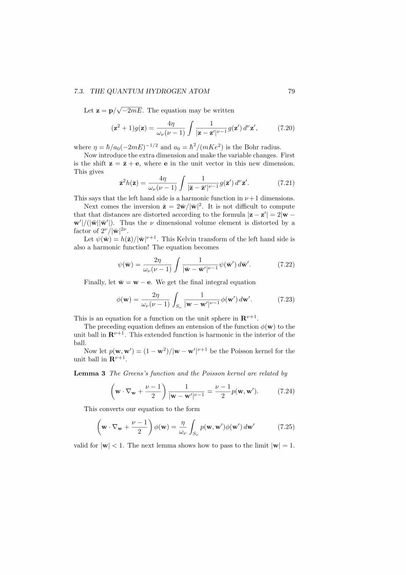
7.3. THE QUANTUM HYDROGEN ATOM 79
Let z = p/√−2mE. The equation may be written
(z2 + 1)g(z) =4η
ων(ν − 1)
∫1
|z− z′|ν−1g(z′) dνz′, (7.20)
where η = h/a0(−2mE)−1/2 and a0 = h2/(mKe2) is the Bohr radius.Now introduce the extra dimension and make the variable changes. First
is the shift z = z + e, where e in the unit vector in this new dimension.This gives
z2h(z) =4η
ων(ν − 1)
∫1
|z− z′|ν−1g(z′) dν z′. (7.21)
This says that the left hand side is a harmonic function in ν+1 dimensions.Next comes the inversion z = 2w/|w|2. It is not difficult to compute
that that distances are distorted according to the formula |z− z′| = 2|w−w′|/(|w||w′|). Thus the ν dimensional volume element is distorted by afactor of 2ν/|w|2ν .
Let ψ(w) = h(z)/|w|ν+1. This Kelvin transform of the left hand side isalso a harmonic function! The equation becomes
ψ(w) =2η
ων(ν − 1)
∫1
|w − w′|ν−1ψ(w′) dw′. (7.22)
Finally, let w = w − e. We get the final integral equation
φ(w) =2η
ων(ν − 1)
∫Sν
1
|w −w′|ν−1φ(w′) dw′. (7.23)
This is an equation for a function on the unit sphere in Rν+1.The preceding equation defines an entension of the function φ(w) to the
unit ball in Rν+1. This extended function is harmonic in the interior of theball.
Now let p(w,w′) = (1−w2)/|w−w′|ν+1 be the Poisson kernel for theunit ball in Rν+1.
Lemma 3 The Greens’s function and the Poisson kernel are related by(w · ∇w +
ν − 1
2
)1
|w −w′|ν−1=ν − 1
2p(w,w′). (7.24)
This converts our equation to the form(w · ∇w +
ν − 1
2
)φ(w) =
η
ων
∫Sν
p(w,w′)φ(w′) dw′ (7.25)
valid for |w| < 1. The next lemma shows how to pass to the limit |w| = 1.
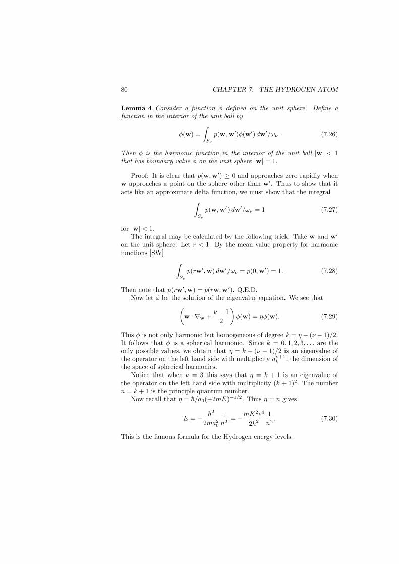
80 CHAPTER 7. THE HYDROGEN ATOM
Lemma 4 Consider a function φ defined on the unit sphere. Define afunction in the interior of the unit ball by
φ(w) =
∫Sν
p(w,w′)φ(w′) dw′/ων . (7.26)
Then φ is the harmonic function in the interior of the unit ball |w| < 1that has boundary value φ on the unit sphere |w| = 1.
Proof: It is clear that p(w,w′) ≥ 0 and approaches zero rapidly whenw approaches a point on the sphere other than w′. Thus to show that itacts like an approximate delta function, we must show that the integral∫
Sν
p(w,w′) dw′/ων = 1 (7.27)
for |w| < 1.The integral may be calculated by the following trick. Take w and w′
on the unit sphere. Let r < 1. By the mean value property for harmonicfunctions [SW] ∫
Sν
p(rw′,w) dw′/ων = p(0,w′) = 1. (7.28)
Then note that p(rw′,w) = p(rw,w′). Q.E.D.Now let φ be the solution of the eigenvalue equation. We see that(
w · ∇w +ν − 1
2
)φ(w) = ηφ(w). (7.29)
This φ is not only harmonic but homogeneous of degree k = η− (ν − 1)/2.It follows that φ is a spherical harmonic. Since k = 0, 1, 2, 3, . . . are theonly possible values, we obtain that η = k + (ν − 1)/2 is an eigenvalue ofthe operator on the left hand side with multiplicity aν+1
k , the dimension ofthe space of spherical harmonics.
Notice that when ν = 3 this says that η = k + 1 is an eigenvalue ofthe operator on the left hand side with multiplicity (k + 1)2. The numbern = k + 1 is the principle quantum number.
Now recall that η = h/a0(−2mE)−1/2. Thus η = n gives
E = − h2
2ma20
1
n2= −mK
2e4
2h2
1
n2. (7.30)
This is the famous formula for the Hydrogen energy levels.

7.4. THE HYDROGEN DEGENERACY 81
The treatment of the quantum mechanical Hydrogen atom with higherdimensional symmetry goes back to V. Fock in 1935. Much more is knownabout the symmetry of the hydrogen atom; the positive part of the spec-trum may also be treated this way [1]. (There is also an interesting directconnection with the quantum harmonic oscillator [3].)
Problems
1. Let E be the Euler operator and ∆ be the Laplace operator. Showthat ∆E − E∆ = 2∆.
2. Show that if g is harmonic, then Eg is harmonic.
7.4 The Hydrogen degeneracy
Now we fix the physical dimension ν = 3. For a spherical symmetric prob-lem in three dimensions one expects a multiplicity or degeneracy of eigen-values of a3
` = 2` + 1. This ` is the azimuthal quantum number. Recall
that a3` =
∑`m=0 a
2m where m is the magnetic quantum number.
Due to spherical symmetry in four dimensions get a4k = (k + 1)2 = n2
degeneracy, where n = k+ 1 is the principal quantum number. Recall thata4k =
∑k`=0 a
3` =
∑k`=0(2`+ 1) where ` is the azimuthal quantum number.
We have seen that the eigenvalue is −R 1(k+1)2 = −R 1
n2 where R =
mK2e4/(2h2).The actual situation is complicated by the fact that the electron has
spin. For our present purposes this simply means that the Hilbert spacecomes in two identical copies, so that all eigenvalues have a multiplicitytwo due to spin. Thus in the presence of spin a general spherically sym-metric problem will have eigenvalues with degeneracies 2(2`+ 1), while theHydrogen atom problem with its extra symmetry will have degeneracies2n2.
Here is a table of (n, `) states for the Hydrogen atom. Each entry in acolumn with angular momentum ` corresponds to 2(2` + 1) states. Thusthe numbers corresponding to an entry in the first four columns are 2, 6,10, 14. Each row corresponds to a state of degeneracy 2n2. Thus the sumfor the first four rows are 2, 8, 18, and 32. This is displayed in Table 1.
7.5 The periodic table
The Hydrogen atom problem is the beginning of an understanding of theentire periodic table of the elements. The elements are numbered by a
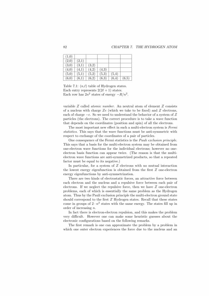
82 CHAPTER 7. THE HYDROGEN ATOM
(1,0)(2,0) (2,1)(3,0) (3,1) (3,2)(4,0) (4,1) (4,2) (4,3)(5,0) (5,1) (5,2) (5,3) (5,4)(6,0) (6,1) (6,2) (6,3) (6,4) (6,5)
Table 7.1: (n,`) table of Hydrogen states.Each entry represents 2(2`+ 1) states.Each row has 2n2 states of energy −R/n2.
variable Z called atomic number. An neutral atom of element Z consistsof a nucleus with charge Ze (which we take to be fixed) and Z electrons,each of charge −e. So we need to understand the behavior of a system of Zparticles (the electrons). The correct procedure is to take a wave functionthat depends on the coordinates (position and spin) of all the electrons.
The most important new effect in such a multi-electron system is Fermistatistics. This says that the wave functions must be anti-symmetric withrespect to exchange of the coordinates of a pair of particles.
One consequence of the Fermi statistics is the Pauli exclusion principle.This says that a basis for the multi-electron system may be obtained fromone-electron wave functions for the individual electrons; however no one-electron basis function can appear twice. (The reason is that the multi-electron wave functions are anti-symmetrized products, so that a repeatedfactor must be equal to its negative.)
In particular, for a system of Z electrons with no mutual interactionthe lowest energy eigenfunction is obtained from the first Z one-electronenergy eigenfunctions by anti-symmetrization.
There are two kinds of electrostatic forces, an attractive force betweeneach electron and the nucleus and a repulsive force between each pair ofelectrons. If we neglect the repulsive force, then we have Z one-electronproblems, each of which is essentially the same problem as the Hydrogenatom. Thus by the Pauli exclusion principle the multi-electron ground stateshould correspond to the first Z Hydrogen states. Recall that these statescome in groups of 2 · n2 states with the same energy. The states fill up inorder of increasing n.
In fact there is electron-electron repulsion, and this makes the problemvery difficult. However one can make some heuristic guesses about theelectronic configurations based on the following remarks.
The first remark is one can approximate the problem by a problem inwhich one outer electron experiences the force due to the nucleus and an

7.5. THE PERIODIC TABLE 83
average force due the the other electrons. The nucleus has charge Ze andthe other Z−1 electrons have total charge −(Z−1)e, so the outer electronshould find itself in orbit about a spread-out positive charge of e. So in thisapproximation the situation is very much like the Hydrogen problem. Thestate of lowest n compatible with the exclusion principle should determinethe ground state of the atom.
There is however, an important difference. For the Hydrogen problemthe energy level depends only on the principal quantum number n. Forthe present problem it also depends on the angular momentum quantumnumber `. The reason is that when ` is small, the wave function has asignificant part that is concentrated near the nucleus, inside the orbits of theother electrons. Thus the effect of the nuclear charge Ze is not completelycompensated by the the charge −(Z − 1)e of the other electrons. Theoutermost electron with small ` experiences a stronger attractive force andhas a lower energy. Thus the lowest energy state of the atom should comewhen the n and ` for the outer electron are both small.
What combination of n and ` should be minimized? The empirical factsare fairly well summarized in the n+` rule. (Recall that 0 ≤ ` ≤ n−1.) Thisrule says that to find the next one-electron state that is filled in buildingup the ground state of the multi-electron atom, first minimize n+ `. Thenminimize n.
This rule allows a prediction of the properties of the outer electronsin the periodic table. In the first version the table is listed by increasingZ. Each entry is characterized by listing the values of n and of `. The Zthat have a given value of n and ` are grouped in one entry. The numberof elements that correspond to an entry in one of the columns is given by2(2`+ 1), that is, by 14, 10, 6, 2 for angular momentum 3,2,1,0. These arelisted in Table 2. Notice that in this arrangement each row has decreasing
(1,0)(2,0)
(2,1) (3,0)(3,1) (4,0)
(3,2) (4,1) (5,0)(4,2) (5,1) (6,0)
(4,3) (5,2) (6,1) (7,0)
Table 7.2: (n,`) table of elements from n+ ` rule.Each entry represents 2(2`+ 1) elements.
` values.In the conventional periodic table the final ` = 0 values are grouped

84 CHAPTER 7. THE HYDROGEN ATOM
with the following decreasing sequence of values of ` ≥ 1. Thus the numberof elements that goes with an entry in one of the columns is 2, 14,10, 6.The totals that go with the first six rows are thus 2, 8, 8, 18, 18, 32. Thisis shown in Table 3.
(1,0)(2,0) (2,1)(3,0) (3,1)(4,0) (3,2) (4,1)(5,0) (4,2) (5,1)(6,0) (4,3) (5,2) (6,1)(7,0) (5,3)
Table 7.3: (n, `) values in periodic table of elements.Each entry represents 2(2`+ 1) elements.Arrangement is ` = 0, 3, 2, 1.
If we put in the atomic numbers in this order we get something veryclose to the periodic table from chemistry. The first two columns are the2 ` = 0 states. The next column replaces the 14 columns correspondingto ` = 3. The next 10 columns are the ` = 2 states. The final 6 columnsare the ` = 1 states. One should compare this ideal table with the actualperiodic table; they are almost the the same. With careful inspection onecan see the patterns of three and even four dimensional spherical harmonicsin the properties of the chemical elements. The full glory is seen in Table 4.
1 23 4 5 6 7 8 9 1011 12 13 14 15 16 17 1819 20 21 22 23 24 25 26 27 28 29 30 31 32 33 34 35 3637 38 39 40 41 42 43 44 45 46 47 48 49 50 51 52 53 5455 56 57–70 71 72 73 74 75 76 77 78 79 80 81 82 83 84 85 8687 88 89–102
Table 7.4: Z values in ideal periodic table of elements.Arrangement is ` = 0, 3, 2, 1.
There is another terminology for the angular momentum values ` =0, 1, 2, 3 that came from spectrographic history and is now standard inchemistry. The numbers are replaced by the letters s, p, d, f. (The firstthree letters are not in any particular sequence, but come from empirical
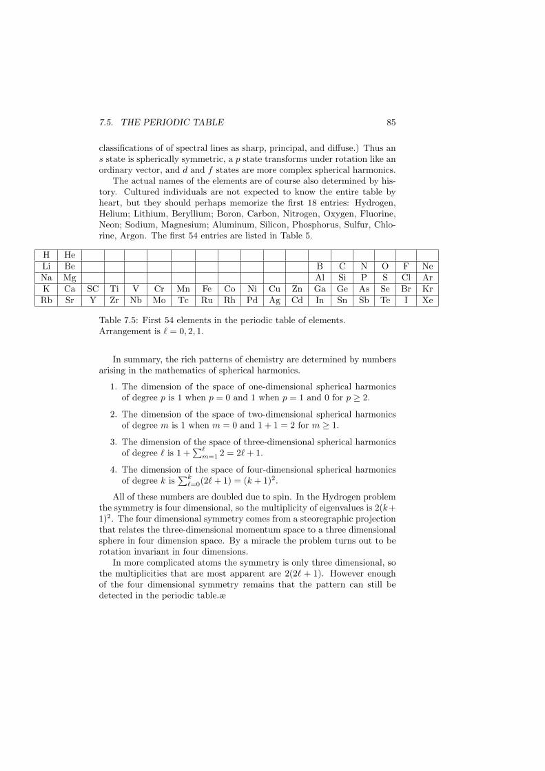
7.5. THE PERIODIC TABLE 85
classifications of of spectral lines as sharp, principal, and diffuse.) Thus ans state is spherically symmetric, a p state transforms under rotation like anordinary vector, and d and f states are more complex spherical harmonics.
The actual names of the elements are of course also determined by his-tory. Cultured individuals are not expected to know the entire table byheart, but they should perhaps memorize the first 18 entries: Hydrogen,Helium; Lithium, Beryllium; Boron, Carbon, Nitrogen, Oxygen, Fluorine,Neon; Sodium, Magnesium; Aluminum, Silicon, Phosphorus, Sulfur, Chlo-rine, Argon. The first 54 entries are listed in Table 5.
H HeLi Be B C N O F NeNa Mg Al Si P S Cl ArK Ca SC Ti V Cr Mn Fe Co Ni Cu Zn Ga Ge As Se Br KrRb Sr Y Zr Nb Mo Tc Ru Rh Pd Ag Cd In Sn Sb Te I Xe
Table 7.5: First 54 elements in the periodic table of elements.Arrangement is ` = 0, 2, 1.
In summary, the rich patterns of chemistry are determined by numbersarising in the mathematics of spherical harmonics.
1. The dimension of the space of one-dimensional spherical harmonicsof degree p is 1 when p = 0 and 1 when p = 1 and 0 for p ≥ 2.
2. The dimension of the space of two-dimensional spherical harmonicsof degree m is 1 when m = 0 and 1 + 1 = 2 for m ≥ 1.
3. The dimension of the space of three-dimensional spherical harmonicsof degree ` is 1 +
∑`m=1 2 = 2`+ 1.
4. The dimension of the space of four-dimensional spherical harmonicsof degree k is
∑k`=0(2`+ 1) = (k + 1)2.
All of these numbers are doubled due to spin. In the Hydrogen problemthe symmetry is four dimensional, so the multiplicity of eigenvalues is 2(k+1)2. The four dimensional symmetry comes from a steoregraphic projectionthat relates the three-dimensional momentum space to a three dimensionalsphere in four dimension space. By a miracle the problem turns out to berotation invariant in four dimensions.
In more complicated atoms the symmetry is only three dimensional, sothe multiplicities that are most apparent are 2(2` + 1). However enoughof the four dimensional symmetry remains that the pattern can still bedetected in the periodic table.æ

86 CHAPTER 7. THE HYDROGEN ATOM

Part II
Self-adjoint Operators
87


Chapter 8
The spectral theorem
This chapter is devoted to the spectral theorem. We first prove the theoremfor unitary operators and then deduce the theorem for self-adjoint operatorsas a consequence. The first result is that a unitary operator is isomorphicto a multiplication operator acting in L2, where the multiplication is by afunction of absolute value one. The second result says that a self-adjointoperator is isomorphic to multiplication by a real function. The passagefrom the first to the second result is obtained by observing that a self-adjointoperator may always be expressed as a function of a unitary operator.
There are many proofs of the spectral theorem. All of them requiresome sort of approximation argument. However there are many variantsto the argument and many stages at which the argument can be applied.One can work directly with the self-adjoint operator [K, 9], one can workwith the resolvent [N2], one can work with the unitary Cayley transform[vN] (as we do), or one can work with the unitary group. There is a veryinteresting approach using the resolvent and contour integration [L].
8.1 Difference approximations
Our main interest is the spectral theorem for self-adjoint operators. How-ever we begin with some remarks meant to motivate the approach in termsof unitary operators.
The first thing to notice is that when a self-adjoint operator A has aspectral representation, then the Schrodinger equation has a nice solutionin terms of unitary operators. However even if there is a spectral represen-tation, one may not know very explicitly what it is. Therefore it would bedesirable to get at a solution without using the spectral representation.
89

90 CHAPTER 8. THE SPECTRAL THEOREM
One such strategy for solving the Schrodinger equation is by the use ofdifference methods. We shall assume that there is a spectral representationand explore the convergence of the difference methods.
Let ψ(t) = Utψ be the solution of the abstract Schrodinger equation
idψ(t)
dt= Aψ(t). (8.1)
Assume that we want to solve the equation by a finite difference method.One can approximate the equation by the forward difference approximation
i(ψ(t+ h)− ψ(t)) = hAψ(t). (8.2)
This has solutionψ(t+ h) = (1− ihA)ψ(t). (8.3)
The obvious attempt to find a solution of the differential equation is
Utψ = limn→∞
((1− i(t/n)A))nψ. (8.4)
However the conditions for convergence are going to be very delicate whenA is unbounded. Even though Ut is unitary, the approximating operatorsare not even continuous. This method is thus delicate theoretically anduseless in practice.
One can do much better with the backward difference approximation
i(ψ(t+ h)− ψ(t)) = hAψ(t+ h). (8.5)
This has solutionψ(t+ h) = (1 + ihA)−1ψ(t). (8.6)
which is expressed in terms of a bounded operator It is not difficult to verifythat the solution of the differential equation is
Utψ = limn→∞
((1 + i(t/n)A)−1
)nψ. (8.7)
However it is irritating that one is trying to approximate a unitary operatorby operators that are not unitary.
Perhaps best of all is the forward-backward difference approximation
i(ψ(t+ h)− ψ(t)) = hA(ψ(t+ h) + ψ(t))/2. (8.8)
This has solution
ψ(t+ h) = (1− (i/2)hA)(1 + (i/2)hA)−1ψ(t). (8.9)
8.2. SPECTRAL THEOREM FOR UNITARY OPERATORS 91
which is continuous. We have
Utψ = limn→∞
((1− (i/2)(t/n)A)(1 + (i/2)(t/n)A)−1
)nψ. (8.10)
This time the approximating operators are unitary.We thus see that there are several operators that are related to the
abstract Schrodinger equation. There is the operator A that defines theequation. There is the unitary group Ut = exp(−itA) that gives the solu-tion. The unitary group may be approximated by the backward differencemethod. This uses bounded operators of the form (1 − ihA)−1, where his real. Such an operator are called a resolvent operator of A. Finally theunitary group may be approximated by the forward-backward differencemethod. This uses unitary operators of the form U = (1 − i(h/2)A)(1 +i(h/2)A)−1, where h is real. Such an operator is called a Cayley transformof A.
The strategy for proving the spectral theorem is now clear. Start witha self-adjoint operator A. Consider its Cayley transform U . The integerpowers Un define an unitary dynamics that approximate the dynamics ofthe Schrodinger equation. Work with this dynamics to prove a spectraltheorem for the unitary operator. Then recover the spectral theorem forthe self-adjoint operator by the inverse of the Cayley transform.
One could also attempt to use the true Schrodinger dynamics to provethe spectral theorem. The trouble with this is that one then has to solvethe Schrodinger equation without use of a spectral representation. Thiscan be done by showing directly that the approximate dynamics convergeto the true dynamics, but this approach is slightly more technical.
8.2 Spectral theorem for unitary operators
We now investigate the structure of unitary operators from a Hilbert spaceto itself. This is the sort of operator we expect to encounter in quantummechanical time evolution. The fundamental result is the spectral theorem.
The strategy may be understood by looking at the case when there is abasis of eigenvectors, so that the unitary operator U satisfies Uφj = eiθjφj .Let ψ =
∑j cjφj be an arbitrary vector. Then
〈ψ,Unψ〉 =∑j
exp(inθj)|cj |2 =
∫ 2π
0
einθ dµ(θ), (8.11)
where dµ(θ) =∑j |cj |2δ(θ − θj) dθ. In this case the measure associated
with the operator U and the vector ψ is concentrated on those eigenvaluessuch that ψ has a non-zero component in the eigenvector direction.
92 CHAPTER 8. THE SPECTRAL THEOREM
Not every unitary operator has a basis of eigenvectors in the Hilbertspace. Correspondingly, not every spectral measure µ is discrete. Howeverthe above example suggests that one attempt to get at the measure µ byexpressing its integral with trigonometric functions einθ directly in termsof Hilbert space quantities. The following proposition shows that this canbe accomplished in general. The proof of the proposition will follow fromthe two lemmas immediately below.
Proposition 25 Let U be a unitary operator from H to itself. Let ψ be a(unit) vector in H. Then there exists a (probability) measure µ on the unitcircle such that
〈ψ,Unψ〉 =
∫ 2π
0
einθ dµ(θ). (8.12)
In order to prove this result we must first characterize the functionsof the form un = 〈ψ,Unψ〉. Let u be a function from the integers to thecomplex numbers. Then u is said to be of positive type if for every sequencea of complex numbers with finite support∑
m
∑n
a∗mun−man ≥ 0. (8.13)
Notice that if u is of positive type, then in particular for each n the 2by 2 matrix (
u0 unu−n u0
)(8.14)
is positive. As a consequence u0 ≥ 0, u−n = u∗n, and |un| ≤ u0.
Lemma 5 Let U be a unitary operator and ψ be a vector in H. Thenun = 〈ψ,Unψ〉 is a positive type function of the integer variable n.
Proof: Let U be a unitary operator and ψ be a vector in H. ThenU∗ = U−1 and so
〈Umψ,Unψ〉 = 〈ψ,Um∗Unψ〉 = 〈ψ,Un−mψ〉. (8.15)
Then
0 ≤ ‖∑n
anUnψ‖2 = 〈
∑m
amUmψ,
∑n
anUnψ〉 =
∑m
∑n
a∗m〈ψ,Un−mψ〉an.
(8.16)
Lemma 6 Let u be a function of positive type. Then there exists a uniquemeasure µ on the unit circle such that
un =
∫ 2π
0
einθ dµ(θ). (8.17)
8.2. SPECTRAL THEOREM FOR UNITARY OPERATORS 93
Proof: A trigonometric polynomial is a function of the form p(eiθ) =∑cne
inθ, a polynomial in positive and negative powers of eiθ. It is afunction on the unit circle. We associate to each such polynomial thecomplex number L(p) =
∑cnun. This is clearly linear.
If the polynomial is real, then c−n = c∗n. Since also u−n = u∗n, it followsthat L(p) is real.
A lemma of Fejer and Riesz (see below) says that if a trigonometricpolynomial satisfies p(eiθ) ≥ 0, then there exists another trigonometricpolynomial q(eiθ) such that p(eiθ) = |q(eiθ)|2. Set q(eiθ) =
∑n ane
inθ.It then follows from the positive type condition that L(p) = L(|q|2) =∑m
∑n a∗manun−m ≥ 0.
To each trigonometric polynomial p(eiθ) we have associated the numberL(p). This assigns positive numbers to positive polynomials. It followsthat the operation preserves order. It also send constant polynomials tothe corresponding constant times u0. In particular, if −c ≤ p(eiθ) ≤ c, then−cu0 ≤ L(p) ≤ cu0. In other words this is a continuous linear functional ontrigonometric polynomials, with the norm of uniform convergence. It is wellknown (for example from the Stone-Weierstrass approximation theorem)that trigonometric polynomials on the circle are dense in the continuousfunctions on the circle. It follows that this is a continuous linear functionalon the continuous functions. It is a well-known theorem of Riesz that everysuch functional determines a measure (that is, an integral in the sense we
have discussed). So we have L(p) =∫ 2π
0p(eiθ) dµ(θ), where the integration
is over the circle. Q.E.D.
Remark: The claim is that the integral satisfies all the properties ofthe integral, including the monotone convergence theorem. In particular,the original functional L defined on the continuous functions must satisfythe monotone convergence theorem. It is natural to ask why this shouldalways be so. This is explained by Dini’s theorem, a result about con-tinuous functions on a compact space. The theorem says that monotonepointwise convergence of continuous functions to a continuous function im-plies uniform convergence. Of course this in turn implies convergence ofthe functionals.
In the above proof we used the lemma of Fejer and Riesz.
Lemma 7 If the trigonometric polynomial p(eiθ) is positive, then there ex-ists another trigonometric polynomial polynomial q(eiθ) such that p(eiθ) =|q(eiθ)|2.
Proof: This is a result about trigonometric polynomials, which maybe thought of as ordinary polynomials in z and z−1, where the complexnumber z is restricted to the unit circle |z| = 1. We may as well assume
94 CHAPTER 8. THE SPECTRAL THEOREM
in the proof that p(z) > 0 for |z| = 1, since the hypothesis as stated is alimiting case.
We now look at these polynomials without the restriction that |z| = 1.The reality condition translates to the condition p(z) = p(1/z∗)∗. Nowassume that p(z) is of degree k in z and 1/z. Then r(z) = zkp(z) is ofdegree 2k in z. Furthermore r(z) = z2kr(1/z∗)∗. From this it is clear thatfor every root a of r(z), there is a corresponding root 1/a∗. Since p(z) hasno roots on the unit circle, neither does r(z). Hence the roots of r(z) occurin pairs. This gives the representation
r(z) = b∏i
(z − ai)(z − 1/a∗i ). (8.18)
This converts into a representation
p(z) = c∏i
(z − ai)(1/z − a∗i ). (8.19)
In order to have p(z) > 0 for |z| = 1 we must have c > 0. Therefore we maytake q(z) =
√c∏i(z− ai). When we restrict to the unit circle, we may use
1/z = z∗, and so p(z) = q(z)q(z)∗ = |q(z)|2. Q.E.D.
Theorem 19 Let U be a unitary operator from H to itself. Then thereexists a measure space and associated Hilbert space L2(X,µ) of square-integrable functions, an isomorphism W from H to L2, and a measurablefunction υ with |υ| = 1 such that U = W−1υW . Every unitary operator isisomorphic to a multiplication operator (multiplication by a function withmodulus one).
Proof: For a unit vector ψ in H let Hψ be the closed linear subspacegenerated by Unψ for integer n. Then U restricted to Hψ is a unitaryoperator. The first part of the proof is to prove a spectral representationfor this restricted operator.
Since U is unitary, for every trigonometric polynomial q(eiθ) with p(eiθ) =q(eiθ)∗q(eiθ) we have p(U) = q(U)∗q(U). Therefore for every trigonometricpolynomial q(eiθ) we have
‖q(U)ψ‖2 = 〈ψ, q(U)∗q(U)ψ〉 =
∫ 2π
0
q(eiθ)∗q(eiθ) dµ(θ) =
∫ 2π
0
|q(eiθ)|2 dµ(θ).
(8.20)Therefore if q(U)ψ = 0, then q(eiθ) = 0 for all θ except for a set of µmeasure zero. Therefore q(eiθ) is a nul function and may be identified withzero in the space L2(S, µ) of square-integrable functions on the circle.
8.2. SPECTRAL THEOREM FOR UNITARY OPERATORS 95
It follows that we may define an unitary operator Wψ from Hψ to L2(S, dµ) by Wψq(U)ψ = q(eiθ). (Note that in particular Wψψ = 1.)Furthermore it is easy to check that WψUq(U)ψ = eiθWψq(U)ψ. It followsby continuity that WψUχ = eiθWψχ for all χ in Hψ. That is, we have aspectral representation for the part of U in the subspace Hψ.
The second part of the proof is to piece together these spectral repre-sentations for subspaces into a spectral representation for the entire space.Consider families ψj of vectors such that Hψj are mutually orthogonal.Take a maximal such family.
Let M be the closed linear subspace of consisting of all vectors φ =∑j φj where φj is in Hψj .
Lemma 8 Let U be a unitary operator from H to itself. Let M be a closedlinear subspace of H that is invariant under U and U−1. Then M⊥ isinvariant under U and U−1.
By use of the lemma we see that M = H. If this were not the case,then by the projection theorem there would be a unit vector ψ orthogonalto M . Then we could construct another closed linear subspace Hψ. Thiswould contradict the maximality.
Now take as many copies Sj of the unit circle as there are vectors ψj .Let X be the disjoint union of the Sj . Each point x in X is determined bya pair (θ, j). For each j the measure µj is the measure determined by Uand ψj . Define the measure µ to be the measure that restricts to µj on thejth circle. Define the function υ by υ(x) = υ(θ, j) = eiθ.
Now for every φ in H we define
Wφ(x) = Wφ(θ, j) = Wψjφj(θ). (8.21)
It is easy to check that for each x = (θ, j) in X we have
WUφ(x) = WψjUφj(θ) = eiθWψjφj(θ) = υ(x)Wφ(x). (8.22)
Thus we have found the required spectral representation. Q.E.D.The construction in the proof of the theorem gives a measure, but does
not tell much about whether the measure is point or continuous. It isimportant to note that in either case certain functions that are are verydifferent may define the same member of L2. In particular, when the mea-sure consists only of masses at certain points, then the values of functionsmatter only at these points. In this case one is essentially dealing with aspace `2, even though the construction might not immediately suggest it.
Our construction gave the space X as a disjoint union of circles, butthe nature of the L2 spaces obtained depend very much on the measures

96 CHAPTER 8. THE SPECTRAL THEOREM
on these circles. It is essential to realize that the actual nature of the spaceX depends on the particular proof method and is largely irrelevant. Onthe other hand, the fact that the range of the multiplication operator iscontained in the unit circle is essential for it to be unitary.
Problems
1. Let U be a unitary operator such that U has a basis of eigenvectors.Take the ψj in the proof of the spectral theorem to be the correspond-ing eigenvectors. Describe the measure µ and function υ given by theproof of the spectral theorem.
2. Let U be a unitary operator such that U has a countable basis ofeigenvectors φj . Assume that each eigenvalue has multiplicity one.Take the ψ in the proof of the spectral theorem to be ψ =
∑j cjφj
where all the coefficients are non-zero. Describe the measure µ andfunction υ given by the proof of the spectral theorem.
3. Let the Hilbert space be L2(S, dθ), where S is the unit circle, and letUa be rotation by the angle a. In order to stay within the frameworkof the previous problem, take a to be an irrational multiple of 2π.Let ψ be a function whose Fourier coefficients never vanish. Find themeasure µ and function υ given by the proof of the spectral theorem.
4. Let the Hilbert space be L2(R, dx) and let Ua be translation by a.Let ψ be a function whose Fourier transform never vanishes. Find themeasure µ and function υ given by the proof of the spectral theorem.
8.3 Graphs
In this section we use the Pauli matrices to manipulate linear graphs. Thefirst Pauli matrix is just an interchange.
σ1 =
(0 11 0
)(8.23)
The second one involves a change of sign and an interchange. There isalso a conventional factor of i, which serves to make its square equal toone. (This factor will play no role in our considerations, since we will beapplying the matrix only to subspaces.)
σ2 = i
(0 −11 0
)(8.24)

8.3. GRAPHS 97
The third one involves only a change of sign.
σ3 =
(1 00 −1
)(8.25)
Consider the direct sum Hilbert spaceH⊕H. This consists of all orderedpairs (ψ, φ) with the obvious vector space operations. The inner product is
〈(ψ, φ), (ψ′, φ′)〉 = 〈ψ,ψ′〉+ 〈φ, φ′〉. (8.26)
The Pauli matrices act on the direct sum Hilbert space in a natural way.They each define a unitary operator whose square is one.
Definition 13 A graph is a linear subspace of H⊕H.
If A is a graph, then we may apply the Pauli matrices to the pairs inthe graph to get a new graph. Thus we define the inverse A−1 as σ1A. Thenegative inverse −A−1 is σ2A. Finally the negative −A is σ3A.
Notice that taking the closure of a graph commutes with each of thesethree operations, for instance A−1 = (A−1) .
If A is a graph, then its domain D(A) consists of all ψ in H such thatthere exists a φ in H with (ψ, φ) in A. Its range R(A) consists of all φ inH such that there exists a ψ in H with (ψ, φ) in A.
If A is a graph, then its nullspace N(A) consists of all ψ in H suchthat (ψ, 0) is in A. This is obviously a subset of the domain D(A). Thecorresponding subset of R(A) = D(A−1) is N(A−1).
It is worth noting that if A is closed as a subspace of H⊕H, then N(A)and N(A−1) are also closed as subspaces of H.
Definition 14 An operator is a graph such that the only pair of the form(0, φ) in the graph is (0, 0). When a pair (ψ, φ) is in a graph A that is anoperator, then we write Aψ = φ.
Notice that A is an operator if and only if N(A−1) consists only of thezero vector.
Problems
1. Show that an operator has a closed graph if and only if its domainwith the graph norm is a Hilbert space.
2. Must the closure of the graph of an operator be the graph of anoperator?
98 CHAPTER 8. THE SPECTRAL THEOREM
8.4 Adjoints
Definition 15 The adjoint graph A∗ is defined to be (σ2A)⊥ = σ2A⊥.
Notice that it does not matter whether we take the orthogonal complementbefore or after applying the unitary operator.
It is easy to check that (σ1A)⊥ is −A∗ = (−A)∗. Also (σ3A)⊥ is A∗−1 =A−1∗.
Theorem 20 The closure of the graph and the adjoint are related by A∗ =A∗ and A = A∗∗.
Proof: Since A⊥ = A⊥, we have A∗ = A∗. Similarly, from the projectiontheorem we have A = A⊥⊥. This gives A = A∗∗. Q.E.D.
One main reason for the introduction of the adjoint concept is that itgives information about ranges, that is about finding solutions of equations.
Proposition 26 We have the relations N(A∗) = R(A)⊥ and N(A) =R(A)∗⊥.
There is a dual result for domains.
Proposition 27 We have the relations N(A∗−1) = D(A)⊥ and N(A−1) =D(A∗)⊥.
Notice that A is an operator if and only if N(A−1) consists only ofthe zero vector. Therefore A∗ is an operator if and only if D(A) is dense.Similarly A is an operator if and only if D(A∗) is dense.
From this it is easy to see that the class of densely defined closed oper-ators is a particularly nice class. If A is densely defined and closed, then sois A∗, and A∗∗ = A.
The most important classes of graphs are skew-adjoint, self-adjoint, andunitary. It is amusing that these correspond exactly to the Pauli matricesσ1, σ2, and σ3.
Definition 16 We define a graph A to be skew-adjoint if (σ1A)⊥ = −A∗ =A.
Definition 17 We define a graph A to be self-adjoint if (σ2A)⊥ = A∗ = A.
Definition 18 We define a graph U to be unitary if (σ3A)⊥ = A−1∗ = A.
Proposition 28 A unitary graph is an operator.

8.5. SPECTRAL THEOREM FOR SELF-ADJOINT OPERATORS 99
Proof: Let U be a unitary graph. Assume that (0, φ) is in U . Then(0, φ) is orthogonal to σ3(0, φ) = (0,−φ), so φ is orthogonal to φ, and φmust be zero. Q.E.D.
It is not difficult to check that a unitary operator as defined here is thesame notion as before: an isomorphism of the Hilbert space onto itself.
Problems
1. Show that a self-adjoint graph that is an operator is the same as aself-adjoint operator as previously defined.
8.5 Spectral theorem for self-adjoint opera-tors
The Pauli matrices are two-by-two unitary matrices with eigenvalues ±1.Therefore they are all unitarily equivalent. Thus, for instance, we may finda unitary operator τ such that
τσ2 = σ3τ. (8.27)
Let A be a self-adjoint graph, and define U = τA. It follows that
U = τA = τA∗ = τσ2A⊥ = σ3τA
⊥ = σ3U⊥ = U∗−1. (8.28)
Let us look more explicitly at the form of this relation. Take for instance
τ =1√2
(1 i1 −i
)(8.29)
Then if (ψ, φ) is in the graph of A, the corresponding element of the graphof U is a multiple of (ψ+ iφ, ψ− iφ). In other words, U(ψ+ iφ) = (ψ− iφ).
We may solve this equation by (1− U)ψ = i(1 + U)φ. We see that theself-adjoint graph A is an operator if and only if U has no eigenvectors witheigenvalue −1.
The spectral theorem for unitary operators now immediately gives thespectral theorem for self-adjoint operators.
Theorem 21 Let A be a self-adjoint operator from H to itself. Then thereexists a measure space L2(X,µ) and an isomorphism W from H to L2 anda real measurable function α such that A = W−1αW . Every self-adjointoperator is isomorphic to a multiplication operator (multiplication by a realfunction).

100 CHAPTER 8. THE SPECTRAL THEOREM
Proof: Define the unitary operator U by
U(ψ + iAψ) = ψ − iAψ (8.30)
as above. Since A is an operator, −1 is not an eigenvalue of U . Then
Aψ = −i(1 + U)−1(1− U)ψ. (8.31)
By the spectral theorem for unitary operators, U is isomorphic to mul-tiplication by some υ with |υ| = 1. It follows that A is isomorphic tomultiplication by α given by α = −i(1 + υ)−1(1− υ). Q.E.D.
Notice that all this proof amounts to is to note that if A is a self-adjointoperator, then the Cayley transform U = (1 − i(h/2)A)(1 + i(h/2)A)−1 isunitary, and so the spectral theorem for unitary operators applies. As longas h 6= 0 one can solve for A in terms of U .
One immediate consequence is that the unitary group Ut = exp(−itA)giving the Schrodinger time evolution is defined. Furthermore, it is also easyto see (now that the spectral theorem is available) that the approximateunitary dynamics Un given by the Cayley transform converges strongly tothe exact dynamics Ut as n→∞ and h→ 0 with nh→ t.
Problems
1. Show that the Cayley transform U = (1 − iA)(1 + iA)−1 may beexpressed in terms of the resolvent as U = 2(1 + iA)−1 − 1.
2. Let A be a self-adjoint operator such that A has a basis of eigen-vectors. Take the ψj in the proof of the spectral theorem to be thecorresponding eigenvectors. Describe the measure µ and function αgiven by the proof of the spectral theorem.
3. Let A be a self-adjoint operator such that A has a countable basisof eigenvectors φj . Assume that each eigenvalue has multiplicity one.Take the ψ in the proof of the spectral theorem to be ψ =
∑j cjφj
where all the coefficients are non-zero. Describe the measure µ andfunction α given by the proof of the spectral theorem.
4. Let H = L2(R, dx) and A = −id/dx. Find the Cayley transform Uas an integral operator.
5. Let A be a self-adjoint operator. Define U = (1 − i(h/2)A)(1 +i(h/2)A)−1. Let Ut = exp(−itA). Show that for each ψ the vectorsUnψ converge to Utψ as n→∞ and h→ 0 with nh→ t.
6. State and prove a spectral theorem for self-adjoint graphs.
æ

Chapter 9
Functions of self-adjointoperators
This chapter is devoted to complex functions of a self-adjoint operator.The most important are the resolvent and the unitary group. By the spec-tral theorem, these are families of operators isomorphic to multiplicationoperators on L2.
One important application is to the energy operator H of quantummechanics. If this is a self-adjoint operator, then the corresponding unitarygroup exp(−itH/h) solves the Schrodinger equation.
The spectral theorem plays an important role in the interpretation ofquantum mechanics. For an arbitrary unit vector and self-adjoint operator,it gives a realization of the operator as a random variable on a probabilityspace determined by the operator and by the vector.
In the case of the energy operator, the realization as a random variableis independent of time. This random variable specifies for the solution howmuch probability is associated with each set of energies.
9.1 Functional calculus
The spectral theorem says that a self-adjoint operator has the representa-tion
A = W−1αW. (9.1)
(As usual we write α both for the function and the corresponding multi-plication operator.) Consider a complex Borel function f defined on theline (or at least on the range of α). It is natural to attempt to define an
101
102 CHAPTER 9. FUNCTIONS OF SELF-ADJOINT OPERATORS
arbitrary complex Borel function f(A) of a self-adjoint operator A by
f(A) = W−1f(α)W. (9.2)
This turns out to be a good definition. It is not immediately obvious thatit is independent of the spectral representation, but that is in fact the case[N2]. We shall see why this is so in the discussion below.
One of the most important functions is the resolvent (A − z)−1. Thisis certainly defined for all z that are not real, and in this case it is obviousthat this is a bounded operator with bound ‖(A − z)−1‖ ≤ 1/|=z|. Theresolvent is obviously well defined independent of the spectral resolution.
The complement of the set where the resolvent is defined as a boundedoperator is called the spectrum. The spectrum is always a closed set. Wehave seen that the spectrum of a self-adjoint operator A is real. It is clearfrom the spectral theorem that the spectrum is the essential range of therepresenting function α. Therefore in defining functions f(A) we only needto worry about f being defined on the spectrum. In particular, the resolvent(A− z)−1 is defined whenever z is not in the spectrum of A and it satisfiesthe bound ‖(A−z)−1‖ ≤ 1/d(z), where d(z) is the distance to the spectrum.Notice that d(z) ≤ |=z|, so this is a generalization of the bound given inthe preceding paragraph.
The Cayley transform that we have been considering is closely relatedto the resolvent; in fact for each real h 6= 0
U = (1− i(h/2)A)(1 + i(h/2)A)−1 = −1 + (4i/h)(A− 2i/h)−1. (9.3)
If f is a complex Borel function defined on the spectrum of A, thenf(A) = h(U), where h(u) = f((2i/h)(1− u)/(1 + u)). So in order to showthat f(A) is independent of the spectral representation, it is enough toshow that h(U) is independent of the spectral representation.
This is certainly true for polynomials in positive and negative powersof U . Now observe that if hn is a sequence of functions bounded by a fixedconstant for which hn(U) is uniquely defined, and hn → h pointwise, thenhn(U) → h(U) strongly, and so h(U) is uniquely defined. By repeatedlimiting operations we may obtain in this way all bounded complex Borelfunctions h on the circle.
This shows the uniqueness of the definition of f(A), at least for boundedfunctions f . However if f is not bounded, but f(A)ψ is defined, then thereis a sequence of bounded functions fn that converges to f pointwise andsuch that fn(A)ψ converges to f(A)ψ. This shows that even in this casef(A) is uniquely defined.
One useful class of functions of A consists of the functions that havevalues 0 or 1. Let 1S be the function that is 1 on the Borel set S (a
9.2. SOME USEFUL FUNCTIONS 103
subset of the real line) and 0 on its complement. Then 1S(A) is calledthe spectral projection of A corresponding to the set S. It is an orthogonalprojection onto a closed subspace of the Hilbert space. This subspace shouldbe thought of as the part of the Hilbert space where A has values in S.
Problems
1. What is the spectrum of 1S(A)? Consider all cases.
2. Consider the restriction of A to the range of 1S(A). Show that thespectrum of this restricted operator is contained in the closure of S.
3. Give an example where it is not contained in S.
9.2 Some useful functions
It is nice to be able to define arbitrary functions of a self-adjoint operator,but certain functions are particularly important. Perhaps the most impor-tant are the resolvent and the unitary group. From the resolvent one canconstruct approximate delta functions, and with these one can approximatea wide class of functions.
If A is a self-adjoint operator, then we may define the approximate deltafunction operator for ε > 0 by
δε(A− a) =1
π
ε
(A− a)2 + ε2=
1
2πi
((A− a− iε)−1 − (A− a+ iε)−1
).
(9.4)
The last equation is important because it says that the approximatedelta function is defined by the resolvent (A− z)−1 for z not real.
Proposition 29 If f is bounded and continuous, then f(A) is determinedby ∫
f(A)ψ = limε→0
∫f(a)δε(A− a)ψ da. (9.5)
Proof: If f is bounded and continuous, then∫f(a)δε(α(x)− a) da→ f(α(x)) (9.6)
as ε→ 0 pointwise. The result follows from the L2 dominated convergencetheorem.
104 CHAPTER 9. FUNCTIONS OF SELF-ADJOINT OPERATORS
Corollary 7 The unitary group is expressed in terms of the resolvent by∫exp(−itA)ψ = lim
ε→0
∫exp(−ita)δε(A− a)ψ da. (9.7)
It is also possible to go from the resolvent to the unitary group. Theresolvent is given by a time integral. The integral goes over positive time ornegative time depending on whether z is in the upper or lower half plane.
Proposition 30 The resolvent is given in terms of the unitary group by
(A− z)−1ψ =
∫ ±∞0
i exp(itz) exp(−itA)ψ dt (9.8)
for ±z > 0.
The delta function is given by the jump in the resolvent between thelower and upper half plane. Thus in order to get the delta function we needto integrate over all time.
Corollary 8
δε(A− a)ψ =
∫ ∞−∞
exp(iat) exp(−ε|t|) exp(−itA)ψdt
2π. (9.9)
Problems
1. Let f be a bounded piecewise continuous function with right and lefthand limits at the points of discontinuity. How must f be defined atthe points of discontinuity so the formula for f(A) in terms of theapproximate delta function remains valid?
2. Under what circumstances does the result of the previous problemgive a formula for spectral projections in terms of the approximatedelta function?
3. Show that the strong limit as ε → 0 of πεδε(A − a) is the projectiononto the eigenspace where A = a.
9.3 Random variables
Let A be a self-adjoint operator. Then by the spectral theorem there isan isomorphism W from H to L2(X,µ). Under this isomorphism A isisomorphic to multiplication by a real function α.
9.3. RANDOM VARIABLES 105
Let ψ be a unit vector in the Hilbert space H. Then Wψ is a functionon X such that ∫
|Wψ(x)|2 dµ(x) = 1. (9.10)
Thus |Wψ(x)|2 dµ(x) is a probability measure. A measurable function ona space with a probability measure is called a random variable. Thus α isa random variable.
Take f to be a bounded Borel measurable function. Then f(α) is abounded random variable. The expectation of this random variable is
〈ψ, f(A)ψ〉 =
∫f(α(x))|Wψ(x)|2 dµ(x). (9.11)
This last equation is a remarkable correspondence between Hilbert spaceand probability expressions.
These considerations show that a unit vector and an arbitrary self-adjoint operator gives rise to a random variable. Of course, two non-commuting random variables will not give rise to random variables definedon the same probability space.
In quantum mechanics some self-adjoint operators may give rise to ran-dom variables having physical significance. One example is the energy op-erator H. Since the time development of ψ is given by the energy operatoras exp(−itH/h)ψ, the probability measure does not depend on time. Thedistribution of H gives the amount of probability corresponding to each setof energy values, and this amount does not change with time.
We may write the expectation of a function of a random variable interms of a measure on the reals, the distribution of the random variable. Iff is bounded and measurable, then we obtain
〈ψ, f(A)ψ〉 =
∫f(a) dν(a). (9.12)
The measure ν is uniquely determined by the unit vector and the self-adjointoperator. It is supported on the spectrum of the operator. A special caseof the above formula is
〈ψ, 1S(A)ψ〉 = ν(S). (9.13)
This is interpreted as the probability that A is in S. It is clear that calcu-lating the distribution ν must be one of the fundamental goals of quantummechanics.
It is perhaps useful at this point to summarize the basic principles ofquantum mechanics. A state of a system is determined by a unit vector ψ
106 CHAPTER 9. FUNCTIONS OF SELF-ADJOINT OPERATORS
in the Hilbert space H. Two vectors determine the same state if they aremultiples of each other. (Thus what is important is not the vector, but theone dimensional subspace, or ray, determined by the vector. The collectionof all these subspaces is actually a projective space rather than a vectorspace.)
An observable is determined by a self-adjoint operator. The fundamen-tal equation is that the expectation of a real measurable function of theoperator is given (when the relevant integral converges absolutely) by
〈ψ, f(A)ψ〉. (9.14)
In particular, when f has values only zero or one, this is the probabilitythat A has value in the set where f is one.
We may summarize this as follows.
Dogma 1 States are determined by unit vectors in Hilbert space. Observ-ables are given by self-adjoint operators. In every state each observable hasa well-defined probability distribution.
It is not clear how seriously to take the preceding dogma. Certainlythe mathematics is correct; in every state a self-adjoint operator has anassociated probability distribution. On the other hand, there is a bewil-dering variety of self-adjoint operators, most of which correspond to noconceivable physical experiment. Which ones should be taken seriously?This requires a serious analysis of actual measurement procedures, whichwill not be attempted here.
It may be that the only observables of interest are the momentum ob-servables, and possibly the energy. In an electron scattering experimentcounters are set up at various angles, and these measure the momenta ofthe outcoming electrons. The details of the interaction are not directlyobserved, but are inferred from the results of the scattering experiment. Inobserving the emission of light from electrons passing from one bound stateto another, the spectral lines are predicted from the eigenvalues of the en-ergy operator. The probability predictions give by the dogma of quantummechanics seem to be relevant. However ultimately what is measured is themomentum of the emitted light.
9.4 Constructing spectral representations
Now that we have the spectral theorem for self-adjoint operators, we mayconstruct spectral representations in a somewhat more convenient manner.
9.4. CONSTRUCTING SPECTRAL REPRESENTATIONS 107
Theorem 22 Let A be a self-adjoint operator from H to itself. Then thereexists a measure space L2(X,µ) and an isomorphism W from H to L2 anda real function α such that U = W−1αW . The space X may be taken to bea disjoint union of copies of the reals. The measure µ may be taken so asto restrict to a probability measure on each copy. The function α may betaken to be the identity function on each copy.
Remark: The probability measure νj on the jth copy is the distributionof the A with respect to a vector ψj . Once we have constructed thesedistribution measures the proof can go almost exactly as for the unitarycase.
Proof: For a unit vector ψ in H let Hψ be the closed linear subspacegenerated by the exp(−itA)ψ. This linear subspace is invariant also in-variant under the resolvents of A and hence under f(A) for each boundedcontinuous function of A.
Let ν be the distribution of A with respect to the unit vector ψ. Notethat
〈ψ, f(A)ψ〉 =
∫f(a) dν(a). (9.15)
In particular
〈ψ, |f(A)|2ψ〉 =
∫|f(a)|2 dν(a). (9.16)
Therefore if f(A)ψ = 0, then f(a) = 0 for all z except for a set of ν measurezero. Therefore f(a) may be identified with zero in the space L2(R, ν).
It follows that we may define a unitary operatorWψ fromHψ to L2(R, ν)by Wψf(A)ψ = f . Furthermore it is easy to check that Wψf(A)φ =f(a)Wψψ.
Now consider families ψj of vectors such that Hψj are mutually or-thogonal. Take a maximal such family. Let M be the closed subspace ofconsisting of all vectors φ =
∑j φj where φj is in Hψj . By use of essen-
tially the same argument as for the construction used for a single unitaryoperator we see that M = H.
Now take as many copies Rj of the real line as there are are vectors ψj .Let X be the disjoint union of the Rj . Each point x in X is a pair (a, j)with a real. Define the function α by α(x) = a.
Now for every φ in H we define
Wφ(x) = Wψjφj(a). (9.17)
It is easy to check that
Wf(A)φ(x) = Wψjf(A)φj(a) = f(a)Wψjφj(a) = f(α(x))Wφ(x). (9.18)
108 CHAPTER 9. FUNCTIONS OF SELF-ADJOINT OPERATORS
This completes the proof.This result says that the points of X may be labeled by the a that are
in the spectrum of A and by an extra parameter j. The extra parameter isalways necessary when the A is an operator with multiplicity.
In general the points in the space X used for a spectral representationmay be labeled by a sequence of numbers belonging to the spectra of acommuting family of self-adjoint operators. This fact is heavily exploitedin the Dirac formalism.
Problems
1. Let A be a self-adjoint operator such that A has a basis of eigen-vectors. Take the ψj in the proof of the spectral theorem to be thecorresponding eigenvectors. Describe the measure µ and function αgiven by the proof of the spectral theorem.
2. Let A be a self-adjoint operator such that A has a countable basisof eigenvectors φj . Assume that each eigenvalue has multiplicity one.Take the ψ in the proof of the spectral theorem to be ψ =
∑j cjφj
where all the coefficients are non-zero. Describe the measure µ andfunction α given by the proof of the spectral theorem.
3. Let A = −d2/dx2 acting in L2 of the line. Find a spectral representa-tion (as in the proof of the spectral theorem) that uses precisely twovectors ψ.
æ

Chapter 10
The HeisenbergCommutation Relations
This chapter is devoted to the analysis of the non-commuting operatorsthat characterize quantum mechanics.
These operators may be analyzed in terms of the unitary groups (Weylrelations) or in terms of the self-adjoint operators (Heisenberg relations).We shall take the former course. The analysis in terms of the unboundedself-adjoint operators is more delicate but is certainly possible [4, 13, Pu].
10.1 Quantum automorphisms
There is another basic principle of quantum mechanics that describes themechanism of transformation (in space or in time). Let A be a self-adjointoperator, representing an observable. (It may of course be a function ofanother self-adjoint operator.) Let ψ be a unit vector representing a state.Assume that the integral representing 〈ψ,Aψ〉 is absolutely convergent.Then
〈ψ,Aψ〉 (10.1)
is the expectation of A in the state ψ. (When A has values zero or one,this is of course a probability.) We wish to see how this expression istransformed.
Let U be a unitary operator, representing the transformation. Then asa mathematical identity
〈Uψ,AUψ〉 = 〈ψ,U∗AUψ〉. (10.2)
109
110CHAPTER 10. THE HEISENBERG COMMUTATION RELATIONS
This fundamental equation shows that there are two ways to interpret thechange. In the Schrodinger picture the state is changed from ψ to Uψ. Inthe Heisenberg picture the observable is changed from A to U∗AU−1. Ineither picture the change is given by specifying the unitary operator.
There is one amendment to this story. Recall that the state determinesthe vector ψ only up to a scalar multiple. Thus the automorphisms of thestates may be somewhat more general than the unitary operators that giveautomorphisms of the vectors. In fact, it turns out that sometimes it is use-ful to take operators U that are anti-unitary rather than unitary. These areoperators that satisfy U(zψ) = z∗U(ψ), with a complex conjugate on thescalar multiple. The most important example of such an operator is time re-versal in quantum mechanics. For the simple case of the scalar Schrodingerequation this is given by complex conjugation of the wave function. Noticethat this operation gives a solution of the equation that is obtained fromthe Schrodinger equation by reversing the direction of time.
This story on the automorphisms of quantum mechanics has been thesubject of extensive study, and there is a useful survery by Simon [15].
Thus we have another dogma of quantum mechanics.
Dogma 2 The transformations in quantum mechanics are given by unitary(or anti-unitary) operators. They may be thought of in the Schrodinger pic-ture as transforming the states or in the Heisenberg picture as transformingthe observables.
The transformations are often embedded in a one-parameter group ofunitary transformations. This allows the transformations to be writtenin infinitesimal form. Consider for instance the time translation given byUt = exp(−itH/h). We have the Schrodinger equation
ihdUtψ
dt= HUtψ. (10.3)
If we compute the time derivative of the expectation of A we obtain
d
dt〈Utψ,AUtψ〉 =
i
h〈Utψ, [H,A]Utψ〉, (10.4)
where [H,A] = HA−AH is the commutator ofH andA. The interpretationof such formulas involve delicate considerations of domains of unboundedoperators, but they provide an important way of thinking about quantummechanics.
10.2. HEISENBERG AND WEYL RELATIONS 111
10.2 Heisenberg and Weyl relations
We now understand the action of a single self-adjoint operator or of acommuting family of such operators. But this is not enough to charactizequantum mechanics.
We would like to find an operator theory characterization of the Hilbertspace framework that is used for the Schrodinger equation. For this weshall need non-commuting operators. For simplicity we begin with the caseν = 1 of one dimensional space.
We have the momentum operator
P = −ih d
dx(10.5)
and the position operator
Q = x. (10.6)
The relation between these two operators may be expressed in intrinsicHilbert space terms by the famous Heisenberg commutation relation
[P,Q] = PQ−QP = −ih. (10.7)
Unfortunately, both P and Q are unbounded operators with domains thatare not the entire Hilbert space. Therefore it is a delicate matter to interpretthe expressions in this commutation in a rigorous way.
Fortunately, there are other formulations of the commutation relations,obtained by taking functions of each of these operators. In particular, theygenerate unitary groups. One is the translation group
exp(−iaP/h)f(x) = f(x− a), (10.8)
and the other is the boost group consisting of multiplication operators
exp(−ibQ/h)f(x) = exp(−ibx/h)f(x). (10.9)
Notice that the translation group acts on functions of position Q by
exp(iaP/h)g(Q) exp(−iaP/h) = g(Q+ a). (10.10)
This is simply saying that the translation group acts in a reasonable wayon position.
Similarly, the boost group acts on functions of momentum by
exp(ibQ/h)g(P ) exp(−ibQ/h) = g(P + b). (10.11)
112CHAPTER 10. THE HEISENBERG COMMUTATION RELATIONS
Notice that this says that the momentum is increased (boosted) by theappropriated amount.
It may be that the formuation in terms of the boost transformations ismore fundamental. The fundamental symmetries of non-relativistic quan-tum mechanics come from Galilean transformations. These are translationsin space, translations in time, rotations in space, and boosts in space-time.The amount of a boost is given by a velocity change v. We may write theabove equation as
exp(ivmQ/h)g(P ) exp(−ivmQ/h) = g(P +mv). (10.12)
From this we see that the generator of boosts is actually mQ. The relationbetween the generators of translations and boosts is given by a variant ofthe Heisenberg relation
PmQ−mQP = −imh. (10.13)
This is a characteristic feature of the action of Galilean transformations inquantum mechanics; there is a parameter m that occurs in the commutationrelations that parametrizes the way that the transformations act on Hilbertspace.
Still another form of the commutation relations is the Weyl relation thatrelates the two groups. This is
exp(−ibQ/h) exp(−iaP/h) = exp(−iaP/h) exp(−ibQ/h) exp(−iab/h)(10.14)
This relation is somewhat curious, in that the Galilean transformations oftranslation in space and boosting commute. However this equation saysthat the correspoinding unitary operators in quantum mechanics do notcommute. The resolution of the difficulty is to remember that in quantummechanics the states are determined only up to scalar multiples. The extraterm exp(−iab/h) is a scalar multiple, and has no effect on the actual state.
The relation between the Heisenberg relation and the Weyl relation isan instance of the relation between a Lie algebra commutation relation anda Lie group product relation. In this case the Lie algebra and Lie groupare not just the Galilean translations and boosts, but a non-commutativeextension that provides the constant term in the commutation relation andthe extra phase in the group version.
The properties of Galilean transformations in quantum mechanics werestudied beginning with Bargmann [2]. They have been subsequently anal-ysed by various authors [H, Ma2, 10], who may be consulted for furtherinformation.
Problems
10.3. UNIQUENESS: DISCRETE TRANSLATIONS 113
1. Show that the Heisenberg commutation relations cannot be satisfiedby operators in a finite dimensional Hilbert space. (Hint: Take thetrace of both sides.)
10.3 Uniqueness: Discrete translations
Consider the translation group Ua = exp(−iaP/h) acting on L2 of the line.Let g be an increasing function. Then U∗ag(Q)Ua = g(Q + a), which isincreasing as a increases. It turns out that this property has deep impli-cations for spectral theory: It is a diagonostic for absolutely continuousspectrum. (Indeed the operator P has absolutely continuous spectrum.)
Take g to be the indicator function of the right half-line. Let M be therange of g(Q) (the subspace where Q ≥ 0). Note that g(Q−a)Ua = Uag(Q).We may think of the range of g(Q− a) as the subspace where Q ≥ a. Thisshows that Ua takes the space M where Q ≥ 0 to the space UaM whereQ ≥ a. Thus the subspaces decrease as a increases.
This setup has an interesting and useful discrete analog. Let V be thetranslation to the right by one on the space `2 of the integers. Let M bethe subspace of functions f in `2 such that f(x) 6= 0 only for x ≥ 0. ThenV n takes M into the subspace of functions f in `2 such that f(x) 6= 0 onlyfor x ≥ n. Again the subspaces decrease as n increases.
Notice that V has a spectral representation given by Fourier series. Thespectral measure is a measure on the circle that has a density, and so Vhas absolutely continuous spectrum.
We would like to characterize this sort of situation in intrinsic Hilbertspace terms, at least up to isomorphism and multiplicity. In this section wedeal with the discrete case; the continuous case follows in the next section.The following definition makes no reference to the concrete form of theoperators; it just gives a relation between a unitary operator and a closedsubspace.
Definition 19 We say that M is an outgoing subspace for the unitaryoperator V if
VM ⊂M, (10.15)
and∩nV nM = 0, (10.16)
andclosure ∪n V nM = H. (10.17)
This definition is satisfied by the standard model we considered above.In this model the Hilbert space is `2(Z). The action of V is the right shift

114CHAPTER 10. THE HEISENBERG COMMUTATION RELATIONS
V f(x) = f(x − 1). The subspace M consists of all f in `2(Z) such thatf(x) 6= 0 implies x ≥ 0. The definition is also satisfied by a direct sum ofcopies of the standard model.
Proposition 31 Let V be a unitary operator and M be an outgoing sub-space of H. Then the Hilbert space is a direct sum of Hilbert spaces in eachof which V and M are isomorphic to the standard model.
Proof: Since V sends M into M , the space VM is a closed subspaceof M . By the projection theorem, there is a closed subspace N of M suchthat the direct sum of N with VM is M .
It is not hard to check that the spaces V kN for k ≥ 0 are orthogonalclosed subspaces of M . If φ is a vector in M that is orthogonal to allthese closed subspaces, then it must be in V kM for all k ≥ 1. Fromthe definition of outgoing space it follows that it is the zero vector. Theprojection theorem then implies that M is the direct sum of these closedsubspaces.
Now consider the orthogonal closed subspaces V kN for all integer k.For arbitrarily negative j we see from the first conclusion that that V jMis the direct sum of the V kN for k ≤ j. From the definition of outgoingspace it follows that the union of the V jM is dense in H. It follows thatthe direct sum of the closed subspaces V kN is dense in H. Since this directsum is again a closed subspace, the projection theorem implies that it mustbe equal to H.
Now let φj be a basis for N . For each j the vectors V kφj form a basisfor a closed subspace Hj of H. This basis defines an isomorphism of Hjwith `2(Z). Q.E.D.
Problems
1. Find the spectral representation for V .
10.4 Uniqueness: Continuous translations
We wish to show that the Weyl relations have a unique solution up tomultiplicity. For simplicity we give the complete proof only for the case ofone dimension. The proof is taken from Lax and Phillips [LP].
Theorem 23 Let P and Q be self-adjoint operators acting in H. Assumethat for each real Borel function g they satisfy the relations
exp(iaP/h)g(Q) exp(−iaP/h) = g(Q+ a) (10.18)
10.4. UNIQUENESS: CONTINUOUS TRANSLATIONS 115
for all real a. Then the Hilbert space is a direct sum of Hilbert spaces in eachof which P and Q are isomorphic to the standard momentum and positionoperators.
We write Ua = exp(−iaP/h) for the unitary group. Let 1+ denote thefunction that is one for x ≥ 0 and zero for x < 0. The starting point is thecommutation relation in the form
1+(Q− a)Ua = Ua1+(Q). (10.19)
We want to formulate this in terms of an outgoing subspace.
Definition 20 A closed subspace M is an outgoing subspace for the unitarygroup Ua if for all a ≥ 0
UaM ⊂M, (10.20)
and∩aUaM = 0, (10.21)
andclosure(∪aUaM) = H. (10.22)
This definition says that the subspace UaM is contained in M for a ≥ 0,that it is decreasing to zero as a→∞, and that it is increasing to the wholespace as a→ −∞.
Let M be the closed subspace that is the range of 1+(Q). It is easy tocheck that M is an outgoing subspace. The condition on the intersectionfollows by looking at large positive a, and the condition on the union followsby looking at large negative a.
Now we want to reduce the uniqueness problem for the continuous dy-namics given by the unitary group to that for the discrete dynamics givenby the powers of the unitary operator.
So consider a real constant h > 0 and the Cayley transform
V = (1− iPh/2)(1 + iPh/2)−1 (10.23)
Lemma 9 A subspace M is invariant under the unitary group Ua = exp(−iaP/h)for all a ≥ 0 if and only if it is invariant under the unitary operator V .
Proof: Assume that M is invariant under the unitary group with a ≥ 0.We know that from the unitary group with a ≥ 0 we can recover theresolvent (P − iε)−1 for ε > 0. From the resolvent one can recover theCayley transform. Thus M is also invariant under the Cayley transform.
On the other hand, assume that M is invariant inder the Cayley trans-form V defined with some particular value of h. Then it is invariant under
116CHAPTER 10. THE HEISENBERG COMMUTATION RELATIONS
(P − iε)−1 for some ε > 0. It is not difficult to show that it must be invari-ant under (P − iε)−1 for all ε > 0. Therefore it is invariant under V for allvalues of h > 0. We may recover the unitary group Ua from V n in the limitn→∞ with nh→ a. Therefore it is invariant under the unitary group fora ≥ 0. Q.E.D.
Lemma 10 A subspace M is an outgoing subspace for the unitary groupUa if and only if M is an outgoing subspace for the corresponding Cayleytransform V .
Proof: We give the proof for the case when the subspace M is knownto be an outgoing subspace for the unitary group and we want to concludethat it is an outgoing subspace for the Cayley transform.
Let M∞ = ∩nV nM . It is easy to check that V nM∞ ⊂ M∞ for all n,positive or negative. It follows that UaM∞ ⊂ M∞ for all a, positive ornegative. From the group property it is easy to check that UaM∞ = M∞for all a. Since M∞ ⊂M , we have M∞ = ∪aUaM∞ ⊂ ∪aUaM = 0.
Let M−∞ = closure∪n V nM . It is easy to check that V nM−∞ ⊂M−∞for all n, positive or negative. It follows that UaM−∞ ⊂ M−∞ for alla, positive or negative. From the group property it is easy to check thatUaM−∞ = M−∞ for all a. Since M ⊂ M−∞, we have a dense subspace∪aUaM ⊂ ∪aUaM−∞ = M−∞, which implies that M∞ = H. Q.E.D.
Proof of theorem: Assume that we have a solution of the relation be-tween the one-parameter group generated by P and the operator Q. Thenwe have the one-parameter group and the outgoing subspace in the con-tinuous case. It follows from the lemmas that we have the discrete groupand outgoing subspace. We have seen in the previous section that all real-izations of the discrete group and outgoing subspace are isomorphic, up tomultiplicity. Since the continuous group may be recovered from the Cayleytransform (by solving explicitly for the generator P ), the same must betrue for the continuous group and the outgoing subspace.
From the unitary group Ua and from M we can recover the subspacesUa where Q ≥ a. This is enough to show that the original P and Q areuniquely determined, up to isomorphism and multiplicity. Q.E.D.
It does not follow from this theorem that the representation of P andQ is isomorphic to the standard representation; it may be isomorphic to adirect some of several copies. For an electron, which has spin, the repre-sentation is isomorphic to the direct sum of two copies.
Problems
1. Consider the standard Schrodinger representation of P and Q. Usethe explicit form for V as an integral operator to verify that V leavesM invariant.

10.5. MULTIDIMENSIONAL SYSTEMS 117
10.5 Multidimensional systems
Much the same story applies to the case of several dimensions. The standardSchrodinger realization is with the momentum operators
a ·P = −iha · ∇x (10.24)
and the position operators
b ·Q = b · x. (10.25)
As before we may take functions of each of these operators. In particu-lar, they generate unitary groups. One is the translation group
exp(−ia ·P/h)f(x) = f(x− a), (10.26)
and the other consists of multiplication operators.
exp(−ib ·Q/h)f(x) = exp(−ib · x/h)f(x). (10.27)
Again the translation group acts on functions of position Q by
exp(ia ·P/h)g(Q) exp(−ia ·P/h) = g(Q + a). (10.28)
Similarly, the boost group acts on functions of momentum by
exp(ib ·Q/h)g(P) exp(−ib ·Q/h) = g(P + b). (10.29)
There are still other ways of writing this relation. We may differentiate
exp(ita ·P/h)b ·Q exp(−ita ·P/h) = b ·Q + ta · b (10.30)
to obtain the Heisenberg commutation relation
(a ·P)(b ·Q)− (b ·Q)(a ·P) = −iha · b. (10.31)
We may write this in a abbreviated tensorial form as
[P,Q] = PQ−QP = −ihδ. (10.32)
Or we may relate the two groups by the Weyl relations
exp(−ib·Q/h) exp(−ia·P/h) = exp(−ia·P/h) exp(−ib·Q/h) exp(−ia·b/h)(10.33)
It is possible to prove a version of the uniqueness theorem theorem as longas ν <∞.
118CHAPTER 10. THE HEISENBERG COMMUTATION RELATIONS
10.6 The Galilean group and quantum dy-namics
The Galilean group consists of space translations, time translations, ro-tations, and boosts. We will neglect discussion of the rotations and con-centrate on the relation between space translations, time translations, andboosts. In quantum mechanics the corresponding tranformations are gen-erated by self-adjoint operators. The generators of space-translations, timetranslations, and boosts are the operators P, H, and mQ.
We shall always assume that the relation between space translationsand boosts is given by the Heisenberg commutation relation
i
h[P,mQ] = −ihmδ. (10.34)
If the quantum system is Galilean invariant, a situation that correspondsto free motion, then the time translation generator is just H = P2/(2m).In this case the relation between time translations and boosts is given by
i
h[H,mQ] = P. (10.35)
Finally, the relation between time translation and space translation is sim-ply
[H,P] = 0. (10.36)
This last equation says that the time evolution is translation invariant: Nopart of space is preferred to any other.
Quantum systems are usually not Galilean invariant. There are electricand magnetic fields that affect the time translation. With electric fields thethird Galilean commutation relation fails; the electric potential is differentin different parts of space. With magnetic fields the second commtationrelation relation also fails.
When magnetic fields are present it is necessary to distinguish betweenmomentum P and velocity Q; they are no longer related by P = mQ.However it is assumed that boosts act on velocities in the same way thatthey act on momenta. Thus we have the relation
i
h[mQ,mQ] = mδ. (10.37)
The second Galilean commutation relation is replaced by
i
h[H,mQ] = mQ. (10.38)

10.6. THE GALILEAN GROUP AND QUANTUM DYNAMICS 119
From these relations we can find a suitable form for the time translationgenerator H. The fact that P and mQ have the same commutator with Qsuggests that they differ by a function of Q, so that
mQ = P− a(Q). (10.39)
This extra term represents the magnetic vector potential.The fact that H and Q2/(2m) have the same commutator with mQ
(namely mQ) suggests that they differ by a function of Q. Thus
1
2mQ2 = H − v(Q). (10.40)
This last equation determines the form of the Schrodinger equation. Fromnow on we shall mainly use it in the conventional form
H =1
2m(P− a(Q))2 + v(Q). (10.41)
The commutation relation between the various components of mQ isnon-trivial. We have
i
h[mQ,mQ] = ((∇a(Q))T −∇a(Q)), (10.42)
where T denotes transpose. We may now compute the final commutatorbetween H = (1/2)mQ2 + v(Q) and mQ. We obtain
i
h[H,mQ] = Q · (∇a(Q))T − (Q · ∇)a(Q)−∇v(Q). (10.43)
This is the usual form of the force law with a magnetic and electric field.
Problems
1. Let g be a smooth real function and define U = exp(−ig(Q)/h). LetP = U∗PQ. Show that the pair P , Q is isomorphic to the pair P,Q.
2. Let a = a−∇g. Show that Q = P − a(Q).
3. Show that if ν = 1, then g may be chosen so that a = 0. Thus thereare no magnetic fields in one dimension.
æ

120CHAPTER 10. THE HEISENBERG COMMUTATION RELATIONS
Chapter 11
Operator Sums
This chapter is the beginning of the analysis of quantum dynamics. This isdetermined by the sum of two self-adjoint operators, and one is interested inthe question of when the sum is self-adjoint. The most elementary conceptof sum is the operator sum, and we begin with that.
11.1 Quantum dynamics
We have seen that the Schrodinger equation may be written
ihdψ(t)
dt= Hψ(t). (11.1)
If H is self-adjoint, then this has the solution
ψ(t) = exp(−itH/h)ψ(0). (11.2)
In practice H is often the sum of a kinetic energy part H0 and a potentialenergy part V . In the standard situation
H0 =P2
2m(11.3)
andV = v(Q), (11.4)
where v is a real measurable function. Each of these operators is self-adjoint.However they certainly do not commute.
We would like to define
H = H0 + V (11.5)
121
122 CHAPTER 11. OPERATOR SUMS
as a self-adjoint operator in an unambiguous way. This is not possible ingeneral. However we shall see that there are important cases when thesituation is satisfactory. The most elementary is when V is a boundedoperator. This will establish that the Schrodinger equation has a uniquelydetermined solution whenever v is a bounded measurable function.
Of course it is also desirable to allow v to have singularities. This willrequire further analysis.
11.2 Operator Sums
The obvious definition of operator sum is to define A+B on D(A)∩D(B) by(A+B)ψ = Aψ+Bψ. It is not at all clear that this has nice properties. Forinstance it is possible that D(A) and D(B) are both dense linear subspacesof the Hilbert space, but the intersection contains only the zero vector. Inthat case A+B is rather degenerate. In particular, its adjoint is not evenan operator.
If one is interested in adjoints, all that one can say in general about theadjoint of a sum is that A∗ +B∗ ⊂ (A+B)∗. The simplest case when onecan say something more positive is when one of the operators is bounded.
Theorem 24 If A is a densely defined operator and B is a bounded oper-ator, then
(A+B)∗ = A∗ +B∗. (11.6)
In particular, if A is a self-adjoint operator and B is a bounded self-adjointoperator, then A+B is self-adjoint.
Proof: It is easy to check that for arbitrary densely defined operatorswhose sum is densely defined we have A∗ +B∗ ⊂ (A+B)∗.
The work is to show that if B is bounded, then (A + B)∗ ⊂ A∗ + B∗.The key is the fact that B∗ is also bounded. Let ψ be in D(A+B)∗. Thenfor all φ is D(A+B) = D(A) we have
〈(A+B)∗ψ, φ〉 = 〈ψ,Aφ〉+ 〈ψ,Bφ〉. (11.7)
Hence
〈ψ,Aφ〉 = 〈(A+B)∗ψ, φ〉 − 〈B∗ψ, φ〉. (11.8)
Thus ψ is in D(A∗) with A∗ψ = (A + B)∗ψ − B∗ψ. This may be written(A+B)∗ψ = A∗ψ +B∗ψ, which is the desired conclusion. Q.E.D.
The application of this theorem to Schrodinger operators is immediate.Let v be an arbitrary real Borel measurable function. Let H0 = P2/(2m)
11.2. OPERATOR SUMS 123
and V = v(Q). Then H = H0 + V is self-adjoint. This result is remark-able, since there are no continuity conditions on v and no conditions onthe asymptotic behavior at infinity, other than being bounded. It is nat-ural to ask: What are the boundary conditions at infinity needed for theSchrodinger equation to have a uniquely specified solution? The answerin this situation is: There are none. In particular, the result applies toextended media with irregular (non-periodic) potentials.
On the other hand, this result is lacking for some important applica-tions. The Hydrogen atom problem involves a potential that is unboundedbelow; that case is not covered by the above theorem. The harmonic oscil-lator potential is unbounded above; that case certainly evades the presentanalysis. We will see below that there are more powerful results that takecare of such cases.
In the rest of this section we survey other facts about the algebra ofoperators. We define the operator sum A+B of A and B on D(A+B) =D(A)∩D(B) by (A+B)ψ = Aψ+Bψ. (The operator difference is of courseA − B = A + (−B).) We define the operator product AB of A and B onD(AB) = B−1D(A) ∩D(B) by (AB)ψ = ABψ.
The algebraic properties of these operations are not so nice. Howeverthere are a few useful identities. The proofs are mainly routine verifica-tions [RN]. Whenever we are discussing adjoints we shall assume that theoperator is densely defined, so that its adjoint is an operator.
For the operator sum we have the associative law (A + B) + C = A +(B + C) and the commutative law A + B = B + A. There is an identityA+ 0 = 0 + A = A. In general there is no inverse; all we have is A− A =−A+A ⊂ 0. For the adjoint all we have in general is A∗+B∗ ⊂ (A+B)∗.
For the operator product we have the associative law (AB)C = A(BC)and the law for the inverse of a product (AB)−1 = B−1A−1. Note thereversal of order in the last law. We have an identity A1 = 1A = A. Ingeneral there is no inverse; we get AA−1 ⊂ 1 and A−1A ⊂ 1. For theadjoint all we have in general is A∗B∗ ⊂ (BA)∗. Note again the reversal oforder. We shall see in a later chapter that (A∗A)∗ = A∗A.
For the combination of the sum and product we have the distributivelaw BA + CA = (B + C)A on one side but not the other. All we have ingeneral is AB +AC ⊂ A(B + C).
We can do much better with the sum and product when one of theoperators is bounded. When B is bounded we have A∗ + B∗ = (A + B)∗
and B∗+A∗ = (B+A)∗ in either order. When B is bounded we also haveA∗B∗ = (BA)∗. In this case the order is important.
It is difficult to give a general definition of commuting operators. If oneof the operators is bounded then there is a good definition. We say that abounded operator B commutes with an operator A if BA ⊂ AB.

124 CHAPTER 11. OPERATOR SUMS
Some motivation for this definition comes from taking the case whenB = A−1 is bounded. Then A−1A ⊂ AA−1 = 1.
If B is bounded and B commutes with A, then B commutes with A−1.If B is bounded and B commutes with A, then B∗ commutes with
A∗. (The proof is an easy computation. Since BA ⊂ AB, it follows that(AB)∗ ⊂ (BA)∗. It follows that B∗A∗ ⊂ (AB)∗ ⊂ (BA)∗ = A∗B∗.)
11.3 Hermitian operators
We want to give a more profound analysis of self-adjointness. For this wewant to see how an operator can fail to be self-adjoint. This leads to theconcept of Hermitian operator.
The numerical range of an operator is the set of all 〈ψ,Aψ〉 with ψ inD(A) and ‖ψ‖ = 1.
Proposition 32 Assume that z is a distance d > 0 from the numericalrange of A. Then and
‖(A− z)−1ψ‖ ≤ 1/d‖ψ‖ (11.9)
for all ψ in R(A− z).
Proof: For unit vectors ψ in the domain of A we have
d ≤ |〈ψ,Aψ〉 − z| = |〈ψ, (A− z)ψ〉| ≤ ‖(A− z)ψ‖. (11.10)
The spectrum of an operator A is the set of numbers z such that it isfalse that (A − z)−1 is a bounded operator defined on the entire Hilbertspace.
Corollary 9 Assume that z is a distance d > 0 from the numerical rangeof A. Assume also that R(A− z) = H. Then z is not in the spectrum of A.
We write A ⊂ B and say A is a restriction of B or B is an extension ofA if the graphs satisfy A ⊂ B
Note that if A ⊂ B, then B∗ ⊂ A∗.A densely defined operator is said to be Hermitian if A ⊂ A∗. Notice
that the closure A is also a Hermitian operator.
Proposition 33 Let A be a Hermitian operator. Then the numerical rangeis real.
We shall now see that for a Hermitian operator, if the spectrum is real,then the operator is self-adjoint. In fact, all that is needed is a pair ofcomplex conjugate numbers z and z∗ that are not in the spectrum.

11.4. OPERATOR PERTURBATION 125
Theorem 25 Let A be a Hermitian operator such that R(A− z) = H andR(A− z∗) = H. Then A is self-adjoint.
Proof: We have A − z ⊂ A∗ − z. Since R(A − z∗) = H, its adjoint(A− z∗)∗ = A∗ − z is one-to-one. Since R(A− z) = H, the only possibilityis that A− z = A∗ − z. But then A = A∗.
Corollary 10 Let A be a Hermitian operator such that R(A− z) = H forsome real z. Then A is self-adjoint.
Now we can give a perturbation theorem that is better than the onegiven before.
Theorem 26 Let A be a self-adjoint operator with domain D(A). Let B bea self-adjoint operator such that D(A) ⊂ D(B). Assume that for some pairof complex conjugate z not in the spectrum of A we have ‖B(A−z)−1‖ < 1.Then A+B is self-adjoint.
Proof: It is clear that A + B is Hermitian. In order to show that therange R(A+B − z) = H it is clearly sufficient to show that (A+B − z)−1
is a bounded operator. However
(A+B − z)−1 = (A− z)−1(1 +B(A− z)−1
)−1. (11.11)
The inverse on the right is given by a convergent geometric series in theoperator −B(A− z)−1. Q.E.D.
This series is often called a Neumann series or a Born series. In thisparticular context, when we are interested in the existence and uniquenessof dynamics, but not in a detailed description, we only need the series forz far away from the spectrum.
The previous theorem on perturbations by bounded operators is a corol-lary.
Corollary 11 Let A be a self-adjoint operator with domain D(A). Let Bbe a bounded self-adjoint operator. Then A+B is self-adjoint.
Proof: The norm of (A− z)−1 may be made arbitrarily small by takingz far enough away from the spectrum of A. Q.E.D.
11.4 Operator perturbation
We want to apply this to Schrodinger operators of the type arising in theHydrogen problem [K]. Take |v(x)| ≤ c/r, where r = |x| is the distancefrom the origin. Then it is not necessary that v be bounded.
126 CHAPTER 11. OPERATOR SUMS
Let H0 = P2/(2m) and V = v(Q). We wish to show that H = H0 + Vis self-adjoint.
For this we use the local uncertainty principle bound
〈ψ, 1
r2ψ〉 ≤ 4
(ν − 2)2h2 〈ψ,P2ψ〉 (11.12)
of the next section. This bound is valid whenever the dimension ν ≥ 3.It says that the expectation of 1/r2 is bounded by the expectation of thesquare of the momentum.
From this we immediately obtain the estimate
〈ψ, 1
r2ψ〉 ≤ 8m
(ν − 2)2h2 〈ψ,H0ψ〉 (11.13)
Finally we have the trivial estimate (H0−b)2 ≥ 0 which may be written2bH0 ≤ (H0 + b)2. This gives the second order estimate
〈ψ, 1
r2ψ〉 ≤ 1
2b
8m
(ν − 2)2h2 〈ψ, (H0 + b)2ψ〉 (11.14)
which may be rewritten in terms of norms as
‖1
rψ‖2 ≤ 1
2b
8m
(ν − 2)2h2 ‖(H0 + b)ψ‖2. (11.15)
It follows easily that by taking b > 0 large enough we may arrange that theoperator (1/r)(H0 + b)−1 has arbitrarily small norm. In particular we canarrange that V (H0 + b)−1 has norm less than one. This is enough to showthat D(H0) ⊂ D(V ) and that H = H0 + V is self-adjoint.
æ

Chapter 12
Uncertainty Principles
The self-adjoint operators representing quantum mechanical observables donot commute. This is the ultimate origin of all the uncertainty principles.Such principles say that the probability distributions of these observablescannot be simultaneously concentrated on a scale measured by Planck’sconstant h.
The Heisenberg uncertainty principle ∆P∆Q ≥ h/2 is the most famousbut not the most useful uncertainty principle. In this chapter we alsopresent local uncertainty principles that are much more powerful. Some ofthese are useful for deriving estimates. This subject is surveyed in moredetail elsewhere [7].
12.1 Expectations and Variances
Let A be a self-adjoint operator representing an observable. Let ψ be a unitvector that determines a state. Then A is isomorphic to multiplication byα on L2(X,µ) and ψ corresponds to some Wψ in L2(X,µ). We have
Prψ
[A ∈ S] =
∫x|α(x)∈S
|Wψ(x)|2 dµ(x). (12.1)
The expectation of A in the state ψ is the average of the values of A weightedby the probability that A has these values. Thus the expectation is
〈A〉ψ = 〈ψ,Aψ〉 =
∫α(x)|Wψ(x)|2 dµ(x). (12.2)
The integral defining the expectation converges absolutely whenever |α|1/2Wψis in L2, that is ψ is in D(|A|1/2).
127

128 CHAPTER 12. UNCERTAINTY PRINCIPLES
Definition 21 If A is a self-adjoint operator, then its quadratic form do-main Q(A) is defined to be D(|A|1/2). The quadratic form of A is definedfor ψ in Q(A) by the above integral and is denoted 〈ψ,Aψ〉 for all ψ inQ(A).
Note that strictly speaking one should write the quadratic form as〈|A|1/2ψ, sign(A)|A|1/2ψ〉, but this is so clumsy to read that the form inthe definition is preferred.
The second moment of A in the state ψ is the average of the values ofA2 weighted by the probability that A has these values. Thus the secondmoment is
〈A2〉ψ = ‖Aψ‖2 =
∫α(x)2|Wψ(x)|2 dµ(x). (12.3)
The integral defining the second moment converges absolutely wheneverαWψ is in L2, that is ψ is in D(A).
Let A be a self-adjoint operator and let ψ be a state. Write 〈A〉 for theexpectation of A in this state. The variance (∆A)2 in the state ψ is definedfor ψ in D(A) by
(∆A)2 = 〈(A− 〈A〉)2〉 = ‖(A− 〈A〉)ψ‖2 =
∫(α(x)− 〈A〉)2|Wψ(x)|2 dµ(x).
(12.4)The standard deviation (∆A) is the square root of the variance.
Note that (∆A)2 = 〈(A− 〈A〉)2〉 = 〈A2〉 − 〈A〉2, so that (∆A)2 ≤ 〈A2〉.
12.2 The Heisenberg uncertainty principle
Theorem 27 The Heisenberg uncertainty principle
∆P∆Q ≥ h
2(12.5)
is valid in every state.
Proof: The Heisenberg commutation relation says that PQ−QP = −ih.Let P ′ = P − 〈P 〉 and Q′ = Q − 〈Q〉. Then P ′ and Q′ also satisfy thecommutation relation. Thus
〈P ′ψ,Q′ψ〉 − 〈Q′ψ, P ′ψ〉 = −ih. (12.6)
This may be rewritten
=〈P ′ψ,Q′ψ〉 =h
2. (12.7)

12.3. THE LOCAL UNCERTAINTY PRINCIPLE: DIMENSION ONE129
Since P and Q are the closures of their restrictions to smooth functions withrapid decrease, this equation is valid for all ψ in both D(P ) and D(Q). TheSchwarz inequality gives
h
2= =〈P ′ψ,Q′ψ〉 ≤ |〈P ′ψ,Q′ψ〉| ≤ ‖P ′ψ‖‖Q′ψ‖ = ∆P∆Q, (12.8)
which is the theorem.
Problems
1. Find all states ψ in which ∆P∆Q = h/2. Hint: Show that Pf = zQfand then that z = ic for some c > 0. Solve the resulting differentialequation (in the Schrodinger representation).
12.3 The local uncertainty principle: dimen-sion one
We now come to another uncertainty principle that is less symmetric butmore powerful that the Heisenberg principle.
Theorem 28 Let S be a set of measure b. Then in every state
Pr[Q ∈ S] ≤ b∆P
h. (12.9)
Proof: We work in the Schrodinger representation for the pair P −〈P 〉, Q, so that P − 〈P 〉 = −ihd/dx and Q is multipication by x. We have
Pr[Q ∈ S] =
∫S
|f(x)|2 dx. (12.10)
Thus we must estimate g(x) = f(x)2. We may write
2g(x) =
∫ x
−∞g′(t) dt−
∫ ∞x
g′(t) dt. (12.11)
Hence for each x we have the estimate
2|g(x)| ≤∫ ∞−∞|g′(t)| dt. (12.12)
It follows that for every x we have
2|f(x)|2 ≤∫ ∞−∞
2|f ′(t)||f(t)| dt ≤ 2‖f ′‖‖f‖ = 2‖(P − 〈P 〉)f‖ =2∆P
h.
(12.13)
130 CHAPTER 12. UNCERTAINTY PRINCIPLES
Thus
Pr[Q ∈ S] =
∫S
|f(x)|2 dx ≤ ∆P
h
∫S
dx =∆P
hb. (12.14)
The local uncertainty principle is more powerful than the Heisenberguncertainty principle. The latter says that if ∆P is small, then ∆Q islarge, that is, it is probable that Q has a wide range of values. The localuncertainty principle says something more: It is improbable that Q is con-centrated near some point. The fact that this is stronger follows form anelementary inequality from probability theory: Chebyshev’s inequality.
Proposition 34 Let c > 0. Let g be an increasing function. Then
Pr[A ≥ c] ≤ 〈g(A)〉g(c)
. (12.15)
The following corollary is obtained by taking replacing A by |A − 〈A〉|and taking g(u) = u2 for u ≥ 0.
Corollary 12 Let c > 0. Then
Pr[|A− 〈A〉| ≥ c] ≤ (∆A)2
c2. (12.16)
Now assume that we have operators P and Q for which the local uncer-tainty principle
Pr[|Q− 〈Q〉| ≤ b/2] ≤ b∆P
h. (12.17)
is satisfied. If combine this with Chebyshev’s inequality
Pr[|Q− 〈Q〉| ≥ b/2] ≤ 4(∆Q)2
b2(12.18)
we obtain
1− b∆P
h≤ 4(∆Q)2
b2. (12.19)
Choose b = h/(2∆P ). Then we obtain
h
4√
2≤ ∆P∆Q. (12.20)
This is not quite the Heisenberg uncertainty principle, because the constantis wrong. But it is qualitatively an inequality of the same kind. The pointis that it is difficult to imagine that one could reverse the derivation andderive something like the local uncertainty principle from the Heisenberguncertainty principle.

12.4. THE LOCAL UNCERTAINTY PRINCIPLE: DIMENSION THREE131
12.4 The local uncertainty principle: dimen-sion three
There is a particularly useful form of the local uncertainty principle indimension three or greater.
Theorem 29 Let ν ≥ 3. Let r = |x| be the distance form the origin. Thenin every state ψ we have the inequality
(ν − 2)2h2
4〈ψ, 1
r2ψ〉 ≤ 〈ψ,P2ψ〉. (12.21)
This looks more like an uncertainty principle when one writes it in theform
(ν − 2)h
2≤ 〈ψ,P2ψ〉 12 〈ψ, r−2ψ〉− 1
2 . (12.22)
Notice the corollary
Pr[r ≤ a] ≤ a2 4
(ν − 2)2h2 〈ψ,P2ψ〉. (12.23)
which follows immediately using Chebyshev’s inequality. The importantthing to note is that in every dimension ν ≥ 3 the probability of being neara given point goes to zero quadratically as one approaches the point.
Proof: It is sufficient to prove the result
(ν − 2)2
4〈ψ, 1
r2ψ〉 ≤ 〈 ∂
∂rψ,
∂
∂rψ〉. (12.24)
For every real β compute
‖( ∂∂r
+ β1
r)ψ‖2 = ‖ ∂
∂rψ‖2 +
β2 − (ν − 2)β
r2. (12.25)
Take β = (ν − 2)/2. Q.E.D.This local uncertainty principle shows that when v(x) ≥ −c/r2 for some
sufficiently small constant c, then Hamiltonian H = P2/(2m) + v(Q) isbounded below. Thus rather severe negative local singularities are allowed.
There are more general criteria in which the condition is that v be insome Lp space (that |v|p be integrable) for suitable p. These are usuallycalled Sobolev inequalities. It is remarkable that these Sobolev inequalitiesmay be deduced from the local uncertainty principle given here [6].
æ

132 CHAPTER 12. UNCERTAINTY PRINCIPLES
Bibliography
[A] Werner O. Amrein, Non-Relativistic Quantum Dynamics, Reidel,Dordrecht, 1981.
[AJS] Werner O. Amrein, Josef M. Jauch, and Kalyan B. Sinha, ScatteringTheory in Quantum Mechanics, Benjamin, Reading, Massachusetts,1977.
[BW] Hellmut Baumgartel and Manfred Wollenberg, Mathematical Scat-tering Theory, Birkhauser, Basel, 1983.
[B] Ju. M. Berezanskii, Expansions in Eigenfunctions of Selfadjoint Op-erators, Translations of Mathematical Monographs, Vol. 17, Amer.Math. Soc., Providence, R. I., 1968.
[CFKS] H. L. Cycon, R. G. Froese, W. Kirsch, B. Simon, SchrodingerOperators, Springer, Berlin, 1987.
[D] E. Brian Davies, One-Parameter Semigroups, Academic Press, NewYork, 1980.
[EG] S. J. L. van Eijndhoven and J. de Graff, A Mathematical Introductionto Dirac’s Formalism, North-Holland, Amsterdam, 1986.
[F] William G. Faris, Self-Adjoint Operators, Springer, New York, 1975.
[H] A. S. Holevo, Probabilistic and Statistical Aspects of Quantum The-ory, North-Holland, Amsterdam, 1982.
[J] Josef M. Jauch, Foundations of Quantum Mechanics, Addison-Wesley, Reading, Massachusetts, 1968.
[K] Tosio Kato, Perturbation Theory for Linear Operators, 2nd ed.,Springer, New York, 1980.
133

134 BIBLIOGRAPHY
[LP] Peter D. Lax and Ralph S. Phillips, Scattering Theory (revised edi-tion), Academic Press, New York, 1989.
[L] E. R. Lorch, Spectral Theory, Oxford University Press, N. Y., 1962.
[Ma1] George W. Mackey, Mathematical Foundations of Quantum Mechan-ics, Benjamin, New York, 1963.
[Ma2] George W. Mackey, Unitary Group Representations in Physics,Probability, and Number Theory, Benjamin/Cummings, Reading,Massachusetts, 1978.
[Me] Albert Messiah, Quantum Mechanics, Vols. I, II, North-Holland,Amsterdam, 1961–1962.
[N1] Edward Nelson, Dynamical Theories of Brownian Motion, PrincetonUniversity Press, Princeton, New Jersey, 1967.
[N2] Edward Nelson, Topics in Dynamics I: Flows, Princeton UniversityPress, Princeton, New Jersey, 1969.
[Pea] D. B. Pearson, Quantum Scattering and Spectral Theory, AcademicPress, London, 1988.
[Per] Peter A. Perry, Scattering Theory by the Enss Method, Harwood,London, 1983.
[Pr] Edward Prugovecki, Quantum Mechanics in Hilbert Space, Aca-demic Press, New York, 1981.
[Pu] C. R. Putnam, Commutation Properties of Hilbert Space Operatorsand Related Topics, Springer, New York, 1967.
[RS1] Michael Reed and Barry Simon, Methods of Modern MathematicalPhysics I: Functional Analysis, Academic Press, New York, 1972.
[RS2] Michael Reed and Barry Simon, Methods of Modern MathematicalPhysics II: Fourier Analysis, Self-Adjointness, Academic Press, NewYork, 1975.
[RS3] Michael Reed and Barry Simon, Methods of Modern MathematicalPhysics III: Scattering Theory, Academic Press, New York, 1979.
[RS4] Michael Reed and Barry Simon, Methods of Modern MathematicalPhysics IV: Analysis of Operators, Academic Press, New York, 1978.
BIBLIOGRAPHY 135
[RN] Frigyes Riesz and Bela Sz.-Nagy, Functional Analysis, Ungar, NewYork, 1955; Bela Sz.-Nagy, Appendix. Extensions of Linear Transfor-mations in Hilbert Space Which Extend Beyond This Space, Ungar,New York, 1960 (republished with appendix by Dover, New York,1990).
[S] Martin Schechter, Operator Methods in Quantum Mechanics, North-Holland, New York, 1981.
[SW] Elias M. Stein and Guido Weiss, Introduction to Fourier Analysison Euclidean Spaces, Princeton University Press, Princeton, N. J.,1971.
[T] Walter Thirring, A Course in Mathematical Physics 3 Quantum Me-chanics of Atoms and Molecules, Springer, Wien, 1979.
[vN] John von Neumann, Mathematical Foundations of Quantum Me-chanics, Princeton University Press, Princeton, N. J., 1955.
[W] Joachim Weidmann, Linear Operators in Hilbert Space, Springer,New York, 1980.

136 BIBLIOGRAPHY
Bibliography
[1] M. Bander and C. Itzykson, “Group theory and the Hydrogen atomI, II,” Reviews of Modern Physics 38 (1966), 330–345, 346–358.
[2] V. Bargmann, “On unitary ray representations of continuous groups,”Annals of Mathematics 59 (1954), 1–46.
[3] D. Bergmann and Y. Frishman, “A relation between the Hydrogenatom and multidimensional harmonic oscillators,” J. MathematicalPhysics 6 (1965), 1855–1856.
[4] J. Dixmier, “Sur la relation i(PQ−QP ) = 1,” Compositio Math. 13(1958), 263–269.
[5] William G. Faris, “Perturbations and non-normalizable eigenvectors,”Helv. Phys. Acta 44 (1971), 930–936.
[6] William G. Faris, “Weak Lebesgue spaces and quantum mechanicalbinding,” Duke Math. J. 43 (1976), 365–373.
[7] William G. Faris, “Inequalities and uncertainty principles,” J. Math.Phys. 19 (1978), 461–466.
[8] William G. Faris and Richard B. Lavine, “Commutators and self-adjointness of Hamiltonian operators,” Commun. Math. Phys. 35(1974), 39–48.
[9] H. Leinfelder, “A geometric proof of the spectral theorem for un-bounded self-adjoint operators,” Math. Ann. 242 (1979), 85–96.
[10] Jean-Marc Le’vy-Leblond, “Galilei group and Galilean Invariance,”in Group Theory and Its Applications, edited by Ernest M. Loebl,Academic Press, New York, 1971.
[11] Kenneth R. Meyer, “The geometry of harmonic oscillators,” Ameri-can Mathematical Monthly 97 (1990), 457–465.
137

138 BIBLIOGRAPHY
[12] John Milnor, “On the geometry of the Kepler problem,” AmericanMathematical Monthly 90 (1983), 353–365.
[13] E. Nelson, “Analytic vectors,” Ann. Math. 70 (1959), 572–615.
[14] W. H. Press and A. P. Lightman, “Dependence of macrophysical phe-nomena on the values of the fundamental constants,” PhilosophicalTransactions Royal Society London A 310 (1983), 323–336.
[15] Barry Simon, “Quantum dynamics: From automorphism to Hamil-tonian,” in Studies in Mathematical Physics, edited by E. H. Lieb, B.Simon, and A. S. Wightman, Princeton University Press, Princeton,N. J., 1976.
æ