Quantum Ergodicity and the Analysisof Semiclassical Pseudodifferential Operators

A thesis presented by

Felix J. Wongfwong@college.harvard.edu

+1 (781) 534-3190

to the Department of Mathematics, Harvard University, Cambridge,Massachusetts, in partial fulfillment of the honors requirements for theA.B. degree in Mathematics.

Advisor: Clifford Henry Taubes

Harvard University, Spring 2014

Acknowledgements

I have had the fortune to meet some of my closest friends and wisest advisors during mytime as an undergraduate at Harvard.

I humbly thank my advisor, Clifford Taubes, without whose advice and patience thisthesis would not have been possible. Aside from suggesting useful sources in the literature,discussing the role of PDEs in geometry, promptly responding to my questions, correctingmy many misunderstandings in spectral and geometric analysis, and reviewing numerousdrafts of my thesis, Professor Taubes has taught me a great many things, not the least ofwhich is how to become a better mathematician.

I thank my concentration advisor, Wilfried Schmid, for his keen insight and wise di-rection throughout my time as a mathematics concentrator. Professor Schmid has alwaysmade himself available for me at the most ungodly hours, and his advice for both my studiesand life in general has never fallen short of amazing.

I thank several great mathematicians from whom I’ve had the delightful opportunity tolearn, including my research mentor Jeremy Gunawardena and professors Sukhada Fadnavis,Benedict Gross, Joe Harris, Peter Kronheimer, Siu Cheong Lau, Martin Nowak, and Horng-Tzer Yau. With their guidance, never once have I felt lost in the vast sea of mathematics.

I thank professors Ronald Walsworth, Amirhamed Majedi, and Joe Blitzstein for teach-ing and guiding me in some the most rewarding courses I have ever taken.

Finally, I thank my family and friends for their support over the years.

1

Abstract

This thesis is concerned with developing the tools of differential geometry andsemiclassical analysis needed to understand the the quantum ergodicity theoremof Schnirelman (1974), Zelditch (1987), and de Verdiere (1985) and the quantumunique ergodicity conjecture of Rudnick and Sarnak (1994). The former statesthat, on any Riemannian manifold with negative curvature or ergodic geodesicflow, the eigenfunctions of the Laplace-Beltrami operator equidistribute in phasespace with density 1. Under the same assumptions, the latter states that theeigenfunctions induce a sequence of Wigner probability measures on fibers of theHamiltonian in phase space, and these measures converge in the weak-∗ topologyto the uniform Liouville measure. If true, the conjecture implies that sucheigenfunctions equidistribute in the high-eigenvalue limit with no exceptional“scarring” patterns. This physically means that the finest details of chaoticHamiltonian systems can never reflect their quantum-mechanical behaviors, evenin the semiclassical limit.

The main objective of this thesis is to contextualize the question of quantumergodicity and quantum unique ergodicity in an analytic and geometric frame-work. In addition to presenting and summarizing numerous important proofs,such as de Verdiere’s proof of the quantum ergodicity theorem and Barnett’sdisproof of quantum unique ergodicity on the Bunimovich stadium, we performnumerical simulations of certain billiard flows and introduce several key themesin the modern study of quantum chaos.

2

Contents

1 Introduction 41.1 The Laplace-Beltrami Operator . . . . . . . . . . . . . . . . . . . . . . . . . 71.2 On Classical and Quantum Chaos . . . . . . . . . . . . . . . . . . . . . . . 12

1.2.1 Billiard Flows and Hamiltonian Systems . . . . . . . . . . . . . . . . 121.2.2 Fundamentals of Ergodic Theory . . . . . . . . . . . . . . . . . . . . 17

1.3 Key Themes in Semiclassical Analysis and Quantum Ergodicity . . . . . . . 20

2 An Introduction to Semiclassical Analysis 222.1 Semiclassical Quantization . . . . . . . . . . . . . . . . . . . . . . . . . . . . 22

2.1.1 Distributions and the Fourier Transform . . . . . . . . . . . . . . . . 222.1.2 Quantization Procedures . . . . . . . . . . . . . . . . . . . . . . . . . 29

2.2 Pseudodifferential Operators and Symbols . . . . . . . . . . . . . . . . . . . 312.2.1 Semiclassical Pseudodifferential Operators and their Algebra . . . . 312.2.2 Generalization to Symbol Classes . . . . . . . . . . . . . . . . . . . . 362.2.3 Inverses, Estimates, and Garding’s Inequality . . . . . . . . . . . . . 38

2.3 Weyl’s Law and Egorov’s Theorem . . . . . . . . . . . . . . . . . . . . . . . 402.3.1 Weyl’s Law in Rn . . . . . . . . . . . . . . . . . . . . . . . . . . . . . 402.3.2 Extension of Symbols and ψDOs to Manifolds . . . . . . . . . . . . . 452.3.3 Egorov’s Theorem . . . . . . . . . . . . . . . . . . . . . . . . . . . . 48

3 Semiclassical Analysis and Quantum Ergodicity 503.1 Quantum Ergodicity . . . . . . . . . . . . . . . . . . . . . . . . . . . . . . . 503.2 Proof of the Quantum Ergodicity Theorem . . . . . . . . . . . . . . . . . . 533.3 Quantum Unique Ergodicity . . . . . . . . . . . . . . . . . . . . . . . . . . . 58

4 Recent Developments in Quantum Unique Ergodicity 634.1 No Quantum Unique Ergodicity on the Bunimovich Stadium . . . . . . . . 634.2 Frontiers in Semiclassical Analysis and Quantum Chaos . . . . . . . . . . . 654.3 Conclusion . . . . . . . . . . . . . . . . . . . . . . . . . . . . . . . . . . . . 67

Appendices 69I Results from Functional Analysis . . . . . . . . . . . . . . . . . . . . . . . . 69II Quantization Formulas and Proof of the Expansion Theorem . . . . . . . . 72III Source Code for Figures and Numerical Simulations . . . . . . . . . . . . . 75IV Index of Notation . . . . . . . . . . . . . . . . . . . . . . . . . . . . . . . . . 80V Index of Mathematical Objects and Figures . . . . . . . . . . . . . . . . . . 82

Index 85

References 86

3

1 Introduction

Much of the research done in mathematical physics over the past few decades has concerneditself with describing the bridge between the classical world and the quantum regime. Howdoes the transition from classical dynamics to quantum mechanics occur, and when ischaotic behavior in the classical world generated by quantum effects? Investigations intothese questions have resulted in a proliferation of mathematical techniques and insights thathave deep implications not only in quantum chaos and geometric analysis, but also ergodictheory and number theory. For instance, resolving the problem of quantum ergodicity hasaided analytic geometers in understanding the equidistribution of Laplacian eigenfunctions.Developing a procedure for operator quantization has helped in a number of applications,including spectral statistics and semiclassical analysis.

The field that deals with the relationship between quantum mechanics and classicalchaos has naturally been termed quantum chaos. The mathematical theory behind quantumchaos—which has to some extent been guided by physics intuition—is surprisingly rich. Inquantum mechanics, for example, the rigorous formulation of Weyl’s functional calculushas led to a theory of pseudodifferential operators, operators which simplify a wide rangeof partial differential equations. By allowing the manipulation of operators as if they werescalars, this functional calculus has also rigorously justified the correspondence principle inphysics through a more mathematical formulation known as Egorov’s theorem.

Common to both quantum chaos and recent trends in geometric analysis is the Laplaceoperator ∆, which on the Euclidean space Rn with coordinates (x1, ..., xn), is defined as

∆ =∑n

i=1∂2

∂x2i. There is a natural analogue of ∆ on any Riemannian manifold (c.f. §1.1),

and it is well-understood that the eigenvalue spectrum of ∆ provides geometric informationabout the source manifold. One of the most widely known investigations into the geometricproperties of the Laplacian dates back to Weyl, and was presented in Kac’s seminal 1966paper in American Mathematical Monthly [Kac66]. Given the Helmholtz equation

∆ψn + k2nψn = 0

where ψn denotes an eigenfunction of ∆ with eigenvalue k2n (and frequency kn), Kac asked

if one could determine the geometric shape of a Euclidean domain or manifold knowingthe spectrum of ∆. Since the Helmholtz equation is a special case of the wave equation∆ψ− c−2∂2

t ψ = 0 and the eigenfunctions of ∆ correspond to sound waves, this question hasbeen popularly rephased as “can one hear the shape of a drum?”

In 1964, Milnor showed that the eigenvalue sequence for ∆ does not, in general, char-acterize a manifold completely by exhibiting two 16-dimensional tori that are distinct asRiemannian manifolds but share an identical sequence of eigenvalues [Mil64]. A similar re-sult was shown for the two-dimensional case in 1992, for which Gordon, Webb, and Wolpertconstructed two different regions in R2 sharing the same set of eigenvalues [GWW92]. Nev-ertheless, it is known from a proof of Weyl’s that one can still “hear” the area of a domainD ⊂ R2; i.e.

N(λ) ∼ Area(D)

4πλ

in the limit λ→∞, where N(λ) is the number of eigenvalues of ∆ less than λ [Wey16]. Thisobservation suggests that the geometry of the underlying manifold is somehow connected

4

with the spectrum of ∆, and we will devote the upcoming chapters to exploring this relation.If we return to the Helmholtz equation, we can see an immediate connection to quantum

mechanics by taking k−1n = ~n, where ~n is an “effective Planck’s constant,” so that we have

−~2n

2∆ψn =

1

2ψn,

or the time-independent Schrodinger equation for a non-relativistic particle of unit massand total energy 1/2. Thus the eigenvalue k2

n can be interpreted as the energy of a particle.We can then ask another question that relates ∆ to the behavior of quantum systems: howare the eigenfunctions ψn of ∆ distributed in the high-energy limit? That is, if we arrangethe spectrum Spec(∆) in ascending order to get a sequence of nonnegative eigenvalues k2

n,does the corresponding sequence of eigenfunctions ψn “fill up” our underlying manifoldM uniformly as n tends towards infinity (~n → 0)? Or do the eigenfunctions localize onsome subset of M and exhibit periodic, “scarring” behavior? As an aside, we note that thecondition ~n → 0 reflects the semiclassical limit of quantum mechanics because our effectivePlanck’s constant ~n reflects the degree of energy quantization in a physical system.

The question of eigenfunction distribution is what quantum ergodicity (QE) is concernedwith. If we maintain that our eigenfunctions ψn are L2-normalized so that they have anatural interpretation as wavefunctions, then equidistribution in the limit ~n → 0 wouldsuggest that |ψn|2dν as a probability measure converges to the uniform measure. This isfundamentally what quantum ergodicity states. On the other hand, quantum unique ergod-icity (QUE) asserts that the induced measures converge uniquely to the uniform measure.If in the semiclassical limit ~n → 0 a system exhibits quantum ergodicity, then there isonly a small proportion of exceptional wavefunctions—eigenfunctions that are scarring orperiodic—so that almost all the eigenfunctions and their linear combinations are equidis-tributed. If a system exhibits quantum unique ergodicity, then there cannot exist anysequence of exceptional eigenfunctions that do not converge to the uniform measure in thesemiclassical limit.

It turns out that if a classical system is ergodic, then the corresponding quantum systemis quantum ergodic. This result, known as the quantum ergodicity theorem, was proven bySchnirelman (1974), Zelditch (1987), and de Verdiere (1985) for manifolds without boundaryand in subsequent works for manifolds with boundary (in particular, Gerard-Leichtman in1993 and Zelditch-Zworski in 1996) [Sch74, Zel87, dV85, GL93, ZZ96]. The analogousstatement for QUE, however, is demonstrably not true. For example, Hassell proved in2010 that QUE does not hold for almost all Bunimovich stadiums, two-dimensional domainscomposed of rectangles of arbitrary lengths capped by two semicircles [Has10]. AlthoughBunimovich had demonstrated QE for his stadiums, the failure of QUE had previously beensuggested in an earlier study by Heller (1984), where he phenomenologically observed thatcertain eigenfunctions localize along unstable geodesics in some Bunimovich stadiums (aphenomenon called “strong scarring”) [Bun79, Hel84].

There could plausibly be certain cases in which QUE is true. This is rather unintuitive,as in the classical case unique ergodicity is a very strong condition: one periodic classicalorbit is enough to make a system fail to be classically uniquely ergodic. Due to the lin-ear superposition of eigenfunctions, however, quantum mechanics is not quite as sensitiveto individual orbits, and it is only if an orbit remains stable that a quantum system con-centrates around it. In the case that the underlying manifold has negative curvature and

5

exhibits certain arithmetic symmetries, we can actually infer more about the localization ofeigenfunctions. We may, for instance, consider arithmetic surfaces, which are quotients ofa hyperbolic space by a congruence subgroup. For these manifolds, it turns out that thereexists an algebra of Hecke operators which commute with the Laplacian, so that examiningthe orthonormal eigenfunctions of Hecke operators tells us information about the eigenfunc-tions of ∆. In 1994, Rudnick and Sarnak showed that there can be no strong scarring oncertain arithmetic congruence surfaces [RS96]. Along with numerical computations thatconfirmed the plausibility of QUE on negatively curved Riemannian manifolds, Rudnickand Sarnak proposed the now-famous quantum unique ergodicity conjecture, which roughlystates:

Conjecture. If (M, g) is a Riemannian manifold with negative curvature or ergodic geodesicflow, then the only quantum limit measure for any orthonormal basis of eigenfunctions of∆ is the uniform Lebesgue measure.

This conjecture, in addition to implying the absence of strong scars, claims that there is onlyone measure to which the eigenfunction-induced Wigner measures converge. A positive res-olution of this conjecture would show that in the semiclassical limit, the quantum mechanicsof strongly chaotic systems does not reflect the finest small-scale classical behavior.

Although the conjecture has been outstanding for almost twenty years, several advanceshave recently been made. Aside from the aforementioned result for Bunimovich stadiums,there have been several contributions not only in showing that certain measures can neverbe quantum limits, but also in proving the QUE conjecture outright in the arithmetic case[Ana08, Lin06]. Lindenstrauss was notably awarded the Fields Medal in 2010 for his workleading to a proof of QUE for arithmetic manifolds, a proof which was completed in 2009for the modular surface SL2Z/H by Soundararajan [Sou10].

Looking forward, there is much to be done in regard to proving the full conjecture.Because of the assortment of techniques that QUE research involves, the subject is relevantto many areas, including number theory, geometry, and analysis.

Our focus. This thesis begins by rigorously introducing the Laplace-Beltrami operator, asecond-order linear differential operator that acts on a dense subset of L2 functions. We thenintroduce many fundamentals of spectral and semiclassical analysis, including the Fouriertransform, symbol quantization, pseudodifferential operators, and Weyl’s law. With a back-ground in semiclassical analysis in hand, we rigorously formulate the foregoing ideas fromquantum chaos and prove the quantum ergodicity theorem. We conclude the expositionwith a survey of the work done in quantum unique ergodicity, and in particular we sketchHassell’s disproof of quantum unique ergodicity on Bunimovich stadiums.

We emphasize geometric intuition over straightforward proofs. This will be illustratedby certain key themes that recur throughout our exposition: for example, reparameterizingwith a small constant allows us to modify familiar definitions and obtain their semiclassicalcounterparts, and relating symbols to their pseudodifferential operators gives us the abilityto alternate between classical and quantum mechanics. Although these themes are intro-duced in Section 1.3 and developed early on in our text, we will constantly illustrate howthey create a unified framework for thinking about problems related to quantum ergodicity.

6

This thesis is accessible to any student with a first course in differential geometry whoaims to understand the generalized Laplace-Beltrami operator and its associated questions,especially as they pertain to semiclassical analysis and quantum ergodicity.

Structure. The current chapter formalizes the Laplace-Beltrami operator and the moti-vation behind quantum ergodicity. If the reader is not familiar with the field of quantumchaos, this exposition should be a sufficient introduction to its guiding principles.

Chapter 2 introduces the theory of semiclassical analysis, which includes Weyl quantiza-tion and the symbol calculus. We define pseudodifferential operators with the objective ofproving Weyl’s law for the asymptotic behavior of eigenvalues of the Laplacian and Egorov’stheorem for the correspondence principle. This chapter provides the basic notions neededto address quantum ergodicity and quantum unique ergodicity.

Chapter 3 realizes our objective to rigorously introduce QE and QUE. With the pre-viously developed formalism, we state the QE theorem and QUE conjecture and exhibitSchnirelman, Zelditch, and de Verdiere’s proof of the former.

Chapter 4 concludes with a survey of recent results in quantum unique ergodicity: first,we exhibit Hassell’s proof that QUE fails on Bunimovich stadiums, and second, we brieflydiscuss current research areas in QUE ranging from Barnett’s numerical computation ofbilliard eigenfunctions to spectral statistics. The concepts and tools developed in Chapters2 and 3 are indispensable for these latter accounts.

1.1 The Laplace-Beltrami Operator

Recall the notion of a spectrum: if T : V → V is a symmetric, nonnegative linear trans-formation of inner product spaces (taken to be compact if V is infinite-dimensional),then there exists an orthonormal basis e1, ..., en of eigenvectors of V with eigenvalues0 ≤ λ1 ≤ ... ≤ λn; the set of eigenvalues λi is called the spectrum of T , and is denoted bySpec(T ). From linear algebra, we remind ourselves that λ /∈ Spec(T )⇐⇒ (T −λI)−1 exists⇐⇒ ker(T − λI) = 0, and that each eigenvalue has finite multiplicity and accumulate onlyat 0 if T is compact. This definition can be extended to the case of a symmetric, unboundedoperator D acting on an infinite-dimensional Hilbert space H (c.f. Appendix I). For thepurposes of this thesis, we say that Spec(D) is the set of all λ such that D−λI has a kernel.

The spectrum of the unbounded Laplace-Beltrami operator (Laplacian) ∆ lies at thecenter of our exposition. It will, however, be useful to remind ourselves of several facts be-fore defining the Laplacian. We begin with the ideal space of functions that the Laplacianacts on:

Definition 1.1.1. (L2 space of functions) A function f defined on a measure space (orRiemannian manifold) (M,µ) is of class L2 if f : M → C is square-integrable, i.e.∫

M|f |2dµ <∞.

We then write f ∈ L2(M), but note that elements of L2(M) are actually equivalence classesof functions that differ on a set of measure zero. L2(M) is a Hilbert space with inner prod-uct 〈f, g〉 =

∫M fgdµ and norm ||f || = 〈f, f〉1/2 = (

∫M |f |

2dµ)1/2.

7

Introducing some geometry now allows us to define ∆ for any Riemannian manifold. Werecall that a smooth manifold M is said to be Riemannian if it is endowed with a met-ric g, a family of smoothly varying, positive-definite inner products gx on TxM for allpoints x ∈ M . Two Riemannian manifolds (M, g) and (N,h) are isometric if thereexists a smooth diffeomorphism f : M → N that respects the metric; in particular,gx(X,Y ) = hf(x)(dxf(X), dxf(Y )) for all X,Y ∈ TxM and x ∈ M . The metric gx is abilinear form on TxM , so it is an element of T ∗xM ⊗ T ∗xM . Since gx must be smoothlyvarying, g is a smooth section of the tensor bundle T ∗M ⊗ T ∗M and a positive-definitesymmetric (0, 2)-tensor. A local construction and partition of unity argument shows thatany manifold is metrizable. Any Riemannian manifold is naturally a measure space, withdistance function

d(x, y) = inf

∫ b

a||γ(t)||g(γ(t))dt s.t. γ : [a, b]→M is a C1 curve joining x, y ∈M

.

It will also be helpful to introduce local coordinates so that we can compute with ourmetric g. First we take a point x ∈ M . If (x1, ..., xn) is a local coordinate chart in theneighborhood of x for all v, w ∈ TxM , then there exist scalars αi, βi such that

v = αi∂

∂xiand w = βi

∂

∂xi

in Einstein notation, so that gx(v, w) = αiβjgx(∂i, ∂j) for ∂i = ∂xi := ∂∂xi

. The metricgx is then determined by the symmetric positive-definite matrix (gij(x)) := (gx(∂i, ∂j)).Moreover, by unrestricting ourselves from x, we can express g in terms of the dual basisdxi of the cotangent bundle as g =

∑i,j gijdx

i ⊗ dxj . The construction above is stableunder coordinate transformation: if (hij(y)) = (g(∂yi , ∂yj )) is the matrix of g in anothercoordinate chart with coordinates (y1, ..., yn), then on the overlap of the coordinate charts

we have gij =∑

k,l∂yk

∂xi∂yl

∂xjhkl.

Example 1.1.2. (Riemannian metrics) Recall that, for M = Rn and the natural iden-tification TxRn = Rn, we can identify the standard normal basis ei with ∂i so thatgx(αi∂i, βj∂j) =

∑i αiβi. This defines the Euclidean metric with metric tensor given by

the identity, e.g. (gij) = (〈ei, ej〉) = (δij). There are also natural metrics for submanifolds,products, and coverings of Riemannian manifolds: for example, if i : N →M is an immer-sion of a submanifold N ⊂M , then the induced metric on N is gN = i∗gM , where gM is themetric on M . If (M, g1) and (N, g2) are Riemannian manifolds, then their product M ×Nexhibits the metric g := g1 ⊕ g2. If (M, g) is a Riemannian manifold and π : M → M is a

covering map, then g := π∗g is a metric on M that is preserved by covering transformations.

Now let (M, g) be a Riemannian manifold, with covariant metric tensor (gij) and contravari-ant metric tensor (gij) := (gij)

−1. For M = Rn, it is clear that the Laplacian can be definedas ∆ = div grad = ∂2

1 + ...+∂2n where grad : C∞(M)→ TM and div : TM → C∞(M). ∆ is

then a second-order differential operator that takes functions to functions. We can extendthis construction to any Riemannian manifold using the musical isomorphisms, which forcoordinates ∂i of TM , dxi of T ∗M , and metric tensor g = gijdx

i⊗ dxj , are defined by

[ : Γ∞(TM)→ Γ∞(T ∗M), [(X) = gijXidxj = Xjdx

j

8

for X = Xi∂i and

] := [−1 : Γ∞(T ∗M)→ Γ∞(TM), ](ω) = gijωi∂j

for ω = ωidxi. For X = Xi∂i and Y = ∂j , [ satisfies the relation [(X)(Y ) = g(X,Y ),

since [(X)(∂j) = g(X, ∂j) = gijXi ⇐⇒ [(Xi∂i) = gijX

idxj . Likewise, for a covector fieldω = ωidx

i, ] satisfies the relation g(](ω), Y ) = ω(Y ).If f is a smooth function on (M, g), then the gradient of f , ∇f = gradf , is the vector

field ](df) in which the ] operator raises an index from the one-form df ; this is because ∇ isdefined by the relation g(∇f,X) = df(X)⇐⇒ ∇f = ](df) for all X ∈ TM . In other words,∇f is the vector field associated to the one-form df via the ] operator. ∇ can therefore bewritten in local coordinates on any Riemannian manifold as ∇f = gij∂if∂j .

We can define the divergence similarly. If dimM = n and the volume form (or elementif M is not oriented) on M is given by µ =

√|g|dx1 ∧ ... ∧ dxn where |g| := det(gij), then

the divergence operator satisfies the relation div(X)µ = d(ιXµ), where ιXµ is the n − 1form coming from the contraction of X with µ. If X = Xi∂i locally, then

div(X)µ = d(ιXi∂iµ) = d((−1)i−1Xi√|g|dx1∧...∧dxi∧...∧dxn) = ∂i(X

i√|g|)dx1∧...∧dxn,

and as a result div can be written in local coordinates as div(X) = (√|g|)−1∂i(X

i√|g|). The

foregoing details allow us to define the Laplacian for functions on any Riemannian manifold:

Definition 1.1.3. (Laplace-Beltrami operator) The positive Laplacian is the second-orderlinear, elliptic differential operator defined on any Riemannian manifold (M, g) as

∆ : L2(M, g)→ L2(M, g), ∆ : f 7→ div grad f =1√|g|∂i(√|g|gij∂jf).

From this expression in local coordinates, we see that ∆ and g determine each other onany manifold. This means that every Riemannian manifold has a Laplacian, and ∆ deter-mines the contravariant metric tensor (gij) when evaluated on a function that is locally xixj .

Remark. Since ∆ is an unbounded, closed graph operator, we must actually define it ona dense subset of L2(M). We relegate these functional-analytic technicalities to Appendix I.

Before proceeding, we verify that ∆ is well-defined. To see this, it suffices to show that ∇and div are well-defined under change of coordinates. In the case of div, we let (y1, ..., yn)be another set of coordinates on some neighborhood of M , so that X = Xi∂xi = Y j∂yj .Then

div X =1√|g|∂xi(X

i√|g|) =

1√|g|∂yj (Y

j√|g|),

and the result for ∇ can be checked analogously. We observe that in the case M = Rn,(gij) = (δij) =⇒ |g| = 1 for the standard orthonormal coordinates xi, so that ∆f =(√|g|)−1∂i

√|g|∂if = ∂2

i f and we recover the original Euclidean Laplacian.

There are several important properties of ∆ that make it a nice example of a second-orderelliptic differential operator. For example, Green’s second identity

∫Ω(f∆g − g∆f)dx = 0

9

for Ω ⊂M and ∂Ω = ∅ implies that ∆ is essentially self-adjoint on L2(M):

Proposition 1.1.4. (Green’s second identity) If f and g are smooth functions on M ,∂M = ∅, and both are compactly supported, then

∫M f∆gµ = −

∫M 〈∇f,∇g〉µ =

∫M g∆fµ.

Proof. div(fX) = fdiv(X) + 〈∇f,X〉, so div(f∇g) = f∆g + 〈∇f,∇g〉. The result fol-lows from the divergence theorem since f∇g is compactly supported.

Thus, we have∫M ∆fµ = 0 for f ∈ C∞c (M), the space of smooth, compactly supported

functions on M , and 〈∆f, g〉 = 〈f,∆g〉. Similarly, Green’s first identity 〈∆f, f〉 = −||∇f ||2,along with Friedrich’s inequality ||f ||2 ≤ c||∇f ||2 for c > 0, shows that ∆ is negative-definite.

These properties of ∆ relate to its spectrum, which consists of all eigenvalues λ ∈ Rfor which there is a corresponding nonzero function f ∈ L2(M) with −∆f = λf . (Notethat we have included a negative sign in the eigenvalue equation −∆f = λf to make ∆a positive-definite operator, so that all nontrivial eigenvalues λ are also positive.) If M iscompact, then the spectrum Spec(∆) is unbounded with finite multiplicity and no accu-mulation points; the eigenvalues of ∆ can therefore be arranged into a discrete sequence0 = λ0 ≤ λ1 ≤ ... → ∞. The following theorem summarizes these results, in addition totelling us when the eigenfunctions of ∆ form an orthonormal basis of L2(M) (c.f. AppendixI and [Jos11]):

Theorem 1.1.5. (spectral theorem and eigenfunction basis of ∆) Let (M, g) be a compactRiemannian manifold. Then the eigenvalue problem

∆f + λf = 0, f ∈ L2(M)

has countably many eigenvalue-eigenfunction pair solutions (λ, f) = (λn, fn) for which〈fn, fm〉 = δmn and λnδ

mn = 〈∆fn, fm〉 = −〈∇fn,∇fm〉 = λmδ

mn . If ∂M = ∅, then the eigen-

value λ0 = 0 is attained only when its eigenfunction is a constant; otherwise all eigenvaluesare positive, and limn→∞ λn =∞. We also have

g =∞∑i=0

〈g, fi〉fi and 〈∆h, h〉 = −〈∇h,∇h〉 =∞∑i=1

λi〈h, fi〉2

for all g ∈ L2(M) and h ∈ C∞c (M).

If M is a manifold with boundary, we further assume either Dirichlet (f = 0 on ∂M) orNeumann boundary conditions (∂~vf = 0, where ~v is normal to ∂M). The restriction of ∆to the space of functions f ∈ L2(M) : f |∂M = 0 will be called the Dirichlet Laplacian∆D, and the restriction of ∆ to f ∈ L2(M) : ∂~vf = 0 for ~v normal to ∂M the NeumannLaplacian ∆N . These Laplacians can be defined on Rn by the Friedrichs extension proce-dure, but we will not deal with such functional-analytic considerations in this thesis.

Example 1.1.6. (Laplacian on S1) We note that the simplest differential operator on thecircle is d/dθ, but its spectrum is empty since it identifies with the exterior derivative. In-stead, we consider ∆ := d2/dθ2. Since −∆einθ = n2einθ and n2 for n ∈ Z are the eigenvaluesof −∆, an orthonormal basis of eigenfunctions for L2(S1) is einθ for n ∈ Z. Clearly, 0occurs with multiplicity 1 and all other eigenvalues occur with multiplicity 2. The eigenfun-

10

(a) fj,k(x, y) = sin(jπax)

sin(kπby)

(b) fλk (r, θ) = (cos(kθ) + sin(kθ))Jk(√λr)

Figure 1.1 | Contour plots of Dirichlet Laplacian eigenfunctions on a square [0, 1]2 ⊂ R2 for j ∈ 1, 2, 3,k ∈ 1, ..., 6 and the unit disk x ∈ R2 : |x| ≤ 1 for k ∈ 0, ..., 5 and

√λ being the first,

second, and third zeros of Jk. Lighter colors denote higher values.

ction decomposition of f ∈ L2(S1) is given by the usual Fourier decomposition:

f =∑n

aneinθ =

∑n

〈f, einθ〉einθ, where 〈f, g〉 :=1

2π

∫S1

f(θ)g(θ)dθ.

Example 1.1.7. (Laplacian on a rectangular domain) On a rectangle R = [0, a]× [0, b] ⊂R2, a straightforward calculation using separation of variables shows us that, with Dirichletboundary conditions, the eigenfunctions of −∆ are given by

fj,k(x, y) = sin

(jπ

ax

)sin

(kπ

by

)for j, k ≥ 1, with eigenvalues λj,k = (jπ/a)2+(kπ/b)2. With Neumann boundary conditions,the eigenfunctions are

fj,k(x, y) = cos

(jπ

ax

)cos

(kπ

by

)for j, k ≥ 0, with eigenvalues λj,k = (jπ/a)2 + (kπ/b)2.

Example 1.1.8. (Laplacian on D) On the unit disc D = x ∈ R2 : |x| ≤ 1, we have−∆ = ∂2

r + 1r∂r + 1

r2∂2θ in polar coordinates. Separating f(r, θ) = g(r)φ(θ), we see that

−∆f = λf =⇒ g′′(r)φ(θ) +1

rg′(r)φ(θ) +

1

r2g(r)φ′′(θ) = λg(r)φ(θ).

This can ultimately be written in the form of Bessel’s equation x2J ′′(x) + xJ ′(x) + (x2 −k2)J(x) = 0, for which the solutions are given by the Bessel functions

Jk(x) =∞∑i=0

(−1)i

(i!)Γ(k + i+ 1)

(x2

)k+2i.

One can verify that the general eigenfunctions of−∆ are of the form fλk (r, θ) = φk(θ)Jk(√λr),

where φk(θ) = ak cos(kθ) + bk sin(kθ) and the eigenvalue corresponding to fλk is λ. WithDirichlet boundary conditions,

√λ must be a zero of Jk; with Neumann boundary condi-

tions,√λ must be a zero of J ′k. Any f ∈ L2(R) can be decomposed into these eigenfunctions.

11

It is apparent that the eigenfunctions of ∆ or −∆ are difficult to calculate for not-so-vanillamanifolds, as we are limited only to separation of variables and Wentzel-Kramers-Brillouin(WKB) approximation methods from quantum mechanics. Oftentimes, however, the in-verse problem of describing what geometric information we can get from the eigenpairs of∆ is more important. For instance, the semiclassical analysis we develop in Chapter 2 willbe useful for proving Weyl’s law for the asymptotic distribution of eigenvalues in the limitλ → ∞. We will revisit the eigenvalue problem in greater depth after we introduce Weylquantization and the associated symbol calculus.

1.2 On Classical and Quantum Chaos

Quantum chaos deals with the quantum mechanics of classically chaotic systems. This termis, however, a misnomer: quantum systems are usually much less sensitive to initial con-ditions than classically chaotic systems, so instead what we refer to as quantum chaos (or“quantum chaology”) focuses on the semiclassical limit of systems whose classical counter-parts are chaotic [Ber03]. Qualitatively speaking, a classically chaotic Hamiltonian systemis one whose orbits exhibit extreme sensitivity to perturbations in initial conditions.

Current research in quantum chaos concentrates on roughly two areas: spectral statistics,which compares the statistical properties of Laplacian eigenvalue (energy) distribution to theclassical behavior of the Hamiltonian, and semiclassical analysis, which relates the classicalmotion of a dynamical system to its quantum mechanics. We focus on semiclassical analysis,and give only a brief survey of spectral statistics in Chapter 4.

1.2.1 Billiard Flows and Hamiltonian Systems

We first provide some intuition by introducing a model system known as the billiard flow. Abilliard is a bounded, planar domain Ω ⊂ R2 with a smooth (possibly piecewise) boundary.The billiard flow refers to the classical, frictionless motion of a particle in Ω in which itsangle of incidence to the boundary ∂Ω is the same as its angle of reflection off ∂Ω (Figure1.3). Clearly, the total kinetic energy is conserved by this motion. The classical trajectoryof the particle depends largely on the shape of ∂Ω, and can itself be very complicated.

Example 1.2.1. (circular and Sinai billiard flows) Consider a particle starting some-where on the boundary of a circular billiard, with angular coordinate ϕ0 and initial velocityvector at an angle α0 to the circle’s tangent line (Figure 1.2a). Then the nth incidentboundary point is ϕn = (ϕ0 + 2nα0) mod 2π, and all the tangent angles are α0. Perturba-tions affect the circular billiard linearly: if α′0 := α0 + ε, then the new incident points areϕ′n = (ϕn + 2εn) mod 2π, and indeed the distance |ϕ′n − ϕn| only grows linearly with n.

The flow on the Sinai billiard (Figure 1.2b), however, is both unstable and generally dif-ficult to calculate. With the same notation as above, the orbit described by the conditionsϕn = ϕ0 = 0, αn = α0 = π

2 is trivially periodic. If we perturb α0 by ε0, then for ϕ′0 > ε0 wehave α′0 = π

2 − (ε0 + ϕ′0). This gives ε1 = ε0 + 2ϕ′0 > 3ε0, assuming that ε0 is small enoughso that the particle collides with the circular boundary. Repeating this procedure yieldsεn > 3εn−1 > ... > 3nε0, so ϕ′0 > 3nε0. Thus ϕ′n ≥ 3nε0 for all n less than any N ∈ N. Theperiodic orbit we started with (ϕn = ϕ0 = 0, αn = α0 = π

2 ) is exponentially unstable, andindeed it turns out that all orbits have this property [Bi01].

12

Figure 1.2 |Diagrams forcalculatingtrajectorieson the circu-lar and Sinaibilliards. α = α₀

!

α₀φ₀

φ1 1

θ

(a) ϕ1 = ϕ0 + ϑ, where ϕn is theangular coordinate after n incidentsand α0 is the initial incident angle.By plane geometry, ϑ = 2α0 andα1 = α0.

φ₀ = φn

α₀ = α = π/2n

θ

ε₀ε1

β₀

(b) The blue trajectory is trivially periodic, but ex-ponentially sensitive to perturbations. By perturb-ing this trajectory by ε0 and identifying the firstincident point ϕ′0 with the angular coordinate ϑ, wehave (π/2)− β0 = ε0 + ϑ, for β0 := α′0.

(a) Rectangular stadium (b) Circular stadium (c) Bunimovich stadium

Figure 1.3 |The billiard flow on dif-ferent domains. Observethat certain stadiums ex-hibit stable, periodic tra-jectories, while the otherstadiums are evenly filledwith unstable, “chaotic”trajectories.

(d) Sinai stadium (e) Barnett stadium (f) Triangular stadium

In the quantum regime, billiards are described by wavefunctions ψn whose time-evolutionis given by the Schrodinger equation

i~∂

∂tψn(x, t) = − ~2

2m∆ψn(x, t),

where ∆ = ∆D is the Dirichlet Laplacian, ψn ∈ L2(Ω), ~ is Planck’s constant, and m is themass of the particle. We know from quantum mechanics that the time-dependent solutionsare of the form ψn(x, t) = exp(−itEn/~)φn(x), where the En are quantum energy levels

and φn satisfies the eigenvalue equation − h2

2m∆φn = Enφn. By taking λn := 2mEn/~2,we see that the quantum-mechanical billiard flow corresponds to the eigenvalue problem−∆ψn = λnψn. Thus the probability distributions of a particle’s position on the rectangularor circular billiards are reflected in the contour plots of Figure 1.1; furthermore, they varydepending on the eigenvalue—or energy—under consideration. The convergence betweenthe classical billiard flow and the eigenvalue problem is an example of what semiclassicalanalysis deals with.

13

Before discussing quantum ergodicity, we backtrack to formulate some of the mathemat-ical notions behind classical and quantum mechanics more rigorously. We discuss classicalmechanics and symplectic geometry in this section, and briefly recall certain aspects ofquantum mechanics and its mathematical formulation as we progress in §2.

Recall that a symplectic manifold is a smooth, even-dimensional manifold M equippedwith a closed, nondegenerate two-form ω. A Hamiltonian is a smooth function H : M → Ror C. If (M,ω) is a symplectic manifold, then there is a fiberwise isomorphism ω : TM →T ∗M by the nondegeneracy of ω. This identifies vector fields on M with one-forms on M ,so every Hamiltonian H determines a unique Hamiltonian vector field XH on M wherethe contraction ιXH (ω) with ω is the one-form dH, i.e. ω(XH , Y ) = dH(Y ) ⇐⇒ ιXHω =dH ⇐⇒ ιXω is exact. Moreover, integrating the Hamiltonian vector field XH generates aone-parameter family of integral curves, which represent solutions to the equations of mo-tion. These integral curves are diffeomorphisms Φt : M →M which preserve the symplecticform in the sense that (Φt)∗ω = ω for all t, and

Φ0 = IdM ,

∂tΦt (Φt)−1 = XH .

We also remind ourselves that any Hamiltonian vector field XH preserves the Hamiltonianin the sense that LXHH = ιXHdH = ιXH ιXHω = 0 ,where LXH denotes the Lie derivativealong XH (i.e. the commutator [XH , ·]). By analogy, we call a vector field preservingthe symplectic form ω (e.g., LXω = 0 ⇐⇒ ιXω is closed) symplectic. The first de Rhamcohomology group H1(M) measures when ιXH is closed and exact, or when a symplecticvector field is Hamiltonian. If H1(M) = 0, then these two notions coincide globally; elsethey only coincide locally on contractible open sets.

This Hamiltonian formalism allows us to describe classical systems in terms of Hamil-tonian flows. In particular, we take a Riemannian manifold M as the configuration spaceof a classical system and the cotangent bundle T ∗M as its phase space. By convention,we set T ∗M = R2n as our symplectic manifold with the canonical symplectic structureω =

∑j dxj ∧dpj , where x = (xj) and p = (pj) respectively denote position and momentum

coordinates. Φt = (x(t), p(t)) is then an integral curve of the Hamiltonian vector field XH

if Hamilton’s equations hold: ∂txj = ∂pjH,

∂tpj = −∂xjH.

This is because if

XH =n∑j=1

(∂H

∂pj

∂

∂xj− ∂H

∂xj

∂

∂pj

),

then applying ιXH to ω =∑

j dxj ∧ dpj gives

ιXHω =n∑j=1

ιXH (dxj ∧ dpj) =n∑j=1

((ιXHdxj) ∧ dpj − dxj ∧ (ιXHdpj))

=

n∑j=1

(∂H

∂pjdpj +

∂H

∂xjdxj

)= dH.

14

Example 1.2.2. (Newton’s second law) If n = 3, then Newton’s second law states that

md2xdt2

= −∇V (x) for x = (x1, x2, x3) ∈ R3 and m the mass of a particle moving along a

curve x(t) under a potential V (x). If the momentum variables are defined as pi = mdxidt

and the Hamiltonian is H(x, p) = 12m |p|

2 + V (x), then in the phase space T ∗R3 = R6 withcoordinates (x1, x2, x3, p1, p2, p3), we have

dxidt

=pim

=∂H

∂piand

dpidt

= md2xidt2

= −∂V∂xi

= −∂H∂xi

.

So Hamilton’s equations are equivalent to Newton’s second law, and it is clear that H isconserved by the motion.

What is the algebraic structure of Hamiltonian vector fields? First we recall that vectorfields are differential operators on functions in the sense that Xf = df(X) = LXf . We alsorecall that, if the Lie bracket of two vector fields X and Y is denoted by [X,Y ] = XY −Y Xand X and Y are symplectic, then [X,Y ] is itself a Hamiltonian vector field with Hamilto-nian function ω(X,Y ). The Lie bracket [·, ·] then endows a bilinear form on vector fieldson (M,ω), showing that they are in fact Lie algebras with the following inclusions:

(Hamiltonian vector fields, [·, ·]) ⊂ (symplectic vector fields, [·, ·]) ⊂ (vector fields, [·, ·]).

Similarly, we recall that the Poisson bracket of f, g ∈ C∞(M,R) is given by

f, g = ω(Xf , Xg) =n∑i=1

(∂f

∂xi

∂g

∂pi− ∂f

∂pi

∂g

∂xi

),

where (x, p) are canonical (Darboux) coordinates. This has the property that Xf,g =[Xg, Xf ] =⇒ Xf,g = −[Xf , Xg]. Like the Lie bracket, the Poisson bracket is antisymmetricand satisfies the Jacobi identity f, g, h+g, h, f+h, f, g = 0. A Poisson algebra(P, ·, ·) is then a commutative associative algebra with a Poisson bracket that satisfiesthe Leibniz rule f, gh = f, gh + gf, h. If (M,ω) is a symplectic manifold, then(C∞(M), ·, ·) is a Poisson algebra and M is said to be a Poisson manifold.

Finally, we remind ourselves that a Hamiltonian system is specified by the data (M,ω,H),where (M,ω) is a symplectic (Poisson) manifold and H is a Hamiltonian function. Any otherfunction f is said to be in involution with H if H, f = 0; this means that f , called aconstant of motion, remains constant (or “is conserved”) along the integral curves of theHamiltonian vector field XH . By the Jacobi identity, we see that if f and g are constantsof motion, then f, g is a constant of motion as well. A Hamiltonian system is integrable ifit admits a maximal set of independent constants of motion f1, f2, ... that are in involutionwith each other. Here the functions f1, f2, ... are said to be independent if their differentialsdf1, df2, ... are linearly independent on a dense subset of M . If our symplectic manifoldM is of dimension 2n, then by symplectic linear algebra we know that the “maximal set”contains n elements.

Definition 1.2.3. (integrability) A 2n-dimensional Hamiltonian system (M,ω,H) is (com-pletely, classically, or Liouville) integrable if it admits n independent constants of motionH = f1, f2, ..., fn such that fi, fj = 0 for all i and j.

15

Though there are interesting cases where dimM =∞ and an infinite number of constantsof motion exist (see, for example, the KdV hierarchy [GS06]), for the purposes of quantumergodicity our prototypical examples will involve Hamiltonian systems in lower finite di-mensions. The Liouville-Arnold theorem tells us that if a system is integrable, then there isa canonical change of variables to action-angle coordinates on M in which the Hamiltonianflow behaves like quasiperiodic flows on tori:

Theorem 1.2.4. (Liouville-Arnold, [dS08]) Let (M, ω,H) be an integrable system of di-mension 2n with integrals of motion f1 = H, f2, ..., fn. Let c ∈ Rn be a regular valueof F := (f1, ..., fn). The corresponding level set (or energy shell) F−1(c) is a Lagrangiansubmanifold of M (i.e. a submanifold of dimension n where ω restricts to zero), and

1. If the flows of Xf1 , ..., Xfn starting at p ∈ F−1(c) are complete, then the connectedcomponent of F−1(c) containing p is of the form Rn−k×Tk for some k where 0 ≤ k ≤ n.With respect to this affine structure, this component has angle coordinates (α1, ..., αn)in which the flows of Xf1 , ..., Xfn are linear.

2. There are action coordinates (β1, ..., βn) where the βi’s are integrals of motion and(α1, ..., αn, β1, ...βn) form a Darboux chart.

In other words, the phase space of an integrable system is foliated by invariant tori, andthe Hamiltonian flow reduces to translations on these tori. If a system is “stable,” then twosimilar initial conditions would correspond to points on nearby tori, and the orbits of theHamiltonian flow coming from these tori would correspond to translations in slightly differ-ent directions. The trajectories will therefore separate slowly (or linearly). It should not besurprising that integrability is a rather strong condition: the probability that a randomlychosen system with more than one degree of freedom is integrable is zero [SVM07].

Example 1.2.5. (integrability of two-dimensional systems) Any two-dimensional Hamil-tonian system is trivially integrable because the Hamiltonian is conserved: examples ofthis include the simple pendulum and harmonic oscillator. If M = R2n with the canonicalsymplectic form, then any system in which H varies only with momentum coordinates pi isintegrable, as the pi themselves are independent constants of motion in pairwise involution.

Example 1.2.6. (Hamiltonian nature of billiards) Billiards are Hamiltonian systems, andcertain ones are integrable. The angular momentum α0 is a constant of motion for the circu-lar billiard, since it remains unchanged throughout the motion. Similarly, the elliptical andrectangular billiards are integrable, as their angular momentum and linear momentum arerespectively preserved. As we may expect, the triangular, Sinai, Barnett, and Bunimovichbilliards are “chaotic” and not integrable; see [Bi01] for a more detailed discussion and proof.

With the set-up as above, we note that the level set Σc := H−1(c) carries a natural flow-invariant measure. This is called the Liouville measure, and is constructed as follows. IfdimM = 2n, then 1

n!ωn, where ω is the symplectic structure, is a volume form onM. Since

dH is a nonzero one-form in a neighborhood of Σc, we can locally write 1n!ω

n = η ∧ dH forsome 2n− 1 form η. The pullback of 1

n!ωn to H−1(c) is clearly independent of the choice of

η, and is therefore a well-defined volume form. Furthermore, this measure is preserved bythe Hamiltonian flow because ω, dH, and Σc are.

16

Definition 1.2.7. (Liouville measure) The Liouville measure µcL is the flow-invariant vol-ume form on any energy shell Σc of a Hamiltonian system. In particular, for each c ∈ [a, b],µcL is characterized by the formula∫∫

H−1[a,b]fdxdp =

∫ b

a

∫Σc

fdµcLdc

for all a < b and f : T ∗M → R (or C), where M is a Riemannian manifold.

If M = R2n with the canonical symplectic form, then the Liouville measure on H−1(c) isgiven by dµcL = dσ/||∇H||, where dσ is the hypersurface area element and ∇ is the metric-induced gradient. To see this, we consider the volume element on H−1[c, c + δc] for smallδ, and note that the “thickness” of this shell is proportional to 1/||∇H|| (c.f. [Pet07]).

We need one more geometric ingredient. Recall that the geodesic flow gt on a Rieman-nian manifold (M, g) is a local R-action on TM defined by gt(v) = γv(t), where γv(t) is theunit tangent vector to the geodesic γv(t) for which γv(0) = v. It is well-understood thatany geodesic flow is a Hamiltonian flow given a suitable Hamiltonian:

Theorem 1.2.8. (geodesic and cogeodesic flow, [Mil00]) Let (M, g) be a Riemannianmanifold and endow the tangent bundle T ∗M with the canonical symplectic structureω =

∑i dxi∧dpi, where (x1, ..., xn, p1, ..., pn) are local coordinates in T ∗M . If H : T ∗M → R

is given by

H(x, p) =1

2|p|2 =

1

2gijpipj ,

then the Hamiltonian flow of H is called the cogeodesic flow. The trajectories of the co-geodesic flow are geodesics when projected to M , and the cogeodesic flow identifies withthe geodesic flow of H on (TM,ω) via the metric-induced isomorphism [ : TM ∼= T ∗M .Thus the integrability of a geodesic flow is a well-defined notion.

Example 1.2.9. (geodesic integrability of surfaces of revolution, [Kiy00]) Define a surfaceof revolution as a two-dimensional Riemannian manifold that admits a faithful S1-actionby isometries. Let M be a surface of revolution, X the corresponding Killing field, andπ : TM →M the canonical projection. From the classical Clairaut’s theorem, the functionf : TM → R defined by f(x, ξ) = 〈ξ,X(π(x, ξ))〉g(x) is invariant under the geodesic flow gt

generated by the vector field of H = 12gijpipj . (Explicitly, if γ(t) = (r(t), ϑ(t)) is a geodesic

on M and α(t) is the angle between γ′(t) and ∂∂ϑ |γ(t), then the quantity F = r(t) sinα(t)

remains constant along γ.) Thus gt is integrable, with constants of motion F and H.

Other examples of surfaces with integrable geodesic flows include circular billiards, the hy-perbolic half-plane (or any Hadamard manifold, [Bal95]), and the two-dimensional sphereS2. Although we will not explain these examples, detailed discussions of many integrablegeodesic flows are readily available in the literature [Arn78, Mil00].

1.2.2 Fundamentals of Ergodic Theory

We briefly discuss the meaning of chaotic. If integrable systems exhibit stable trajectories,then systems that only conserve the Hamiltonian must be the opposite: they must exhibit

17

evenly distributed trajectories and be “chaotic.” Indeed, this idea is equivalent to sayingthat the flow as a measure-preserving transformation is ergodic.

Definition 1.2.10. (ergodicity and mixing) Let (M,A, µ) be a measure space, A a σ-algebra, and T : M →M a measurable, measure-preserving map. Then T is ergodic if:

1. the only T -invariant measurable sets are ∅ and M ;

2. every T -invariant function (f T = f) is constant except on a set of measure zero;

3. or almost every orbit is equidistributed, i.e. for almost all x ∈M ,

limN→∞

#n ∈ N : 0 ≤ n ≤ N − 1, Tn(x) ∈ AN

=µ(A)

µ(M)

for every measurable subset A ∈ A.It is straightforward to show that these conditions are equivalent [Ste10]. T is said to be(strong) mixing if limn→∞ µ(A∩T−n(B)) = µ(A)µ(B) for all measurable subsets A,B ∈ A.Mixing implies ergodicity: if A is a T -invariant measurable set, then setting A = B yieldsµ(A) = µ(A)2 =⇒ µ(A) = 0 or 1.

Thus we are able to discuss the ergodicity of the geodesic flow gt by taking M as the (com-pact) energy shell Σc, µ as the Liouville measure µcL, and T as gt. gt is then an ergodic flowif the ergodicity conditions hold for all t ∈ R, and gt is ergodic on H−1[a, b] if they hold forall c ∈ [a, b]. As mentioned before, an immediate example of an ergodic geodesic flow is thebilliard flow on the Sinai stadium.

We take this opportunity to state a fundamental result from ergodic theory. If z =(x1, ..., xn, p1, ..., pn) ∈ Σc and f : T ∗M → R or C, then for T > 0 we define the timeaverage as

〈f〉T :=1

T

∫ T

0f(gt(z))dt = −

∫ T

0f(gt(z))dt,

where the slash through the second integral denotes averaging. Note that 〈f〉T depends onz ∈ T ∗M . Our first theorem, a weaker version of Birkhoff’s ergodic theorem, relates thetime-average to the space-average:

Theorem 1.2.11. (weak ergodic theorem) If gt is ergodic on (Σc,A, µcL), then

limT→∞

∫Σc

(〈f〉T −−

∫Σc

fdµcL

)2

dµcL = 0,

for all f ∈ L2(Σc). The space-average is denoted here by −∫

ΣcfdµcL =

∫ΣcfdµcL/µ

cL(Σc).

Proof. Following [Zwo12], we normalize µcL so that µcL(Σc) = 1. Let XH denote theHamiltonian vector field that identifies with the geodesic flow gt, and let

A = f ∈ L2(Σc) : (gt)∗f = f ∀t, B0 = XHφ : φ ∈ C∞(Σc), and B = B0 ⊂ L2(Σc),

where wlog all functions are C-valued. We claim that B⊥0 = A, where the orthogonalcomplement is in L2(Σc): if h ∈ A and f = XHφ ∈ B, then by the flow-invariance of µcL,

〈h, f〉 =

∫Σc

hfdµcL =

∫Σc

hXHφdµcL =

∂

∂t

∫Σc

h(gt)∗φdµcL|t=0

=∂

∂t

∫Σc

(g−t)∗hφdµcL|t=0 =∂

∂t

∫Σc

hφdµcL|t=0 = 0,

18

so h ∈ B⊥0 . Likewise, for h ∈ B⊥0 , we have

0 =

∫Σc

hXH(g−t)∗φdµcL = − ∂

∂t

∫Σc

h(g−t)∗φdµcL = − ∂

∂t

∫Σc

(gt)∗hφdµcL

for any φ ∈ C∞(Σc). So for all t ∈ R and φ ∈ C∞(Σc),∫Σc

(gt)∗hφdµcL =

∫Σc

hφdµcL,

and we take (gt)∗h = h ∈ A. Then B⊥0 = A =⇒ L2(Σc) = A⊕B. Decomposing f = fA+fBfor fA ∈ A, fB ∈ B, we see that 〈fA〉T = fA. Now to show that 〈f〉T = 〈fA〉T + 〈fB〉T → fAin L2(Σc), it suffices to show that 〈fB〉T → 0 as T →∞ where fB ∈ B. This follows easily:∫

Σc

|〈XHφ〉T |2dµcL =1

T 2

∫Σc

∣∣∣∣∫ T

0

d

dt(gt)∗φdt

∣∣∣∣2 dµcL =1

T 2

∫Σc

|(gT )∗φ− φ|2dµcL

≤ 4

T 2

∫Σc

|φ|2dµcL → 0

as T →∞. So indeed we have 〈f〉T → fA in L2(Σc).Finally, we note that the ergodicity of gt implies that A is precisely the set of constant

functions. This is because for all fA ∈ A, the set f−1A [c,∞) is invariant under gt and has

either full or zero measure. Since functions are unique in L2(Σc) up to a set of measurezero, fA is identically constant. Observing that the projection f 7→ fA is identical to space-averaging w.r.t. µcL, we have 〈f〉T = fA = −

∫ΣcfdµcL as T →∞.

Birkhoff’s ergodic theorem tells us that in fact 〈f〉T → −∫

ΣcfdµcL as T →∞, but we will only

use the weak ergodic theorem in Chapter 3 for proving the quantum ergodicity theorem.Surprisingly, there are few other prerequisites we need.

One final thing that is important for understanding the quantum chaos literature is thestatement that the geodesic flow on any negatively curved Riemannian manifold is ergodic.Though the full result requires the machinery of smooth ergodic theory and the introductionof such notions as the Anosov property and hyperbolicity, for the sake of brevity we will onlycite the theorem as follows:

Theorem 1.2.12. (ergodicity of geodesic flow on negatively curved manifold, [Bal95]) Let(M, g) be a compact Riemannian manifold with a C3 metric and negative sectional curva-ture. Then the geodesic flow gt : TM → TM is ergodic.

Sketch of proof. This exact result is proved in the source cited above. The proof relieson a Hopf argument, which uses the Birkhoff ergodic theorem, the density of continuousfunctions among integrable functions, and the foliation of the tangent space into stable andunstable manifolds to show that gt is Anosov (a chaotic property stronger than ergodicity).It can be shown from this that all gt-invariant functions on Σc are constant w.r.t. µcL, excepton a set of measure zero.

Since these conditions are equivalent, QE and QUE theorems in the literature assume eitherthe ergodicity of a manifold’s geodesic flow or the negativity of its sectional curvature.

19

1.3 Key Themes in Semiclassical Analysis and Quantum Ergodicity

We conclude our introductory chapter with a broad overview of the problem at hand.Semiclassical analysis examines how a chaotic system’s classical description is reflected inits quantum behavior in the semiclassical ~→ 0 limit: more precisely, how does the ergodicityof the geodesic flow on a Riemannian manifold determine the distribution of high-eigenvalueLaplacian eigenfunctions?

As we have seen, the time evolution of any classical system on a Riemannian manifold(M, g) is given by the Hamiltonian flow Φt on the phase space T ∗M , and the flow on theenergy shell Σc simply identifies with the geodesic flow gt on M . If (M, g) is compactwith negative curvature, then we also know that gt is ergodic with respect to the Liouvillemeasure µcL on Σc. The corresponding quantum dynamics is the unitary flow generatedby the Laplace-Beltrami operator on L2(M), as the quantum-mechanical time evolution isdetermined by solutions to the eigenvalue problem −∆ψ = λnψ [Lan98]. We may expectthat the ergodicity of gt influences the spectral theory of the Laplacian by making itseigenfunctions equidistributed: if the eigenpair sequence (ψn, λn) is ordered by increasingeigenvalues, then as n→∞ the sequence of probability measures given by

µn(B) :=

∫B|ψn(y)|2dy

for B ⊂M may converge to the uniform measure over M . This is essentially what the quan-tum ergodicity theorem states, and we will formulate this result more rigorously in Chapter 3.

Having introduced these requisite notions, we pause to reflect on certain key themes thatappear throughout the rest of our thesis. We will continue to see that these themes createa coherent framework for thinking about problems in semiclassical analysis. Moreover, thefollowing comparisons are useful for readers not already familiar with the mathematicalformulation of quantum mechanics.

1. The classical-quantum correspondence.

• Classical states are points of a symplectic manifold (M, ω), where M is thecotangent bundle of a Riemannian manifold (M, g), i.e. M = T ∗M . Quantumstates are elements in PH (the projectivization of a Hilbert space H) or CPn.This is because both ψ and cψ for c > 0 represent the same physical state. SinceM = T ∗M in the classical case, here we take H = L2(M).

• Classical observables are functions f :M→ R (or C). As we know from quantummechanics, quantum observables are self-adjoint operators on H. An example ofa classical Hamiltonian H : M → C is H(x, p) = 1

2m |p|2 + V (x), where V is a

potential function. An example of a quantum Hamiltonian is a time-independentSchrodinger operator H = −~2

2 ∆ + V, where V : M → C is some potential.

• Classical dynamics are given by the Hamiltonian flow of the vector field XH ,where H : M → R (or C). If we take the canonical symplectic structure ω =∑

i dxi ∧ dpi, then the flow is defined by Hamilton’s equations and preserves ω.Quantum dynamics are given by the Schrodinger equation and the unitary flowU t (a quantized geodesic flow) coming from the Laplacian ∆ acting on H; see§2.3.3 and [Zel10] for a more rigorous treatment of quantum evolution.

20

2. Physical intuition in the semiclassical limit. Although we can numerically takethe semiclassical limit ~ → 0, in reality we need the energies to be bounded. Ourexpectation should be that, in the semiclassical regime, the asymptotic behavior ofquantum objects is governed by classical mechanics. The semiclassical limit thereforeserves as a physical passage from quantum to classical mechanics.

3. Quantization as a bridge between the categories of Hilbert spaces and sym-plectic manifolds. To actually relate quantum and classical mechanics, we mustassociate the Hilbert space H = L2(M) to the symplectic manifold M = T ∗M andassign operators on H to functions onM. It is well-understood that a functorial pro-cedure of doing so does not exist [Hov51], but there are certain “nice” ways in whichwe can “quantize” operators. The most convenient of these is Weyl quantization. Inparticular, the Weyl quantization formula uses the Fourier transform to associate thesymbol a = a(x, p) : M → C to a quantum observable (pseudodifferential operator)A(x, hD), where x denotes position, D a differential, and h a semiclassical parameter.How do the analytic properties of the symbol a dictate the functional-analytic prop-erties of its quantization A? It turns out that the symbol calculus of §2.2 will give usa framework for manipulating pseudodifferential operators.

4. The technical framework for semiclassical analysis. We use symplectic geome-try to formalize the behavior of classical dynamical systems and the Fourier transformto relate their position and momentum variables. Since semiclassical quantization re-lies on a rescaled, semiclassical Fourier transform, analytic methods of calculatingintegrals and Fourier transforms will prove useful. Working the semiclassical calcu-lus out on Rn will allow an extension of its tools to coordinate patches on arbitrarymanifolds, ultimately leading to a proof of the quantum ergodicity theorem.

5. Visualizing the simple cases and understanding the interaction betweenstructure and randomness. As a general technique, we note that geometry is of-tentimes based on visualization. It will therefore be instrumental to remember thebilliard flow—one of the simplest, most well-studied models in quantum chaos—as wework out the classical-quantum correspondence in subsequent chapters. Our studyof semiclassical analysis illustrates the thematic dichotomy between classical structureand quantum randomness, about which the mathematician Terrence Tao writes in[Tao07]:

The “dichotomy between structure and randomness” seems to apply in circumstancesin which one is considering a high-dimensional class of objects... one needs toolssuch as algebra and geometry to understand the structured component, one needs toolssuch as analysis and probability to understand the pseudorandom component, and oneneeds tools such as decompositions, algorithms, and evolution equations to separatethe structure from the pseudorandomness.

21

2 An Introduction to Semiclassical Analysis

This chapter provides a primer in one of the most basic notions of semiclassical analysis:that of symbol quantization. We start by defining the Fourier transform on Rn and thequantization formulas we will use, and end by proving several results that are crucial toquantum chaos and quantum ergodicity. These results include Weyl’s law for the asymptoticdistribution of Laplacian eigenvalues and Egorov’s theorem for the correspondence betweenclassical and quantum mechanics. In developing the symbol calculus, we will also describehow certain properties of symbols relate to the properties of their quantum counterpartsand derive estimates for the asymptotic behavior of quantized operators.

2.1 Semiclassical Quantization

From elementary physics, we know that the Fourier transform allows us to convert func-tions of the position variable x to functions of the momentum variables p in the phase spaceT ∗M . Quantization is the tool that allows us to deal with both sets of variables simultane-ously in the semiclassical limit. Functions of both x and p variables are called symbols, andare quantized using a modified, semiclassical Fourier transform. Moreover, the pseudodif-ferential operators (ψDOs) produced by quantization have a precise meaning as quantumobservables, the self-adjoint operators corresponding to the classical observables representedby the symbols. We therefore start with a review of the Fourier transform before proceedingto write down quantization formulas.

2.1.1 Distributions and the Fourier Transform

We define the Fourier transform on Rn; the following constructions are applicable to anyopen subset of a smooth manifold using a partition of unity. Recall that the Fourier trans-form is an automorphism of the Schwartz space, the function space of all smooth, rapidlydecaying functions f in the sense that the derivatives f (n) decay faster than any inversepower of |x|.

Definition 2.1.1. (Schwartz space) Define the seminorm as ||f ||α,β := supx∈Rn |xα∂βf | formultiindices α = (α1, ..., αn), β = (β1, ..., βn) ∈ Nn and functions f ∈ C∞(Rn), where

xα =n∏i=1

xαii , ∂β =n∏i=1

∂βi

∂xβii.

The Schwartz space in Rn is the set S = S(Rn) = f ∈ C∞(Rn) : ||f ||α,β <∞ ∀α, β ∈ Nn.With the seminorm || · ||α,β as above, we note that S is a Frechet space over C, and say thatfj → f in S if ||fj − f ||α,β → 0 for all multiindices α and β.

Definition 2.1.2. (Fourier transform) The Fourier transform is an isomorphism of topo-logical vector spaces (but not of Frechet spaces) F : S 3 f 7→ F(f) ∈ S, which for a functionf ∈ S is denoted by either F(f) or f and given by

F(f)(p) =

∫Rne−i〈p,x〉f(x)dx

22

for x, p ∈ Rn and f ∈ S, with inverse

F−1(f)(x) = (2π)−n∫Rnei〈x,p〉f(p)dp.

Note that we will always denote the variable conjugate to x as p. The latter equation iscalled the Fourier inversion formula, and combining F and F−1 leads to the identity

f(x) = (2π)−n∫∫

Rn×Rnei〈x−y,p〉f(y)dydp.

Proposition 2.1.3. (Fourier transform of an exponential of a real quadratic form, [Zwo12])Let Q be a real, symmetric, and positive-definite n× n matrix. Then

F(e−12〈Qx,x〉) =

(2π)n/2

(detQ)1/2e−

12〈Q−1p,p〉.

This example is useful as a higher-dimensional generalization of the fact that in the one-dimensional case the Fourier transform of a Gaussian (a function of the form f(x) =C exp(−ax2), where C, a ∈ R) remains a Gaussian. It is also important in subsequentproofs relating quantization to the Fourier transform.

Proof. We have from a straightforward computation that

F(e−12〈Qx,x〉) =

∫Rne−

12〈Qx,x〉−i〈x,p〉dx =

∫Rne−

12〈Q(x+iQ−1p),x+iQ−1p〉e−

12〈Qp,p〉dx

= e−12〈Q−1p,p〉

∫Rne−

12〈Qy,y〉dy = e−

12〈Q−1p,p〉

∫Rne−

12

∑nk=1 λkw

2kdw,

where the last equality follows by changing into an orthogonal set of variables wk so thatQ is diagonalized with entries λ1, ..., λn. The second factor is then given by

e−12

∑nk=1 λkw

2kdw =

n∏k=1

∫ ∞−∞

e−λk2w2dw =

n∏k=1

21/2

λ1/2k

∫ ∞−∞

e−y2dy =

(2π)n/2

(λ1...λn)1/2=

(2π)n/2

(detQ)1/2,

and the desired result follows.

Having defined the Fourier transform F , we deduce its following properties, which areproven rigorously in standard analysis textbooks; see, for example, [SS03] and [Hor83a].

Theorem 2.1.4. (properties of F) The Fourier transform F : S → S is indeed an isomor-phism of topological vector spaces with inverse F−1 given above. Furthermore, it possessesthe following differentiation and convolution relations for all f, g ∈ S:

(i)Dαp (F(f)) = F((−x)αf) and F(Dα

x (f)) = pαF(f), whereDαx := 1

i|α|∂α = (−i∂x1)α1 ...

(−i∂xn)αn .(ii) F(fg) = (2π)−nF(f) ∗ F(g).(iii) 〈F(f), g〉 = 〈f,F(g)〉.(iv) 〈f, g〉 = (2π)−n〈F(f),F(g)〉, and in particular ||f ||2 = (2π)−n||F(f)||2, where 〈·, ·〉

and || · || denote by default the L2-inner product and norm. This is Plancherel’s theorem.

23

These properties result in the following useful estimates, which are stated without proofbelow:

Proposition 2.1.5. (estimates of F) Let ||f ||p denote the Lp-norm of f . We have(i) ||F(f)||∞ ≤ ||f ||1 and ||f ||∞ ≤ (2π)−n||F(f)||1.(ii) ∃C > 0 : ∀α ∈ Nn, ||F(f)||1 ≤ C max|α|≤n+1 ||∂αf ||1.

Extending the Fourier transform to distributions now allows us to define F for a broaderrange of generalized functions. Recall that a distribution on Rn is a linear functionalϕ : C∞c (Rn) → R (or C) such that limn→∞ ϕ(fn) = ϕ(limn→∞ fn) in C∞c (Rn), wherethe seminorm is the same as before and we remember that C∞c (Rn) denotes the space ofsmooth, compactly supported functions on Rn. The set of all distributions generalizes andforms a vector space dual to C∞c (Rn). For example, the Dirac delta distribution δ, whichhas the property that ∫ ∞

−∞δ(x)f(x)dx = f(0),

is given by δ : C∞c (R) 3 f 7→ 〈δ, f〉 = f(0) ∈ R, where we abuse notation by writingδ = 〈δ, ·〉 and continue to take the L2-inner product 〈f, g〉 =

∫Rn f(x)g(x)dx. Analogously,

the vector space of tempered distributions S ′ is defined by duality from the Schwartz spaceS. Introducing tempered distributions gives, among other things, the correct vector spacefor a rigorous formulation of the Fourier transforms of nonsmooth functions.

Definition 2.1.6. (tempered distributions) Let the space of tempered distributions S ′ bethe set of all continuous linear functionals ϕ : S 3 f 7→ ϕ(f) := 〈ϕ, f〉 ∈ C in the sense thatlimn→∞ ϕ(fn) = ϕ(limn→∞ fn). We say that ϕj → ϕ ∈ S ′ if ϕj(f) → ϕ(f) for all f ∈ S,and define for any multiindex α ∈ Nn:

(1) Dαϕ(f) := (−1)|α|ϕ(Dαf).(2) (xαϕ)(f) := ϕ(xαf).

Since F : S → S is an automorphism, F also extends to S ′ by F(ϕ)(f) := ϕ(F(f)), whereϕ ∈ S ′ and f ∈ S.

Thus the vector space S ′ generalizes the set of bounded, slow-growing, locally integrablefunctions: in particular, all L2 functions and distributions with compact support are in S ′.

Example 2.1.7. (Heavyside step function) Let H : R→ R be given by H(x) = 1 if x ≥ 0,and 0 otherwise. This definition of H gives the tempered distribution 〈H, ·〉, whose deriva-tive is the Dirac delta. Indeed, we have 〈H ′, f〉 = −〈H, f ′〉 = −

∫∞0 f ′(x)dx = −f(x)|∞0 =

f(0) = 〈δ, f〉.

Example 2.1.8. (Fourier transform of Dirac delta) Viewed as a tempered distribution, δhas a Fourier transform:

〈F(δ), f〉 = 〈δ,F(f)〉 = F(f)(0) =

∫Rf(x)dx = 〈1, f〉 =⇒ F(δ) = 1.

24

On the other hand, for the Fourier transform of the constant function 1, we see that

〈F(1), f〉 = 〈1,F(f)〉 =

∫Rf(x)dx = 2πf(0) =⇒ F(1) = 2πδ.

The following proposition will be used in §2.2 to show a result pertaining to the decompo-sition of a Weyl-quantized operator.

Proposition 2.1.9. (Fourier transform of an imaginary quadratic exponential, [Zwo12])Let Q be a real, symmetric, and invertible n× n matrix. Then

F(ei2〈Qx,x〉) =

(2π)n/2eiπ4

sgn(Q)

|detQ|1/2e−

i2〈Q−1p,p〉,

where sgn(Q) = #positive eigenvalues of Q −#negative eigenvalues of Q is called thesign of Q. In particular, we have an extension of Proposition 2.1.3, where the phase shiftexp( iπ4 sgn(Q)) comes from the complex exponential.

Proof. First we note that the Fourier transform F(ei2〈Qx,x〉) is not absolutely convergent

since ∫Rn|e

i2〈Qx,x〉−i〈x,p〉|dx =

∫RneIm(〈x,p〉)− 1

2Im(〈Qx,x〉)dx =

∫Rndx =∞,

as Q is a real matrix. To ensure absolute convergence, we perturb Q slightly so thatQε := Q+ εiI for some ε > 0. This gives us∫

Rn|e

i2〈Qεx,x〉−i〈x,p〉|dx =

∫Rne−

12

Im(〈Qεx,x〉)dx =

∫Rne−

ε2〈x,x〉dx <∞,

where the convergence follows from the argument used to prove Proposition 2.1.3. Rewriting

the Fourier transform of the modified exponential F(ei2〈Qεx,x〉) now gives us

F(ei2〈Qx,x〉) = lim

ε→0F(e

i2〈Qεx,x〉) = lim

ε→0

∫Rnei2〈Qεx,x〉−i〈x,p〉dx

= limε→0

∫Rnei2〈Qε(x−Q−1

ε p),x−Q−1ε p〉e−

i2〈Q−1

ε p,p〉dx = e−i2〈Q−1p,p〉 lim

ε→0

∫Rnei2〈Qεy,y〉dy,

where y := x − Q−1ε p. As before, we diagonalize Q so that Q = (λab), where λab = λa for

a = b and λab = 0 otherwise. Moreover, we arrange the eigenvalues so that λ1, .., λm arepositive and λm+1, ..., λn are negative. Then, since∫

Rne−

12〈Qy,y〉dy =

∫Rne−

12

∑nk=1 λkw

2kdw

and Qε = Q+ εiI can be diagonalized so that

Qε =

λ1 + εi 0. . .

0 λn + εi

,

we have

limε→0

∫Rnei2〈Qεy,y〉dy = lim

ε→0

∫Rne∑nk=1

12

(iλk−ε)w2kdw = lim

ε→0

n∏k=1

∫ ∞−∞

e12

(iλk−ε)w2dw.

25

Figure 2.1 |The contours Ck forλk > 0 and λk < 0used in the proof ofProposition 2.1.9.

Re z

Im z

Ck

λ < 0k

λ > 0k

Im z = Re z

–Im z = Re z

If 1 ≤ k ≤ m, then λk > 0 and we make the change of variables z = (ε − iλk)1/2w, wherewe choose the branch of the square root for which Im((ε− iλk)1/2) < 0. This gives us∫ ∞

−∞e

12

(iλk−ε)w2dw = (ε− iλk)−1/2

∫Ck

e−12z2dz = (ε− iλk)−1/2

∫Ck

e−12z2dz,

where Ck is the contour in C shown in Figure 2.1. With z = x + iy, we also see thate−

12z2

= e12

(y2−x2)−ixy. The fact that f(z) = e−12z2

is entire and x2 > y2 on Ck then allowsus to deform Ck into the real line, so that∫

Ck

e−12z2dz =

∫ ∞−∞

e−12x2dx =

√2π.

Thus, for λk > 0,

limε→0

m∏k=1

∫ ∞−∞

e12

(iλk−ε)w2dw = (2π)m/2 lim

ε→0

m∏k=1

(ε− iλk)−1/2 = (2π)m/2m∏k=1

eiπ4 λ−1/2k .

Repeating the argument above for the negative eigenvalues λk < 0 (m∗ = m + 1 ≤ k ≤ n)and the branch of the square root where Im((ε− iλk)1/2) > 0 gives us

limε→0

n∏k=m∗

∫ ∞−∞

e12

(iλk−ε)w2dw = (2π)

n−m2 lim

ε→0

n∏k=m∗

(ε−iλk)−12 = (2π)

n−m2 lim

ε→0

n∏k=m∗

e−iπ4 |λk|−

12 .

We therefore conclude that

F(ei2〈Qx,x〉) = lim

ε→0F(e

i2〈Qεx,x〉) = e−

i2〈Q−1p,p〉 lim

ε→0

∫Rnei2〈Qεy,y〉dy

= e−i2〈Q−1p,p〉 (2π)n/2e

iπ4

(m−(n−m))

|λ1 · · ·λn|1/2=

(2π)n/2eiπ4

sgn(Q)

|detQ|1/2e−

i2〈Q−1p,p〉,

as desired.

26

The Fourier transform of tempered distributions (and in particular, L2 functions) is im-portant in quantum mechanics. For instance, it provides the mathematical basis for theHeisenberg uncertainty principle.

Example 2.1.10. (uncertainty principle in R, [Du09]) Consider some ψ ∈ L2(R) wherexψ and pF(ψ) ∈ L2(R). With the dispersion of ψ defined as

Dψ :=

∫R x

2|ψ(x)|2dx∫R |ψ(x)|2dx

,

we see by a straightforward calculation that (Dψ)(DF(ψ)) ≥ 1/4. In particular, usingintegration by parts we have∫

R|ψ(x)|2dx = x|ψ(x)|2|∞−∞ −

∫Rxψ(x)ψ′(x)dx−

∫Rxψ(x)ψ′(x)dx

= x|ψ(x)|2|∞−∞ − 2Re

(∫Rxψ(x)ψ′(x)dx

)= −2Re

(∫Rxψ(x)ψ′(x)dx

),

where the last equality follows from the decay properties of functions in S. Squaring bothsides and using the Holder inequality ||ψφ||1 ≤ ||ψ||p||φ||q for 1/p+ 1/q = 1 gives(∫

R|ψ(x)|2dx

)2

≤ 4

(∫R|xψ(x)ψ′(x)|dx

)2

≤ 4

(∫Rx2|ψ(x)|2dx

)(∫R|ψ′(x)|2dx

).

Theorem 2.1.4 (i) and (iv) give F(ψ′(x)) = ipF(ψ)(p) and ||ψ||2 = (2π)−1||F(ψ)||2, so∫R|ψ′(x)|2dx =

1

2π

∫Rp2|ψ(p)|2dp.

Thus(∫R|ψ(x)|2dx

)(1

2π

∫R|ψ(x)|2dx

)≤ 4

(∫Rx2|ψ(x)|2dx

)(1

2π

∫Rp2|ψ(p)|2dp

),

and the claim follows. What the foregoing exposition tells us is that a function ψ ∈ L2(R)cannot be simultaneously highly localized in both its position and momentum variables; seethe discussion following Theorem 2.1.13.

This brief example provides motivation for the semiclassical Fourier transform. Since wewould like to control the degree of localization and uncertainty of F in the semiclassicallimit, we can reparameterize F using the semiclassical parameter h > 0. Theorem 2.1.13justifies the following definition.

Definition 2.1.11. (semiclassical Fourier transform) For h > 0, the semiclassical Fouriertransform Fh : S ′ → S ′ is given by

Fh(f)(p) := F(f)(ph

)=

∫Rne−

ih〈x,p〉f(x)dx,

27

with inverse

F−1h (f)(x) = h−nF(f)

(xh

)= (2πh)−n

∫Rneih〈x,p〉f(p)dp.

We can scale appropriately to derive properties similar to those of the usual Fourier trans-form F above. In particular, we have the following:

Theorem 2.1.12. (useful properties of Fh) Like Theorem 2.1.4, we have(i) (hDp)

αFh(ϕ) = Fh((−x)αϕ) and Fh((hDx)αϕ) = pαFh(ϕ).(iii) ||ϕ|| = (2πh)−n/2||Fh(ϕ)||.Proof. We have (hDp)

αFh(ϕ)(f) = (hDp)αϕ(Fh(f)) = (−1)|α|ϕ((hDp)

αFh(f)) =ϕ(Fh((−x)αf)) = Fh((−x)αϕ(f)). The other statements follow similarly.

Theorem 2.1.13. (generalized uncertainty principle, [Mar02, Zwo12]) For j = 1, ..., n andf ∈ S ′,

h

2||f || · ||Fh(f)|| ≤ ||xjf || · ||pjFh(f)||.

Proof. From Theorem 2.1.12 (i), we have pjFh(f)(p) = Fh(hDxjf). We also have thefollowing commutation relation:

[xj , hDxj ]f =h

i[〈xj , ∂jf〉 − ∂j(xjf)] = ihf.

Rewriting the right hand side of the equality we wish to prove, we observe that ||xjf || ·||pjFh(f)|| = ||xjf || · ||Fh(hDxjf)|| = (2πh)n/2||xjf || · ||hDxjf ||. But

(2πh)n/2||xjf || · ||hDxjf || ≥ (2πh)n/2|〈hDxjf, xjf〉| ≥ (2πh)n/2|Im〈hDxjf, xjf〉|,

and we can rewrite this with the commutation relation as (2πh)n/2|Im〈hDxjf, xjf〉| =12(2πh)n/2|〈[xj , hDxj ]f, f〉| = 1

2(2πh)n/2h||f ||2 = h2 ||f || · ||Fh(f)||.

The foregoing theorem generalizes Example 2.1.10 to the n-dimensional semiclassical case:we can retrieve the former by taking n = 1 and h = 1/2. Suppose that, in general,we have a function ψ ∈ L2(Rn) where 1 = ||ψ|| = (2πh)−n/2||Fh(ψ)||. As above, thelocalization of ψ relative to x = 0 can be gauged by ||xjψ|| for j = 1, ..., n. If for exam-ple we have ψ(x) = h−|ρ|/2φ(x1/h

ρ1 , ..., xn/hρn) for some n-tuple ρ where 0 ≤ ρj ≤ 1,

|ρ| = ρ1 + ... + ρn, φ ∈ S, and ||φ|| = 1, then ψ is “localized” in x to the regionNh(ε) := [−hρ1−ε, hρ1−ε]× ...× [−hρn−ε, hρn−ε]. Namely, for any ε > 0,∫

Rn−Nh(ε)|ψ(x)|2dx = O(h∞)

and ||xjψ|| ' hρj for all j. On the other hand, the semiclassical Fourier transform gives usFh(ψ)(p) = h|ρ|/2F(ψ)(p1/h

1−ρ1 , ..., pn/h1−ρn), which implies that (2πh)−n/2||pjFh(ψ)|| '

h1−ρj . We see again that localization in x is matched by delocalization in p, and vice-versa.What is different about this semiclassical formulation is that we can also vary the parameterh to attain any desired degree of localization.

28

2.1.2 Quantization Procedures

We are now ready to write down quantization formulas, which are equations involvingmodified semiclassical Fourier transforms that assign symbols (classical observables) to h-dependent linear operators (quantum observables) acting on functions ϕ(x) ∈ S(Rn).

Definition 2.1.14. (symbols and quantization) Let any function a = a(x, p) ∈ S(R2n) becalled a symbol. The Weyl quantization Opw : S(R2n)→ Hom(S(Rn)) of a is given by

Opw(a)(ϕ)(x) = (2πh)−n∫∫

Rn×Rneih〈x−y,p〉a

(x+ y

2, p

)ϕ(y)dydp,

where ϕ ∈ S(Rn). In general, if 0 ≤ t ≤ 1, then the t-quantization Opt is given by

Opt(a)(ϕ)(x) = (2πh)−n∫∫

Rn×Rneih〈x−y,p〉a(tx+ (1− t)y, p)ϕ(y)dydp.

Note that Opw(a) = Op1/2(a), and the left and right quantizations are given by Opl(a) =

Op1(a) and Opr(a) = Op0(a), respectively. The left quantization Opl(a) is oftentimesreferred to as the standard quantization. Any operator of the form Opt(a) is called a semi-classical pseudodifferential operator, and to show its dependence on both x and hD we willoftentimes write Opt(a)(x, hD).

We see from the definition above that the Weyl quantization “splits the difference” be-tween the right and left quantizations by virtue of being defined as Op1/2(a). Althoughthe left (standard) quantization is simpler to calculate since it can be rewritten with thesemiclassical Fourier transform as Opl(a)(ϕ)(y) = F−1

h (a(x, y)Fhϕ(y)), we will work pre-dominantly with the Weyl quantization Opw since it has many useful properties. For ex-ample, Opw sends real-valued functions to symmetric operators. If a is real-valued, then〈Opw(a)(ψ1), ψ2〉 = 〈ψ1, Op

w(a)(ψ2)〉 because∫Opw(a)(ψ1)(x)ψ2(x)dx =

∫∫∫eih〈x−y,p〉a

(x+ y

2, p

)ψ1(y)ψ2(x)dxdydp

∫∫∫eih〈y−x,p〉a

(x+ y

2, p

)ψ1(y)ψ2(x)dxdydp =

∫ψ1(y)Opw(a)(ψ2)(y)dy.

We now exhibit several examples of symbol quantization.

Example 2.1.15. (quantizing a p-dependent symbol) If a(x, p) = pα for a multiindexα ∈ Nn, then Opt(a)(ϕ)(x) = a(x, hD)ϕ(x) = (hD)αϕ(x), where again hD is a semiclas-sical scaling of the usual differential operator Dα := i−|α|∂α. Furthermore, if a(x, p) =∑|α|≤N aα(x)pα, then clearly a(x, hD)ϕ(x) =

∑|α|≤N aα(x)(hD)αϕ(x). Thus we see why

the operators created by quantization maps are called “pseudodifferential”: if the symbol ais a polynomial in p, then we obtain a “normal” differential operator.

Example 2.1.16. (quantizing an inner product) If a(x, p) = 〈x, p〉, then by definition we

29

have Opt(a)(ϕ) = (1 − t)〈hD, xϕ〉 + t〈x, hDϕ〉. In particular, Opw(a)(ϕ) = h2 (〈D,xϕ〉 +

〈x,Dϕ〉).

Example 2.1.17. (quantizing an x-dependent symbol, [Zwo12]) If a(x, p) = a(x), thenOpt(a)(ϕ) = aϕ. To see this, we take the derivative with respect to t of Opt(a)(ϕ):

∂tOpt(a)(ϕ) = (2πh)−n∫∫

Rn×Rneih〈x−y,p〉〈∂ta(tx+ (1− t)y), x− y〉ϕ(y)dydp

=h

i(2πh)−n

∫Rn

divp

(∫Rneih〈x−y,p〉∂ta(tx+ (1− t)y)ϕ(y)dy

)dp

=h

i(2πh)−n

∫Rn

divp

(eih〈x,p〉F(ψ(p))

)dp,

where ψ(y) := ∂ta(tx+(1−t)y)ϕ(y). The last expression vanishes by rapid decay (F(ψ)(p)→0 as |p| → ∞), so indeed Opt(a)ϕ does not depend on t and Opt(a)ϕ = Op1(a)ϕ = aϕ forall 0 ≤ t ≤ 1.

Example 2.1.18. (quantizing a linear symbol, [Mar02]) Let a(x, p) = 〈x, x∗〉 + 〈p, p∗〉,where (x∗, p∗) ∈ R2n. Then, from the derivations above, Opt(a) = 〈x, x∗〉+ 〈hD, p∗〉 for all0 ≤ t ≤ 1. We call a a linear symbol, and identify it with the point (x∗, p∗) ∈ R2n.

We conclude this brief section by stating several theorems that will be helpful in §2.2. Thefirst theorem, whose proof is omitted, tells us how quantization transforms the Schwartzspace and the space of tempered distributions.

Theorem 2.1.19. (properties of quantization)(i) If a ∈ S(R2n), then Opt(a) is a continuous map from S ′(Rn)→ S(Rn) ∀t ∈ [0, 1].(ii) If a ∈ S ′(R2n), then Opt(a) is a continuous map from S(Rn)→ S ′(Rn) ∀t ∈ [0, 1].(iii) If a ∈ S(R2n), then the adjoint of Opt(a) is Op1−t(a), and in particular the Weyl

quantization of a real symbol is self-adjoint.

Theorem 2.1.20. (relation of quantization to commutators, [GS12, Zwo12]) We have(i) Opw(Dxja) = [Dxj , Op

w(a)](ii) hOpw(Dpja) = −[xj , Op

w(a)]Proof. Let ϕ ∈ S. Then

Opw(Dxja)(ϕ) = (2πh)−n∫∫

Rn×RnDxja

(x+ y

2, p

)eih〈x−y,p〉ϕ(y)dpdy

= (2πh)−n∫∫

Rn×Rn(Dxj +Dyj ) a

(x+ y

2, p

)eih〈x−y,p〉ϕ(y)dpdy

= (2πh)−1

(∫∫Rn×Rn

Dxja

(x+ y

2, p

)eih〈x−y,p〉ϕ(y)dpdy

+

∫∫Rn×Rn

a

(x+ y

2, p

)eih〈x−y,p〉

(pjh−Dyj

)ϕ(y)dpdy

)= DxjOp

w(a)(ϕ)−Opw(a)(Dxjϕ) = [Dxj , Opw(a)]ϕ.

Assertion (ii) follows similarly.

30

Theorem 2.1.21. (conjugation by the semiclassical Fourier transform) We have

F−1h Opw(a)(x, hD)Fh = Opw(a)(hD,−x).

Since the proof of this last theorem follows by the definitions of Opw and Fh, we will notwrite it out explicitly.

2.2 Pseudodifferential Operators and Symbols

Having seen the motivation and definition of quantization in §2.1, we proceed to understandthe analytic and algebraic characteristics of the resulting semiclassical ψDOs.

2.2.1 Semiclassical Pseudodifferential Operators and their Algebra

For simplicity, we shall deal only with the Weyl quantization in this section. Let us considerthe equation

Opw(a)Opw(b) = Opw(c),

where a, b, and c are symbols. We want to know under which conditions this holds, and howto compute the symbol c := a#b for the Weyl product operator #. The general procedurefor answering this question involves writing the Weyl quantization of an arbitrary symbolas an expression in the quantizations of complex exponentials of linear symbols. Recall thatlinear symbols take on the form l(x, p) := 〈x, x∗〉 + 〈p, p∗〉, where (x∗, p∗) ∈ R2n, and thatwe can identify the symbol l with the point (x∗, p∗) ∈ R2n.

We first require two lemmas, one of which deals with quantizating the complex exponen-tials of linear symbols and the other of which relates the Weyl quantization to the Fouriertransform.

Lemma 2.2.1. (quantizing an exponential of a linear symbol, [Zwo12]) Let l(x, p) =

〈x, x∗〉+ 〈p, p∗〉 be a linear symbol. If a(x, p) = eihl(x,p), then

Opw(a)(x, hD) = eihl(x,hD),

where l(x, hD) = Opw(l)(x, hD) = 〈x, x∗〉 + 〈hD, p∗〉 and eihl(x,hD)ϕ(x) := e

ih〈x,x∗〉 +

ei

2h〈x∗,p∗〉ϕ(x+ p∗). Furthermore, if l and m are both linear symbols (identified as points on

R2n), then

eihl(x,hD)e

ihm(x,hD) = e

i2hσ(l,m)e

ih

(l+m)(x,hD),

for σ((x, p), (y, q)) = 〈p, y〉 − 〈x, q〉 being the symplectic form on Rn × Rn.Proof. Let us consider the PDE with boundary condition

ih∂tv + l(x, hD)v(x, t) = 0

v(x, t = 0) = u(x),

for u ∈ S and t ∈ R. Its unique solution is given by v(x, t) = eithl(x,hD)u for t ∈ R, while

the equation above defines the operator eithl(x,hD) (whose action on u is given by the time-

evolution of the PDE above). Now if l(x, hD) = Opw(l)(x, hD) = 〈x, x∗〉 + 〈hD, p∗〉, thenit follows that

v(x, t) = eith〈x,x∗〉+ it2

2h〈x∗,p∗〉u(x+ tp∗),

31

which gives eihl(x,hD)ϕ(x) = e

ih〈x,x∗〉 + e

i2h〈x∗,p∗〉ϕ(x+ p∗). We can then compute

Opw(eihl)(u) = (2πh)−n

∫∫Rn×Rn

eih〈x−y,p〉e

ih

(〈p,p∗〉+〈x+y2,x∗〉)u(y)dydp

= (2πh)−nei

2h〈x,x∗〉

∫∫Rn×Rn

eih〈x−y+p∗,p〉e

i2h〈x∗,y〉u(y)dydp

= (2πh)−nei

2h〈x,x∗〉

∫∫Rn×Rn

eih〈x−y,p〉e

i2h〈x∗,y+p∗〉u(y + p∗)dydp

= eih〈x,x∗〉+ i

2h〈x∗,p∗〉u(x+ p∗),

since rescaling the Fourier inversion formula applied to Example 2.1.8 gives δxy = (2πh)−n∫Rn e

ih〈x−y,p〉dp in S ′, the space of tempered distributions. Thus we have our first identity

Opw(eihl)(x, hD) = e

ihl(x,hD).

Now suppose l(x, p) = 〈x, x∗〉 + 〈p, p∗〉 and m(y, q) = 〈y, y∗〉 + 〈q, q∗〉. From the equation

above, we have eihm(x,hD)u(x) = e

ih〈x,y∗〉+ i

2h〈y∗,q∗〉u(x+ q∗), which implies that

eihl(x,hD)e

ihm(x,hD)u(x) = e

ih〈x,x∗〉+ i

2h〈x∗,p∗〉e

ih〈y∗,x+p∗〉+ i

2h〈y∗,q∗〉u(x+ p∗ + q∗).

Since eih

(l+m)(x,hD)u(x) = eih〈x∗+y∗,x〉+ i

2h〈x∗+y∗,p∗+q∗〉u(x+ p∗ + q∗), we have

eih

(l+m)(x,hD)u(x) = ei

2h(〈x∗,q∗〉−〈y∗,p∗〉)e

ihl(x,hD)e

ihm(x,hD)u(x).

This gives us the desired equation eihl(x,hD)e

ihm(x,hD) = e

i2hσ(l,m)e

ih

(l+m)(x,hD).

Thus, the lemma above tells us that the Weyl quantization of an exponential of a linearsymbol is itself an exponential of the same linear symbol, with the difference that p is con-verted into the differential operator hD in the exponential. We also need the following:

Lemma 2.2.2. (Fourier decomposition of Opw(a)) Let us write

F(a)(l) :=

∫∫Rn×Rn

e−ihl(x,p) a(x, p)dxdp,

where a ∈ S and l(x, p) = 〈x, x∗〉+ 〈p, p∗〉 is a linear symbol, identified as a point (x∗, p∗) ∈R2n. The following decomposition formula for Opw(a) holds:

Opw(a)(x, hD) = (2πh)−2n

∫∫Rn×Rn

F(a)(l)eihl(x,hD)dl.

Proof. From the Fourier inversion formula, we have

a(x, p) = (2πh)−2n

∫∫Rn×Rn

eihl(x,p)F(a)(l)dl,

and applying the previous lemma gives the result.

32

We are now ready to address the problem at the beginning of this section. The followingtheorem, proved using the lemmas above, shows that the product of two pseudodifferen-tial operators is a pseudodifferential operator. This fact implies that these operators form acommutative algebra, similar to how the algebra of classical observables is also commutative.

Theorem 2.2.3. (quantization composition theorem, [DS99]) If a, b ∈ S, thenOpw(a)Opw(b) =Op(a#b)w, where

(a#b)(x, p) := eihA(D)(a(x, p)b(y, q))|y=x,q=p

for A(D) := 12σ(Dx, Dp, Dy, Dq), and σ((x, p), (y, q)) = 〈p, y〉 − 〈x, q〉 being the symplectic

form on Rn × Rn.Proof. Let m and l be linear symbols. Using the Fourier decomposition formula, we

have:

Opw(a)(x, hD) = (2πh)−2n

∫∫Rn×Rn

a(l)eihl(x,hD)dl,

Opw(b)(x, hD) = (2πh)−2n

∫∫Rn×Rn

b(m)eihm(x,hD)dm.

Then, according to Lemma 2.2.1,

Opw(a)(x, hD)Opw(b)(x, hD) = (2πh)−4n

∫∫R2n×R2n

a(l)b(m)eihl(x,hD)e

ihm(x,hD)dmdl

=1

(2πh)4n

∫∫R2n×R2n

a(l)b(m)ei

2hσ(l,m)e

ih

(l+m)(x,hD)dmdl =1

(2πh)2n

∫R2n

ϕ1(r)eihr(x,hD)dr,

where ϕ1(r) := (2πh)−2n∫l+m=r a(l)b(m)e

i2hσ(l,m)dl is obtained from a change of variables

setting r = m+l. Let us now show that ϕ1 = ϕ = a#b as defined above. Rewriting with z =

(x, p), w = (y, q), we have ϕ(z) = eih2σ(Dz ,Dw)a(z)b(w)|w=z = e

i2hσ(hDz ,hDw)a(z)b(w)|w=z,

and

a(z) = (2πh)−2n

∫R2n

eihl(z)a(l)dl, b(w) = (2πh)−2n

∫R2n

eihm(w)b(m)dm.

Since l(z) = 〈l, z〉 and m(w) = 〈m,w〉, we have exp( i2hσ(hDz, hDw)) exp( ih(l(z) +m(w))) =

exp( ih(l(z) +m(w)) + i2hσ(l,m)), which implies that

ϕ(z) = (2πh)−4n

∫∫R2n×R2n

ei

2hσ(hDz ,hDw) e

ih

(l(z)+m(w))∣∣∣z=w

a(l)b(m)dldm

= (2πh)−4n

∫∫R2n×R2n

eih

(l(z)+m(z))+ i2hσ(l,m)a(l)b(m)dldm.

Taking the semiclassical Fourier transform of ϕ yields

Fh(ϕ) = (2πh)−2n

∫∫R2n×R2n

(2πh)−2n

(∫Rneih

(l+m−r)(z)dz

)ei

2hσ(l,m)a(l)b(m)dldm

= (2πh)2n

∫l+m=r

ei

2hσ(l,m)a(l)b(m)dl = ϕ1(r),

where the penultimate equality follows since δ(l +m = r) ∈ S ′ is the term inside the paren-theses. Thus we have ϕ1 = ϕ = a#b as given.

33

The Weyl product a#b of two symbols also admits an integral representation, as given inTheorem 2.2.5. Before discussing this, however, we require the following lemma:

Lemma 2.2.4. (quantizing exponentials of quadratic forms, [Zwo12]) Let Q be an invertibleand symmetric n× n matrix.(i) If a = a(x) ∈ S(Rn), then

eih2〈QD,D〉a(x) =

|detQ|−1/2

(2πh)n/2eiπ4

sgn(Q)

∫Rne−

i2h〈Q−1y,y〉a(x+ y)dy.

(ii) If a = a(x, y) ∈ S(R2n), then

eih〈Dx,Dy〉a(x, y) = (2πh)−n∫∫

Rn×Rne−

ih〈x1,y1〉a(x+ x1, y + y1)dx1dy1.

(iii) If a = a(z, w) ∈ S(R4n), then

eihσ(Dz ,Dw)a(z, w) = (2πh)−2n

∫∫R2n×R2n

e−ihσ(z1,w1)a(z + z1, w + w1)dz1dw1.

Proof. From Proposition 2.1.9, we have

F(ei2〈Qx,x〉) = (2π)n/2e

iπ4

sgn(Q)| detQ|−1/2e−i2〈Q−1p,p〉.

In the semiclassical case,

(2πh)−n∫Rneih〈w,p〉e

i2h〈Qp,p〉dp = F−1

h (ei

2h〈Qp,p〉)(w) =

|detQ|−1/2

(2πh)n/2eiπ4

sgn(Q)e−i

2h〈Q−1w,w〉.

We see from a brief computation that

eih2〈QD,D〉f(x) = e

i2h〈QhD,hD〉f(x) = (2πh)−n

∫∫Rn×Rn

eih〈x−y,p〉e

i2h〈Qp,p〉f(y)dydp

= Ceiπ4

sgn(Q)

∫Rne−

i2h〈Q−1(x−y),x−y〉f(y)dy = Ce

iπ4

sgn(Q)

∫Rne−

i2h〈Q−1y,y〉f(x+ y)dy,

with C = | detQ|−1/2(2πh)−n/2 as desired. This gives (i). For (ii) and (iii), let us write

A =

(I

I

)and B =

(−J

J

),

where I denotes the n×n identity matrix and J is the 2n×2n complex structure. The argu-ment for (ii) is similar to that of (i), with 2n instead of n and Q = A. Here Q is symmetric,Q−1 = Q, | detQ| = 1, sgn(Q) = 0, and Q(x, y) = (y, x), so that 1

2〈Q(x, y), (x, y)〉 = 〈x, y〉.Since D = (Dx, Dy),

12〈Q

−1D,D〉 = 〈Dx, Dy〉 and (ii) follows. The argument for (iii)is the same, but with 4n instead of n and Q = B. In particular, if (z, w) ∈ R4n forz = (x, p), w = (y, q), then Q(z, w) = (−Jw, Jz). Q is also symmetric, with the propertiesQ−1 = Q, |detQ| = 1, and sgn(Q) = 0. Since 1

2〈Q(z, w), (z, w)〉 = 〈Jz, w〉 = σ(z, w) andD = (Dz, Dw) = (Dx, Dp, Dy, Dq),

12〈Q

−1D,D〉 = σ(Dx, Dp, Dy, Dq) and (iii) follows.

34

Theorem 2.2.5. (integral representation formula for composed symbols) If a, b ∈ S, then

(a#b)(x, p) = (πh)−2n

∫∫R2n×R2n

e−2ihσ(w1,w2)a(z + w1)b(z + w2)dw1dw2,

where z = (x, p).Proof. We apply (iii) in the lemma above, with h/2 instead of h.

From both Theorems 2.2.3 and 2.2.5, we see that

(a#b)(x, p) := eihA(D)(a(x, p)b(y, q))|y=x,q=p

= (πh)−2n

∫∫R2n×R2n

e−2ihσ(w1,w2)a(z + w1)b(z + w2)dw1dw2,

for z = (x, p), A(D) := 12σ(Dx, Dp, Dy, Dq), and σ((x, p), (y, q)) = 〈p, y〉 − 〈x, q〉. Since

these expressions for a#b may be difficult to evaluate explicitly, it is fruitful to ask whetherwe can write down an approximation that is valid to any order. This is the content of thesemiclassical expansion theorem, whose statement below should come as no surprise. It isproved in Appendix II.

Theorem 2.2.6. (semiclassical expansion [Mar02, UW10, Zwo12]) Let a, b ∈ S. Then forall N ,

a#b(x, p) =N∑k=0

(ih)k

k!A(D)k(a(x, p)b(y, q))|y=x,q=p +OS(hN+1),

where h → 0, A(D) = 12σ(Dx, Dp, Dy, Dq), and the notation ϕ = OS(hk) means that for

all multiindices α and β, |ϕ|α,β := supRn |xα∂βϕ| ≤ C(α, β)hk in the limit h → 0. Inparticular, a first-order approximation of a#b is given by

a#b = ab+h

2ia, b+OS(h2)

and [Opw(a)(x, hD), Opw(b)(x, hD)] = hiOp

w(a, b)(x, hD)+OS(h3). If supp(a)∩supp(b) =∅, then a#b = OS(h∞).

Here we begin to recognize the significance of the classical-quantum correspondence: inthe equation [Opw(a)(x, hD), Opw(b)(x, hD)] = h

iOpw(a, b)(x, hD) + OS(h3) above, we

note that the commutator [Opw(a), Opw(b)] of a and b relates to the Poisson bracket a, b.While the former is a quantum-mechanical construct, the latter is a classical one. We pointout again that, by the middle equation, the Poisson bracket a, b also factors into thefirst-order approximation of a#b.

The tools that we have developed thus far will be generalized in the following sectionfor symbol classes, and used in §2.4 to prove two essential prerequisites to the quantumergodicity theorem. To summarize, in the current section we have defined quantizationprocedures, shown that the resulting quantized, pseudodifferential operators form a com-mutative algebra, and seen that any Weyl product can be arbitrarily approximated.

35

2.2.2 Generalization to Symbol Classes

It will oftentimes be helpful to categorize a symbol a = a(x, p) into symbol classes, whichallows us to extend the symbol calculus to symbols that can depend on h and have varyingbehavior as (x, p) → ∞. The notion of symbol classes was first defined by Hormander inanalyzing PDEs and ψDOs. The following presentation is adapted from [DS99] and [Zwo12],which present a simpler case of Hormander’s Weyl calculus [Hor83c].

We only describe the basic definition of symbol classes for the purposes of this section,since what we have already proved for Schwartz functions will be enough to motivate thefollowing proofs. We refer the reader to a more detailed treatment of symbol classes in[Mar02] and [Hor83c].

Definition 2.2.7. (order function) A measurable function m : R2n → R>0 is called anorder function if there are constants C and N such that m(w) ≤ C〈z − w〉Nm(z) for allw, z ∈ R2n, where 〈z〉 := (1 + |z|2)1/2.

Trivial examples of order functions are m(z) = 1 and m(z) = 〈z〉. It is also clear thatm(z) = 〈x〉a〈p〉b are order functions for any a, b ∈ R and z = (x, p). Finally, if m1,m2 areorder functions, then by definition m1m2 is an order function as well.

Definition 2.2.8. (symbol class) Let m(z) be an order function. The symbol class of m(z)is given by S(m) := a ∈ C∞(R2n) : ∀α ∈ N2n, ∃C = C(α) ∈ R : |∂αa| ≤ Cm. Likewise,for 0 ≤ δ ≤ 1/2, we have the (h, δ)-dependent symbol class

Sδ(m) := a ∈ C∞(R2n) : ∀α ∈ N2n, ∃C = C(α) ∈ R : |∂αa| ≤ Ch−δ|α|m.

Note that S0(m) = S(m). These symbol classes provide the natural space in which anasymptotic symbol decomposition exists.

Definition 2.2.9. (asymptotic symbol decomposition) Let aj ∈ Sδ(m) for all j ∈ N.

a ∈ Sδ(m) is asymptotic to∑∞

j=0 hjaj if for any N , a−

∑N−1j=0 hjaj = OSδ(m)(h

N ), i.e.∣∣∣∣∣∣∂αa− N−1∑

j=0

hjaj

∣∣∣∣∣∣ ≤ ChN−δ|α|mfor all multiindices α ∈ N2n and C = C(α,N). Note that, by itself, the formal seriescan diverge; the conditions above only stipulate that the expression a −

∑N−1j=0 hjaj and

its derivatives vanish fast enough in the limit h → 0. If the above holds, then we writea ∼

∑∞j=0 h

jaj and call a0 the principal symbol of the complete symbol a. The notion ofprincipal symbol will be useful in later sections.

Borel’s theorem, which we will not prove, assures us that we can always construct an asymp-totic decomposition of symbols.

Theorem 2.2.10. (Borel, [Zwo12]) If aj ∈ Sδ(m) for all j ∈ N, there ∃a ∈ Sδ(m) : a ∼∑∞j=0 h

jaj in Sδ(m). Furthermore, if F(a) ∼∑∞

j=0 hjaj , then a−F(a) = OS(m)(h

∞).

36

One of the main benefits of extending our formulation to symbol classes is that all of ourprevious results are preserved. Noting that S(R2n) ⊂ S(m) for any order function m, it canbe shown that the Weyl quantization of symbols in Sδ(m) is also a continuous linear mapS(Rn)→ S(Rn) in the spirit of Theorem 2.1.19.

Theorem 2.2.11. (properties of quantization for symbol classes) If a ∈ Sδ(m) with0 ≤ δ ≤ 1/2, then Opw(a)(x, hD) : S(Rn)→ S(Rn) and Opw(a)(x, hD) : S ′(Rn)→ S ′(Rn)are continuous linear transformations.

We also retain both the semiclassical expansion and the quantization composition theorems,which we will not prove in this generalized context:

Theorem 2.2.12. (semiclassical expansion for symbol classes, [Mar02, Zwo12]) Let Q bean invertible, symmetric n × n matrix, and set B(D) = 1

2〈QD,D〉. If 0 ≤ δ < 1/2, thenthe operator on Schwartz spaces exp(ihB(D)) : S(Rn) → S(Rn) extends uniquely to anoperator on symbol classes exp(ihB(D)) : Sδ(m)→ Sδ(m), and

eihB(D)a ∼∞∑k=0

(ih)k

k!(B(D))ka

for all a ∈ Sδ(m).

Theorem 2.2.13. (quantization composition for symbol classes, [DS99, Zwo12]) If a ∈Sδ(m1) and b ∈ Sδ(m2) for 0 ≤ δ < 1/2, then a#b ∈ Sδ(m1m2) and Opw(a)Opw(b) =Opw(a#b). An approximation for a#b is given by

a#b = ab+h

2ia, b+OSδ(m1m2)(h

1−2δ),

and furthermore we have another equation relating the commutator [·, ·] to the Poissonbracket ·, ·: [Opw(a)(x, hD), Opw(b)(x, hD)] = h

iOpw(a, b)(x, hD)+OSδ(m1m2)(h

3(1−2δ)).

Let us remind ourselves that in quantum mechanics, we are mainly concerned with the L2

space of functions. It turns out that we can say even more about the Weyl quantization inthis setting: Opw(a) becomes a bounded operator, and is compact assuming certain decayconditions on the order function m. Recall that an operator A : L2 → L2 is said to bebounded if there exists a c ≥ 0 such that ||A(f)|| ≤ c||f || for all f ∈ L2, where we set

||A||L2→L2 := supf 6=0||A(f)||||f || (c.f. Appendix I). We end this section by stating the following:

Theorem 2.2.14. (L2 boundedness and compactness for symbol classes) If a ∈ S, thenOpw(a)(x, hD) : L2(Rn) → L2(Rn) is bounded independently of h. Moreover, if a ∈ Sδ(1)for 0 ≤ δ ≤ 1/2, then Opw(a)(x, hD) is bounded with estimate

||Opw(a)(x, hD)||L2→L2 ≤ C∑|α|≤Mn

h|α|/2 supRn|∂αa|,

whereM and C are constants. Finally, if a ∈ S(m) and lim(x,p)→∞m = 0, thenOpw(a)(x, hD) :L2(Rn)→ L2(Rn) is a compact operator.

37

2.2.3 Inverses, Estimates, and Garding’s Inequality

We now revisit our original goal of understanding the analytic and algebraic characteris-tics of semiclassically quantized ψDOs given relevant information about the symbols. Ouranswer to this question comprises both a theorem about the inverses of quantized ψDOsand a form of Garding’s inequality, which gives a lower bound for the bilinear form inducedby the Weyl quantization of any symbol. This section will complete our exposition of thebasic symbol calculus, after which we shall prove Weyl’s law on Rn and extend the symbolcalculus to any smooth manifold.

To help us consider the inverses of Weyl-quantized operators, we first define the notionof ellipticity for symbols. As the proof of Theorem 2.2.16 shows, this condition is importantfor showing that an inverse to any given ψDO exists.

Definition 2.2.15. (elliptic symbols) A symbol a is elliptic in the symbol class S(m) ifthere is a real number c = c(a) > 0 such that |a| ≥ cm.

Theorem 2.2.16. (inverses for elliptic symbols, [Mar02, Zwo12]) Let a ∈ Sδ(m) for0 ≤ δ < 1/2 be elliptic in S(m). If m ≥ 1, then there exist h0 > 0 and C > 0 suchthat

||Opw(a)(x, hD)(ϕ)|| ≥ C||ϕ||

for all ϕ ∈ L2(Rn) and 0 < h < h0. Furthermore, if m = 1, then there exists some h0 > 0where Opw(a)(x, hD)−1 is a well-defined bounded linear operator on L2(Rn) for 0 < h ≤ h0.

Sketch of Proof. We set b := 1/a ∈ Sδ(1/m), so that by Theorem 2.2.13 we havea#b = 1 + r1

b#a = 1 + r2,

where r1, r2 ∈ h1−2δSδ are remainder terms coming from the Weyl product. Quantizing eachof these symbols gives A = Opw(a)(x, hD), B = Opw(b)(x, hD), R1 = Opw(r1)(x, hD), R2 =Opw(r2)(x, hD), and

AB = I +R1

BA = I +R2,

with the condition that the operator norms of R1 and R2 decay with h. In particular,

||R1||L2→L2 = O(h1−2δ) ≤ 1/2, ||R2||L2→L2 = O(h1−2δ) ≤ 1/2

for 0 < h ≤ h0 and some suitable h0. Now if m ≥ 1, then for all ϕ ∈ L2(Rn) there exists aconstant C such that

||ϕ|| = ||(I +R2)−1BAϕ|| ≤ C||Aϕ||

by a combination of Theorem 2.2.14 and the fact that b ∈ S(1/m) ⊂ S(1) is bounded onL2. Finally, if m = 1, then B serves as both an approximate left and right inverse to A,and applying Theorem I.5 we conclude that the inverse A−1 = Opw(a)(x, hD)−1 exists forsmall enough h.

We now obtain an analytic bound on the operator Opw(a) with the assumption that the

38

corresponding symbol a is nonnegative. This bound is given by both the weak and sharpversions of Garding’s inequality, for which we prove only the former:

Theorem 2.2.17. (weak Garding’s inequality, [DS99]) Let a ∈ S, and suppose that thereis a constant c with a ≥ c > 0 on R2n. Then for all ε > 0, there exists a constanth0 = h0(ε) > 0 such that

〈Opw(a)(x, hD)(ϕ), ϕ〉 ≥ (c− ε)||ϕ||2

for all 0 < h ≤ h0 and ϕ ∈ L2(Rn).Proof. We first apply the previous theorem to see that the inverse (a− λ)−1 is in S for

any λ < c− ε. If b := (a− λ)−1, then by Theorem 2.2.13 we have

(a− λ)#b = 1 +h

2ia− λ, b+OS(h2) = 1 +OS(h2).

Quantizing this equation gives us

(Opw(a)(x, hD)− λ)(Opw(b)(x, hD)) = I +OL2→L2(h2),

and we see that Opw(b)(x, hD) is an approximate right inverse of Opw(a)(x, hD)− λ. Re-peating this argument tells us that Opw(b)(x, hD) is an approximate left inverse as well,and so Opw(a)(x, hD)−λ is invertible for all λ < c−ε. By the spectral theorem (AppendixI),

Spec(Opw(a)(x, hD)− λ) ⊂ [c− ε,∞).

It follows from Theorem I.2 that 〈Opw(a)(x, hD)(ϕ), ϕ〉 ≥ (c− ε)||ϕ||2, as desired.

Theorem 2.2.18. (sharp Garding’s inequality, [DS99]) If a ∈ S and a ≥ 0 on R2n, thenthere are constants c ≥ 0 and h0 > 0 such that

〈Opw(a)(x, hD)(ϕ), ϕ〉 ≥ −ch||ϕ||2

for all 0 < h ≤ h0 and ϕ ∈ L2(Rn).

These variants of Garding’s inequality tell us that the bilinear form induced by the Weylquantization of a nonnegative symbol as applied to a function is greater than the L2-norm ofthat function. In particular, given that the symbol a is nonnegative, the quantized operatorOpw(a) is “essentially positive.” A stronger flavor of Garding’s inequality is the Fefferman-Phong inequality, which was proved in 1979 [Mar02]; nonetheless, we will use only the weakand sharp Garding’s inequality for remainder of this thesis.

Over the last two sections, we have extended our symbol calculus to symbol classes andderived inverses and analytic statements about Weyl-quantized ψDOs. Our goal now is toprove Weyl’s law and Egorov’s theorem (c.f. §1.1 and §2.3), two assertions that will beuseful for our proof of the quantum ergodicity theorem in §3.2. For ease of exposition, wewill only prove Weyl’s law in Rn before extending our symbol calculus to manifolds andproving Egorov’s theorem in a more general context.

39

2.3 Weyl’s Law and Egorov’s Theorem

This section focuses singularly on the proofs of Weyl’s law and Egorov’s theorem, twoinsightful results that relate the semiclassical tools we have developed in §2.2 back to theeigenvalue spacing statistics of the Laplacian and the correspondence between classical andquantum mechanics. These statements will also be useful for the proof of the quantumergodicity theorem in §3.

2.3.1 Weyl’s Law in Rn

We begin with a real-valued potential function V ∈ C∞(Rn) and define the Hamiltoniansymbol ξ(x, p) := |p|2 + V (x) along with the corresponding Schrodinger operator in ndimensions

Ξ(h) := Ξ(x, hD) = −h2∆ + V (x),

where ∆ is the Laplacian on Rn as defined in §1.2. Note that Opw(ξ)(x, hD) = Ξ(h). Ourgoal is to understand how properties of the symbol ξ influence the asymptotic distributionof the eigenvalues of its quantization Ξ(h) as h→ 0.

Let us first consider the potential V (x) = x2 of a one-dimensional simple harmonicoscillator (SHO), so that we have h = 1 and Ξ := −∂2

x + x2. From elementary quantummechanics, we know that the creation and annihilation operators A := Dx + ix and A† :=Dx − ix have the property that A∗ = A†, (A†)∗ = A, and Ξ = AA† + 1 = A†A − 1[Gri95]. Recall as well that we can solve for the eigenfunctions of the SHO with the Hermitepolynomials Hn(x) := (−1)n exp(x2) dn

dxn exp(−x2). In particular, we have

1. 〈Ξψ,ψ〉 ≥ ||ψ||2 =⇒ Ξ ≥ 1 for all ψ ∈ C∞c (Rn);

2. the function ϕ0(x) := exp(−x2/2) is an eigenfunction of Ξ corresponding to the small-est eigenvalue of 1;

3. if ϕn := Anϕ0 for all n ∈ N, then Ξϕn = (2n + 1)ϕn, and setting ψn := ϕn/||ϕn|| ∈L2(Rn), we see that ψn(x) = Hn(x) exp(−x2/2);

4. 〈ψn, ψm〉 = δmn , and the collection of eigenfunctions ψn∞n=0 is complete in L2(Rn).

Generalizing this result to the case of an n-dimensional harmonic oscillator scaled by thesemiclassical parameter h, we see that for Ξ(h) := −h2∆ + |x|2 and α ∈ Nn,

ψα(x, h) = h−n/4n∏i=1

Hαi(xih−1/2) exp

(−|x|

2

2h

)with corresponding eigenvalue Eα(n) = (2|α| + n)h. Thus the eigenvalue equation can bewritten in this context as Ξ(h)ψi(x, h) = Ei(h)ψi(x, h) after reindexing.

Theorem 2.3.1. (Weyl’s law for the SHO, [Zwo12]) For 0 ≤ a < b <∞, we have

#E(h) : a ≤ E(h) ≤ b = (2πh)−n(|a ≤ |x|2 + |p|2 ≤ b|+ o(1)),

where E(h) is any eigenvalue of Ξ(h) and |a ≤ |x|2 + |p|2 ≤ b| denotes the volume in R2n

of the set of (x, p) where a ≤ |x|2 + |p|2 ≤ b.

40

Proof. We follow the exposition in [Zwo12]. Without loss of generality, let a = 0. SinceE(h) = (2|α|+ n)h for some multiindex α ∈ Nn,

#E(h) : 0 ≤ E(h) ≤ b = #α ∈ Nn : 0 ≤ 2|α|+ n ≤ b/h = #α ∈ Nn : |α| ≤ c,

where c := (b− nh)/2h. This implies that

#E(h) : 0 ≤ E(h) ≤ b = |x ∈ Rn : xi ≥ 0, 1 ≤ i ≤ n and x1 + ...+ xn ≤ c|+ o(cn)

= (n!)−1cn + o(cn),

where the last equality holds as c → ∞ since the volume of x ∈ Rn : xi ≥ 0, 1 ≤ i ≤n and x1 + ...+ xn ≤ 1 is (n!)−1. Thus #E(h) : 0 ≤ E(h) ≤ b = bn

n!(2h)n + o(h−n) in thelimit h→ 0.

Now observe that ||x|2 + |p|2 ≤ b| = bnV (2n), where V (k) := πk/2(Γ(k/2 + 1))−1 isthe volume of the unit ball in Rk. Since V (2n) = πn(n!)−1, we have

#E(h) : 0 ≤ E(h) ≤ b =bn

n!(2h)n+ o(h−n) = (2πh)−n||x|2 + |p|2 ≤ b|+ o(h−n),

as desired.

Let us now use the previous result to prove Weyl’s law in greater generality. Suppose thatV ∈ C∞(Rn) satisfies

|∂αV (x)| ≤ C〈x〉k ∀α ∈ Nn, C = C(α) ∈ RV (x) ≥ c〈x〉k |x| ≥ R,

for positive constants k, c, R ∈ R. If these properties hold, then we say that V is an admis-sible potential function. The only black box we will require in the proof of Weyl’s law is thefollowing proposition:

Proposition 2.3.2. (products of projection and quantized operators) Let a = a(x, p) be asymbol in S, and suppose that supp(a) ⊂ |x|2 + |p|2 < R for some suitable R ∈ R. WithΞ(h) : L2(Rn) → L2(Rn) given by Ξ(h) := −h2∆ + |x|2, let Π denote the projection in L2

onto spanψ(x, h) : Ξ(h)ψ(x, h) = E(h)ψ(x, h), E(h) ≤ R. Then

Opw(a)(x, hD)(I −Π) = OL2→L2(h∞) and (I −Π)Opw(a)(x, hD) = OL2→L2(h∞).

This tells us that there is no essential difference between an arbitrary function in L2(Rn)and its projection onto the span of L2 eigenfunctions of Ξ(h) for small h, at least in terms oftheir corresponding Weyl quantizations. For a proof of this proposition, we refer the readerto [DS99] and [Zwo12].

Theorem 2.3.3. (Weyl’s law for Rn) Suppose that V is an admissible potential function,and that E(h) denotes an arbitrary eigenvalue of the operator Ξ(h) = −h2∆ + V (x). Then

#E(h) : a ≤ E(h) ≤ b = (2πh)−n(|a ≤ |p|2 + V (x) ≤ b|+ o(1))

for all a < b in the limit h→ 0.

41

Proof. We again follow the proof in [Zwo12]. Let N(λ) := #E(h) : E(h) ≤ λ, andchoose a χ ∈ C∞c (R2n) such that

χ(x, p) :=

1 if ξ(x, p) ≤ λ+ ε

0 if ξ(x, p) ≥ λ+ 2ε,

so that in the following a will be elliptic. Indeed, for large enough M , we have the bound

a(x, p) := ξ(x, p) +Mχ(x, p)− λ ≥ γm,

where m := 〈x〉m + 〈p〉2 and γ = γ(ε) > 0. This bound implies that a is elliptic, and fromTheorem 2.2.16 we know that Opw(a)(x, hD) is invertible for small enough h.

Claim 1: We first wish to show that

〈(Ξ(h) +MOpw(χ)− λ)ϕ,ϕ〉 ≥ γ||ϕ||2

for some γ > 0 and all ϕ ∈ H(Rn) where H(Rn) := ϕ ∈ S ′ : (I − h2∆ + 〈x〉k)(ϕ) ∈L2(Rn). A straightforward application of Theorem I.6 tells us that H(Rn) is in the domainof Ξ(h). To prove Claim 1, we start by taking some b ∈ S(m1/2) where b2 = a. Then byTheorem 2.2.13, b2 = b#b+ r0 where r0 ∈ hS(m). By Theorem 2.2.16, the right inverse ofOpw(b)(x, hD) exists and

Opw(b)−1Opw(r0)Opw(b)−1 = OL2→L2(h),

which implies that

Opw(a) = Opw(b)Opw(b) +Opw(r0) = Opw(b)(1 +Opw(b)−1Opw(r0)Opw(b)−1)Opw(b)

= Opw(b)(1 +OL2→L2(h))Opw(b).

Thus, for small enough h > 0 we have

〈(Ξ(h) +MOpw(χ)− λ)ϕ,ϕ〉 = 〈Opw(a)(x, hD)ϕ,ϕ〉≥ ||Opw(b)(x, hD)(ϕ)||2(1−O(h))

≥ γ||ϕ||2

for some γ > 0, again by Theorem 2.2.16.

Claim 2: We next claim that there exists a bounded linear operator Q where

Opw(χ)(x, hD) = Q+OL2→L2(h∞) and rank(Q) ≤ (2πh)−n(|ξ(x, p) ≤ λ+ 2ε|+ δ)

for all δ > 0. To prove this, we first cover the set ξ(x, p) ≤ λ + 2ε with a set of N ballsBjNj=1 of radius r2

j centered at (xi, pj), denoted by Bj := B((xj , pj), r2j ). Note that this

set of balls has the property that∑N

j=1 |Bj | ≤ |ξ(x, p) ≤ λ+ 2ε|+ δ2 .

Next, we set a SHO shifted by (xj , pj) as Ξj(h) := |hDx− pj |2 + |x− xj |2, and Π as theorthogonal projection in L2 onto

V = spanϕ : Ξj(h)ϕ = Ej(h)ϕ,Ej(h) ≤ rj for 1 ≤ j ≤ N.

42

Observe that(I −Π)Opw(χ)(x, hD) = OL2→L2(h∞),

which is justified as follows: by setting χ =∑N

j=1 χj for supp(χj) ⊂ B((xj , pj), r2j ) and Πj

to be the orthogonal projection in L2 onto the span of u : Ξj(h)u = Ej(h)u,Ej(h) ≤ rj,we can apply Proposition 2.3.2 to see that (I −Π)Opw(χ)(x, hD) = O(h∞). Noting as wellthat Π(Πj) = Πj , we have

(I −Π)Opw(χ) =N∑j=1

(I −Π)Opw(χj) =N∑j=1

(I −Π)(I −Πj)Opw(χj) = OL2→L2(h∞).

It follows that

Opw(χ)(x, hD) = ΠOpw(χ)(x, hD) + (I −Π)Opw(χ)(x, hD) = Q+OL2→L2(h∞)

where the bounded linear operator we desire is defined as Q := ΠOpw(χ)(x, hD). To showthat Q is indeed bounded, we note that its rank is bounded. In particular,

dim(im(Q)) ≤ dim(im(Π)) ≤N∑j=1

#Ej(h) : Ej(h) ≤ rj = (2πh)−n

N∑j=1

|Bj |+ o(1)

≤ (2πh)−n(|p ≤ λ+ 2ε|+ δ/2 + o(1)),

where the penultimate inequality comes from Theorem 2.3.1 and the last inequality comesfrom the fact that

∑Nj=1 |Bj | ≤ |ξ(x, p) ≤ λ+ 2ε|+ δ

2 . Thus we have proven Claim 2.

Combining the two claims above, we see that

〈Ξ(h)ϕ,ϕ〉 ≥ (λ+ C)||ϕ||2 −M〈Qϕ,ϕ〉 −O(h∞)||ϕ||2 ≥ λ||ϕ||2 −M〈Qϕ,ϕ〉,

where Q is bounded as above. Applying Theorem I.7, we get

N(λ) ≤ (2πh)−n(|ξ(x, p) ≤ λ+ 2ε|+ δ + o(1)),

and since this holds for all ε and δ > 0, as h→ 0 we have the bound

N(λ) ≤ (2πh)−n(|ξ(x, p) ≤ λ|+ o(1)).

Claim 3: We prove the opposite inequality. If Bj ⊂ ξ(x, p) < λ and Vj := spanϕ :Ξj(h)ϕ = Ej(h)ϕ,Ej(h) ≤ rj, then for each ϕ ∈ Vj we wish to show that

〈Ξ(h)ϕ,ϕ〉 ≤ (λ+ ε+O(h∞))||ϕ||2.

To do this, we choose a symbol a ∈ C∞c (R2n) with a = 1 on ξ(x, p) ≤ λ and supp(a) ⊂ξ(x, p) ≤ λ+ ε/2. Setting c := 1− a, we see that

ϕ−Opw(a)(x, hD)(ϕ) = Opw(c)(x, hD)(ϕ) = OL2(h∞)

by Proposition 2.3.2, since supp(c) ∩Bj = ∅. Now let

Opw(b) := Ξ(h)Opw(a)(x, hD),

43

so that ξ(x, p) ∈ S(m) and a ∈ S(m−1). This implies that b = ξ(x, p)a + OL2(h) ∈ S, andit is also clear that Opw(b) is a bounded operator. Then b ≤ λ+ ε/2 =⇒ Opw(b)(x, hD) ≤λ+ 3ε/4 =⇒

〈Ξ(h)Opw(a)(x, hD)(ϕ), ϕ〉 = 〈Opw(b)(x, hD)(ϕ), ϕ〉 ≤ (λ+ 3ε/4)||ϕ||2,

and since Opw(a)(x, hD)(ϕ) = ϕ+O(h∞), we have

〈Ξ(h)ϕ,ϕ〉 ≤ (λ+ ε+O(h∞))||ϕ||2,

which proves Claim 3.

To finish the proof of Theorem 2.3.3, we pick a set of disjoint balls Bj ⊂ ξ(x, p) < λsuch that |ξ(x, p) < λ| ≤

∑Nj=1 |Bj | + δ, and set V = V1 + ... + VN , where as before

V = spanϕ : Ξj(h)ϕ = Ej(h)ϕ,Ej(h) ≤ rj for 1 ≤ j ≤ N. Although Vi and Vj are notorthogonal for i 6= j, the disjointness of Bi, Bj implies with Proposition 2.3.2 that

〈ϕ,ψ〉 = O(h∞)||ϕ||||ψ||

for all ϕ ∈ Vi and ψ ∈ Vj with i 6= j. Furthermore, since each Vj has an orthonormal basis ofeigenvectors, Claim 3 holds for ϕ ∈ Vj , and the approximate orthogonality estimate abovegives

〈Ξϕ,ϕ〉 ≤ (λ+ δ)||ϕ||2

for all ϕ ∈ V . Thus, for small enough h, an application of Theorem 2.3.1 yields

dimV =N∑j=1

dimVj =N∑j=1

#Ej(h) ≤ rj = (2πh)−n

N∑j=1

|Bj |+ o(1)

≥ (2πh)−n(|ξ(x, p) < λ| − δ + o(1))

Applying Theorem I.7, we have

N(λ) ≥ (2πh)−n(|ξ(x, p) < λ| − δ + o(1)),

which by the previous bound N(λ) ≤ (2πh)−n(|ξ(x, p) ≤ λ|+ o(1)) and the definition ofN(λ) implies that

#E(h) : a ≤ E(h) ≤ b = (2πh)−n(|a ≤ |p|2 + V (x) ≤ b|+ o(1)),

as desired.

Weyl’s law may be physically interpreted as an approximation of the number of energystates less than a fixed energy E0, i.e. #E(h) : 0 ≤ E(h) < E0, by the number of “Planckcells” hn which fit into an accessible phase-space volume of the corresponding classical sys-tem. The generalization presented in the next section will allow us to estimate the numberof energy states on any smooth manifold.

44

2.3.2 Extension of Symbols and ψDOs to Manifolds

In this section, we briefly detail how our formulation of symbol calculus applies to arbitrarysmooth manifolds. Although the intuition from §2.1 and §2.2 remains the same, we requirethis extension to state a manifold version of Weyl’s law and prove a generalized Egorov’stheorem. We will nonetheless rely on our prior intuition to justify omitting some ratheruninsightful proofs.

Let M be a smooth Riemannian manifold of dimension n, and assume that all manifoldsin the remainder of this chapter are compact. Let γ : M ⊃ Uγ → Vγ ⊂ Rn be a C∞ dif-feomorphism of open sets, and denote the set of all C∞ diffeomorphisms of M as Diff(M).To formulate the symbol calculus and quantization operators on M , we start by definingdistributions on M .

Definition 2.3.4. (distributions on M) Let ϕ : C∞(M)→ C be a linear map, and set

Σ(f) := ϕ(γ∗(χf)),

where γ ∈ Diff(M), χ ∈ C∞c (Vγ), and f ∈ S(Rn). If Σ ∈ S ′(Rn), then ϕ is a distribution onM , and we write ϕ ∈ D′(M).

Definition 2.3.5. (differential operators on M) If P =∑Xi1 ...Xik , where Xij : M → TM

is a smooth vector field for all j and 1 ≤ k ≤ m, then P is a differential operator on M oforder at most m.

Due to the mapping properties of vector fields, we see that any differential operator P mapsC∞(M)→ C∞(M), C∞c (M)→ C∞c (M), and D′(M)→ D′(M).

Let us now turn to defining ψDOs and quantization on manifolds. For any smooth manifoldM , we may think that it is straightforward to use the standard pseudodifferential calcu-lus on Rn and a partition of unity argument to define quantization operators on M . Thisconstruction, however, depends on the choice of local coordinates and the partition of unity.

Thus, a natural question to begin with is determining which symbols are invariant un-der some diffeomorphism κ : Rn → Rn: namely, if the symbol class S(m) is defined by thecondition that ∀α ∈ Nn, ∃C = C(α) ∈ R : |∂αa| ≤ Cm, then it may not be true that thepullback of a by the lift of κ−1 to the contangent bundle T ∗Rn satisfies the same inequality.It turns out that the appropriate invariant class of symbols is obtained by choosing theorder function 〈p〉m for m ∈ Z, which yields the so-called Kohn-Nirenberg symbols ([Zwo12]is the first and only source to give the symbol class this name, but we also follow thisnomenclature). We refer the reader to [DS99, GS12] for a rigorous treatment of invarianceissues and a proof of Propositions 2.3.7 and 2.3.8.

Definition 2.3.6. (Kohn-Nirenberg symbols) The Kohn-Nirenberg symbol class of orderm ∈ Z is defined as

Sm(R2n) := a ∈ C∞(R2n) : ∀α, β ∈ Nn, ∃C = C(α, β) ∈ R : |∂αx ∂βp a| ≤ C〈p〉m−|β|.

45

Proposition 2.3.7. (invariance of Kohn-Nirenberg symbols under diffeomorphisms) Letκ : Rn → Rn be a C∞ diffeomorphism satisfying the inequalities |∂ακ| ≤ C and |∂ακ−1| ≤ Cfor C = C(α) and any α ∈ Nn. Then for each symbol a ∈ Sm(R2n), the pullbackb(x, p) := a(κ−1(x), ∂κ(κ−1(x)) · p) under the lift of κ−1 is in Sm.

Proposition 2.3.8. (Kohn-Nirenberg symbol composition) Let a ∈ Sm1 , b ∈ Sm2 . ThenOpw(a)Opw(b) = Opw(c) for c ∈ Sm1+m2 as given in Theorem 2.2.3. Furthermore, as inTheorem 2.2.6, c admits the decomposition

c(x, p) =N∑k=0

(ih)k

k!A(D)k(a(x, p)b(y, q))|y=x,q=p +OSm1+m2−N−1(hN+1),

where A(D) = 12σ(Dx, Dp, Dy, Dq).

Our definition of the Kohn-Nirenberg symbols allows us to define the relevant class of ψDOson any smooth manifold.

Definition 2.3.9. (ψDOs on M) A linear map A : C∞(M)→ C∞(M) is called a pseudod-ifferential operator on M of order m if it can be written on each coordinate patch Uγ ⊂Mas

ϕA(ψf) = ϕγ∗Opw(aγ)(x, hD)(γ−1)∗(ψf),

where γ ∈ Diff(M), ϕ,ψ ∈ C∞c (Uγ), f ∈ C∞(M), and the symbol aγ is in the Kohn-Nirenberg class Sm(R2n) for some order m. If A is a ψDO of order m on M , then we writeA ∈ Ψm(M).

We similarly define symbols on T ∗M by pullback.

Definition 2.3.10. (symbols on T ∗M) Let a ∈ C∞(T ∗M), γ ∈ Diff(M), and φ : Vγ ×Rn → T ∗Uγ be the natural identification between the open set Vγ ⊂ M and Rn. Ifφ∗a ∈ Sm(Vγ × Rn), then a is a symbol of order m on T ∗M , and we write a ∈ Sm(T ∗M).

The definitions above provide the natural language in which to formulate correspondingversions of previous theorems for smooth manifolds. Building on the intuition developed in§2.2, we state the following theorems without proof:

Theorem 2.3.11. (quantization on M , [DS99, Mar02, Zwo12]) If Ψm(M) denotes the imageof Sm(T ∗M) underOpw, then there exist linear maps σ : Ψm(M)→ Sm(T ∗M)/hSm−1(T ∗M)and Opw : Sm(T ∗M)→ Ψm(M) defined by

σ(A1A2) = σ(A1)σ(A2) and σ(Opw(a)) = [a] ∈ Sm(T ∗M)/hSm−1(T ∗M),

where [a] denotes the equivalence class of a in Sm(T ∗M)/hSm−1(T ∗M), i.e. the principalsymbol. a = σ(A) is then the (principal) symbol of the pseudodifferential operator A.

46

Theorem 2.3.12. (boundedness and compactness of ψDOs) If A ∈ Ψ0(M), then A :L2(M) → L2(M) is bounded. Moreover, if A ∈ Ψm(M) for m < 0, then A : L2(M) →L2(M) is compact.

Sketch of Proof. Use a partition of unity argument and apply Theorem 2.2.14.

In practice, explicit computations for symbol quantization on manifolds can be achieved bypulling back to Rn, but working these calculations out for any given diffeomorphism γ isoftentimes too complex. We will avoid these calculations in the remainder of this thesis,keeping at the back of our mind that what is true in the Rn case (§2.2) holds also for M .

Let us conclude this section by relating our manifold formulation back to Weyl’s law.With a choice of local coordinates, we consider the Schrodinger operator Ξ(h) := −h2∆ +V (x) on the compact Riemannian manifold (M, g), where ∆ is the metric-induced Laplacianon M and V ∈ C∞(M) is real-valued. Based on the examples in §2.1.2, the symbol of Ξ(h)(an operator in Ψ2(M)) is given by

σ(Ξ(h)) = ξ(x, p) := |p|2gx + V (x) = gij(x)pipj + V (x).

We note that with V = 0 and h = 1, Ξ(h) just becomes the usual (negative) Laplacian asseen in §1.2. We state the following important theorems without proof; c.f. [Jos11, Mar02,Zwo12] and Appendix I:

Theorem 2.3.13. (eigenfunctions of Ξ(h)) The pseudodifferential operator Ξ(h) : C∞c (M)→ C∞c (M) as defined above is essentially self-adjoint. Furthermore, for each h > 0, there ex-ists an orthonormal basis ψj(h)∞j=1 of L2(M) with the property that each ψj(h) ∈ C∞(M)is an eigenfunction of Ξ(h), i.e. Ξ(h)ψj(h) = Ej(h)ψj(h) for j ∈ N+, where the eigenvaluesR 3 Ej(h)→∞ as j →∞.

The previous theorem is analogous to Theorem 1.1.5, but is adapted to the generalized caseof Schrodinger operators.

Theorem 2.3.14. (generalized Weyl’s law) Let (M, g) be a compact Riemannian manifold,V ∈ C∞(M), Ξ(h) := −h2∆ + V (x) as before, and E(h) be an arbitrary eigenvalue of theoperator Ξ(h). Then for all a < b,

#E(h) : a ≤ E(h) ≤ b = (2πh)−n(VolT ∗Ma ≤ |p|2gx + V (x) ≤ b+ o(1))

as h→ 0.

The proof of Theorem 2.3.14 is similar to that of Theorem 2.3.3, but we must develop anduse the functional calculus for the Schrodinger operator Ξ(h) on M . This is done explicitlyin [DS99], [Mar02], and [Zwo12].

Corollary 2.3.15. (Weyl’s law for a domain Ω ⊂ R2) Let Ω ⊂ R2 be a planar domainequipped with the usual metric. If V = 0, h = 1, and Ξψj = Ejψj where Ξ := Ξ(h) = −∆and ψj ∈ L2(Ω), then

N(λ) := #j : Ej < λ ∼ Area(Ω)

4πλ

47

in the limit λ→∞.Proof. Taking n = 2, V = 0, and h = 1 in Theorem 2.3.14 above, we see that

N(λ) = #E(h) : 0 ≤ E(h) ≤ λ = (2π)−2(VolR40 ≤ p2 ≤ λ+ o(1)).

The result follows after noting that the volume expression is simply the product of the areaof Ω in position space and the area of a ball of radius

√λ in momentum space.

2.3.3 Egorov’s Theorem

Egorov’s theorem asserts that the quantum-mechanical time evolution of a Weyl-quantizedoperator can be well-approximated by transporting the operator’s symbol along the classicalflow generated by the (principal) symbol of the Hamiltonian operator. It therefore providesan insightful correspondence between classical and quantum mechanics.

We start formulating the theorem as follows. Let V be a smooth, real-valued potentialon the compact Riemannian manifold (M, g), and with a choice of local coordinates on Mwe consider again the Hamiltonian ξ(x, p) := |p|2gx + V (x), where (x, p) ∈ T ∗M . Let usdenote the Hamiltonian flow (c.f. §1.2.1) of ξ as

Φt = exp(tXξ),

where Xξ is the Hamiltonian vector field determined by ξ (c.f. §1.1). (We write Φt insteadof gt to remind ourselves of the flow’s Hamiltonian nature.) By Theorem 1.2.8, we seethat Φt identifies with the geodesic flow on the tangent bundle TM under the canonicalisomorphism T ∗M ∼= TM and the condition V := 0.

From the functional analysis reviewed in Appendix I, by Stone’s theorem (Theorem I.4)we know that self-adjoint operators are the infinitesimal generators of unitary groups oftime evolution operators. So let us denote the unitary group on L2(M) generated by the(essentially) self-adjoint operator Ξ(h) as F (t) = exp(−itΞ(h)/h). If A ∈ ∩m∈ZΨm(M) isanother ψDO, then its quantum evolution is given by A(t) := F−1(t)AF (t) for all t ∈ R;this agrees with the Heisenberg picture of quantum mechanics. We state and prove thefollowing formulation of Egorov’s theorem:

Theorem 2.3.16. (Egorov, [Ego69, Zwo12]) Let Φt denote the Hamiltonian flow of ξ(x, p) :=|p|2gx + V (x) and at(x, p) := a(Φt(x, p)) for some a ∈ S−∞(T ∗M). If A = Opw(a)(x, hD)

and A(t) := Opw(at)(x, hD), then for any fixed T > 0 and 0 ≤ t ≤ T ,

||A(t)− A(t)||L2→L2 = O(h)

uniformly. Note that we need a ∈ S−∞(T ∗M) to guarantee that at is in the same symbolclass. If a ∈ S(T ∗M), then the symbol class is not preserved by ϕ∗t due to the fact that theflow of ξ is faster at higher frequencies.

Proof. First we note that ∂tat = ξ, at, where ξ, at = Xξat is the Poisson bracket onT ∗M . If σ(P ) denotes the symbol of a ψDO P , then

σ

(i

h[Ξ(h), B]

)= ξ, σ(B)

48

for any B ∈ ∩m∈ZΨm(M). This can be checked in local coordinates with Proposition 2.3.8.An application of Theorems 2.3.11 and 2.3.12 then yields

∂tA(t) =i

h[Ξ(h), A(t)] + E(t)

for E(t) ∈ hΨ−∞(M), with ||E(t)||L2→L2 = O(h). Applying the time-evolution operator on∂tA, we have

∂t(e− itΞ(h)

h A(t)eitΞ(h)h ) = e−itΞ(h)/h(∂tA(t)− (i/h)[Ξ(h), A(t)])eitΞ(h)/h

= e−itΞ(h)/h((i/h)[Ξ(h), A(t)] + E(t)− (i/h)[Ξ(h), A(t)])eitΞ(h)/h

= e−itΞ(h)/hE(t)eitΞ(h)/h = OL2→L2(h).

Integrating both sides of this equality then gives ||e−itΞ(h)/hA(t)e−itΞ(h)/h − A||L2→L2 =O(h), which implies that

||A(t)−A(t)||L2→L2 = ||A(t)− eitΞ(h)/hAe−itΞ(h)/h||L2→L2 = O(h)

uniformly for all t ∈ [0, T ].

Egorov’s theorem will be useful for proving the quantum ergodicity theorem of Schnirelman,Zelditch, and de Verdiere in the next chapter.

49

3 Semiclassical Analysis and Quantum Ergodicity

In this chapter, we accomplish our goal of proving the quantum ergodicity (QE) theoremusing the semiclassical, geometric, and analytic tools we have developed thus far. Ourproof of the QE theorem will naturally lead us into a discussion about quantum uniqueergodicity (QUE). In particular, we examine in §3.3 both the similarities and differences ofeach statement, and motivate why the problem of QUE is substantially more difficult.

3.1 Quantum Ergodicity

Let (M, g) be a compact Riemannian manifold. Recall the following setup from §1.3: if His a Hamiltonian function that specifies the integrable system (M,ω,H) with geodesic flowgt, then the level sets of M are denoted Σc := H−1(c) for c ∈ [a, b] ∈ R. By Definition1.2.7, the Liouville measure µcL is an invariant measure on each fiber Σc. We can discuss theergodicity of gt by viewing it as a transformation on the measure space (Σc, µ

cL) determined

by the “energy shell” (level set) Σc, and checking that gt satisfies the ergodicity conditionsgiven in Definition 1.2.10. If gt is ergodic, then by the weak ergodic theorem we know that

limT→∞

∫Σc

(〈f〉T −−

∫Σc

fdµcL

)2

dµcL = 0

for all f ∈ L2(Σc), and furthermore by Birkhoff’s ergodic theorem that

〈f〉T = limT→∞

1

T

∫ T

0f(gt(z))dt = −

∫Σc

fdµcL.

Recall as well the Hamiltonian symbol ξ : T ∗M → R, ξ(x, p) := |p|2 +V (x) for V ∈ C∞(M)and its Weyl quantization Ξ(h) = −h2∆ + V (x) from §2.3.1. We will take ξ to be ourHamiltonian H in the previous paragraph, and use the generalization Ξ(h) of our usualLaplacian ∆ for the statement of Theorem 3.1.3.

We begin by stating a historical form of the QE theorem, which incidentally is one ofthe clearest. Translated from the original French in de Verdiere’s 1985 manuscript, thisstatement reads as follows:

Theorem 3.1.1. (quantum ergodicity, Schnirelman and de Verdiere, [dV85]) Let M be acompact Riemannian manifold. If the geodesic flow on M is ergodic, then there exists asubsequence λkii∈N of density 1 of the spectrum of the Laplacian −∆ such that, for anypseudodifferential operator A of order zero with principal symbol a, we have

limi→∞〈Aϕki , ϕki〉 =

∫Σc

adµcL,

where ϕki is an eigenfunction of −∆ with eigenvalue λki . Here the density of a set S ⊆Spec(−∆) is defined as

D(S) = limλ→∞

#λk ∈ S : λk ≤ λ#λk ≤ λ

.

50

We remind ourselves that by a theorem of Hopf’s (Theorem 1.2.12), the geodesic flow on anycompact, negatively-curved Riemannian manifold is ergodic. There are variants of Theorem3.1.1 in the literature where the hypothesis is that M is negatively curved.

Corollary 3.1.2. (density of eigenfunctions) With the notation as above, we have

limi→∞

∫S|ϕki |

2 =Vol(S)

Vol(M),

where S is an open subset of M .

We will in fact state and prove a more general statement than Theorem 3.1.1, involving notjust the eigenfunctions of ∆ but also the eigenfunctions of the pseudodifferential operatorΞ(h). First, several remarks are in order:

• Let us keep in mind the notation ∆ϕn + λnϕn = 0. In particular, we will use ϕ todenote an eigenfunction of the positive Laplacian ∆, and index the set of all eigen-functions and eigenvalues by n. We will also set λn = h−2

n when appropriate.

• The quantity 〈Aϕn, ϕn〉 denotes the expectation value of the self-adjoint operator(quantum observable) A. Theorem 3.1.1 most simply states that in the high-energylimit, the expectation value of a quantum observable is just the space-average of itscorresponding classical symbol.

• We can immediately see how the intuition behind this theorem, as given in the In-troduction and Chapter 1, follows. In more qualitative terms, Theorem 3.1.1 andCorollary 3.1.2 tell us that a density 1 set of Laplacian eigenfunctions induces a mea-sure on the set of functions which converges to the uniform measure. Though we havealready seen this measure in §1.3, we will define it more rigorously as needed in §3.3.

• The convergence of measures above is meant in the weak-∗ sense. Again, we relegate arigorous definition of weak-∗ convergence to §3.3, and use only the working definitionof convergence above.

• The physical and intuitive interpretation of Theorem 3.1.1 is that wavefunctions (L2-eigenfunctions of ∆) on a negatively-curved compact domain equidistribute in thehigh-energy limit. If the classical mechanics as described by the geodesic flow of asystem is ergodic, then even in the semiclassical limit hn → 0 (λn → ∞) do mosteigenfunctions of the system fail to localize in phase space.

de Verdiere proves Theorem 3.1.1 in a manner similar to our proof of Theorem 3.1.5 below,so let us proceed to stating that theorem.

Definition 3.1.3. (uniform symbol) A symbol a is uniform if for all c ∈ [a, b],

α := −∫

Σc

σ(A)dµL

assumes the same value, i.e. the averages of a over each level surface ξ−1(c) are equal tosome constant α. A ψDO is uniform if its principal symbol is. Note that we will use lower-case Roman letters for both real numbers and symbols, and draw the distinction by context.

51

Although this uniformity condition is not standard in the literature, it is useful for ourparticular statements of the QE theorem below. We remark that, luckily, any symbol b canbe made uniform by applying the correct projection to the set of uniform symbols. Thisprojection U is defined as follows. Assuming that |∂ξ| > γ on ξ−1([a, b]), we also have|∂ξ| > γ/2 on ξ−1([a− δ, b− δ]) for some small enough δ > 0. If for β = ξ(x, p)

U(b(x, p)) := b(x, p)−−∫

Σβ

bdµβL,

then for any c ∈ [a, b] we have

−∫ξ−1(c)

U(b)dµcL = 0.

Setting χ ∈ C∞c (ξ−1((a− δ, b+ δ))) = 1 near ξ−1([a, b]), we define U by finding

U(χb) = χb(x, p)−−∫

Σβ

χbdµβL.

Then U : C∞(T ∗M)→ C∞c (T ∗M) is idempotent, since −∫ξ−1(β) U(b)dµβL = 0 implies

U2(χb) =

(χb(x, p)−−

∫Σβ

χbdµβL

)−

(−∫

Σβ

U(χb)dµβL

)= χb(x, p)−−

∫Σβ

χbdµβL = U(χb).

Note that the equation −∫ξ−1(c) U(β)dµcL = 0 holds for any choice of the symbol b. Thus,

U maps arbitrary symbols to uniform symbols with zero average. In terms of ψDOs, wecan also find a set of uniform Weyl-quantized operators B with an arbitrary average α bytaking

B := Op(U(b)) + αOp(χ) +Op((1− χ)b),

where b is any symbol and χ ∈ S(T ∗M) is defined to be 1 near ξ−1([a, b]).

As mentioned before, the following two theorems deal with the more general Ξ(h) operatorinstead of ∆. We will also denote the eigenfunctions and eigenvalues of Ξ(h) by ϕk and λkrespectively, so that Ξ(h)ϕk(h) = λk(h)ϕk(h).

Theorem 3.1.4. (quantum ergodicity, Zelditch and Zworski, [ZZ96]) Let M be a compactRiemannian manifold with ergodic geodesic flow. If A ∈ Ψ(M) is uniform with principalsymbol σ(A), then

(2πh)n∑

a≤λk≤b

∣∣∣∣∣〈Aϕk, ϕk〉 − −∫a≤ξ(x,p)≤b

σ(A)dxdp

∣∣∣∣∣2

→ 0.

as h→ 0 for all λk ∈ a ≤ λ ≤ b : λ ∈ Spec(Ξ(h)) and eigenfunctions ϕk.

We remark that in the case h = 1 and Ξ(h) = −∆, Theorem 3.1.4 can be modified to implyTheorem 3.1.1 and weaker QE theorems in the literature [Zel87, Sch74]. In particular, wewould have to drop the uniformity assumption and argue for a finer energy localization

52

[HMR87]. The following version of the QE theorem, which incorporates eigenfunction den-sities, is stated by Zworski in [Zwo12]:

Theorem 3.1.5. (quantum ergodicity, density version, [Zwo12]) Let M be a compactRiemannian manifold with ergodic geodesic flow. If A ∈ Ψ(M) is uniform with principalsymbol σ(A), then there exists a family of subsets Λ(h) ⊂ a ≤ λk ≤ b such that

#Λ(h)

#a ≤ λk ≤ b→ 1 and 〈Aϕk, ϕk〉 → −

∫a≤ξ(x,p)≤b

σ(A)dxdp

as h→ 0 for all λk ∈ Λ(h) and eigenfunctions ϕk.

The QE theorems given above directly imply the equidistribution of Laplacian eigenfunc-tions, as noted in §1.

Example 3.1.6. (equidistribution of Laplacian eigenfunctions) Let (M, g) be a compactRiemannian manifold with ergodic geodesic flow, and consider again the eigenfunction equa-tion ∆ϕk + λkϕk = 0 where ∆ = ∆g, ϕk ∈ L2(M), and k ∈ N. Theorem 3.1.5 then tells usthat there is a subsequence ki → ∞ of density 1, i.e. limN→∞

1N#i : ki ≤ N = 1, such

that ∫M|ϕki |

2fdx→∫Mfdx

for all f ∈ C∞c (M).

One can also say that the probability measure |ϕki |2dx induced by the eigenfunctions ϕkiconverges as ki → ∞ to the uniform measure on M , and again we will make this no-tion more precise in §1.3. It is important to note that this remark is the starting pointof quantum unique ergodicity: that is, under the hypothesis of Theorem 3.1.5, do theseeigenfunction-induced probability measures always converge to the uniform measure?

Although the QE theorems may seem difficult to prove at first glance, they follow readilyfrom a few applications of Weyl’s law, Egorov’s theorem, and the weak ergodic theoremproved earlier in this thesis.

3.2 Proof of the Quantum Ergodicity Theorem

This section is focused singularly on the proofs of Theorems 3.1.4 and Theorem 3.1.5 above.The proofs we present are motivated by the ones in [dV85] and [Zwo12], though we endeavorto elucidate certain steps of our argument more naturally. We start by stating two lemmaswithout proof, one in the form of an analytic bound of Weyl-quantized operators and theother in the form of a generalized Weyl’s law:

Lemma 3.2.1. (L2 quantization bound) Suppose a ∈ S and A = Opw(a)(x, hD). Then

||A||L2→L2 ≤ C supR2n

|a|+O(h1/2)

as h→ 0, where C is a constant.

53

Lemma 3.2.2. (generalized Weyl’s law) Let B ∈ Ψ(M). Then

(2πh)n∑

a≤λk≤b〈Bϕk, ϕk〉 →

∫∫a≤ξ(x,p)≤b

σ(B)dxdp

as h→ 0.

Lemma 3.2.1 is directly analogous to Theorem 2.2.14, while Lemma 3.2.2 is a further gen-eralization of Theorem 2.3.14 (we obtain the latter by taking B = I in the former). Forproofs of these lemmas, we refer the reader to [Zwo12].

Proof of Theorem 3.1.4. The main idea of the proof is to proceed as follows:

1. First, we replace the given pseudodifferential operator A with another suitable pseu-dodifferential operator B with a uniform average of zero.

2. Next, we apply Weyl’s law (Lemma 3.2.2), time-evolve this pseudodifferential opera-tor, and take the time-average to rewrite its expectation value 〈Bϕk, ϕk〉 in terms ofthe time-average of the operator B.

3. Then, we approximate the expectation value with the time-average of an analogousclassically-evolved operator by applying Egorov’s theorem (Theorem 2.3.21).

4. Finally, we use the weak ergodic theorem (Theorem 1.2.11) and the ergodicity of thegeodesic flow to obtain the desired bound.

In particular, let C∞c (T ∗M) 3 χ = 1 near ξ−1([a, b]), α = −∫

Σcσ(A)dµL, and B := χ(Ξ)(A−

αI). Since A is uniform, we have ∫Σc

σ(B)dµcL = 0

for all c ∈ [a, b]. For any operator C and its adjoint C∗, we have |〈Cϕk, ϕk〉|2 ≤ 〈C∗Cϕk, ϕk〉by the Cauchy-Schwarz inequality, which along with Lemma 3.2.1 tells us

(2πh)n∑

a≤λk≤b|〈(1− χ(Ξ))Aϕk, ϕk〉|2 ≤ (2πh)n

∑a≤λk≤b

〈A∗(1− χ(Ξ))2Aϕk, ϕk〉 → 0

as h→ 0. Thus we can substitute B for A in the statement of Theorem 3.1.4: if

ε(h) = (2πh)n∑

a≤λk≤b|〈Bϕk, ϕk〉|2,

then it suffices to show that ε(h) → 0 as h → 0 to obtained the desired result. BecauseΞϕk = λkϕk, applying the time evolution operator (c.f. §2.3.3) gives us

〈Bϕk, ϕk〉 = 〈B, e−itλk/hϕk, e−itλk/hϕk〉 = 〈Be−itΞ(h)/hϕk, e−itΞ(h)/hϕk〉

= 〈eitΞ(h)/hBe−itΞ(h)/hϕk, ϕk〉 = 〈B(t)ϕk, ϕk〉

for all t ∈ R. Taking the time average, we have

〈Bϕk, ϕk〉 =

⟨(−∫ T

0B(t)dt

)ϕk, ϕk

⟩= 〈〈B〉Tϕk, ϕk〉,

54

where we recall that

〈B〉T =1

T

∫ T

0B(t)dt = −

∫ T

0B(t)dt.

Along with the fact that ||ϕk||2 = 1, this implies that |〈Bϕk, ϕk〉| = |〈〈B〉Tϕk, ϕk〉| ≤||〈B〉Tϕk||2 = 〈〈B∗〉T 〈B〉Tϕk, ϕk〉, and we can therefore rewrite ε(h) as

ε(h) ≤ (2πh)n∑

a≤λk≤b|〈〈B∗〉T 〈B〉ϕk, ϕk〉|.

Applying Egorov’s theorem (Theorem 2.3.21), we see that

〈B〉T = 〈B〉T +OL2→L2(h, T ) and 〈B〉T := −∫ T

0B(t)dt

where B(t) ∈ Ψ(M), σ(B(t)) = (gt)∗σ(B), and

σ(〈B〉T ) = −∫ T

0σ(B) gtdt = 〈σ(B)〉T .

Since 〈B〉T = 〈B〉T +OL2→L2(h, T ), we can approximately replace the time-evolved operatoreitΞ(h)/hBe−itΞ(h)/h by the “geodesically-evolved” B. But then Lemma 3.3.2 and the boundfor ε(h) above imply that

lim suph→0

ε(h) ≤ lim suph→0

(2πh)n∑

a≤Ej≤b〈〈B∗〉T 〈〈B〉, uj〉+OL2→L2(h, T )

=

∫∫a≤ξ≤b

σ(〈B∗〉T 〈B〉T )dxdp =

∫∫a≤ξ≤b

|σ(〈B〉T )|2dxdp.

This is because the symbol map σ is multiplicative (c.f. §2) and the quantization of complexconjugate symbols are adjoint. Finally, applying the weak ergodic theorem (Theorem 1.2.11)with f = σ(B) gives us ∫

ξ−1[a,b]|〈σ(B)〉T |2dxdp→ 0

as T →∞, and taking the T →∞ limit above gives

lim suph→0

ε(h) = limT→∞

lim suph→0

ε(h) = limT→∞

∫ξ−1[a,b]

|〈σ(B)〉T |2dxdp = 0,

as desired.

We now prove Theorem 3.1.5 in two installments:

Proof of Theorem 3.1.5, part 1. First, we show that there exists a family of subsetsΛ(h) ⊂ a ≤ λk ≤ b satisfying the criteria of the theorem, where Λ(h) also depends on thegiven pseudodifferential operator A. We will use Theorem 3.1.4 to do this.

55

Let B be given as before, with B := χ(Ξ)(A− αI), so that again we have∫a≤ξ≤b

σ(B)dxdp = 0 and ε(h) := (2πh)n∑

a≤λk≤b|〈Bϕk, ϕk〉|2 → 0,

where the latter assertion is precisely the content of Theorem 3.1.4. Then, for

Γ(h) := a ≤ λk ≤ b : |〈Bϕk, ϕk〉|2 ≥ ε(h)1/2,

we have (2πh)n#Γ(h) ≤ ε(h)1/2. We will define our desired subset Λ(h) by removing Γ(h)from the bounded part of Spec(Ξ), namely

Λ(h) := a ≤ λk ≤ b\Γ(h).

This choice of Λ(h) gives us the appropriate set: indeed, if λk ∈ Λ(h), then we have

|〈Bϕk, ϕk〉| ≤ ε(h)1/4 =⇒ |〈Aϕk, ϕk〉 − α| ≤ ε(h)1/4,

and#Λ(h)

#a ≤ λk ≤ b= 1− #Γ(h)

#a ≤ λk ≤ b.

Then an application of Weyl’s law (Theorem 2.3.14 and Lemma 3.2.2) yields

#Γ(h)

#a ≤ λk ≤ b=

(2πh)n#Γ(h)

Vol(a ≤ ξ(x, p) ≤ b) + o(1)≤ Cε(h)1/2 → 0,

as h→ 0 for some suitable constant C. Thus Λ(h) saturates a ≤ λk ≤ b, as desired.

Proof of Theorem 3.1.5, part 2. Our proof proceeds as follows:

1. By defining an appropriate density-1 eigenvalue subset Λ∞(h) as the limit of all Λl(h)’sin any enumeration Al∞l=1 of ψDOs, we show by a simple density argument thatΛ∞(h) is the density-1 subset we seek in the statement of the theorem.

2. We construct an appropriate set of ψDOs Al∞l=1 which satisfy the theorem, withthe additional criterion that Al∞l=1 is dense in the set of uniform ψDOs. By anotherdensity argument, we can show that the theorem holds for any ψDO.

In particular, let Al∞l=1 ⊂ Ψ(M) be any family of uniform pseudodifferential operators,each with average αl. From part 1 above, we can define some appropriate Λl(h) correspond-ing to Al so that

#Λl(h)

#a ≤ λk ≤ b→ 1 and 〈Alϕk, ϕk〉 → −

∫a≤ξ(x,p)≤b

σ(Al)dxdp

as h→ 0, for all λk ∈ Λl(h) and eigenfunctions ϕk. From Al∞l=1 and Λl(h)∞l=1 as defined,we wish to construct a set Λ(h) so that the conditions above are satisfied by an arbitrarypseudodifferential operator A; in other words, we wish to remove the dependency of Λ(h)on A from above.

56

We start by observing that, since Λl(h) and Λm(h) both have density 1 in the boundedspectrum of Ξ, their intersection Λl(h)∩Λm(h) also has density 1. Thus, we may order thesets Λl(h) so that Λl+1(h) ⊂ Λl(h) for all l. For each l, we shall choose h = h(l) > 0 smallenough so that

#Λl(h)

#a ≤ λk ≤ b≥ 1− 1

l

for 0 < h < h(l). Taking h(l) > h(l + 1)→ 0 as l →∞, we define Λ∞(h) := liml→∞ Λl(h),where h(l + 1) ≤ h < h(l). (In other words, Λ∞(h) is defined to be the “smallest” set ofΛl(h)∞l=1, where the semiclassical parameter h for Λ∞(h) is bounded appropriately.) Then

#Λ∞(h)

#a ≤ λk ≤ b≥ 1− 1

l

for all 0 < h < h(l), and taking l→∞ =⇒ h(l)→ 0 gives us

limh→0

#Λ∞(h)

#a ≤ λk ≤ b= 1.

Now we observe that, for any pseudodifferential operator Al in our set above, we have

〈Alϕk, ϕk〉 → −∫a≤ξ(x,p)≤b

σ(Al)dxdp

as h → 0, where λk ∈ Λ∞(h). This is because the fact that Λl+1(h) ⊂ Λl(h) for all l andthe definition of Λ∞ implies that Λ∞(h) ⊂ Λl(h) for h < h(l), and the above limit holds forλk ∈ Λl(h).

Let us now choose a set Al∞l=1 which is dense in A = A ∈ Ψ−∞(M) : −∫

Σcσ(A)dµcL =

α independently of c ∈ [a, b]. By dense in A, we mean that for any A ∈ Ψ−∞(M) andε > 0, there are choices of l and h0 such that the time-average of the difference of the ψDOsare small:

−∫a≤ξ(x,p)≤b

|σ(Al −A)|dxdp < ε and ||Al −A||L2→L2 < ε.

for 0 < h < h0. As we shall see, finding such a set Al∞l=1 with this property implies theresult.

To find the desired Al∞l=1, note that by Lemma 3.2.1 and the weak ergodic theorem,we have

||A−Al||L2→L2 ≤ ||σ(A)− σ(Al)||L∞(T ∗M) + Ch1/2

for C = C(a, al), and thus

−∫a≤ξ(x,p)≤b

|σ(A−Ak)|dxdp ≤ C||σ(A)− σ(Al)||L∞(T ∗M).

In terms of symbols, we must therefore find the set al∞l=1 ⊂ S−∞(T ∗M) satisfying (inde-pendently of c ∈ [a, b])

−∫

Σc

al(x, p)dµcL = α,

57

so that for an arbitrary choice of a ∈ S−∞(T ∗M) and all ε > 0, there is a choice of l suchthat

||a− al||L∞(T ∗M) < ε.

Another way to think of this problem is that we need to find

al ∈ C∞c (T ∗M) satisfying the above bound

dense in the space

C0(T ∗M) := continuous functions vanishing at ∞ and satisfying the above bound.

The means for this construction is provided by the uniformity projection U given in §3.1:since U is continuous, taking a dense set of bl’s in both C∞c (R2n) and C0(R2n) and settingal = U(bl) gives a set al∞l=1 of zero-average symbols that is also dense in C0(T ∗M). Addingαχ for C∞c (R2n) 3 χ = 1 near ξ−1([a, b]) to al then produces a symbol with average α.

Thus, we have found a set Al∞l=1 which is dense inA = A ∈ Ψ−∞(M) : −∫

Σcσ(A)dµcL =

α independently of c ∈ [a, b]. Along with the fact that

〈Alϕk, ϕk〉 → −∫a≤ξ(x,p)≤b

σ(Al)dxdp

as h→ 0 for λk ∈ Λ∞(h), we see that for all λk ∈ Λ∞(h),∣∣∣∣∣lim suph→0

(〈Aϕk, ϕk〉 − −

∫a≤ξ(x,p)≤b

σ(A)dxdp

)∣∣∣∣∣ < 2ε

and ∣∣∣∣∣lim infh→0

(〈Aϕk, ϕk〉 − −

∫a≤ξ(x,p)≤b

σ(A)dxdp

)∣∣∣∣∣ < 2ε.

These bounds yield the desired result for arbitrary A ∈ Ψ−∞(M). To extend this resultto arbitrary A0 ∈ Ψ(M), we replace A ∈ Ψ−∞(M) above with η(Ξ)A0 ∈ Ψ−∞(M), whereA0 ∈ Ψ(M) and C∞c (R) 3 η = 1 on [a, b]. Running the argument back with A = η(Ξ)A0

and using the multiplicative properties of ψDOs developed in §2, we see that the desiredresult holds for any A0 ∈ Ψ(M).

3.3 Quantum Unique Ergodicity

Let us pause the mathematical exposition for a brief dialogue. Generally speaking, thequantum ergodicity theorems answer a question pertaining to the asymptotics of Lapla-cian eigenfunctions when the geodesic flow gt is ergodic or chaotic: namely, how does thechaotic dynamics of the classical geodesic flow translate to quantum-mechanical eigenfunc-tions, which by Egorov’s theorem must converge to the classical limit as the energy levelsbecome infinite? The QE theorems particularly examine the quantities 〈Aϕk, ϕk〉, whereA is a semiclassical ψDO or quantum observable with principal symbol σ(A) = a. Theseexpectation values are the most obvious asymptotic quantities to analyze: they are, math-ematically and physically, the most accessible aspects of high-energy eigenfunctions, whose

58

analytic expressions may be difficult or even impossible to write down. Furthermore, theylead us to a natural definition of an eigenfunction-induced measure, which will motivate thequestion of QUE. In particular, the measure on T ∗M defined by

µk(a) := 〈Aϕk, ϕk〉

is called the Wigner measure of the state ϕk. The projection of µk onto the configurationmanifold M is equal to the probability measure µMk := |ϕk(x)|2dx, and it is for this reasonthat µk is called the microlocal lift of the measure µMk . As a measure on the phase spaceT ∗M , µk also encodes phase information about ϕk: it describes the local momentum of aparticle measured at the h scale. Since this construction is fundamental to the statementof QUE, we summarize it in the following definition:

Definition 3.3.1. (Wigner measure and microlocal lift) Let A ∈ Ψ(M) have principalsymbol a = σ(A), and as before let us denote the eigenfunctions of Ξ(h) as ϕk. Then themeasure on T ∗M defined by

µk(a(x, p)) = 〈Aϕk, ϕk〉

is called the Wigner measure of ϕk. For a fixed quantization a 7→ A, we can write µk =µk(a). The transformation of measures defined by

µMk = |ϕk(x)|2dx 7→ 〈Aϕk, ϕk〉 = µk

is called a microlocal lifting of the eigenfunction-induced measure µMk , and µk is called themicrolocal lift of µMk .

In general, it is difficult to analyze the Wigner measures of individual eigenfunctions. Asthe QE theorem suggests, we should instead concentrate on the limit of a family of Wignermeasures under some suitable topology. This topology is given by the weak-∗ topology,which we define for our purposes as follows:

Defintion 3.3.2. (weak-∗ convergence) A sequence of measures µk on M converges to µin the weak-∗ topology if for all f ∈ C∞(M),

limk→∞

∫fdµk =

∫fdµ.

Definition 3.3.3. (quantum limit measure) A weak-∗ limit µ of a sequence of Wignermeasures µk is called a quantum limit measure.

Technically speaking, most manifolds possess no global coordinate chart, but our definitionof ψDOs depends on local coordinates. We must therefore ensure that microlocal lifts andtheir limit measures are also well-defined if the latter exists. Microlocal lifts are generallynot unique depending on the lower-order terms of A; nonetheless, because we know thatthese lower-order terms “do not matter,” it should not be surprising that sequences of mi-crolocal lifts converge to the same quantum limit regardless of lower-order terms in the fixedquantization a 7→ A. For a more detailed discussion of these technical issues, we refer thereader to [GS12], [Mar02], and [Hor83c].

59

We will also take it for granted that any limit measure µ possesses the following prop-erties:

• µ is indeed a probability measure on any given energy shell Σc;

• µ is invariant under the geodesic flow gt on M .

The first point can be proved rigorously by some convergence argument, while the secondpoint directly follows from Egorov’s theorem (Theorem 2.3.16). We now rephrase the QEtheorem as follows:

Theorem 3.3.4. (quantum ergodicity for Wigner measures) If M is a compact Riemannianmanifold with ergodic geodesic flow, then there exists a density-1 subsequence ki ⊂ Nsuch that µki → µcL on Σc as i→∞.

The main difference between QE and QUE is that QUE posits µcL as the only limit to whichthe µki converge. We can intuitively appreciate this statement as follows: if C = Opw(1S)is the Weyl quantization of a characteristic function for some set S ⊂ Σc, then 〈Cϕk, ϕk〉 isthe probability amplitude that a particle in energy state λk lies in S. If the only quantumlimit measure of µki is the uniform Liouville measure µcL, then

〈Opw(1S)ϕki , ϕki〉 →µcL(S)

µcL(Σc)

as i → ∞, so that the particle becomes completely diffuse on the energy shell Σc. As[Non10] notes, this is a quantum analogue of the phenomenon that chaotic trajectoriesequidistribute. Thus, one way to view the fact that QUE is much stronger than QE is thatthe eigenfunctions of a quantized Hamiltonian Ξ(h) become diffuse on the energy surfaceΣc, and not just on the configuration manifold M .

If QUE fails, then there may exist a sparse, exceptional sequence of Wigner measuresthat does not converge uniquely in the weak-∗ topology to the Liouville measure: thecorresponding eigenfunction sequence must, in particular, exhibit a form of singular con-centration. The QUE conjecture, first proposed by Zeev Rudnick and Peter Sarnak in 1993[RS96], proposes that QUE does not fail on any manifold with an ergodic geodesic flow (ornegative curvature). It is stated as a direct analogue of the QE theorem as follows.

Conjecture 3.3.5. (quantum unique ergodicity, [RS96]) If M is a compact Riemannianmanifold with negative curvature, then the sequence of Wigner measures µk induced bythe eigenfunctions of Ξ(h) converges to the Liouville measure µcL on any energy shellΣc := ξ−1(c) ⊂ T ∗M .

The truth of this conjecture would imply that, at both the quantum level and its semiclas-sical limit, whether or not a Hamiltonian system is classically ergodic does not influence itsdynamics: there is little manifestation of chaotic, classical behavior in both these regimes.In particular, the quantum mechanics of these chaotic systems would “not reflect the finerfeatures of the classical mechanics” [Sar11].

60

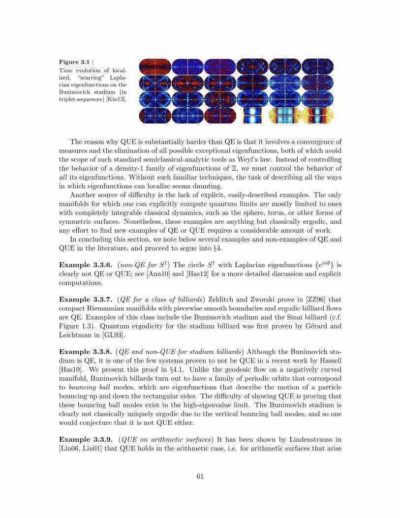
Figure 3.1 |Time evolution of local-ized, “scarring” Lapla-cian eigenfunctions on theBunimovich stadium (intriplet sequences) [Kin13].

The reason why QUE is substantially harder than QE is that it involves a convergence ofmeasures and the elimination of all possible exceptional eigenfunctions, both of which avoidthe scope of such standard semiclassical-analytic tools as Weyl’s law. Instead of controllingthe behavior of a density-1 family of eigenfunctions of Ξ, we must control the behavior ofall its eigenfunctions. Without such familiar techniques, the task of describing all the waysin which eigenfunctions can localize seems daunting.

Another source of difficulty is the lack of explicit, easily-described examples. The onlymanifolds for which one can explicitly compute quantum limits are mostly limited to oneswith completely integrable classical dynamics, such as the sphere, torus, or other forms ofsymmetric surfaces. Nonetheless, these examples are anything but classically ergodic, andany effort to find new examples of QE or QUE requires a considerable amount of work.

In concluding this section, we note below several examples and non-examples of QE andQUE in the literature, and proceed to segue into §4.

Example 3.3.6. (non-QE for S1) The circle S1 with Laplacian eigenfunctions einθ isclearly not QE or QUE; see [Ana10] and [Has12] for a more detailed discussion and explicitcomputations.

Example 3.3.7. (QE for a class of billiards) Zelditch and Zworski prove in [ZZ96] thatcompact Riemannian manifolds with piecewise smooth boundaries and ergodic billiard flowsare QE. Examples of this class include the Bunimovich stadium and the Sinai billiard (c.f.Figure 1.3). Quantum ergodicity for the stadium billiard was first proven by Gerard andLeichtman in [GL93].

Example 3.3.8. (QE and non-QUE for stadium billiards) Although the Bunimovich sta-dium is QE, it is one of the few systems proven to not be QUE in a recent work by Hassell[Has10]. We present this proof in §4.1. Unlike the geodesic flow on a negatively curvedmanifold, Bunimovich billards turn out to have a family of periodic orbits that correspondto bouncing ball modes, which are eigenfunctions that describe the motion of a particlebouncing up and down the rectangular sides. The difficulty of showing QUE is proving thatthese bouncing ball modes exist in the high-eigenvalue limit. The Bunimovich stadium isclearly not classically uniquely ergodic due to the vertical bouncing ball modes, and so onewould conjecture that it is not QUE either.

Example 3.3.9. (QUE on arithmetic surfaces) It has been shown by Lindenstrauss in[Lin06, Lin01] that QUE holds in the arithmetic case, i.e. for arithmetic surfaces that arise

61

as the quotient of the Poincare half-disk H by certain congruent co-compact lattices Γ.As mentioned in §1.1, this case is interesting because there exists a class of Laplacian-likeoperators, called Hecke operators, that share common eigenfunctions with the Laplacian.Nonetheless, arithmetic QUE is beyond the scope of this thesis, and we refer the interestedreader to [Mar06], [Sar11], and [Sou10].

Further examples and non-examples involve detailed computations. To gather a sense ofhow extensive these calculations are, we refer the reader to [Zel10], which works out thefailure of QE and QUE on the flat torus.

62

4 Recent Developments in Quantum Unique Ergodicity

In this largely expository final chapter, we discuss the intuition and heuristics behind Has-sell’s disproof of QUE for the Bunimovich stadium, a topic within the scope of our thesis.We then conclude with a brief survey of recent progress in QUE research on several fronts,some of which have already been mentioned. We will avoid technical details in all cases,and instead aim to explain how the advances we describe are significant.

4.1 No Quantum Unique Ergodicity on the Bunimovich Stadium

Hassell’s disproof of QUE on the Bunimovich stadium (and more generally, partially rect-angular surfaces) is the only known counterexample to QUE for billiard systems where thegeodesic flow exhibits “chaoticity” and the quantum dynamics are known to be QE [Bun79].Let us give a semi-formal definition of the Bunimovich stadium as follows:

Definition 4.1.1. (Bunimovich stadium) The Bunimovich stadium Xt is a 2-dimensionalRiemannian manifold formed by adjoining a rectangle with aspect ratio t to two circles.With normalization, it is given explicitly as ([−tπ/2, tπ/2]×[−π/2, π/2])∪Bπ/2((±tπ/2, 0)) ⊂R2, where Br(c) denotes the ball of radius r around center c.

As evidenced by Figure 1.3, billiards on Xt are unlike the geodesic flow on a negativelycurved manifold in the sense that the rectangular part of Xt gives rise to seemingly inte-grable dynamics: that is, billiards on Xt exhibit a family of 1-dimensional periodic orbitsthat correspond to billiards bouncing back and forth orthogonally against the rectangularwalls. As mentioned before, this is termed a bouncing ball mode, and “scarring” involvingthese modes was studied by Heller as early as 1984 [Hel84]. Although Xt is QE becausethese orbits form a set of (Liouville) measure zero, Xt fails to be QUE because they exist inthe high-eigenvalue limit. Hassell’s main result shows that some high-eigenvalue eigenstatesof Xt do indeed have a positive mass on the bouncing ball orbits. More specifically:

Theorem 4.1.2. (Hassell, [Has10]) For every ε > 0, there exists a subset Bε ⊂ [1, 2] ofmeasure at least 1 − 4ε and a constant m(ε) > 0 with the following property: for everyt ∈ Bε, there exists a quantum limit formed from Dirichlet eigenfunctions of ∆ on thestadium Xt that gives probability mass at least m(ε) to the bouncing ball trajectories.

Numerical computations, as well as construction of quasi-modes—approximate solutions foreigenfuctions given by Wentzel-Kramers-Brillouin (WKB) methods—had already indicatedbefore Hassell’s work that there exists a subsequence of modes whose Wigner measuresconverge to the singular measure supported on all bouncing balls. The main difficulty wasshowing that such bouncing ball modes exist in the limit: there may be many true eigen-functions whose eigenvalues are close to that of a given quasi-mode’s. In this regard, Hassellproves the theorem using a combination of the following techniques:

• the Heller-Zelditch argument, which already shows that eigenfunctions of ∆ localize onany Bunimovich stadium Xt, with the possible exception of those with eigenvalues inthe intervals [n2−O(1), n2+O(1)] for n ∈ Z. This is done using an explicit constructionof quasi-modes of the form vn = sin(ny)χ(x) or vn = cos(ny)χ(x), where χ(x) is some

63

Figure 4.1 |A bouncing ball mode (blue) andchaotic trajectory (red) on theBunimovich stadium Xt, for t ∈[1, 2]. The notation is describedin the text.

n

n

→

→/2

t/2

!!

π

π

suitable cutoff function. With vn defined as above, we see that ∆vn = n2vn + O(1),i.e. the spectrum of vn is concentrated in the interval [n2 −O(1), n2 +O(1)]. If thereare only O(1) eigenvalues in this interval, then it can be shown that eigenfunctionlocalization, or “scarring,” occurs in momentum space for these intervals. We referthe reader to [Tao08] and [ZZ96] for technical details about this argument.

The difficult task at the center of the proof is showing there are indeed only O(1)eigenfunctions in the interval [n2−O(1), n2 +O(1)] for n ∈ Z. Although the “standardtool” of Weyl’s law had too large an error term for this task, Hassell used the followingto achieve the necessary bound:

• the Hadamard variation formula, which details how the eigenvalues of Xt vary withthe aspect ratio of its rectangular component t. This is the equation

d

dtλk(t) = −

∫∂Xt

sgn(x)

2(Y · ~n)|∂~nϕk(x, t)|2ds,

where (ϕk, λk) is an eigenvector-eigenvalue pair of the Dirichlet Laplacian ∆ on Xt, ~nis the outward unit normal vector at ∂Xt, Y is the vector field which equals 1

2∂x on the

right semicircle of Xt, and ds is the length element on ∂Xt. Since sgn(x)2 (∂x · ~n) ≥ 0

everywhere, this formula tells us that the magnitude of the k-th eigenvalue alwaysdecreases as the aspect ratio t of Xt increases. This is consistent with Weyl’s lawon Xt (Corollary 2.3.15), which states λk = 4πk

Area(Xt)(1 + o(1)). Using the Hadamard

variation formula, Hassell shows the refinement

− d

dtλk(t) ∼ λk(t)

in expectation over k.

• the properties of quantum unique ergodicity, which allow a proof by contradiction.In particular, if Xt is QUE—the eigenfunctions equidistribute in the phase spaceT ∗Xt—then by Egorov’s theorem (Theorem 2.3.16), the positions and momenta ofeigenfunctions in T ∗Xt are propagated by the geodesic flow. Given billiard dynamics,however, we see that all geodesics on Xt intersect the boundary ∂Xt, and it can beshown that any equidistributed eigenfunction also has a normal derivative that isequidistributed on ∂Xt; see [Has10] and [Tao08] for a formalization of this argument.Thus, all eigenfunctions are equidistributed on ∂Xt, which implies that the exponentialdecay − d

dtλk(t) ∼ λk(t) holds for all eigenvalues λk and not just in expectation. Wecan then show rigorously that the eigenvalues of ∆ cannot conspire to concentrate

64

in any interval of the form [n2 − O(1), n2 + O(1)], n ∈ Z for most t ∈ [1, 2], elsethe eigenvalues “loiter” near the value n2 for significant intervals of t and contradictthe exponential decay condition above. The Heller-Zelditch argument then gives acontradiction to the QUE assumption, proving the desired statement.

It is interesting to note that billiards on the Bunimovich stadium is one of the few modelsystems for which we have a firm understanding of QE and QUE. There have been no furtherdisproofs of QUE on any billiard system since Hassell’s result, though it is currently believedthat QUE holds for billiards on the Barnett stadium (Figure 1.3). This is largely due to thework of Barnett, who verified QUE in this setting up to the 30,000th eigenfunction. Thoughit is a clear counterexample to QUE, the Bunimovich stadium illustrates the key themesof physical intuition and geometric visualization we mentioned in §1.3, and is therefore animportant model system to remember.

4.2 Frontiers in Semiclassical Analysis and Quantum Chaos

In concluding this thesis, we mention the following research areas on QUE and its relateddisciplines. As noted before, there are many works that lie completely outside the scope ofour thesis; see [Ana09, Non10, Sar11, Zel10] for more detailed surveys. Below, we aim toprovide a summary of several topics that lie within the scope of our exposition, so that thereader can readily pursue further research in the following areas.

Microlocal and semiclassical analysis. There are several areas of microlocal and semi-classical analysis relevant to PDE analysis; examples include heat kernel methods, Fourierintegral operators, the Fourier-Bros-Iagolnitzer (FBI) transform, and stationary phase ap-proximations. We refer the reader to [Dui95], [Mar02], and [Zwo12] for standard treatmentsof these topics. A survey of recent research in microlocal and semiclassical analysis can befound in [MU08] and [UW10].

Failure of QUE for cat maps. It is oftentimes useful to extend the ergodicity of thegeodesic flow to the ergodicity of any map on the symplectic phase space T ∗M , where(M, g) is a Riemannian manifold. Instead of a flow, “classical” dynamics may be providedby a discrete time transformation f : T ∗M → T ∗M that preserves the symplectic structure.Such maps can be reconstructed from flows by considering Poincare sections transversal tothe flow, and allow us to gain insight into such topics as hyperbolic symplectomorphisms onthe 2-dimensional torus. An explicit example of this subject is given by Arnold’s cat map(Figure 4.2a), defined by the action of the matrix

Γ =

(1 11 2

)on T2 = R2/Z2, i.e. fΓ : T2 3 (x, p) 7→ (x+ p, x+ 2p) mod 1 ∈ T2. It has been shown that,although such maps possess the Anosov (strongly chaotic) property, the analogue of QUEfor quantizations of hyperbolic toral symplectomorphisms fails to hold. This suggests thatthere may be something unique about the geodesic flow on a negatively curved manifold,and perhaps the QUE conjecture (Conjecture 3.3.5) is already the best possible statementone can hope for. The reader may consult [FNdB03] and [FN04] for further reading.

65

Figure 4.2 |Illustrationsfor two cur-rent researchareas in QUE.

(a) A graphical representation of Arnold’s catmap, the model hyperbolic toral symplecto-morphism. Aside from being a test case forQUE, it is also used in dynamical systems the-ory and image processing.

(b) A numerically-computed densityplot of |ϕn|2 on the Barnett stadium,where n ≈ 5× 104 and λn ≈ 106, as cal-culated by Barnett’s method in [Bar06].

Numerical simulations of QUE. Given the technical difficulty of proving the QUE con-jecture outright, many researchers have been interested in finding numerical evidence forit. The most notable project is Barnett’s simulation of 30,000 eigenfunctions of the Bar-nett billiard (Figure 4.2b), a uniformly hyperbolic planar Euclidean billiard system, whichproduced evidence that QUE holds in this case. Barnett studied the rate of equidistribu-tion of Dirichlet eigenfunctions of ∆ on the Barnett stadium by examining the diagonalsof the matrix elements 〈ϕn, Aϕm〉, where A is some suitably defined test ψDO and ϕn isan eigenfunction of ∆ with eigenvalue λn. In using an efficient scaling method to computethese quantities up to n,m ≈ 7× 105, Barnett found that his sample variance decayed witheigenvalue magnitude as a power of 0.48 ± 0.01, and demonstrated a 102 improvement ofeigenvalue magnitude over previous studies. We refer the reader to [Bar06], [Bar14], and[Non10] for a more detailed treatment of this topic.

Spectral statistics. This tangentially-related area deals with the inverse problem of de-scribing the geometric information we obtain from the eigenpairs of ∆ using tools fromfields such as random matrix theory. Although it is rarely possible to explicitly write thespectral information of ∆ on any domain, one may hope to gain statistical and asymp-totic information about the eigenpairs given detailed knowledge of the classical billiard orgeodesic flow. Weyl’s law (Corollary 2.3.15) is an example of how this can be done: ittells us that as λ → ∞, the counting function N(λ) = #λn ≤ λ satisfies the asymp-

totic relation N(λ) ∼ Area(Ω)4π λ, where Ω is a planar Euclidean domain. In the same way

that the area of Ω determines the asymptotic mean density of eigenvalues, we may intro-duce the consecutive level spacing distribution as a function that counts the fraction ofeigenvalues λn less than λ, whose distance from the next eigenvalue λn+1 is less than s:P (s,N) := 1

N

∑Nj=1 1(s > λn+1 − λn). If the sequence λn is sufficiently “randomized,”

then there should exist a limit distribution P (s) = limN→∞ P (s,N) so that

limN→∞

∫ ∞0

P (s,N)h(s)ds =

∫ ∞0

P (s)h(s)ds.

66

for any nice function h. The 1977 Berry-Tabor conjecture, which has been proven in manycases, asserts that for “generic integrable systems” the limit distribution P (s) is equal to thewaiting-time distribution for a Poisson process (i.e. P (s) = exp(−s)) [Ber89]. On the otherhand, for “generic” systems with an ergodic geodesic flow the 1984 Bohigas-Giannoni-Schmidt conjecture proposes that the limit distribution P (s) is equal to the consecutivelevel spacing distribution of a suitable Gaussian ensemble of Hermitian random variables[BGS84]. Numerical experiments have shown that the eigenvalue spacing statistics for theSinai billiard correspond to those of the Gaussian orthogonal ensemble (GOE) distribution[BK10, Rud08]. One hopes that studying these statistics will lead to an increased under-standing between how integrable and chaotic systems differ in the semiclassical limit.

Other research areas. Aside from the topics mentioned above, there has also beenprogress in QUE research in the general case for negatively curved manifolds, which isexemplified in Anantharaman and Nonnenmacher’s lower bound on the “entropy” of anyquantum limit on such manifolds [Ana08, AN07, Ana10]. This implies that quantum lim-its cannot be too localized, although the result does not prevent the limits from havingsome highly localized ergodic components. Finally, another major result in QUE researchis the proof of QUE in the arithmetic case; see Example 3.3.9 for a brief discussion ofLindenstrauss’s work.

4.3 Conclusion

We end this thesis with a review of the semiclassical tools and results on quantum ergodic-ity we have developed, before proceeding to discuss the relevance of what we have hithertostudied and the future of quantum chaos at large. Having started from first principles indifferential and symplectic geometry, we formalized the Laplace-Beltrami operator, moti-vated the study of quantum chaos—and in particular, the questions of quantum ergodicityand quantum unique ergodicity—and addressed these topics by developing the fundamentaltools of semiclassical analysis. These results include the notion of Weyl quantization, whichrelates a function defined on phase space to a self-adjoint operator acting on functions in con-figuration space; the symbol calculus, which formalizes the analytic and algebraic propertiesof Weyl-quantized pseudodifferential operators; Weyl’s law, which controls the asymptoticmean density and behavior of the eigenvalues of a generalized Hamiltonian operator orLaplacian; and Egorov’s theorem, which relates the classical time evolution given by thegeodesic flow on a manifold to the quantum-mechanical time evolution given by a unitarypropagator. We then proved the quantum ergodicity theorem of Schnirelman, Zelditch, andde Verdiere using a combination of the symbol calculus, Weyl’s law, and Egorov’s theorem,after which we rigorously formulated the quantum unique ergodicity conjecture and brieflydiscussed current research areas in quantum chaos.

As we have mentioned before, our approach to semiclassical analysis and quantum er-godicity emphasizes intuition over straightforward proofs. The key themes introduced in§1.3, which serve as general guidelines for thinking about problems related to semiclassi-cal analysis and quantum chaos, illustrate this approach. For instance, we have seen thatthe billiard flow serves as a model dynamical system whose trajectories may be regular orchaotic depending on the geometry of the domain, and that the classical-quantum corre-spondence provides a physical heuristic as to when the QE property may hold. It is also

67

important to stress that the tools we have developed in this thesis find broader applica-tions beyond QE and QUE. In regard to semiclassical analysis, we can apply such notionsas Weyl quantization and Garding’s inequality to the analysis of PDEs. On the quantumchaos side, we may examine direct applications of Egorov’s theorem to problems in quantummechanics, as well as model the behavior of h-dependent and chaotic Hamiltonians. Lastly,in considering spectral statistics, we can endeavor to relate the distributional properties ofLaplacian eigenvalues to the classical behaviors of corresponding systems. References forthe foregoing applications have been mentioned in §4.2.

Let us now step backwards and examine QE and QUE as they relate to other fields.Our predominant emphasis on QE begs the question of how relevant QE is as a physicalconcept. Why, in particular, do we care that eigenfunctions of the Laplacian equidistribute?How physically useful are the notions of QE and QUE, and why should we study themif statements like the QUE conjecture are seemingly so far out of reach? The answer istwofold. The one appealing to most mathematicians is that QE leads to, and is inspiredby, many beautiful mathematical theories, some of which (like semiclassical analysis) havefound broader utility which justifies their development. The second answer, which appealsto most physicists and pragmatists, is that the subject may find applications in condensedmatter or quantum physics. For example, the basic idea of ergodicity is used in statisticalmechanics as a measure of how chaotic and mixing an ensemble of particles is, and mayalso serve as a factor influencing the higher-level material properties of a system. Chaoticeffects are manifest in atomic systems where a particle can roam freely, as in electron scat-tering. Heat kernel methods, which are related to semiclassical analysis, can be computedusing Feynman path integrals as expansions over geodesic terms [Bar12]. Other areas ofapplication include wavepacket dynamics and many-body systems; the equidistribution ofeigenfunctions may be important here if we specifically want particles to scar disjoint sub-spaces of the configuration manifold, so that they become well-described by stable periodicorbits. It may even be argued that chaotic—as opposed to regular—systems are the breadand butter of science: in nature, nothing is ever ideal, and the classical dynamics of asystem are almost never completely integrable.

Although the resolution of the QUE conjecture seems to lie beyond the range of ourcurrent techniques, a full proof or disproof of the QUE conjecture for negatively curvedmanifolds would undoubtedly lead to new insights into quantum mechanics, and may in-troduce new techniques applicable to other areas of analysis and geometry. In aiming toformulate the questions of quantum ergodicity and quantum unique ergodicity, it is ourhope that the mathematics developed in this thesis will contribute toward an increasedunderstanding of semiclassical analysis and quantum chaos.

68

Appendices

Appendix I: Results from Functional Analysis

In this appendix, we provide a summary of the functional-analytic tools needed to addressthe Laplacian, which are also used in proofs throughout the thesis. A basic backgroundin functional analysis is assumed; more detailed treatments than the one we present belowcan be found in standard analysis textbooks. See, for example, [dMG81], [Dav95], [Hel10],[Hor83a], [Hor83b], [RS80], and [SS11].

Recall that a topological space S is said to be separable if it contains a countable, densesubset, i.e. there exists a sequence xn∞n=1 of elements of S such that every nonemptyopen subset of S contains at least one element of xn∞n=1. Let (H, 〈·, ·〉) denote a separablecomplex Hilbert space. We remind ourselves that the spectrum of a bounded linear operatorT : H → H is given by the set of all λ such that T − λI has a kernel. (T is bounded ifits operator norm, written below, is finite.) λ ∈ Spec(T ) is an eigenvalue of T if ∃x 6= 0 :Tx = λx. Recall as well that T is compact if it maps a bounded set of H to a relativelycompact (the closure is compact) subset of H. The space of compact operators forms aclosed ideal in the space of bounded operators in the topology induced by the operatornorm ||T || = minc ≥ 0 : ||Tx|| ≤ c||x|| ∀x ∈ H: in particular, if T is compact andS is bounded, then TS and ST are also compact; if there is a sequence Tn such that||Tn − T || → 0 as n→∞ and the Tn’s are all compact, then T is also compact.

The adjoint of T : H → H is the operator T ∗ satisfying 〈Tx, y〉 = 〈x, Ty〉 for x, y ∈ H.T is said to be self-adjoint if T = T ∗. The standard spectral theorem for a bounded self-adjoint operator T : H → H, which is proven in [Dav95, RS80], states that there is anorthonormal basis of H consisting of eigenvectors of T with real eigenvalues. The analoguefor unbounded operators is more complicated, and requires some technical detail to get right.

Theorem I.1. (spectral theorem for bounded operators) For each self-adjoint boundedoperator T : H → H, there exists a measure space (X,A, µ), a real-valued functionf ∈ L∞(X,µ), and a unitary operator U : H → L2(X,µ) such that U∗MfU = A, thereMf : x 7→ fx for x ∈ L2(X,µ) is the multiplication operator.

Theorem I.2. (spectrum of self-adjoint operators) If T : H → H is a self-adjoint boundedoperator, then (T − λI)−1 exists and is a bounded linear operator on H for all λ ∈C/Spec(T ), and if Spec(T ) ⊂ [c,∞), then 〈Tx, x〉 ≥ c||x||2 for x ∈ H.

Proofs of these two theorems can also be found in [RS80] and [SS11].

Now recall that an unbounded operator S : H → H is a linear operator defined on a sub-space D(S) ⊂ H called the domain of S; in particular, S is a linear transformation fromD(S) → H. S is said to be densely defined in D(S) is dense as a subset in H. The graphof S is defined as the set G(S) := (x, Sx) : x ∈ D(S) ⊂ H ×H, and S is closed if G(S) isa closed subspace of H ×H with norm ||(x, y)||2 = ||x||2 + ||y||2. S is closable if there is aclosed unbounded operator S s.t. D(S) ⊆ D(S) and L = S on D(S). A standard result offunctional analysis is that S is uniquely defined; call it the closure of S.

If S is a unbounded densely defined operator, then it always has an unbounded adjoint

69

operator S∗ such that 〈S∗x, y〉 = 〈x, Ly〉 for all x ∈ D(S∗), y ∈ D(S), where D(S) = y ∈H : |〈Sx, y〉| ≤ Cy||x|| ∀x ∈ D(S). Furthermore, S∗ is always closed, and if it is denselydefined, then S is closable with S = (S∗)∗, S

∗= S∗. See [SS11] for a proof of this assertion.

Finally, we recall that an unbounded, densely defined operator S : H → H is symmetric if〈Sx, y〉 = 〈x, Sy〉 for all x, y ∈ D(S); i.e. S ⊆ S∗, where S ⊆ S∗ means that D(S) ⊆ D(S∗)and S = S∗ on all x ∈ D(S). S is self-adjoint if S = S∗, and if S is symmetric, then it isessentially self-adjoint if S = S∗.

In the form of a multiplication operator, the spectral theorem for unbounded operatorscan be stated as follows:

Theorem I.3. (spectral theorem for unbounded operators) For each self-adjoint unboundedoperator S : H → H, there exists a measure space (X,A, µ), a real-valued measurable func-tion f , and a unitary operator U : H → L2(X,µ) such that x ∈ D(S) iffMf (Ux) ∈ L2(X,µ),and x ∈ D(L) =⇒ U(Ax) = Mf (Ux), where Mf : x 7→ fx is the (unbounded) multiplica-tion operator on X.

Proofs of this result can be found in [Dav95], [RS80], and [SS03].

Note that the Laplace-Beltrami operator on H = L2(M) is densely defined, with domainC∞c (M). This can be seen with an application on the closed graph theorem, which, albeitstandard functional analysis-fare, will not be presented here.

Let us state several more theorems used in proofs of other results throughout our the-sis. One useful result from functional analysis is Stone’s theorem on one-parameter unitarygroups, which establishes a one-to-one correspondence between self-adjoint operators on Hand one-parameter families U(t), t ∈ R of unitary operators that are both strongly contin-uous and are homomorphisms. More precisely:

Theorem I.4. (Stone) If T : D(T )→ H is a bounded or unbounded self-adjoint operator,then U(t) := exp(−itT ) for t ∈ R is a strongly continuous unitary group of homomorphisms,i.e.

∀t0 ∈ R, x ∈ H, limt→t0

U(t)x = U(t0)x

and∀s, t ∈ R, U(t+ s) = U(t)U(s), U(t)∗ = U(−t).

Furthermore, we have ddt(U(t)x) + U(t)Tx = 0 for all t ∈ R and x ∈ H. If there is a group

of unitary operators satisfying the continuity and homomorphism conditions above, thenwe can also produce a self-adjoint operator T such that all the conditions above hold.

A proof of Stone’s theorem can be found in [RS80] and [SS11]. We also prove the followingtheorem for reference:

Theorem I.5. (inverses of bounded linear operators) Let X and Y be Hilbert spaces,A : X → Y be a bounded linear operator, and B1, B2 : Y → X be bounded linear operatorssatisfying

AB1 = I + C1 and B2A = I + C2,

70

where C1 : Y → Y , C2 : X → X, ||C1|| < 1, and ||C2|| < 1. Then there exists A−1 : Y →X : AA−1 = A−1A = I.

Proof. Note that, since ||C1|| < 1,∑∞

i=0(−1)iCi1 converges and is an inverse to theoperator I + C1. Thus AA0 = I, where A0 := B1(I + C1)−1. Similarly, A1A = I whereA1 := (I+C2)−1B2. Since A has both a left and right inverse, from basic functional analysiswe know that it is invertible with A−1 = A0 = A1.

Let us end the appendix by citing two useful theorems from [Zwo12]. These results areneeded in the proofs of Theorems 2.2.16 (inverses for elliptic symbols) and 2.3.3 (Weyl’slaw). The first theorem gives an explicit expression for the eigenvalues of any suitable self-adjoint operator, while the second theorem deals primarily with bounding the eigenvaluecounting function N(λ), adapted for operators beyond ∆.

Theorem I.6. (Courant-Fischer) Let T : H → H be a self-adjoint operator with 〈Tx, x〉 ≥c〈x, x〉, and suppose that the right inverse (T −2c)−1 : H → H is a compact operator. ThenSpec(T ) is discrete and countable, and D(T ) = (T − 2c)−1H. If we order the eigenvaluesin ascending order as λ1 ≤ λ2 ≤ ..., then we also have

λj = maxV⊂H

dimV <j

minw∈D(T )

dimw⊥V 6=0

〈Tw,w〉||w||2

= minV⊂D(T )dimV≥j

maxw∈Vw 6=0

〈Tw,w〉||w||2

,

where V is a linear subspace of H.

The proof of Theorem I.6 can be found in [RS80, CH89]. For the following statement, letrank T = dimT (H), where T : H → H is a bounded linear operator. If S : H → H is anoperator that possesses a real and discrete spectrum, then we set NS(λ) := #λn : λn ≤ λ.

Theorem I.7. (estimates of N(λ)) Let T : H → H be a self-adjoint operator with〈Tx, x〉 ≥ c〈x, x〉, and suppose that the right inverse (T − 2c)−1 : H → H is a compactoperator.

(i) If there exists some δ > 0 and an operator S : D(T )→ H with rank ≤ k such that

〈Tx, x〉 ≥ (λ+ δ)||x||2 − 〈Sx, x〉

for x ∈ D(T ), then NT (λ) ≤ k.(ii) If for all δ > 0 there exists a subspace V ⊂ D(T ) with dimV ≥ k such that

〈Tx, x〉 ≤ (λ+ δ)||x||2

for x ∈ V , then NT (λ) ≥ k.

The proof of Theorem I.7 uses Theorem I.6, and can be found in [Zwo12].

71

Appendix II: Quantization Formulas and Proof of the Expansion Theorem

We compile the following quantization procedures, for a = a(x, p) ∈ S(R2n) being a real-valued symbol:

Quantization Formula

Weyl quantization Opw(a)(ϕ)(x) = (2πh)−n∫∫

Rn×Rn eih〈x−y,p〉a

(x+y

2, p)ϕ(y)dydp

left (standard) quantization Opl(a)(ϕ)(x) = (2πh)−n∫∫

Rn×Rn eih〈x−y,p〉a(x, p)ϕ(y)dydp

right quantization Opr(a)(ϕ)(x) = (2πh)−n∫∫

Rn×Rn eih〈x−y,p〉a(y, p)ϕ(y)dydp

t-quantization, t ∈ [0, 1] Opt(a)(ϕ)(x) = (2πh)−n∫∫

Rn×Rn eih〈x−y,p〉a(tx+ (1− t)y, p)ϕ(y)dydp

Table 1 | A compilation of quantization procedures

The properties of Weyl quantization are discussed in §2.1.2 and §2.2. The following ta-ble lists explicit formulas for the quantizations of certain symbols, as shown in examplesthroughout the thesis (c.f. Appendix VI):

Symbol Quantization Location

pα Opt(a)(ϕ)(x) = a(x, hD)ϕ(x) = (hD)αϕ(x) Example 2.1.15∑|α|≤N aα(x)pα Opt(a)(ϕ)(x) = a(x, hD)ϕ(x) =

∑|α|≤N aα(x)(hD)αϕ(x) Example 2.1.15

〈x, p〉 Opt(a)(ϕ) = (1− t)〈hD, xϕ〉+ t〈x, hDϕ〉Opw(a)(ϕ) = h

2(〈D,xϕ〉+ 〈x,Dϕ〉) Example 2.1.16

a(x) Opt(a)(ϕ) = aϕ Example 2.1.17〈x, x∗〉+ 〈p, p∗〉 Opt(a) = 〈x, x∗〉+ 〈hD, p∗〉 Example 2.1.18

eih〈x,x∗〉+〈p,p∗〉 Opw(a)(x, hD) = e

ihl(x,hD) Lemma 2.2.1

Table 2 | A compilation of quantization examples

We devote the remainder of this appendix to proving Theorem 2.2.6 (semiclassical expan-sion), following the proof in [Zwo12].

Lemma II.1 (quadratic phase asymptotics, [Zwo12]) Let Q be an invertible, symmetric realmatrix. Then for each N ∈ Z+, we have∫

Rnei

2h〈Qx,x〉a(x)dx = (2πh)n/2

eiπ4

sgn(Q)

| detQ|1/2

(N−1∑k=0

hk

k!

(〈Q−1D,D〉

2i

)ka(0) +O(hN )

),

where a ∈ C∞c (Rn) is real-valued.Proof. We combine Proposition 2.1.9 and Plancherel’s theorem to see that∫

Rnei

2h〈Qx,x〉a(x)dx =

(h

2π

)n/2 eiπ4

sgn(Q)

| detQ|1/2

∫Rne−

ih2〈Q−1p,p〉a(p)dp.

Setting I(h, a) :=∫Rn exp(− ih

2 〈Q−1p, p〉)a(p)dp, we see that

∂I(h, a)

∂h=

∫Rne−ih

2〈Q−1p,p〉

(− i

2〈Q−1p, p〉a(p)

)dp = I(h, Pa),

72

where P = − i2〈Q

−1D,D〉. Thus

I(h, a) =

N−1∑k=0

hk

k!I(0, P ka) +

hN

N !RN (h, a),

where RN (h, a) is the remainder term given by

Rn(h, a) = N

∫ 1

0(1− t)N−1I(th, PNa)dt.

Applying the Fourier inversion identity gives

I(0, P ka) =

∫Rn

(− i

2〈Q−1p, p〉

)ka(p)dp = (2π)nP ka(0),

and using Proposition 2.1.5 gives a bound on the remainder as

|RN | ≤ CN ||PNa||1 ≤ CN sup|α|≤2N+n+1

|∂αa|,

as desired.

Proposition II.2 (stationary phase formula, [Zwo12]) If a ∈ C∞c (R4n), then∫∫R2n×R2n

eihσ(z,w)a(z, w)dzdw = (2πh)2n

(N−1∑k=0

hk

k!

(σ(Dx, Dp, Dy, Dq)

i

)ka(0, 0) +O(hN )

)

for each N ∈ Z+, where z = (x, p) ∈ R2n and w = (y, q) ∈ R2n.Proof. Let

Q =

(−J

J

).

As in Lemma 2.2.4, we see that 12〈Q(z, w), (z, w)〉 = σ(z, w) and

1

2〈Q−1D,D〉 = σ(Dx, Dp, Dy, Dq).

Applying Lemma II.1 above gives the result.

Proof of Theorem 2.2.6. The main idea of this proof is to use Proposition II.2 abovebut take h/2 instead of h and −σ instead of σ, and substitute this into the integral repre-sentation formula (Theorem 2.2.5). Thus, if a, b ∈ S, then

(f#g)(x, p) = (πh)−2n

∫∫R2n×R2n

e−2ihσ(w1,w2)a(z + w1)b(z + w2)dw1dw2,

where z = (x, p). It remains to show that the remainders are in OS(hN+1). For that wenote from the composition theorem that

eihA(D) =

N∑k=0

(ih)k

k!A(D)k +

iN+1hN+1

N !

∫ 1

0(1− t)NeithA(D)A(D)N+1dt,

73

where eithA(D)A(D)N+1 is multiplication by F−1eitA(ζ)A(ζ)N+1F (where F is the Fouriertransform and ζ ∈ R4n). Hence eithA(D)A(D)N+1 : S(R4n)→ S(R4n) uniformly in h and t,which proves the estimate on the remainder. For the other equations, we simply compute

a#b = ab+ ihA(D)(a(x, p)b(x, p)|y=x,q=p +O(h2)

= ab+ih

2(〈Dpa,Dyb〉 − 〈Dxa,Dqb〉)|y=x,q=p +O(h2)

= ab+h

2i(〈∂pa, ∂xb〉 − 〈∂xa, ∂pb〉) +O(h2) = ab+

h

2ia, b+O(h2).

and

[Opw(a), Opw(b)] = Opw(a)Opw(b)−Opw(b)Opw(a) = Opw(a#b− b#a)

= Opw(ab+

h

2ia, b+

h2

2A(D)2(ab)|y=x,q=p +OS(h3)

)−Opw

(ba+

h

2ib, a+

h2

2A(D)2(ba)|y=x,q=p +OS(h3)

)=

h

iOpw(a, b) +Opw(OS(h3)),

where the final equality follows because

(A(D)2(a(x, p)b(y, q))−A(D)2(b(x, p)a(y, q)))|y=x,q=p = 0.

Finally, if supp(a) ∩ supp(b) = ∅, then each term in the expansion above vanishes forarbitrary N . This gives the result.

74

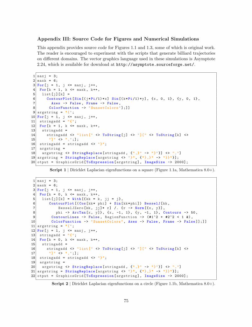
Appendix III: Source Code for Figures and Numerical Simulations

This appendix provides source code for Figures 1.1 and 1.3, some of which is original work.The reader is encouraged to experiment with the scripts that generate billiard trajectorieson different domains. The vector graphics language used in these simulations is Asymptote2.24, which is available for download at http://asymptote.sourceforge.net/.

1 maxj = 3;

2 maxk = 6;

3 For[j = 1, j <= maxj , j++,

4 For[k = 1, k <= maxk , k++,

5 list[j][k] =

6 ContourPlot[Sin[(j*Pi/1)*x] Sin[(k*Pi/1)*y], x, 0, 1, y, 0, 1,

7 Axes -> False , Frame -> False ,

8 ColorFunction -> "SunsetColors"];]]

9 argstring = "";

10 For[j = 1, j <= maxj , j++,

11 stringadd = "";

12 For[k = 1, k <= maxk , k++,

13 stringadd =

14 stringadd <> "list[" <> ToString[j] <> "][" <> ToString[k] <>

15 "]" <> ",";];

16 stringadd = stringadd <> "";

17 argstring =

18 argstring <> StringReplace[stringadd , "," -> ""] <> ","]

19 argstring = StringReplace[argstring <> "", "," -> ""];

20 otput = GraphicsGrid[ToExpression[argstring], ImageSize -> 2000];

Script 1 | Dirichlet Laplacian eigenfunctions on a square (Figure 1.1a, Mathematica 8.0+).

1 maxj = 3;

2 maxk = 6;

3 For[j = 1, j <= maxj , j++,

4 For[k = 0, k <= maxk , k++,

5 list[j][k] = With[kk = k, jj = j,

6 ContourPlot [(Cos[kk* phi] + Sin[kk*phi]) BesselJ[kk ,

7 BesselJZero[kk, jj]* r] /. r -> Norm[x, y],

8 phi -> ArcTan[x, y], x, -1, 1, y, -1, 1, Contours -> 50,

9 ContourLines -> False , RegionFunction -> (#1^2 + #2^2 < 1 &),

10 ColorFunction -> "SunsetColors", Axes -> False , Frame -> False ]];]]

11 argstring = "";

12 For[j = 1, j <= maxj , j++,

13 stringadd = "";

14 For[k = 0, k <= maxk , k++,

15 stringadd =

16 stringadd <> "list[" <> ToString[j] <> "][" <> ToString[k] <>

17 "]" <> ",";];

18 stringadd = stringadd <> "";

19 argstring =

20 argstring <> StringReplace[stringadd , "," -> ""] <> ","]

21 argstring = StringReplace[argstring <> "", "," -> ""];

22 otput = GraphicsGrid[ToExpression[argstring], ImageSize -> 2000];

Script 2 | Dirichlet Laplacian eigenfunctions on a circle (Figure 1.1b, Mathematica 8.0+).

75

1 if(! settings.multipleView) settings.batchView=false;

2 settings.tex="pdflatex";

3 defaultfilename="rectangle";

4 if(settings.render < 0) settings.render =4; settings.outformat="";

5 settings.inlineimage=true; settings.embed=true; settings.toolbar=false;

6 viewportmargin =(2,2); import graph; size (200);

7

8 path bill = (-50,-30) --(50,-30) --(50,30) --(-50,30)--cycle;

9 real phi = 2*pi *0.123456;

10 draw(bill);

11 pair s = (20 ,20), db, dt = exp(I*phi), e = s+200*dt;

12 path traj = s--e;

13 real [] c;

14

15 for(int i=0; i<50; ++i)

16 c = intersect(bill , traj);

17 e = point(traj , c[1]);

18 db = dir(bill , c[0]);

19 draw(s--e,red);

20 dot(e,blue);

21 dt = -dt + 2*dot(dt ,db)*db;

22 s = e;

23 e = s + 200*dt;

24 traj = (s+dt)--e;

25

Script 3 | Rectangle billiard trajectories (Figure 1.3a, Asymptote 2.24).

1 if(! settings.multipleView) settings.batchView=false;

2 settings.tex="pdflatex";

3 defaultfilename="circle";

4 if(settings.render < 0) settings.render =4; settings.outformat="";

5 settings.inlineimage=true; settings.embed=true; settings.toolbar=false;

6 viewportmargin =(2,2); import graph; size (200);

7

8 path bill = Circle ((0,0) ,90.0);

9 real phi = 2*pi *0.23456;

10 draw(bill);

11 pair s = (20 ,20), db, dt = exp(I*phi), e = s+200*dt;

12 path traj = s--e;

13 real [] c;

14

15 for(int i=0; i<50; ++i)

16 c = intersect(bill , traj);

17 e = point(traj , c[1]);

18 db = dir(bill , c[0]);

19 draw(s--e,red);

20 dot(e,blue);

21 dt = -dt + 2*dot(dt ,db)*db;

22 s = e;

23 e = s + 200*dt;

24 traj = (s+dt)--e;

25

Script 4 | Circle billiard trajectories (Figure 1.3b, Asymptote 2.24).

76

1 if(! settings.multipleView) settings.batchView=false;

2 settings.tex="pdflatex";

3 defaultfilename="bunimovich";

4 if(settings.render < 0) settings.render =4; settings.outformat="";

5 settings.inlineimage=true; settings.embed=true; settings.toolbar=false;

6 viewportmargin =(2,2); import graph; size (200);

7

8 path bill = (-50,-50) --(50,-50)--arc ((50 ,0), 50, -90, 90)

9 --(50,50) --(-50,50)--arc((-50,0), 50, 90, 270) --cycle;

10 real phi = 2*pi *0.123456;

11 draw(bill);

12 pair s = (20 ,20), db, dt = exp(I*phi), e = s+200*dt;

13 path traj = s--e;

14 real [] c;

15

16 for(int i=0; i<50; ++i)

17 c = intersect(bill , traj);

18 e = point(traj , c[1]);

19 db = dir(bill , c[0]);

20 draw(s--e,red);

21 dot(e,blue);

22 dt = -dt + 2*dot(dt ,db)*db;

23 s = e;

24 e = s + 200*dt;

25 traj = (s+dt)--e;

26

Script 5 | Bunimovich billiard trajectories (Figure 1.3c, Asymptote 2.24).

1 if(! settings.multipleView) settings.batchView=false;

2 settings.tex="pdflatex";

3 defaultfilename="sinai";

4 if(settings.render < 0) settings.render =4; settings.outformat="";

5 settings.inlineimage=true; settings.embed=true; settings.toolbar=false;

6 viewportmargin =(2,2); import graph; size (200);

7

8 path bill = (-90,-90) --(90,-90) --(90,90) --(-90,90)--cycle;

9 path inner = reverse(Circle ((0,0) ,30.0));

10 real phi = 2*pi *0.05;

11 filldraw(bill^^inner ,lightgray ,black);

12 pair s = (30 ,30), db, dt = exp(I*phi), e = s+200*dt;

13 path traj = s--e;

14 real [] co;

15 real [][] ci;

16

17 for(int i=0; i<20; ++i)

18 co = intersect(traj , bill);

19 ci = intersections(traj , inner);

20 if(ci.length > 0)

21 e = point(traj , ci [0][0]);

22 db = dir(inner , ci [0][1]);

23 else

24 e = point(traj , co[0]);

25 db = dir(bill , co[1]);

26

27 draw(s--e,red);

77

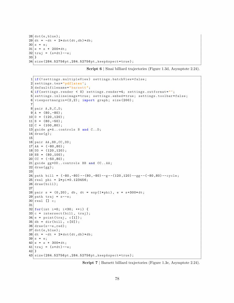
28 dot(e,blue);

29 dt = -dt + 2*dot(dt ,db)*db;

30 s = e;

31 e = s + 200*dt;

32 traj = (s+dt)--e;

33

34 size (284.52756pt ,284.52756pt ,keepAspect=true);

Script 6 | Sinai billiard trajectories (Figure 1.3d, Asymptote 2.24).

1 if(! settings.multipleView) settings.batchView=false;

2 settings.tex="pdflatex";

3 defaultfilename="barnett";

4 if(settings.render < 0) settings.render =4; settings.outformat="";

5 settings.inlineimage=true; settings.embed=true; settings.toolbar=false;

6 viewportmargin =(2,2); import graph; size (200);

7

8 pair A,B,C,D;

9 A = (80,-80);

10 D = (120 ,120);

11 B = (80,-50);

12 C = (100 ,80);

13 guide g=A.. controls B and C..D;

14 draw(g);

15

16 pair AA,BB,CC,DD;

17 AA = (-80,80);

18 DD = (120 ,120);

19 BB = (80 ,100);

20 CC = (-50,80);

21 guide gg=DD.. controls BB and CC..AA;

22 draw(gg);

23

24 path bill = (-80,-80) --(80,-80)--g- -(120 ,120) --gg --(-80,80) --cycle;

25 real phi = 2*pi *0.123456;

26 draw(bill);

27

28 pair s = (0 ,20), db , dt = exp(I*phi), e = s+300*dt;

29 path traj = s--e;

30 real [] c;

31

32 for(int i=0; i<30; ++i)

33 c = intersect(bill , traj);

34 e = point(traj , c[1]);

35 db = dir(bill , c[0]);

36 draw(s--e,red);

37 dot(e,blue);

38 dt = -dt + 2*dot(dt ,db)*db;

39 s = e;

40 e = s + 300*dt;

41 traj = (s+dt)--e;

42

43 size (284.52756pt ,284.52756pt ,keepAspect=true);

Script 7 | Barnett billiard trajectories (Figure 1.3e, Asymptote 2.24).

78

1 if(! settings.multipleView) settings.batchView=false;

2 settings.tex="pdflatex";

3 defaultfilename="triangle";

4 if(settings.render < 0) settings.render =4; settings.outformat="";

5 settings.inlineimage=true; settings.embed=true; settings.toolbar=false;

6 viewportmargin =(2,2); import graph; size (200);

7

8 path bill = (-80,-80) --(120,-80) --(-80,80)--cycle;

9 real phi = 2*pi *0.123456;

10 draw(bill);

11

12 pair s = (-70,0), db , dt = exp(I*phi), e = s+300*dt;

13 path traj = s--e;

14 real [] c;

15

16 for(int i=0; i<60; ++i)

17 c = intersect(bill , traj);

18 e = point(traj , c[1]);

19 db = dir(bill , c[0]);

20 draw(s--e,red);

21 dot(e,blue);

22 dt = -dt + 2*dot(dt ,db)*db;

23 s = e;

24 e = s + 300*dt;

25 traj = (s+dt)--e;

26

27 size (284.52756pt ,284.52756pt ,keepAspect=true);

Script 8 | Triangle billiard trajectories (Figure 1.3f, Asymptote 2.24).

As mentioned in §4.2, Barnett’s recent numerical computation of the eigenfunctions andeigenvalues of the Dirichlet Laplacian on the Barnett stadium is a notable work. A listof the first 62,076 eigenvalues in the range [0, 1276900] is available at http://www.math.

dartmouth.edu/~ahb/qugrs_n62076.Es.

79

Appendix IV: Index of Notation

List of symbols, in alphabetical order

1S ,1(S) indicator function of the setor event S

60

a a symbol 35A Weyl-quantization of a 36A σ-algebra 18A(D) the differential operator

12σ(Dx, Dp, Dy, Dq)

35

||A||L2→L2 operator norm of A : L2 →L2

37

Area(D) area of a Euclidean domainD ⊂ Rn

4

B∗ adjoint of an operator B 54Br(c) ball of radius r around c 63〈B〉T time-average of an operator

B55

C complex numbers 7C1(M) space of continuously differ-

entiable functions on M8

C∞(M) space of smooth functions onM

8

C∞c (M) space of smooth, compactlysupported functions on M

10

CP complex projective space 20Dx directional derivative with

respect to x35

Dαx

1

i|α|∂α 23

D′(M) space of all distributions onM

45

Dψ dispersion of a function ψ ∈L2(R)

27

∂n, ∂xn partial derivative in the nthlocal coordinate

8

∂β∏ni=1

∂βi

∂xβii

22

dxi basis coordinates for thecotangent space

9

∆,∆g,∆Ω Laplace-Beltrami operator,with dependencies on theRiemannian metric g anddomain Ω

7

∆D,∆N Laplace-Beltrami operatorwith Dirichlet and Neumannboundary conditions

8

δxy Dirac delta of x− y 8δ, δ(x) Dirac delta of x 24Diff(M) space of all C∞ diffeomor-

phisms of M45

dim dimension 15div divergence 8En energy level (eigenvalue of

∆) indexed by n13

exp(x) exponential map∑∞n=1

1n!xn 13

f∗ pullback map of f 18||f ||p norm of f in Lp space 27||f ||α,β seminorm of f ∈ C∞ with

respect to multiindices αand β

22

[ flat musical isomorphism 8

F(f), f Fourier transform of a func-tion f ∈ S

22

Fh semiclassical Fourier trans-form with parameter h

27

gij covariant metric tensor 8gij contravariant metric tensor 8|g| determinant of the covariant

metric tensor9

Γ∞ space of smooth sections 8grad,∇ gradient 8gt geodesic flow 18h a semiclassical parameter 27H a Hamiltonian function 14~ quantum-mechanical nor-

malized Planck’s constant5

Hn(x) nth Hermite polynomial 40Hom(S) space of homomorphisms of

S29

I identity matrix 34im image of a map 43Im(z) imaginary part of z 25−∫

average integral 18ιX contraction map with re-

spect to the vector field X14

J complex structure 34Jk kth Bessel function 11L2 space of square-integrable

functions7

λn eigenvalue of ∆ indexed byn

4

LX Lie derivative with respectto the vector field X

14

(M, g) Riemannian manifold withmetric

8

80

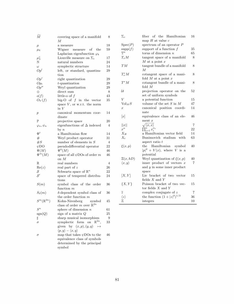
M covering space of a manifoldM

8

µ a measure 18µk Wigner measure of the

Laplacian eigenfunction ϕk

59

µcL Liouville measure on Σc 17N natural numbers 24ω symplectic structure 14

Opl left, or standard, quantiza-tion

29

Opr right quantization 29Opt t-quantization 29Opw Weyl quantization 29⊕ direct sum 8o(f) little-o of f 43OV (f) big-O of f in the vector

space V , or w.r.t. the normin V

35

p canonical momentum coor-dinate

14

P projective space 20ϕn, ψn eigenfunctions of ∆ indexed

by n4

Φt a Hamiltonian flow 14# Weyl product operator 31#S number of elements in S 4ψDO pseudodifferential operator 22Ψ(M) Ψ0(M) 46Ψm(M) space of all ψDOs of order m

on M46

R real numbers 4Re(z) real part of z 26S Schwartz space of Rn 22S ′ space of tempered distribu-

tions24

S(m) symbol class of the orderfunction m

36

Sδ(m) δ-dependent symbol class ofthe order function m

36

Sm(R2n) Kohn-Nirenberg symbolclass of order m over R2n

45

Sn sphere of dimension n 61sgn(Q) sign of a matrix Q 25] sharp musical isomorphism 9σ symplectic form on R2n,

given by (x, p), (y, q) 7→〈p, y〉 − 〈x, q〉

33

σ map that takes ψDOs to theequivalence class of symbolsdetermined by the principalsymbol

46

Σc fiber of the Hamiltonianmap H at value c

16

Spec(P ) spectrum of an operator Psupp(f) support of a function f 35Tn torus of dimension n 65TxM tangent space of a manifold

M at a point x8

TM tangent bundle of a manifoldM

8

T ∗xM cotangent space of a mani-fold M at a point x

8

T ∗M cotangent bundle of a mani-fold M

8

U projection operator on theset of uniform symbols

52

V a potential function 15VolMS volume of the set S in M 47x canonical position coordi-

nate14

[x] equivalence class of an ele-ment x

46

||x||√〈x, x〉 7

xα∏ni=1 x

αii 22

XH a Hamiltonian vector field 14Xt Bunimovich stadium with

aspect ratio t63

ξ(x, p) the Hamiltonian symbol|p|2 + V (x), where V is apotential

40

Ξ(x, hD) Weyl quantization of ξ(x, p) 40〈x, y〉 inner product of vectors x

and y in some inner productspace

7

[X,Y ] Lie bracket of two vectorfields X and Y

15

X,Y Poisson bracket of two vec-tor fields X and Y

15

z complex conjugate of z 7

〈z〉 the function (1 + |z|2)1/2 36Z integers 10

81

Appendix V: Index of Mathematical Objects and Figures

List of theorems and definitions, in temporal order

Definition 1.1.1 L2 space of functions 7Example 1.1.2 Riemannian metrics 8Definition 1.1.3 Laplace-Beltrami operator 9Proposition 1.1.4 Green’s second identity 10Theorem 1.1.5 spectral theorem and eigenfunction basis of ∆ 10Example 1.1.6 Laplacian on S1 10Example 1.1.7 Laplacian on a rectangular domain 11Example 1.1.8 Laplacian on D 11Example 1.2.1 circular and Sinai billiard flows 12Example 1.2.2 Newton’s second law 15Definition 1.2.3 integrability 15Theorem 1.2.4 Liouville-Arnold, [dS08] 16Example 1.2.5 integrability of two-dimensional systems 16Example 1.2.6 Hamiltonian nature of billiards 16Definition 1.2.7 Liouville measure 17Theorem 1.2.8 geodesic and cogeodesic flow, [Mil64] 17Example 1.2.9 geodesic integrability of surfaces of revolution, [Kiy00] 17Definition 1.2.10 ergodicity and mixing 18Theorem 1.2.11 weak ergodic theorem 18Theorem 1.2.12 ergodicity of geodesic flow on a negatively curved manifold, [Bal95] 19Definition 2.1.1 Schwartz space 22Definition 2.1.2 Fourier transform 22Proposition 2.1.3 Fourier transform of an exponential of a real quadratic form, [Zwo12] 23Theorem 2.1.4 properties of F 23Proposition 2.1.5 estimates of F 24Definition 2.1.6 tempered distributions 24Example 2.1.7 Heavyside step function 24Example 2.1.8 Fourier transform of Dirac delta 24Proposition 2.1.9 Fourier transform of an imaginary quadratic exponential, [Zwo12] 25Example 2.1.10 uncertainty principle in R, [Du09] 27Definition 2.1.11 semiclassical Fourier transform 27Theorem 2.1.12 useful properties of Fh 28Theorem 2.1.13 generalized uncertainty principle, [Mar02, Zwo12] 28Definition 2.1.14 symbols and quantization 29Example 2.1.15 quantizing a p-dependent symbol 29Example 2.1.16 quantizing an inner product 29Example 2.1.17 quantizing an x-dependent symbol, [Zwo12] 30Example 2.1.18 quantizing a linear symbol, [Mar02] 30Theorem 2.1.19 properties of quantization 30Theorem 2.1.20 relation of quantization to commutators, [GS12, Zwo12] 30Theorem 2.1.21 conjugation by the semiclassical Fourier transform 31Lemma 2.2.1 quantizing an exponential of a linear symbol, [Zwo12] 31Lemma 2.2.2 Fourier decomposition of Opw(a) 32Theorem 2.2.3 quantization composition theorem, [DS99] 33Lemma 2.2.4 quantizing exponentials of quadratic forms, [Zwo12] 34Theorem 2.2.5 integral representation formula for composed symbols 35Theorem 2.2.6 semiclassical expansion [Mar02, UW10, Zwo12] 35

82

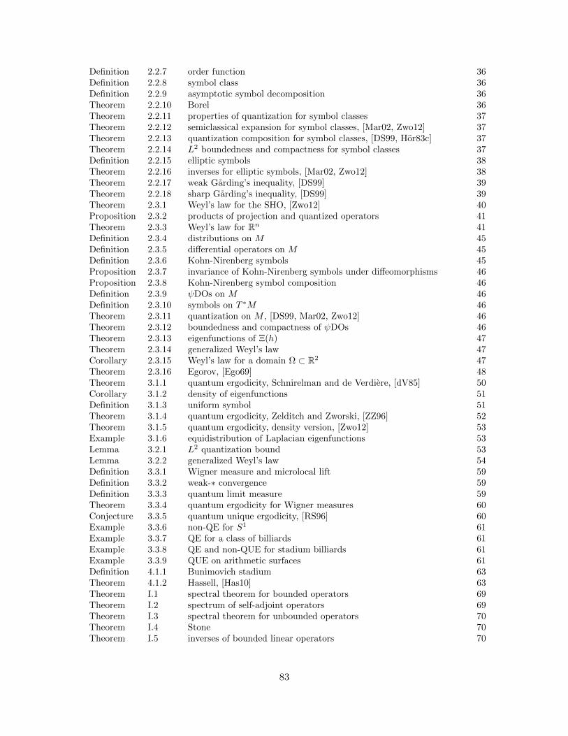
Definition 2.2.7 order function 36Definition 2.2.8 symbol class 36Definition 2.2.9 asymptotic symbol decomposition 36Theorem 2.2.10 Borel 36Theorem 2.2.11 properties of quantization for symbol classes 37Theorem 2.2.12 semiclassical expansion for symbol classes, [Mar02, Zwo12] 37Theorem 2.2.13 quantization composition for symbol classes, [DS99, Hor83c] 37Theorem 2.2.14 L2 boundedness and compactness for symbol classes 37Definition 2.2.15 elliptic symbols 38Theorem 2.2.16 inverses for elliptic symbols, [Mar02, Zwo12] 38Theorem 2.2.17 weak Garding’s inequality, [DS99] 39Theorem 2.2.18 sharp Garding’s inequality, [DS99] 39Theorem 2.3.1 Weyl’s law for the SHO, [Zwo12] 40Proposition 2.3.2 products of projection and quantized operators 41Theorem 2.3.3 Weyl’s law for Rn 41Definition 2.3.4 distributions on M 45Definition 2.3.5 differential operators on M 45Definition 2.3.6 Kohn-Nirenberg symbols 45Proposition 2.3.7 invariance of Kohn-Nirenberg symbols under diffeomorphisms 46Proposition 2.3.8 Kohn-Nirenberg symbol composition 46Definition 2.3.9 ψDOs on M 46Definition 2.3.10 symbols on T ∗M 46Theorem 2.3.11 quantization on M , [DS99, Mar02, Zwo12] 46Theorem 2.3.12 boundedness and compactness of ψDOs 46Theorem 2.3.13 eigenfunctions of Ξ(h) 47Theorem 2.3.14 generalized Weyl’s law 47Corollary 2.3.15 Weyl’s law for a domain Ω ⊂ R2 47Theorem 2.3.16 Egorov, [Ego69] 48Theorem 3.1.1 quantum ergodicity, Schnirelman and de Verdiere, [dV85] 50Corollary 3.1.2 density of eigenfunctions 51Definition 3.1.3 uniform symbol 51Theorem 3.1.4 quantum ergodicity, Zelditch and Zworski, [ZZ96] 52Theorem 3.1.5 quantum ergodicity, density version, [Zwo12] 53Example 3.1.6 equidistribution of Laplacian eigenfunctions 53Lemma 3.2.1 L2 quantization bound 53Lemma 3.2.2 generalized Weyl’s law 54Definition 3.3.1 Wigner measure and microlocal lift 59Definition 3.3.2 weak-∗ convergence 59Definition 3.3.3 quantum limit measure 59Theorem 3.3.4 quantum ergodicity for Wigner measures 60Conjecture 3.3.5 quantum unique ergodicity, [RS96] 60Example 3.3.6 non-QE for S1 61Example 3.3.7 QE for a class of billiards 61Example 3.3.8 QE and non-QUE for stadium billiards 61Example 3.3.9 QUE on arithmetic surfaces 61Definition 4.1.1 Bunimovich stadium 63Theorem 4.1.2 Hassell, [Has10] 63Theorem I.1 spectral theorem for bounded operators 69Theorem I.2 spectrum of self-adjoint operators 69Theorem I.3 spectral theorem for unbounded operators 70Theorem I.4 Stone 70Theorem I.5 inverses of bounded linear operators 70

83

Theorem I.6 Courant-Fischer 71Theorem I.7 estimates of N(λ) 71Lemma II.1 quadratic phase asymptotics, [Zwo12] 72Proposition II.2 stationary phase formula, [Zwo12] 73Figure 1.1 contour plots of Dirichlet Laplacian eigenfunctions 11Figure 1.2 trajectories on the circular and Sinai billiards 13Figure 1.3 billiard flow on different domains 13Figure 2.1 contours Ck used in the proof of Proposition 2.1.9 26Figure 3.1 scarring eigenfunctions on the Bunimovich stadium, [Kin13] 61Figure 4.1 trajectories on the Bunimovich stadium 64Table 1 a compilation of quantization procedures 72Table 2 a compilation of quantization examples 72Script 1 Dirichlet Laplacian eigenfunctions on a square 75Script 2 Dirichlet Laplacian eigenfunctions on a circle 75Script 3 rectangle billiard trajectories 76Script 4 circle billiard trajectories 76Script 5 Bunimovich billiard trajectories 77Script 6 Sinai billiard trajectories 78Script 7 Barnett billiard trajectories 78Script 8 triangle billiard trajectories 79

84

Index

L2 space, 7

billiards, 12Barnett stadium, 13, 66Bunimovich stadium, 5, 61, 63Sinai stadium, 12

distribution, 24on a manifold, 45tempered distribution, 24

Egorov’s theorem, 4, 48, 60correspondence principle, 4

eigenfunction, 4, 10, 47, 51eigenvalue, 4, 10, 47, 69

eigenvalue equation, 10spectrum, 7, 50, 69

ergodicity, 6, 18, 68Anosov property, 19Arnold’s cat map, 65Hopf theorem, 19weak ergodic theorem, 18

Fourier transform, 22Schwartz space, 22semiclassical Fourier transform, 27

geodesic flow, 17Garding’s inequality, 39

Hamiltonian formulation of mechanics, 14configuration space, 14Hamiltonian, 14Hamiltonian flow, 14Hamiltonian system, 15integrability, 15Liouville-Arnold theorem, 16phase space, 14

Hamiltonian operator, 40, 47, 51Hamiltonian symbol, 40, 51Hecke operator, 6Heisenberg uncertainty principle, 27, 28Helmholtz equation, 4

Laplace-Beltrami operator, 7, 51, 53, 68Dirichlet Laplacian, 10in local coordinates, 9Neumann Laplacian, 10

level set, 16Lie bracket, 15Liouville measure, 6, 16

microlocal lift, 59musical isomorphism, 8

Poisson bracket, 15, 48pseudodifferential operator, 29, 46

on a manifold, 46

quantization, 21, 29t-quantization, 29composition theorem, 33, 37left quantization, 29on a manifold, 46right quantization, 29Weyl quantization, 21, 29

quantum chaos, 4, 12, 68quantum ergodicity, 5

arithmetic quantum ergodicity, 62quantum ergodicity theorem, 5, 50, 60quantum limit measure, 59quantum unique ergodicity, 5, 50, 58, 60quantum unique ergodicity conjecture, 6, 60

Riemannian manifold, 6, 8local coordinates, 8metric tensor, 8

Schrodinger equation, 5self-adjoint operator, 20, 69semiclassical analysis, 21, 68

semiclassical expansion, 35, 37simple harmonic oscillator, 40spectral statistics, 66

Berry-Tabor conjecture, 67Bohigas-Giannoni-Schmidt conjecture, 67consecutive level spacing distribution, 66

spectral theorem, 10, 69symbol, 29

ellipticity, 38Kohn-Nirenberg class, 45on a manifold, 46order function, 36symbol class, 36uniformity, 51

symplectic geometry, 14

unitary flow, 20, 48

weak-∗ convergence, 51, 59Weyl product operator, 31Weyl’s law, 4, 12, 40

for Rn, 41for compact Riemannian manifolds, 47for Euclidean planar domains, 47for the simple harmonic oscillator, 40

Wigner measure, 20, 53, 59

85

References

[AN07] N. Anantharaman and S. Nonnenmacher. Half-delocalization of eigenfunctionsfor the Laplacian on an Anosov manifold. Ann. Inst. Fourier, 2007.

[Ana08] N. Anantharaman. Entropy and the localization of eigenfunctions. Ann. ofMath, 2(168):435–475, 2008.

[Ana09] N. Anantharaman. Chaotic vibrations and strong scars. News. Euro. Math.Soc., 74:19–24, 2009.

[Ana10] N. Anantharaman. Eigenfunctions of the Laplacian on negatively curved man-ifolds: a semiclassical approach. In Clay Mathematics Proceedings, volume 10,2010. Available online at http://www.math.u-bordeaux1.fr/~pthieull/

Recherche/KamFaible/Publications/Anantharaman2010_03.pdf.

[Ano67] D. V. Anosov. Geodesic flows on closed Riemannian manifolds of negative cur-vature. Trudy Mat. Inst. Steklov., 90, 1967.

[Arn78] V. I. Arnold. Mathematical Methods of Classical Mechanics. Springer, 1978.

[Bac07] A. Backer. Quantum chaos in billiards. Comp. in Sci. and Eng., 9(3):60–64,2007.

[Bal95] W. Ballman. Lectures on Spaces of Nonpositive Curvature. Birkhauser, 1995.

[Bar06] A. Barnett. Asymptotic rate of quantum ergodicity in chaotic Euclidean bil-liards. Comm. Pure Appl. Math., 59(10):1457–1488, 2006.

[Bar12] C. Bar. Renormalized integrals and a path integral formula for the heat kernelon a manifold. Preprints des Inst. fur Mathematik der Universitat Potsdam,21(1):1–18, 2012.

[Bar14] A. Barnett. Alex Barnett: publications, talks, notes, March 2014. http://www.math.dartmouth.edu/~ahb/pubs.html.

[BD11] P. H. Bezandry and T. Diagana. Almost Periodic Stochastic Processes. Springer,2011.

[Ber89] M. Berry. Quantum scars of classical closed orbits in phase space. Proc. Roy.Soc. London, 423:219–231, 1989.

[Ber03] M. Berry. Quantum chaology. Available online at http://www.phy.bris.ac.

uk/people/berry_mv/the_papers/berry358.pdf, 2003.

[BGS84] O. Bohigas, M. J. Giannoni, and C. Schmidt. Characterization of chaotic quan-tum spectra and universality of level fluctuation laws. Phys. Rev. Let., 52(1):1–4,1984.

[Bi01] S. De Bievre. Quantum chaos: a brief first visit. Con. Math., 289:161–218, 2001.

86

[Bi04] S. De Bievre. Quantum chaos: beyond the Schnirelman theorem.Available online at http://www-gat.univ-lille1.fr/~debievre/Talks/

texaslecture04sept.pdf, July 2004.

[BK10] P. Bourgade and J. P. Keating. Quantum chaos, random matrix theory, and theRiemann ζ-function. Seminaire Poincare XIV, pages 115–153, 2010.

[BL03] J. Bourgain and E. Linderstrauss. Entropy of quantum limits. Comm. Math.Phys., 233:153–171, 2003.

[Bro11] S. Brooks. Lecture notes — intro to quantum chaos. SUNY lecture notes.Available online at http://www.math.sunysb.edu/~sbrooks/qcNotesSp11.

pdf, 2011.

[BSS98] A. Backer, R. Schubert, and P. Stifter. Rate of quantum ergodicity in Euclideanbilliards. Phys. Rev. E, 57:5425, 1998.

[Bun79] L. Bunimovich. On the ergodic properties of nowhere dispersing billiards. Comm.Math. Phys., 65:295–312, 1979.

[BY13] P. Bourgade and H. T. Yau. The eigenvector moment flow and local quantumunique ergodicity. Preprint available online at http://www.math.harvard.edu/

~bourgade/papers/EMF.pdf, 2013.

[CCFI11] O. Calin, D. C. Chang, K. Furutani, and Chisato Iwasak. Heat Kernels for Ellip-tic and Sub-elliptic Operators: Methods and Techniques. Applied and NumericalHarmonic Analysis. Birkhauser, 2011.

[CH89] R. Courant and D. Hilbert. Methods of Mathematical Physics, volume 1. Wiley-VCH, 1989.

[Dav95] E. B. Davies. Spectral Theory and Differential Operators. Cambridge UP, 1995.

[dC94] M. do Carmo. Differential Forms and Applications. Springer, 1994.

[dMG81] L. Boutet de Monvel and V. Guillemin. The Spectral Theory of Operators, vol-ume 99. Ann. Math. Studies, 1981.

[DS99] M. Dimassi and J. Sjostrand. Spectral Asymptotics in the Semi-Classical Limit,volume 268 of Lecture Note Series. Cambridge UP, 1999.

[dS08] A. Cannas da Silva. Lectures on Symplectic Geometry, volume 1764 of LectureNotes in Mathematics. Springer, 2008.

[Du09] W. Du. Fourier analysis and the uncertainty principle. U. Chicago REU paper.Available online at http://www.math.uchicago.edu/~may/VIGRE/VIGRE2009/REUPapers/Du.pdf, 2009.

[Dui95] J. J. Duistermaat. Fourier Integral Operators, volume 130 of Progress in Math-ematics. Birkhauser, 1995.

87

[dV77] Y. Colin de Verdiere. Quasi-modes sur les varietes Riemanniennes. Invent. Math,3:15–52, 1977.

[dV85] Y. Colin de Verdiere. Ergodicite et fonctions propres du Laplacien. Comm.Math. Phys., 102:497–502, 1985.

[dV08] Y. Colin de Verdiere. Semi-classical measures and entropy. Vol 2006/2007.Seminare Bourbaki, Asterisque No. 317:393–414, 2008.

[Ego69] Y. Egorov. The canonical transformations of a pseudo-differential operator.Uspehi. Mat. Nauk., 24:235–236, 1969.

[ER05] A. Edelman and N. R. Rao. Random matrix theory. Acta Numerica, pages 1–65,2005.

[Eva98] L. Evans. Partial Differential Equations, volume 19 of Graduate Studies inMathematics. AMS, 1998.

[FN04] F. Faure and S. Nonnenmacher. On the maximal scarring for quantum cat mapeigenstates. Comm. Math. Phys., 245:201–214, 2004.

[FNdB03] F. Faure, S. Nonnenmacher, and S. de Bievre. Scarred eigenstates for quantumcat maps of minimal periods. Comm. Math. Phys., 239:449–492, 2003.

[GL93] P. Gerard and E. Leichtman. Ergodic properties of eigenfunctions for the Dirich-let problem. Duke Math. Journal, 71:559–607, 1993.

[Gri95] D. J. Griffiths. Introduction to Quantum Mechanics. Prentice Hall, 1995.

[GS06] V. A. Galaktionov and S. R. Svirshchevskii. Exact Solutions and InvariantSubspaces of Nonlinear Partial Differential Equations in Mechanics and Physics.CRC Applied Mathematics and Nonlinear Science. Chapman and Hall, 2006.

[GS12] V. Guillemin and S. Sternberg. Semi-classical analysis. Harvard lecturenotes. Available online at http://www.math.harvard.edu/~shlomo/docs/

Semi_Classical_Analysis_Start.pdf, 2012.

[Gut90] M. C. Gutzwiller. Chaos in Classical and Quantum Mechanics, volume 1 ofInterdisciplinary Applied Mathematics. Springer, 1990.

[Gut09] B. Gutkin. Note on converse quantum ergodicity. Proc. Amer. Math. Soc.,137(8):2795–2800, 2009.

[GWW92] C. Gordon, D. L. Webb, and S. Wolpert. One cannot hear the shape of a drum.Bull. Amer. Math. Soc., 27:134–138, 1992.

[Has10] A. Hassell. Ergodic billiards that are not quantum unique ergodic. Ann. Math.,171(1):605–618, January 2010.

[Has11] A. Hassell. What is quantum unique ergodicity? Aus. Math. Soc. Gazette,38:158–167, July 2011.

88

[Has12] A. Hassell. ESI lectures on semiclassical analysis and quantum er-godicity 2012. Available online at http://ipht.cea.fr/Pisp/stephane.

nonnenmacher/ESI2012/Hassell-semiclassical-analysis3.pdf, 2012.

[Hel84] E. J. Heller. Bound-state eigenfunctions of classically chaotic Hamiltoniansysyems: scars of periodic orbits. Phys. Rev. Lett., 53(16):1515–1518, 1984.

[Hel88] B. Helffer. Semi-Classical Analysis for the Schrdinger Operator and Applications,volume 1336 of Lecture Notes in Mathematics. Springer, 1988.

[Hel10] B. Helffer. Spectral theory and applications. an elementary introductory course.bucarest version 2010. Available online at http://www.math.u-psud.fr/

~helffer/m2bucarest2010.pdf, 2010.

[HMR87] B. Helffer, A. Martinez, and D. Robert. Ergodicite et limite semi-classique.Comm. Math. Phys., 109(2):177–352, 1987.

[HO88] E. J. Heller and P. W. O’Connor. Quantum localization for a strongly classicalchaotic system. Phys. Rev. Lett., 61(20):2288–2291, 1988.

[Hor83a] L. Hormander. The Analysis of Linear Partial Differential Operators I: Dis-tribution Theory and Fourier Analysis. A Series of Comprehensive Studies inMathematics. Springer-Verlag, 1983.

[Hor83b] L. Hormander. The Analysis of Linear Partial Differential Operators II: Differ-ential Operators with Constant Coefficients, volume 257 of A Series of Compre-hensive Studies in Mathematics. Springer-Verlag, 1983.

[Hor83c] L. Hormander. The Analysis of Linear Partial Differential Operators III:Pseudo-Differential Operators, volume 257 of A Series of Comprehensive Studiesin Mathematics. Springer-Verlag, 1983.

[Hor83d] L. Hormander. The Analysis of Linear Partial Differential Operators IV: FourierIntegral Operators, volume 257 of A Series of Comprehensive Studies in Mathe-matics. Springer-Verlag, 1983.

[Hov51] L. Van Hove. Sur le probleme des relations entre les transformations unitairesde la mecanique quantique et les transformations canoniques de la mecaniquesclassique. Acad. Roy. Belgique. Bull. Cl. Sci., 5(37):610–620, 1951.

[HS10] R. Holowinsky and K. Soundararajan. Mass equidistribution for Hecke eigen-forms. Ann. Math., 172(2):1517–1528, 2010.

[HZ04] A. Hassell and S. Zelditch. Quantum ergodicity of boundary values of eigenfunc-tions. Comm. Math. Phys., 248(1):119–168, 2004.

[Jak10] D. Jakobson. Spectral theory, geometry and dynamical systems. Available onlineat http://www.math.mcgill.ca/jakobson/papers/winter10.pdf, 2010.

[Jos11] J. Jost. Riemannian Geometry and Geometric Analysis. Universitext. Springer,2011.

89

[Kac66] M. Kac. Can one hear the shape of a drum? Amer. Math. Monthly, 73(4):1–23,1966.

[Kin13] C. King. Exploring quantum, classical and semiclassical chaos in the stadiumbilliard, July 2013. http://www.dhushara.com/DarkHeart/QStad/QStad.htm.

[Kiy00] K. Kiyohara. On manifolds whose geodesic flows are integrable. Suuri kaisekikenkyuujo koukyuu roku (RIMS), 1150:162–164, 2000.

[Kow09] E. Kowalski. Spectral theory in hilbert spaces. Available online at http://www.math.ethz.ch/~kowalski/spectral-theory.pdf, 2009.

[KZ02] H. J. Korsch and F. Zimmer. Chaotic billiards. In K. H. Hoffman andM. Schreiber, editors, Computational Statistical Physics: From Billards toMonte-Carlo, chapter 2, pages 15–37. Springer, 2002.

[Lan98] N. P. Landsman. Mathematical Topics Between Classical and Quantum Mechan-ics. Springer Monograph in Mathematics. Springer, 1998.

[Lee09] J. M. Lee. Manifolds and Differential Geometry, volume 107 of Graduate Studiesin Mathematics. AMS, 2009.

[Lin01] E. Lindenstrauss. On quantum unique ergodicity for Γ\H×H. Internat. Math.Res. Notices, pages 913–933, 2001.

[Lin06] E. Lindenstrauss. Invariant measures and arithmetic quantum unique ergodicity.Ann. Math., 163(1):165–219, 2006.

[LS95] W. Luo and P. Sarnak. Quantum ergodicity of eigenfunctions on PSL2(Z)\H2.IHES Publ., 81:207–237, 1995.

[LS04] W. Luo and P. Sarnak. Quantum variance for Hecke eigenforms. Annales Scient.de I’Ecole Norm. Sup., 37:769–799, 2004.

[Mar02] A. Martinez. An Introduction to Semiclassical and Microlocal Analysis. Univer-sitext. Springer, 2002.

[Mar06] J. Marklof. Arithmetic quantum chaos. Encyc. Math. Phys., 1:212–220, 2006.

[Mil64] J. Milnor. Eigenvalues of the Laplace operator on certain manifolds. PNAS,51(4):542, 1964.

[Mil00] A. Miller. Riemannian manifolds with integrable geodesic flows. Available onlineat http://math.berkeley.edu/~alanw/240papers00/miller.pdf, 2000.

[MR00] J. Marklof and Z. Rudnick. Quantum unique ergodicity for parabolic maps. Geo.and Func. Anal., 10:1554–1578, 2000.

[MU08] R. B. Melrose and G. Uhlman. An introduction to microlocal analysis. MITlecture notes. Available online at http://www-math.mit.edu/~rbm/books/

imaast.pdf, 2008.

90

[Non10] S. Nonnenmacher. Anatomy of quantum chaotic eigenstates. Seminaire PoincareXIV, pages 1–43, 2010.

[Pet07] M. Pettini. Geometry and Topology in Hamiltonian Dynamics and StatisticalMechanics, volume 33 of Interdisciplinary Applied Mathematics. Springer, 2007.

[RC01] D. N. Ghosh Roy and L. S. Couchman. Inverse Problems and Inverse Scatteringof Plane Waves. Academic Press, 2001.

[Ros97] S. Rosenberg. The Laplacian on a Riemannian Manifold, volume 31 of LondonMathematical Society Student Texts. Cambridge UP, 1997.

[RS80] M. Reed and B. Simon. Methods of Modern Mathematical Physics I: FunctionalAnalysis. Academic Press, 1980.

[RS96] Z. Rudnick and P. Sarnak. The behaviour of eigenstates of arithmetic hyperbolicmanifolds. Comm. Math. Phys., 161(1):195–213, 1996.

[RS12] G. Rudolph and M. Schmidt. Differential Geometry and Mathematical Physics:Part I. Manifolds, Lie Groups and Hamiltonian Systems. Theoretical and Math-ematical Physics. Springer, 2012.

[Rud08] Z. Rudnick. What is... quantum chaos? Notices of the AMS, 55(1):32–34, 2008.

[Sak93] J. J. Sakurai. Modern Quantum Mechanics. Addison Wesley, 1993.

[Sar03] P. Sarnak. Spectra of arithmetic manifolds. BAMS, 40:441–478, 2003.

[Sar11] P. Sarnak. Recent progress on the quantum unique ergodicity conjecture. Bull.Amer. Math. Soc., 48(2):221–228, 2011.

[Sch74] A. I. Schnirelman. Ergodic properties of eigenfunctions. Usp. Math. Nauk.,29(6):181–182, 1974.

[Sha94] R. Shankar. Principles of Quantum Mechanics. Plenum Press, 1994.

[Sie10] M. Sieber. Quantum billiards. Postgraduate research conference:Mathematical billiard and their applications. Available online athttp://www.maths.bris.ac.uk/~macpd/bristol10/Mathematical%

20Billiards%20and%20thewir%20Applications/QBilliards.pdf, 2010.

[Sin70] Y. G. Sinai. Dynamical systems with elastic reflections. Usp. Math. Nauk.,25:137–189, 1970.

[Sou10] K. Soundararajan. Quantum unique ergodicity for SL2(z)/h. Ann. Math.,172(2):1529–1538, 2010.

[SS03] E. M. Stein and R. Shakarchi. Complex Analysis, volume 2 of Princeton Lecturesin Analysis. Princeton UP, 2003.

[SS11] E. M. Stein and R. Shakarchi. Functional Analysis: Introduction to FurtherTopics in Analysis, volume 4 of Princeton Lectures in Analysis. Princeton UP,2011.

91

[Sta13] TEX StackExchange. Chaotic billiard with tikz, December 2013. http://tex.

stackexchange.com/questions/149741/chaotic-billiard-with-tikz.

[Ste10] S. Sternberg. Dynamical Systems. Dover, 2010.

[Str83] R. S. Strichartz. Analysis of the Laplacian on the complete Riemannian manifold.J. Functional Anal., 52:48–79, 1983.

[SVM07] J. A. Sanders, F. Verhulst, and J. Murdock. Averaging Methods in NonlinearDynamical Systems, volume 59 of Applied Mathematical Sciences. Springer,2007.

[Tao07] T. Tao. Simons lecture I: Structure and randomness in Fourier analysis andnumber theory, April 2007. http://terrytao.wordpress.com/2007/04/05/

simons-lecture-i-structure-and-randomness-in-fourier-analysis-and

-number-theory/.

[Tao08] T. Tao. Hassell’s proof of scarring for the Bunimovich stadium, July 2008. http://terrytao.wordpress.com/2008/07/07/hassells-proof-of-scarring

-for-the-bunimovich-stadium/.

[Tao09] T. Tao. Fourier transform. Preprint available online at http://www.math.ucla.edu/~tao/preprints/fourier.pdf, 2009.

[Tau11] C. H. Taubes. Differential Geometry: Bundles, Connections, Metrics and Cur-vature, volume 23 of Graduate Texts in Mathematics. Oxford UP, 2011.

[UW10] A. Uribe and Z. Wang. A brief introduction to semiclassical analysis. U.Mich. mini-course notes. Available online at http://www-personal.umich.

edu/~wangzuoq/papers/minicourse_Dart.pdf, 2010.

[Wey16] H. Weyl. Uber die Gleichverteilung von Zahlen mod. Eins. Math. Ann.,77(3):313–352, 1916.

[Yau82] S. T. Yau. Survey on partial differential equations in differential geometry. Ann.Math. Stud., 102:3–71, 1982.

[Zel87] S. Zelditch. Uniform distribution of eigenfunctions on compact hyperbolic sur-faces. Duke Math. Journal, 55:919–941, 1987.

[Zel92] S. Zelditch. Quantum ergodicity on the sphere. Comm. Math. Phys., 146:61–71,1992.

[Zel10] S. Zelditch. Recent developments in mathematical quantum chaos. Cur. Dev.Math., 2009:1–204, 2010.

[Zwo12] M. Zworski. Semiclassical Analysis, volume 138 of Graduate Studies in Mathe-matics. AMS, 2012.

[ZZ96] S. Zelditch and M. Zworski. Ergodicity of eigenfunctions for ergodic billiards.Comm. Math. Phys., 175(3):673–682, 1996.

92