quantum mechanics of collision processes ( 1)
TRANSCRIPT

“Quantenmechanik der Stoßvorgänge,” Zeit. Phys. 38 (1927), 803-827.
Quantum mechanics of collision processes (1).
By Max Born in Göttingen.
(Received on 21 July 1926)
Translated by D. H. Delphenich
The Schrödinger form of quantum mechanics allows one to define the frequency of a state in a natural way with the help of the intensity of the associated eigen-vibration. This viewpoint leads to a theory of collision processes in which the transition probabilities are determined by the asymptotic behavior of aperiodic solutions. Introduction. Collision processes not only yield the most convincing experimental proof of the basic assumptions of quantum theory, but also seem suitable for explaining the physical meaning of the formal laws of the so-called “quantum mechanics.” Indeed, as it seems, it always produces the correct term values of the stationary states and the correct amplitudes for the oscillations that are radiated by the transitions, but opinions are divided regarding the physical interpretation of the formulas. The matrix form of quantum mechanics (2) that was founded by Heisenberg and developed by him and the author of this article starts from the thought that an exact representation of processes in space and time is quite impossible and that one must then content oneself with presenting the relations between the observed quantities, which can only be interpreted as properties of the motions in the limiting classical cases. On the other hand, Schrödinger (3) seems to have ascribed a reality of the same kind that light waves possessed to the waves that he regards as the carriers of atomic processes by using the de Broglie procedure; he attempts “to construct wave packets that have relatively small dimensions in all directions,” and which can obviously represent the moving corpuscle directly. Neither of these viewpoints seems satisfactory to me. Here, I would like to try to give a third interpretation and probe its utility in collision processes. I shall recall a remark that Einstein made about the behavior of the wave field and light quanta. He said that perhaps the waves only have to be wherever one needs to know the path of the corpuscular light quanta, and in that sense, he spoke of a “ghost field.” It determines the probability that a light quantum − viz., the carrier of energy and impulse – follows a certain path; however, the field itself is ascribed no energy and no impulse.
(1) A preliminary announcement appeared in Zeit. Phys. 37 (1926), 863. (2) W. Heisenberg, Zeit. Phys. 33 (1925), 879; M. Born and P. Jordan, ibidem 34 (1925), 858; M. Born, W. Heisenberg, and P. Jordan, ibidem 35 (1926), 557. See also P. A. M. Dirac, Proc. Roy. Soc. 109 (1925), 642; 110 (1926), 561. (3) E. Schrödinger, Ann. d. Phys. 79 (1926), 361, 489, 734. Cf., the second paper, pp. 499. Furthermore, Naturw. 14 (1926), 664.

Born – Quantum mechanics of collision processes. 2
One would do better to postpone these thoughts, when coupled directly to quantum mechanics, until the place of the electromagnetic field in the formalism has been established. However, from the complete analogy between light quanta and electrons, one might consider formulating the laws of electron motion in a similar manner. This is closely related to regarding the de Broglie-Schrödinger waves as “ghost fields,” or better yet, “guiding fields.” I would then like to pursue the following idea heuristically: The guiding field, which is represented by a scalar function ψ of the coordinates of all particles that are involved and time, propagates according to Schrödinger’s differential equation. However, impulse and energy will be carried along as when corpuscles (i.e., electrons) are actually flying around. The paths of these corpuscles are determined only to the extent that they are constrained by the law of energy and impulse; moreover, only a probability that a certain path will be followed will be determined by the function ψ. One can perhaps summarize this, somewhat paradoxically, as: The motion of the particle follows the laws of probability, but the probability itself propagates in accord with causal laws (1). If one surveys the three levels in the development of quantum theory then one will see that the lowest one – viz., that of periodic processes – is entirely unsuitable for testing the utility of such a conception. The second level − namely, the level of aperiodic, stationary processes − achieves somewhat more; we would like to concern ourselves with it in the present paper. However, the third level – viz., that of non-stationary evolution – can actually be decisive; there, one must show whether the interference of damped “probability waves” suffices to explain the phenomena that apparently point to a coupling that does not relate to space-time. Making this concept precise is possible only on the basis of some further mathematical development (2); therefore, we shall turn to that directly, so that we can then return to the hypothesis itself later on. § 1. Definition of the weights and frequencies for periodic systems. We begin with an entirely formal consideration of the discrete, stationary states of a non-degenerate system. They can be characterized by Schrödinger’s differential equation:
[H – W, ψ] = 0. (1) Let the eigenfunctions be normalized to 1 (3):
( ) ( )n mq q dqψ ψ ∗∫ = δmn . (2)
Any arbitrary function ψ(q) can be developed in eigenfunctions:
(1) That means that the knowledge of the state at all points at a moment will establish the distribution of states at all later times. (2) N. Wiener of Cambridge, Mass. has graciously helped me with the mathematical details of this paper; I would like to express my thanks to him for that and acknowledge that I would not have reached my goal without him. (3) For the sake of simplicity, I shall set the density function equal to 1 here.

Born – Quantum mechanics of collision processes. 3
ψ(q) = ( )n nn
c qψ∑ . (3)
Up to now, all of the attention has been focused upon the eigenvibrations ψn and the eigenvalues Wn . The picture that we suggested in the introduction is closely related to the idea of connecting the superposition of functions that is represented in (3) with the probability that the state will appear with a certain frequency in a cloud of identical, uncoupled atoms. The completeness relation:
2| ( ) |q dqψ∫ = 2| |nn
c∑ (4)
leads to the idea that this integral can be regarded as the number of atoms. It then has the value 1 for the appearance of a single, normalized eigenvibration (or: the a priori weight of the state is 1), | cn |
2 means the frequency of the state n, and the total numbers can be combined additively from these components. In order to justify this interpretation, we shall consider, say, the motion of a massive point in three-dimensional space under the action of the potential energy U(x, y, z); the differential equation (1) will then read:
∆ψ + 2
2
8
h
π µ(W – U) ψ = 0. (5)
If one sets W, ψ in this equal to an eigenvalue Wn and an eigenfunction ψn, resp., multiplies the equation by nψ ∗ , and integrates over all space (dS = dx dy dz) then one will
obtain: 2
2
8( )m n n n mW U
h
π µψ ψ ψ ψ∗ ∗ ∆ + −
∫∫∫ dS = 0.
From Green’s theorem, and recalling the orthogonality conditions (2), that will give:
δmn Wn = 2
2 (grad grad )8 n m n m
hUψ ψ ψ ψ
π µ∗ ∗
⋅ +
∫∫∫ dS . (6)
Each energy level can then be regarded as the spatial integral of the energy density of the eigenvibrations. If one now defines the corresponding integral for any function:
W = 2
2 22 | grad | | |
8 n n
hUψ ψ
π µ
+
∫∫∫ dS (7)
then if one substitutes the development (3), one will get the expression for this:

Born – Quantum mechanics of collision processes. 4
W = 2| |n nn
c W∑ . (8)
According to our interpretation of the | cn |
2, the right-hand side is the total energy of a system of atoms; this mean value can then be represented as the spatial integral of the energy density of the function ψ. However, nothing will point to our Ansatz in favor of the others as long as we remain within the scope of periodic processes. § 2. Aperiodic systems. We now go on to the aperiodic processes and, for the sake of simplicity, we shall first consider the case of uniform, rectilinear motion along the x-axis. In that case, the differential equation reads:
2
2
d
dx
ψ + k2 ψ = 0, k2 =
2
2
8
h
π µW ; (1)
it has all positive values W for its eigenvalues and the eigenfunctions: ψ = c e± i k x.
In order to be able to define the weights and frequencies, one must, above all, normalize the eigenfunctions. The integral formula that is analogous to (2) breaks down (i.e., the integral is divergent); that is why one employs the “mean value” instead of it:
21lim | ( , ) |
2
a
aak x dx
aψ
+
−→∞ ∫ = 2
lim2
a ikx ikx
aa
ce e dx
a
+ −
−→∞ ∫ = 1; (2)
it follows from this that c = 1, and one has the normalized eigenfunctions:
ψ(k, x) = e± i k x. (3) Any function of x can be composed of these. In order to do that, one must choose the unit for the k-scale – i.e., one must establish which segments shall have the weight 1. For that, one considers the free motion to be a limiting case of a periodic one, namely, the eigenvibration of a finite piece of the x-axis. One then knows that the number per unit
length and per interval (k, k + dk) is equal to 2
k
π∆
= 1
λ ∆
, where λ is the wave length.
One will then set:
ψ(x) = ( ) ( , )2
kc k k x dψ
π+∞
−∞∫ = ( ) ikxc k e dk+∞
−∞∫ , (4)
with c(− k) = c* (k) (5)

Born – Quantum mechanics of collision processes. 5
and expect that | c(k) |2 will then be the measure of the frequency for the interval 1
2π dk.
For a mixture of atoms for which the eigenfunctions appear in the distribution that is given by c(k), let the number that is analogous to § 1, (4) be represented by the integral:
2| ( ) |x dxψ+∞
−∞∫ = 2
2
1( )
(2 )ikxdx c k e dk
π+∞ +∞
−∞ −∞∫ ∫ . (6)
If we take the case in which only the small interval k1 ≤ k ≤ k2 is occupied then:
( ) ikxc k e dk+∞
−∞∫ = 2
1
kikx
kc e dk∫ = 2 1( )ik x ik xc
e eix
− ,
in which c is a mean value. One will then have:
2| ( ) |x dxψ+∞
−∞∫ = 2 1 2 1
2
2 2
| |( )( )
4ik x ik x ik x ik xc dx
e e e exπ
+∞ − −
−∞− −∫
= 2
2 2 12 2
| |4 sin
4 2
k kc dx
xπ+∞
−∞
−∫ = 21
| |2
cπ
(k2 – k1).
Now, according to de Broglie, the impulse of the translatory motion that belongs to the eigenfunction (8) is equal to:
p = h
λ =
2
h
πk. (7)
It is, perhaps, not superfluous to remark that one can also formulate this as a “matrix”; one must then define the matrices in the continuous spectrum here, not by integrals, but by mean values:
p(k, k′) = 1 ( , )
lim ( , )2 2
a
aa
h k xk x dx
i a x
ψψπ
+ ∗
−→∞
′∂∂∫
= 1
lim2 2
aikx ik x
aa
he ik e dx
i aπ+ ′−
−→∞′∫ .
p(k, k′) = for ,
20 " .
hk k k
k kπ
′= ′≠
(8)
If one now replaces ∆k = k2 – k1 with 2
h
π ∆p then one will finally have:

Born – Quantum mechanics of collision processes. 6
2| ( ) |x dxψ+∞
−∞∫ = 2| |p
ch
∆. (9)
One then has the result that a cell of length ∆x = 1 and impulse extension ∆p = h will have weight 1, in agreement with the Ansatz of Sackur and Tetrode (1), which has been confirmed many times by experiments, and that | c(k) |2 is the frequency for a motion with
the impulse p = 2
h
πk.
We now go onto accelerated motion. Here, one can naturally define a certain distribution of processes in an analogous way. However, that is not a rational question to pose for collision processes. For those processes, any motion will have a rectilinear asymptote before and after the collision. The particle is then found to be in a practically free state for a very long time (in comparison to the actual duration of the collision) before and after the collision. In agreement with the experimental statement of the problem, one thus comes to the following viewpoint: Let the distribution function | c(k) |2 for the asymptotic motion be known before the collision; can one calculate the distribution function after the collision from it? Naturally, we are speaking only of a stationary particle current here. Mathematically, the problem then comes down to the following one: The stationary vibration field ψ must be distributed into ingoing and outgoing waves; they are asymptotically plane waves. One then represents both of them by means of a Fourier integral of the form (4) and chooses the coefficient function c(k) for the ingoing waves arbitrarily; it shall then shown that the c(k) is determined completely for the outgoing waves. It yields the distribution into which a prescribed particle mixture will be converted after the collision. In order to see the relationship clearly, we first treat the one-dimensional case. § 3. The asymptotic behavior of the eigenfunctions in a continuous spectrum with one degree of freedom. Schrödinger’s differential equation reads:
2 2
2 2
8d
dx h
ψ π µ+ (W – U(x)) ψ = 0, (1)
in which U(x) means the potential energy. To abbreviate, we set:
2
2
8
h
π µW = k2,
2
2
8
h
π µ U(x) = V(x); (2)
we will then have: 2
2
d
dx
ψ+ k2ψ = V ψ. (3)
(1) A. Sackur, Ann. d. Phys. 36 (1911), 958; 40 (1913), 67; H. Tetrode, Phys. Zeit. 14 (1913), 212; Ann. d. Phys. 38 (1912), 434.

Born – Quantum mechanics of collision processes. 7
We examine the asymptotic behavior of the solution at infinity. In order to get a simple relationship, we assume that V(x) vanishes faster than x−2 at infinity; i.e.:
| V(x) | < 2
K
x, (4)
in which K is a positive number (1). We now determine ψ(x) by a process of iteration; let:
u0(x) = eikx, (5) and let u1(x), u2(x), … be the solutions of the successive approximations:
2
2nd u
dx + k2 un = V un−1 ,
which vanishes as x → + ∞. One then has:
un(x) = 1
1( ) ( )sin ( )nx
u V k x dk
ξ ξ ξ ξ∞
− −∫ ,
as one can verify directly. One has:
| un(x) | ≤ 1
1| ( ) | | ( ) |nxu V d
kξ ξ ξ
∞
− ⋅∫ .
We now show that:
| un(x) | ≤ 1
!
nK
n kx
.
This is correct for n = 0, since it follows from (5) that | u0(x) | ≤ 1. We now assume that is it correct for n – 1:
| un−1(ξ) | ≤ 1
1
( 1)!
nK
n kξ
− −
;
it then follows that:
| un(x) | ≤ 1
1 21 1
( 1)!
nn
x
KK d
k n kξ ξ ξ
−∞ − + ⋅ − ∫ =
1
!
nK
n kx
,
as was asserted. As a result, the series:
ψ(x) = 0
( )nn
u x∞
=∑ (6)
(1) The cases of a pure Coulomb field and a dipole field are excluded by this assumption.

Born – Quantum mechanics of collision processes. 8
converges uniformly for every finite interval; it can then be differentiated term-wise arbitrarily often, and is then, as is easy to see, the desired solution to our differential equation. However, since all u1, u2, … vanish as x → + ∞, the function ψ will be asymptotic to u0 = eikx at positive infinity. In precisely the same way, one shows that there is a solution that is asymptotic to e−ikx as x → + ∞. Since the general solution has only two constants, it must asymptotically have the form:
ψ+(x) = a eikx + b e−ikx (7) as x → + ∞. Here, the degeneracy of the system makes its appearance; every energy value W is associated with two values k, − k and two linearly-independent solutions. In an entirely similar way, it follows that the general solution must have the same form as x → − ∞:
ψ −(x) = A eikx + B e−ikx. (8) In this, the amplitudes A, B are well-defined functions of a, b. We now decompose the solution into incoming and outgoing waves; for that, we add
the time factor eikυt 2
2k v Wh
πυ π = =
and set:
, ,
, .
e a
a e
i t i te a
i t i ta e
a c e A C e
b c e B C e
ϕ
ϕ
Φ
− − Φ
= == =
(9)
One will then have: ( ) ( )
( ) ( )
( ) ,
( ) .
e a
a e
ik x t ik x te a
ik x t ik x ta e
x c e c e
x C e C e
υ ϕ υ ϕ
υ υ
ψψ
+ + − − ++
+ +Φ − − +Φ−
= += +
(10)
The real parts of the terms that are denoted with the index e represent the incoming waves, while the terms that are denoted with an a represent the outgoing waves. We are interested in the case in which only one wave is incoming at x = + ∞. One will then have Ce = 0, and one can arbitrarily set ϕe = 0, moreover. One will then have:
( )( )
( )
( ) ,
( ) .
a
a
ik x tik x te a
ik x ta
x c e c e
x C e
υ ϕυ
υ
ψψ
− − ++ +
+ +Φ−
= +=
(11)
We have shown that ψ −(x) is determined in terms of ψ +(x) by integration; i.e., A, B are well-defined functions of a, b. In our case Ce = 0, so we will have B = 0, and one thus has two equations of the form:
( , ),
0 ( , ).
A A a b
B a b
= =
(12)

Born – Quantum mechanics of collision processes. 9
One can express b in terms of a using the second one, and one will then get A expressed in terms of a from the first one. However, that means that the constants of the reflected wave and the constants of the transmitted wave can be calculated from the amplitude of the incoming wave. One can now show that a relation exists between the intensities of the three waves. One obtains it most simply with the help of the energy theorem. § 4. The theorem of the conservation of energy. In order to derive this theorem, we return to the form of Schrödinger’s differential equation for which the assumption of vibrations that are purely periodic in time is still not made, so one will have a wave equation of the form:
2 2
2 2 2
1
x t
ψ ψυ
∂ ∂−∂ ∂
= 0. (1)
In this, υ is the wave velocity. One comes to Schrödinger’s equation when one, with de Broglie, sets (1):
hv = W = 2
2u U
µ + , υ = λv, h
λ = p = µ u;
one will then have:
2
1
υ =
2
2 2 2
1h
h vλ =
2 2
2
u
W
µ =
2
2
22
u
W
µ µ⋅,
2
1
υ =
2
2
W
µ (W – U). (2)
If one now seeks solutions whose time dependency is given by the factor e2πiυt = 2 i
Wtheπ
then one will get:
2 2
2 2
8d
dx h
ψ π µ+ (W – U) ψ = 0.
However, we now fix our attention on the general formula (1) and multiply the equation by ∂ψ / ∂t. One now has:
2
2x t
ψ ψ∂ ∂∂ ∂
= 2
x x t x x t
ψ ψ ψ ψ∂ ∂ ∂ ∂ ∂ − ∂ ∂ ∂ ∂ ∂ ∂
(1) We neglect relativity and calculate with classical mechanics.

Born – Quantum mechanics of collision processes. 10
= 2
1
2x x t t x
ψ ψ ψ∂ ∂ ∂ ∂ ∂ − ∂ ∂ ∂ ∂ ∂ .
If υ depends upon only v then we will get:
2 2
2
1 1
2 2x x t t x t
ψ ψ ψ ψυ
∂ ∂ ∂ ∂ ∂ ∂ − + ∂ ∂ ∂ ∂ ∂ ∂ = 0. (3)
If one integrates over all space then one will get:
2 2
2
1 1
2x t t x t
ψ ψ ψ ψυ
+∞+∞
−∞−∞
∂ ∂ ∂ ∂ ∂ − + ∂ ∂ ∂ ∂ ∂ ∫ dx = 0. (4)
As was pointed out in § 1, the space integral in this is to be interpreted as the total energy that is present in space. However, its expression does not interest us, since for us it will enter into the in-streaming and out-streaming energy, which will be represented by limiting terms. The time mean of the two terms vanishes for a temporally periodic process, and, with the use of the notations that were introduced in § 3, (7), (8), one will get:
x t
ψ ψ− −∂ ∂−∂ ∂
= x t
ψ ψ+ +∂ ∂−∂ ∂
. (5)
This equation states that the in-streaming energy is equal to the out-streaming energy. When we substitute the real part of the expression § 3, (10) in this, we will get:
2 2a eC C− = 2 2
a ec c− , (6)
or, in the case Ce = 0 [as in equation (11), § 3]:
2ec = 2 2
a ac C+ . (7)
However, that means that for any elementary wave of given k, the incoming intensity will be split into the intensities of the two waves that scatter to the right and left, or, in the language of the corpuscular theory: If a particle with a given energy enters the atom then it will either be reflected or it will continue on. The sum of the probabilities in these two outcomes is 1. The theorem of the conservation of energy then has the conservation of particle number as a consequence. The basis for that lies in the degeneracy of the system; any energy value belongs to several motions, and they will be related to each other.

Born – Quantum mechanics of collision processes. 11
§ 5. Generalization to three degrees of freedom. The inertial motion. We now consider a particle that moves in space under the action of the potential energy U(x, y, z). One then has the differential equation:
∆ψ − 2
2 2
1
t
ψυ
∂∂
= 0, (1)
which is analogous to (1), in which υ is once more given in the approximation of classical mechanics by (2), § 4. Here, the conservation law reads:
div 2
22
1 1grad (grad )
2t t t
ψ ψψ ψυ
∂ ∂ ∂ − + ∂ ∂ ∂ = 0, (2)
or, when integrated over space:
22
2
1 1(grad )
2d dS
t t t t
ψ ψ ψσ ψυ∞
∂ ∂ ∂ ∂ − + ∂ ∂ ∂ ∂ ∫ ∫ = 0, (3)
in which dS = dx dy dz, and dσ is the element of an infinitely-distant, closed surface with exterior normal v. For temporally periodic processes, it then follows from this that the temporal mean will be:
dt t
ψ ψ σ∞
∂ ∂∂ ∂∫ = 0. (4)
For this case, the differential equation reads:
∆ψ + (k2 – V) ψ = 0, (5) where one has set:
k2 = 2
2
8
h
π µW, V(x, y, z) =
2
2
8
h
π µ U(x, y, z). (6)
For the inertial motion (viz., V = 0), one has the differential equation:
∆ψ + k2 ψ = 0 (7) and the solution:
ψ = ei(k r) ; (8)
here, r is the vector x, y, z, while the vector k satisfies the equation:
| k |2 = 2 2 2
x y zk k k+ + = k2, (9)
and it is equal to the impulse vector:

Born – Quantum mechanics of collision processes. 12
p = 2
h
πk, (10)
up to a factor.
The de Broglie wave length will be given by h / λ = p = | p | = 2
h
πk. The solution (8)
should be regarded as normalized in the sense of taking the mean [see (2), § 2]. We briefly denote a function of x, y, t by f(r), a function of kx, ky, kz by f(k), etc. Let dS = dx
dy dz. The most general solution of (7) is:
ψ(r) = u0(r) = ( )( ) ikc e dω∫rs
s , ds = c*(s), (11)
in which s is a unit vector and dω is the element of solid angle. It represents inertial
motion in all possible directions with the same energy. From our basic principles, | c(s) |2
is the number of particles that flow in the direction s per unit solid angle.
We now derive an asymptotic representation for u0 that shows clearly how u0 behaves at infinity. Although one can obtain the result very simply, here, we would like to obtain it by a general method that can be carried over to the cases that will be developed later on. We think of a new rectangular coordinate system X, Y, Z that has been introduced with the help of the orthogonal transformation:
11 12 13 11 21 31
21 22 23 12 22 32
31 32 33 13 23 33
, ,
, ,
, .
x a X a Y a Z X a x a y a z
y a X a Y a Z Y a x a y a z
z a X a Y a Z Z a x a y a z
= + + = + + = + + = + + = + + = + +
(12)
At equal times, we introduce the new unit vector S, in place of the unit vector s, with the
help of the same orthogonal transformation; the solid angle element dω then goes over into a new dΩ, and one will have:
r s = R S. (13)
We now choose the new coordinate system especially such that:
X = 0, Y = 0; (14) one will then have:
Z = r = 2 2 2x y z+ + . (15)
Our integral will be: u0(x, y, z) = u0(a13 Z, a23 Z, a33 Z)
= 11 12 13( , ) zikZx y zd c a a a eΩ + +∫ ⋯
SS S S .
Moreover, we introduce polar coordinates for S:

Born – Quantum mechanics of collision processes. 13
Sx = sin ϑ cos ϕ, Sy = sin ϑ sin ϕ, Sz = cosϑ (16)
and set cos ϑ = µ; we will then have:
u0 = 2 1 2
11 12 130 11 ( cos sin ) , ikZd d c a a a e
π µϕ µ µ ϕ ϕ µ+
− − + + ∫ ∫ ⋯ .
It follows from this by partial integration that:
u0 = 2
13 23 33 13 23 330
1( , , ) ( , , )ikZ ikZd c a a a e c a a a e
ikZ
πϕ − − − − − ∫
− 2 2
11 12 130
11 ( cos sin ) , ikZd
d c a a a e dikZ d
π µϕ µ ϕ ϕ µ µµ
− + + ∫ ⋯ .
Repeated application of the same process shows that the second term vanishes like Z−2. If
one now introduces Z = r, a13 = x
Z =
x
r, … then one will get the asymptotic
representation:
0 ( , , )u x y z∞ = 2
, , , ,ikr ikrx y z x y zc e c e
ikr r r r r r r
π − − − − −
, (17)
or, in real notation, with c = | c | eikγ:
0 ( , , )u x y z∞ = sin , ,
4, ,
x y zk r
r r rx y zc
k r r r r
γπ
+
. (18)
That means that u0 behaves asymptotically like a spherical wave with an amplitude and phase that depends upon the direction. The intensity, as a function of the direction s = r /
r, determines the flux of the particles that flow through the solid angle element dω with the axis s:
Φ0 dω = | c(s) |2 dω. (19)
§ 6. Elastic collisions. We now go on to the integration of the general equation (5), § 5:
∆ψ + (k2 – V) ψ = 0; (1) physically, it represents the case in which an electron collides with an atom that cannot be excited by that.

Born – Quantum mechanics of collision processes. 14
As in § 3, we determine ψ by a process of iteration in which the function u0 that we just introduced in (11), § 5 will serve as the initial function. We then calculate u1, u2, … in succession from the approximation equations:
∆un + k2 un = V un−1 = Fn−1 . (2) Green’s theorem yields the solution that corresponds to the outgoing waves with the time factor eikvt in the form of:
un(r) = −| |
1
1( )
4
ik
n
eF dS
π
′− −
− ′ ′′−∫
r r
rr r
, (3)
in which r′ means the vector with the components x′, y′, z′, and dS′ = dx′ dy′ dz′. The
convergence of the process can be proved on the basis of the assumption that V goes to zero like r−2 (1); however, we shall not go into that, but assume that the series:
ψ(r) = 0
( )nn
u∞
=∑ r
represents the solution. We investigate the asymptotic behavior of un(r). We write, more thoroughly:
un (x, y, z) = − 2 2 2( ) ( ) ( )
1 2 2 2
1( , , )
4 ( ) ( ) ( )
ik x x y y z z
n
eF x y z dx dy dz
x x y y z zπ
′ ′ ′− − + − + −
− ′ ′ ′ ′ ′ ′′ ′ ′− + − + −∫ .
We now once more introduce the rotation of the coordinate system that was given in § 5 and subject the integration variables to that rotation. One will then have:
un (x, y, z) = un (a13 Z, a23 Z, a33 Z)
= − 2 2 2
1 2 2 2
1( , , )
4 ( )
ik X Y Z
n
eF X Y Z dX dY dZ
X Y Z Zπ
′ ′ ′− + +
−′ ′ ′ ′ ′ ′ ′′ ′ ′+ + −∫ ; (4)
in this, one has:
1( , , )nF X Y Z−′ ′ ′ ′ = Fn−1 (a11 X′ + a11 Y′ + a13 Z′, …). (5)
We now introduce polar coordinates:
X′ = ρ sin ϑ cos ϕ, Y′ = ρ sin ϑ sin ϕ, Z′ = ρ cos ϑ . One will then have:
(1) The case of ions is excluded from this; for them, one would have to take a hyperbolic path of the electron as the starting estimate in the approximation process, instead of a rectilinear motion. On this, see a treatise of J. R. Oppenheimer that will appear soon in Proc. Cambridge Phil. Soc., 26 July 1926.

Born – Quantum mechanics of collision processes. 15
un = − 2 2 2 cos
2 21 2 20 0 0
1sin ( sin , )
4 2 cos
ik Z Z
n
ed d d F
Z Z
ρ ρ ϑπ πϕ ρ ρ ϑ ϑ ρ ϑ
π ρ ρ ϑ
− + −∞
−′+ −∫ ∫ ∫ ⋯ .
Finally, we introduce the integration variable µ in place of ϑ by way of:
2 2 2 cosZ Zρ ρ ϑ+ − = Z µ,
sin ϑ dϑ = Z
ρ µ dµ ;
the limits of integration will then become:
ϑ = 0 ; µ = 1Z
ρ − ; ϑ = π ; µ = Z
ρ+ 1,
and cos ϑ, sin ϑ will be certain functions c(ρ, Z, µ), s(ρ, Z, µ) that will assume the values c = 1, s = 0 at the lower limits and the values c = − 1, s = 0 at the upper ones. One will then obtain:
un = − 2 1
10 0 1
1( cos , sin , )
4ik ZZ
n
Z
d d F s s c e dρπ µρϕ ρ ρ ρ ϑ ρ ϑ ρ µ
π∞ + −
−−
′∫ ∫ ∫ .
As in § 5, one will obtain the asymptotic representation from this by partial integration:
nu∞ = 2 ( ) | |
1 10 0
1 1(0,0, ) (0,0, )
4ik Z ik Z
n nd d F e F eikZ
π ρ ρϕ ρ ρ ρ ρπ
∞ − + − −− −′ ′ − − ∫ ∫ .
Here, from (5), one has:
1(0,0, )nF ρ−′ = Fn−1(a13 ρ, a23 ρ, a33 ρ) = Fn−1 , ,x y z
r r r
ρ ρ ρ
,
1(0,0, )nF ρ−′ − = Fn−1(− a13 ρ, − a23 ρ, − a33 ρ) = Fn−1 , ,x y z
r r r
ρ ρ ρ − − −
.
One will then have:
nu∞ = 10, ,
2
ikrik
n
e x y zd F e
ikr r r rρρ ρ ρρ ρ
− ∞ −−
∫
− 1 10, ,
2 2
ikr ikrr ik ik
n nr
e x e xd F e d F e
ikr r ikr rρ ρρ ρρ ρ ρ ρ
− ∞ −− − − − −
∫ ∫⋯ ⋯ .
Here, the last integral vanishes as r → ∞; if we assume that | V | ≤ a r−2 there, then due to the fact that | u0 | ≤ b r−1, we will have:

Born – Quantum mechanics of collision processes. 16
| Fn−1 | ≤ 2
A
r,
so
1 , iknr
xd F e
rρρρ ρ
∞ −− −
∫ … ≤ 2r
dA
ρρ
∞
∫ = A
r.
We then finally obtain:
nu∞ = 1 10, ,
2
ikrik ik
n n
e x xd F e F e
ikr r rρ ρρ ρρ ρ
− ∞ − −− −
− −
∫ … … . (6)
However, this can be put into a more transparent form. In order to do that, we introduce the Fourier coefficients of the function Fn−1 :
f n−1(k) = 13
1( )
(2 )i
nF e dSπ
−−∫∫∫
rkr
= 2 ( )13 0
1( )
(2 )ik
nr dr d F eωπ
∞ −−∫ ∫∫
rsrs . (7)
We determine the asymptotic value from the already twice-performed process, and obtain:
1( , , )n x y zf k k k∞− = 1 12 0
1, ,
4ikr ikrx x
n n
rk rkr dr F e F e
ik k kπ∞ −
− − − −
∫ … … .
One will then have:
1 , ,n
x y zf k k k
r r r∞− − − −
= 1 12 0
1, ,
4ik ik
n n
x xd F e F e
ik r rρ ρρ ρρ ρ
π∞ −
− − − −
∫ … … . (8)
If we substitute that into (6) then we will finally obtain:
( , , )nu x y z∞ = 2π2 1 , ,ikr
n
x y z ef k k k
r r r r
−∞− − − −
. (9)
If we compare that with the formulas (11) and (18) of § 5 then we will see that an observer at infinity will see the scattered radiation as a plane wave with the amplitude:
312 ( )
2 n
kf kπ
π∞− − s = kπ 1( )nf k∞
− − s ,
which will depend upon the direction s; thus, the probability that an electron will be
deflected into an element of solid angle dω with the mean direction s will be:

Born – Quantum mechanics of collision processes. 17
Φ dω = π2 k2 2
0
( )nn
f k dω∞
∞
=
−∑ s . (10)
The total solution has the asymptotic form:
ψ ∞ = 01
nn
u u∞
∞ ∞
=+∑ = ( )
1
2| ( ) | ( )ik r ikr
nn
c e k f k ek
δπ π∞
+ ∞ −
=
+ −
∑s s .
If one adds the time factor eikυ t to this then formula (4), § 5 will easily give the “conservation of particle number.” In the first approximation, one has:
Φ dω = π2 k2 2
0 ( )f k dω∞ − s , (11)
in which one calculates f0, either rigorously from the formula:
f0(k) = ( )03
1( )
(2 )iF e dS
π−
∫krr (12)
or one can employ the asymptotic expression [from (8)]:
0 ( )f k∞ − s = 0 02 0
1 ( ) ( )
4ik ikd F e F e
ikρ ρρ ρ ρ ρ
π∞ −− −∫ s s . (13)
§ 7. Inelastic electron collisions. Let an atom (or a molecule; however, we will still say “atom”) be given by the Hamiltonian function Ha(p, q) (1); let Schrödinger’s differential equation for this system be solved, so one knows the eigenvalues anW and
eigenfunctions ( )an qψ that satisfy the equations:
[ , ]a a a
n nH W ψ− = 0 (1) identically. An electron collides with this atom; the Hamiltonian function for the free electron is:
Hε = 2 2 21( )
2 x y zp p pµ
+ + ,
the eigenvalues are all positive numbers Wε, and the eigenfunctions are:
(1) We briefly write p, q, instead of p1, p2, …, pf, q1, …, qf .

Born – Quantum mechanics of collision processes. 18
e±k(rs), k2 = 2
2
8
h
π µWε. (2)
The general solution that corresponds to the incoming wave is:
kεψ = 0 ( )
0
( ) ikc e dω>∫
rs
rs
s ; (3)
it satisfies the differential equation:
[Hε – Wε, kεψ ] = 0 or 2
k kkε εψ ψ∆ + = 0. (4) The potential energy:
U(q; x, y, z) (5) exists between the atom and the electron. The interaction between the two particles leads to the Hamiltonian function:
H = H0 + λ H(1), where
0
(1)
,
.
aH H H
H U
ε
λ= +
=
The unperturbed system has the solution:
0nkW = a
nW + Wε, 0nkψ = a
n kεψ ψ .
We solve Schrödinger’s differential equation for the perturbed system:
[H – W, ψ] = 0 by the Ansatz:
ψ = ψ 0 + λ ψ (1) + … We will then get the approximation equations: 0 0 (1)[ , ]nk nkH W ψ− = − U 0
nkψ ,
0 0 (2)[ , ]nk nkH W ψ− = − U (1)nkψ ,
…………………………… whose left-hand sides agree. We write them out in detail:
0 (1) (1) 0 (1)[ , ] [ , ]nk nk nk nkH H Wεψ ψ ψ+ − = − U 0nkψ ,
or
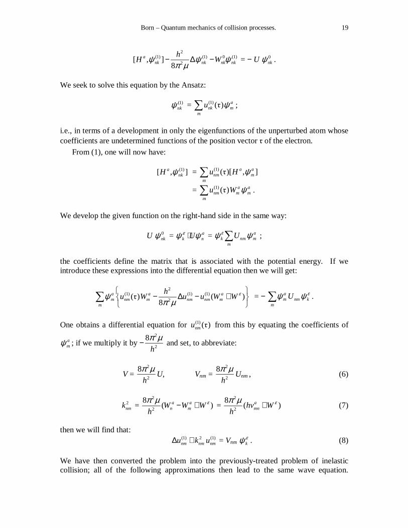
Born – Quantum mechanics of collision processes. 19
2(1) (1) 0 (1)
2[ , ]8
ank nk nk nk
hH Wψ ψ ψ
π µ− ∆ − = − U 0
nkψ .
We seek to solve this equation by the Ansatz:
(1)nkψ = (1)( ) a
nk mm
u ψ∑ r ;
i.e., in terms of a development in only the eigenfunctions of the unperturbed atom whose coefficients are undetermined functions of the position vector r of the electron.
From (1), one will now have: (1)[ , ]a
nkH ψ = (1)( )[ , ]a anm m
m
u H ψ∑ r
= (1)( ) a anm m m
m
u W ψ∑ r .
We develop the given function on the right-hand side in the same way:
U 0nkψ = a
k nUεψ ψ⋅ = ak nm m
m
Uεψ ψ∑ ;
the coefficients define the matrix that is associated with the potential energy. If we introduce these expressions into the differential equation then we will get:
2(1) (1) (1)
2( ) ( )8
a a am nm m nm nm m
m
hu W u u W Wεψ
π µ
− ∆ − +
∑ r = − am nm k
m
U εψ ψ∑ .
One obtains a differential equation for (1)( )nmu r from this by equating the coefficients of
amψ ; if we multiply it by −
2
2
8
h
π µ and set, to abbreviate:
V = 2
2
8
h
π µU, Vnm =
2
2
8
h
π µUnm , (6)
2nmk =
2
2
8( )a a
n mW W Wh
επ µ − + = 2
2
8( )a
mnhv Wh
επ µ + (7)
then we will find that:
(1) 2 (1)nm nm nmu k u∆ + = Vnm k
εψ . (8)
We have then converted the problem into the previously-treated problem of inelastic collision; all of the following approximations then lead to the same wave equation.

Born – Quantum mechanics of collision processes. 20
However, the difference between this problem and the former one is the following: Every transition (n → m) of the atom corresponds to a special differential equation whose right-hand side is determined from the corresponding matrix element of the potential energy. Moreover, another value knm that corresponds to the energy:
nmWε = 2
228 nm
hk
π µ = a
nmhv + Wε (9)
enters in place of the k-value of the incoming wave. The basic qualitative law of electron collisions already follows from that: The energy of the electron after the collision is, in general, not equal to the energy before the collision, but differs from it by an energy jump
anmhv of the atom. A probability function:
Φnm = π2 2 2
0| ( ) |nm nmk f k∞ − s (10)
belongs to any collision process that one can calculate with the help of formula (12) or (13), § 6. § 8. Physical consequences. We next show that our formulas correctly duplicate the qualitative behavior of atoms under collisions, and thus, the fact of “energy jumps,” which has always been regarded as the basic pillar of quantum theory, as well as the most egregious contradiction to classical mechanics. We order the energy levels of the atom by their magnitudes:
0aW < 1
aW < 2aW < …
The index 0 then denotes the normal state, and one has:
anmhv = a a
n mW W− > 0 for n > m.
We next consider the case in which the atom is initially in the normal state. One then has that all a
nmv > 0, and it will follow from (9), § 7 that:
0mWε = Wε − 0amhv .
Now, if Wε < 10
ahv then 0mWε would be negative for m > 0, which is impossible; thus, one
must have m = 0, so:
00Wε = Wε.
One then finds “elastic” reflection with the profit Φ00 . If one lets Wε increase until:

Born – Quantum mechanics of collision processes. 21
10ahv < Wε < 20
ahv
then 0mWε will become only positive for m = 0 and m = 1; one then has either elastic
reflection with the profit Φ00 or stimulated resonance with the profit Φ01 . If Wε increases further until:
20ahv < Wε < 30
ahv
then there will be three cases: Elastic reflection with profit Φ00 , stimulation of the first quantum jump with Φ01, stimulation of the second quantum jump with Φ02 . One proceeds further in the same way. We now fix out attention on the fact that the atom is initially in the second quantum state (n = 1); one will then have 10
av > 0 and 1amv < 0 for m = 2, 3, …
One then has: 10Wε = Wε + h 10
av ,
11Wε = Wε,
1mWε = Wε − h 1amv , m = 2, 3, …
Now, if Wε < h 21
av then 1mWε will be negative for m = 2, 3, …; therefore, there is only
either a collision of the second kind with an energy increase for the electron by h 10av , with
a profit of Φ10 , or elastic reflection with the profit Φ11 . If one has:
21ahv < Wε < 31
ahv
then the stimulation of the state n = 2 with the profit Φ12 will enter into these processes. One proceeds further in the same way. In the general case, if the atom is initially in the state n then there will be only collisions of the second kind for:
Wε < 1,an nhv + ,
for which, the atom will drop into the states 0, 1, …, n – 1 and give up the energy values h 0
anv , h 1
anv , …, h , 1
an nv + , to the electron, with the profits Φn0 , Φn1 , …, Φn, n−1, and the
elastic reflection Φnm . If Wε increases over 1,an nhv + then there will be stimulations with
the profits Φn, n+1, Φn, n+2, …, Φn, m when:
1,an nhv + < Wε < 1,
am nhv + .
The next problem would be to discuss the formula (10), § 7 for the profit; thus, we would like to content ourselves with an entirely tentative, if not truly debatable, consideration.

Born – Quantum mechanics of collision processes. 22
We assume that the potential U can be developed in powers of r−1; for a neutral atom, one will then have the dipole terms:
U(x, y, z) = 3
e
r(Pr) (1)
in the first approximation, where P(q) is the electric moment of the atom. We then
associate it with the matrix Pnm . From (6), § 7, one will then have:
Vnm = 2
2 3
8nm
e
h r
π µ
rP . (2)
Naturally, this Ansatz can only be correct for electrons that pass by the atom at the distance considered. We therefore restrict our consideration to electrons for which r > r0 (1), and thus write, from (13), § 6:
0 ( )nmf k∞ − s = 0
2
1 ( ) ( )
4nm nmi k i k
nm nmrnm
d F e F eik
ρ ρρ ρ ρ ρπ
∞ − − −∫ s s .
We now assume that that the incoming electrons define a parallel bundle, which corresponds to a plane wave; one will then have:
Fnm(r s) = Vnm zike ρs = 2
2 2
8( , )
zik
nm
e e
h
ρπ µρ
s
P s .
Moreover, one will have:
i π knm 0 ( )nmf k∞ − s = 4π 2
e
h
µ(Pnm, s) A, (3)
for which, with sz = cos ϑ, one will have:
A = 0r
dρρ
∞
∫ cos [r (k cos ϑ – knm], (4)
or A = − Ci (r0 [k cos ϑ – knm]), (5)
in which Ci(x) means the integral cosine (2). From (10), § 7, the profit function then becomes:
(1) The exclusion of the central collisions means the temporary sacrifice of being able to interpret an especially interesting group of phenomena, namely, the penetrability of the atom for slow electrons (viz., the Ramsauer effect). (2) S. E. Jahnke and P. Emde, Funktionentafeln, Leipzig, 1909, pp. 19.

Born – Quantum mechanics of collision processes. 23
Φnm = 2 2 2
4
16 e
h
π µ | Pnm , s |2 A2. (6)
If one finally takes the mean over all positions of the atoms then the mean value of the product of two components of Pnm will vanish, and the mean value of the square of the
components will be equal to 12 | Pnm |2, where P means the magnitude of the electric
moment. One thus obtains:
Φnm = 2 2 2
2
16
3
e
h
π µ | Pnm |2 A2. (6)
We would like to discuss this expression for the profit function briefly. One first sees that in our approximation, the profit is proportional to | Pnm |2; i.e., for m ≠ n, to the coefficients of the transition probability bnm of Einstein’s theory of radiation, which corresponds to the processes of absorption and stimulated emission in the radiation
processes (but not with the probabilities of spontaneous radiation anm = 3
3
8 nmhv
c
π bnm) (1).
The profit for elastic reflection is proportional to | Pnm |2, which is a quantity that is not optically effective. The diagonal elements of the matrix Pnm will be zero, in general (2); namely, in addition to the small number of cases in which a linear Stark effect exist (as for the hydrogen atom). Pauli has informed me that he could even derive the vanishing of the diagonal elements of the quadrupole and higher moments for the s-terms of the alkali metals and the normal states of the noble gases and rare earths, which is a result that represents the exact expression for a spherically-symmetric domain of action of the atom. Our approximation thus does not suffice for the calculation of the elastic reflections, for which, one must carry out the approximation to one step further. That should be done next in order to arrive at the possibility of testing our theory for the large body of observations (Lenard and others) of free path lengths of electrons in unexcited gases. Without precise calculation, one can then see that the profit will be determined by terms that are of fourth order in Pnm . Naturally, these terms are much smaller than |Pnm|2. From that, we can understand that the normal cross section of atoms (n = 0) for slow electrons is much smaller (with the order of magnitude of “gas kinetics”) than it is for fast electrons, which can be stimulated (3). The dependency of the profit upon direction will be determined by the function A2 according to (5). It obviously corresponds to a diffraction phenomenon. This consequence of de Broglie’s theory was pointed out about a year ago by W. Elsasser (4). When he seriously considered the wave picture, he concluded that the slow
(1) See J. H. van Vleck, Phys. Rev. 23 (1924), 330; Journ. Opt. Soc. Amer. 9 (1924), 27. M. Born and P. Jordan, Zeit. Phys. 33 (1925), 479. (2) For the harmonic oscillator, e.g., they are zero, but they are present for the anharmonic oscillator. (3) One finds literature on this in the book that appeared just recently by J. Franck and P. Jordan, Anregung von quantensprüngen durch Stöße (Berlin, J. Springer, 1926). (4) W. Elsasser, Die Naturwiss. 13 (1925), 711. The order of magnitude relationship that Elsasser’s argument founded rests upon the de Broglie formula for the wave length:

Born – Quantum mechanics of collision processes. 24
electrons must be deflected by atoms in such a way that their distribution after the collision might correspond to the intensity of the light that is diffracted by a small sphere (1). He coupled it with the observations of Ramsauer on the free path length of electrons (2) and the experiments of Davisson and Kunsman (3) in the angular distribution of electrons that were reflected from a platinum plate. In the meantime, the validity of the argument has been confirmed by experiment by Dymond (4), who observed the appearance of interference maxima for reflected electrons in helium directly. A test of our formula for the general body of observations shall result later. § 9. Concluding remarks. On the basis of the foregoing arguments, I would like to go into the meaning of the statement that quantum mechanics allows one to formulate not only the problem of stationary states, but also that of transition processes. The Schrödinger picture thus seems to be by far the easiest picture to calculate in; moreover, it makes it possible to preserve the usual conceptions of space and time, in which the events play out in a completely normal way. By contrast, the proposed theory does not correspond to the consequences of the causal determinacy of the individual events. In my tentative communication, I have emphasized this indeterminacy in particular, since it seems to me to be in the best agreement with the practice of experimenters. However, it is naturally indefensible (if one would not like to reassure oneself) to assume that it will give further parameters that have still not been introduced into the theory that would determine the individual events. In classical mechanics, they would be the “phases” of the motion – e.g., the coordinates of the particles at a certain moment. It seems at first improbable to me that one could insert quantities into the new theory informally that would correspond to these phases; however, Frenkel has informed me that this can perhaps happen. Be that as it may, this possibility would change nothing in the practical indeterminism of collision processes, since one cannot give the values of the phases; moreover, they must lead to the same formulas as the “phase-less” theory that is proposed here. I would like to believe that the laws of motion of light quanta can be treated in a completely analogous way (5). However, as in the basic problem of the free radiation, one would not have a temporally-periodic process, but a deflection process, and thus, not
λ = 2k
π =
2
h
Wµ.
For 300 volt radiation, one has roughly λ = 7 ⋅⋅⋅⋅ 10−9, and thus waves of atomic dimensions. (1) See K. Schwarzschild, Sitzungsber. d. Kgl. Bayer. Akad. d. Wiss. (1901), 293; G. Mie, Ann. d. Phys. 25 (1908), 377; P. Debye, Ann. d. Phys. 30(1909), 57. (2) C. Ramsauer, Ann. d. Phys. 64 (1921), 513; 72 (1923), 345. For further literature see Ergebnisse der exacten Naturawissenschafter, 3 Bd. (Berlin, J. Springer, 1924), the article of R. Minkowski and H. Sponer, pp. 67. (3) Davisson and Kunsman, Phys. Rev. 22 (1923), 243. (4) Dymond, Nature. (To appear; I am grateful for a glimpse of that work in a letter that Dymond sent to J. Franck.) (5) The complications that have been found up to now regarding the introduction of “ghost fields” into optics seem to me to be based, in part, upon the tacit assumption that the center of the wave and the particle that it determines are at the same place. However, from the Compton effect, this is certainly not the case, and indeed will never be true, in general.

Born – Quantum mechanics of collision processes. 25
a boundary-value problem, but an initial-value problem for the coupled wave equations for the Schrödinger ψ-quantity and the electromagnetic field. Finding the law of this coupling is certainly one of the most pressing problems; as I am aware, it has been addressed in several places (1). Once that law has been formulated, it will perhaps be possible to devise a rational theory of the lifetimes of states, the transition probabilities for radiation processes, and the damping and line widths.
_____________
(1) See, e.g., the soon-to-appear treatise of O. Klein, Zeit. Phys. 37 (1926), 895.