quantum statistics in nonlinear optics
TRANSCRIPT
Chapter 5
QUANTUM STATISTICS IN NONLINEAR OPTICS
J. Mostowski*
Joint Institute for Laboratory Astrophysics University of Colorado
Boulder, Colorado
and
M . G. Raymer
Department of Physics and Chemical Physics Institute University of Oregon
Eugene, Oregon
1. Introduct ion 188
2. Quantized Electromagnetic Field and its Measurement 189
2.1. Field Quant izat ion 189
2.2. Pho ton Flux and Optical Power Spectrum 192
2.3. Flux Power Spectrum 193
3. Q u a n t u m Fluctuat ions in Stimulated Raman Scattering 196
3.1. Raman Medium 196
3.2. Solutions of SRS Equat ions 200
3.3. Average Pho ton Flux of SRS 201
3.4. Power Spectrum of the Stokes Field in the Steady State 204
3.5. Temporal Coherence 206
3.6. Fluctuat ions of the Stokes Field 208
3.7. Temporal Fluctuat ions 211
4. Q u a n t u m Fluctuat ions in Optical Parametr ic Amplification 214
4.1. Optical Parametr ic Amplification 214
4.2. Spectrum and Pho ton Flux of Ο Ρ Α 218
4.3. Ο Ρ Α Intensity Fluctuat ions 220
4.4. Noise Reduction and Squeezing 222
4.5. Homodyne Detection of Fie ld-Quadra ture Noise 225
4.6. Experimental Realization of Pho ton Noise Reduction by Traveling-Wave
Parametr ic Amplification 227
Acknowledgments 232
References 232
* Permanent address: Institute of Physics, Polish Academy of Sciences, Warsaw, Poland
C O N T E M P O R A R Y N O N L I N E A R OPTICS 187 Copyright © 1992 by Academic Press, Inc. All rights of reproduction in any form reserved.
ISBN 0-12-045135-2

188 J. Mostowski and M. G. Raymer
1. I N T R O D U C T I O N
Quantum effects that arise in strong-beam propagation in nonlinear optical media have been recently observed. The study of such effects is a rapidly developing field now, in both experiment and theory.
In treating such problems, it is important to make a connection with semi-classical wave equations used commonly in classical nonlinear optics, and quantum-field operator formalism used in quantum optics. Actually, both methods were applied in the late 1970s to treat superfluorescence from a collection of inverted two-level atoms in the absence of any resonant cavity that would define spatial modes [ 1 - 4 ] . It is well-known that the Heisenberg equations for quantum fields are identical to Maxwell's equations coupled with material equations [ 5 - 7 ] . An advantage of making this connection is that one can exploit intuition about classical wave propagation in the study of quantum propagation. This includes group-velocity dispersion, phase match-ing, transient effects, temporal and spatial coherence properties, etc.
This chapter will discuss two important examples of propagation pheno-mena: stimulated Raman scattering (SRS), and squeezed light generation by traveling-wave, optical parametric amplification (OPA). In both cases, a pump laser pulse enters a nonlinear medium, and spontaneous generation and amplification lead to a macroscopic pulse at a frequency different from the pump. At low temperature, purely classical electromagnetic theory cannot account for the initiation of the scattering due to the lack of a medium polari-zation oscillating at frequencies other than that of the pump. The generated pulse, which has large intensity, is amplified zero-point noise (associated with the field and /or medium). SRS is an example of a gain process, i.e., phase-insensitive process, while ΟΡΑ is a parametric, i.e., phase-sensitive, amplifi-cation process. The importance of this distinction has been emphasized recently [8] .
The main implication is that SRS can be described by an effective classi-cal, stochastic process for the purpose of understanding its photodetection, whereas Ο Ρ Α leads to intrinsically quantum effects, including sub-shot noise [9], squeezing [10,11], etc. Nevertheless, even the SRS effect is a quantum one; the energy shows macroscopic fluctuations [12] and the noise strength in the equivalent classical theory is proportional to h [13].
These two cases were chosen in order to illustrate the difference in physical phenomena occuring in two classes of traveling-wave light amplifiers. Many nonlinear quantum effects are also known to occur in resonant optical cavities; these will not be explicitly discussed here since they have been reviewed several times previously [ 1 4 - 1 7 ] .
Section 2 presents a discussion of fluctuations of the quantized electro-magnetic field. This basic formalism is applied to SRS and OPA in Sections 3 and 4, respectively. These two sections can be read independently.

5. Quantum Statistics in Nonlinear Optics 189
2. Q U A N T I Z E D E L E C T R O M A G N E T I C F I E L D A N D ITS M E A S U R E M E N T
2.1 . Field Quantization [ 5 - 7 ]
This section deals with fundamental concepts of the electromagnetic field, and its measurement by means of photoelectron counting. Fundamental concepts relating to the quantized electromagnetic field will be introduced, and they will be used later in the study of electromagnetic fields interacting with matter. Further, the photon flux, optical spectrum, and photon flux spectrum will be defined. These quantities are measurable by means of photo-electron counting, and provide a method of determining the statistical prop-erties of the electromagnetic field.
The electromagnetic field is described by two vector fields, the electric field E(i,r) and the magnetic induction B(f,r). At each space point r, the quantities E(r, r) and B(r, r) are operator variables. It is convenient to use creation and annihilation operators a(k, λ) and a
f(k ,A) to describe the field. The transfor-
mation from E(i,r) and B(i,r) to a(k,A) and af(k,À) involves Fourier trans-
forms. Since the Fourier transform will be used extensively in this chapter, we will give the basic definitions here.
The temporal Fourier transform of a function or operator/(f) is defined as
/ ( ω ) = J dtexp(iœt)f(t), (1) - o o
and will be consistently denoted by the tilde symbol. The inverse transform is
00
1 dœexp( — iœt)f(œ). (2)
Of interest will be also the analytic signals: The positive-frequency part
OO
1 /<*<·->= 2„
and the negative-frequency part
άω exp( — iœt) / (ω), (3)
f(-\t) = i - j dœexp( + iœt)p(œ). (4)
The transformations between the fields E(i, r) and B(r, r) and the operators
190 J. Mostowski and M. G. Raymer
a(k, λ) and aT(k , / ) are given by spatial Fourier transforms:
λ E(f,r) =
B(i,r) =
(2π)3
1
( 2 ^
d3kΣ ^(k)e(k, λ) e x p ( - icot + /k · r) a(k, / ) + h.c , (5)
d3/ c£#(k ) —- χ e(k , / l)exp(-/coi + ik · r )a (k , / ) + h.c , (6)
where e(k, / ) denotes the polarization vector labeled by polarization index A, and the frequency ω is connected with wavevector k by ω = c\k\. The function g(k) is given by g(k) = — i(hc\k\)
1/2. The part of the field proportional to the
annihilation operator involves positive frequencies only. It is thus an analogue of the positive-frequency analytic signal, Eq. (3). The commutator between a(k, λ) and a
f(k, λ) is
[ a ( k , λ \ a\k\ / ' ) ] = ΐ(2π)3 δ
3(k - k ' ) . (7)
In many optical applications, only a narrow band of frequencies and wavevectors is of interest. The paraxial approximation to the wave equation is a formalization of these ideas. Suppose that we are interested in a laser beam of frequency ω propagating in the direction parallel to a vector K. Often, it will be assumed that the direction of propagation coincides with the ζ axis. Of course, a laser beam cannot be purely monochromatic; the frequency ω should be considered as a central frequency allowing for some frequency spread. Also, because of diffraction, the direction of propagation is not perfectly defined; the light beam spreads around the central direction of propagation. In order to describe a beam, we will write the vector k as
k = Κ + q, (8)
where ω = c\K\ and the vector q, which describes the spread in wavevectors, has length much smaller than the vector K. The expansion Eq. (5) takes the form
(2π) d3g£#(K)€(q ,A)exp[ - /<^ i + + Q) · r M q > ^ ) + h.c , (9)
where c(q, λ) = a(K + q, λ) and e(q, λ) = e(K + q, λ). Since |K + q |
1 /2 varies slowly for |q| « |K|, we have approximated the
function g(k) by its value at the central vector K: g(k) = g(K). Two quantities that will be of interest to us are the positive- and negative-
frequency parts of the electric field. By definition, the positive-frequency part, denoted by E
( + )(r,r), is the part that is proportional to the annihilation
operators. The remaining part, denoted by E( _ )
( i , r ) , is called the negative-frequency part of the field.
We will expand the frequency |Κ + q | in q up to the second order. Denote by q L and q T the parallel and perpendicular components, respectively, of q
5. Quantum Statistics in Nonlinear Optics 191
relative to K. Then, IΚ + q| ^ |K| + |q L| + q | / (2 |K|) + q£/(2|K|). We now will neglect the term |q L|
2/ (2 |K|) as compared to |qL| , but retain the term q | /(2 |K|).
This is the quantum version of the slowly-varying-envelope approximation (SVEA). In this approximation, the field operators are related to creation and annihilation operators by Eq. (9) rather than Eq. (5), but otherwise the struc-ture of the theory remains unchanged.
It is important to know the commutation relations for the vector com-ponents of the electric field in the SVEA at different space points at the same time. Straightforward calculation gives
[E;.+»(i,n), r2 ) ] = l 0 ( K ) |
2( \ j - ^ ) e x p [ / K · ( r , - r 2 ) ] S
3{TL - r 2 ) .
V K J (10)
In order to get this result, we have extended the range of integration to all values of q. This can be done provided the distance between the points rl and r 2 is much larger than the inverse of the maximal value of |q|. Thus, the approximation introduced does not allow one to study the behavior of the fields at short distances.
In the slowly-varying-envelope approximation, the electric field satisfies the approximate version of the wave equation:
2i^i - ϋκξ- + V*)v + )
(t,z) = 0, (11) dt dz
where ζ is the direction of Κ and Vj is the transverse part of the Laplacian. In this chapter, we will discuss effects in which the diffraction plays a
marginal role only. We will therefore neglect the transverse part of the Laplacian. The remaining part of the wave equation contains the ζ derivative only. In other words, such an approximation reduces the problem of wave propagation to a purely one-dimensional problem. This is an important case, and will be discussed more carefully.
Suppose the electromagnetic field is restricted to a pencil-shaped volume with the transverse cross sectional area equal to A. Suppose, moreover, that the field does not change much across the transverse cross section. In such a case, one may introduce the average field, which depends on the longitudinal coordinate only:
1 d
2pE(t,z,p). (12)
The decomposition of the average field into plane waves takes now the form
E(i,z) = i — Yg(K)€(K,À)expl-iœt + i(K + q)z]c(q,k) + h.c , (13) 2π A
where q now denotes the one-dimensional wavevector, c(q, X) = c(q, q T ~ 0 , λ).

192 J. Mostowski and M. G. Raymer
The Hamiltonian for the electromagnetic field can be expressed in terms of the one-dimensional creation and annihilation operators as
A ^ Σ ^ ( * , λ ) φ , 4 (14) 2π Λ
This one-dimensional Hamiltonian generates one-dimensional equations of motion. In all cases discussed, we will not consider polarization changes; electric fields will have one polarization component only. We will therefore skip the polarization index λ. The procedure of neglecting electric-field po-larization and restricting the propagation to one dimension only leads to a simplified, scalar version of electrodynamics. In this case, the commutation relation for the field operators is
[£< + >( t,z),£<->(f',z')]
2 n hw Ζ
-1 ί' — c
(15a) cA
where ω denotes the central frequency. In the frequency domain, this becomes
[£(v,z), £f(v ' , z ' ) ] - 2n^^jô(v - v ')exppv(z - z')/c]. (15b)
The electromagnetic fields discussed in this chapter are not free fields, but are generated by sources. It is the polarization of the medium that usually provides such a source. In this case, the slowly-varying-envelope field satisfies an equation that is a direct consequence of the wave equation with a source for the electric field:
2i™l + 2iKplE< +
%z)= -%ω2Ρ^%ζ). (16)
"z dt dz J c
z
Here P( + )
(r,z) = Nex{ + )
denotes the slowly varying envelope of the positive-frequency part of the medium polarization oscillating with central frequency ω, where N, e, and
+ ) are respectively the density, charge, and coordinate of
electrons. It should be pointed out that there are some subtle questions that arise when a nonlinear, dispersive dielectric is quantized, having to do with the proper choice of conjugate canonical variables. Reference 18 should be consulted for a discussion of using the macroscopic fields, rather than the microscopic fields as was done here.
2.2. Photon Flux and Optical Power Spectrum
The electric field at optical frequency varies too fast in time to be measured by any macroscopic device. Instead, slowly varying quantities such as photon flux, optical power spectrum, and flux power spectrum are measured in typical optical experiments.

5. Quantum Statistics in Nonlinear Optics 193
The operator corresponding to total flux (photons per second) in a quasi-monochromatic, quasi-collimated beam with cross-sectional area A and center frequency ω, is
cA / ( 0 = 2 ^ — ζ ) £
< + )( ί , 4 (17)
The expectation value of the photon flux as just defined is measured by photocounters by counting the average number of photoelectrons due to impinging photons.
The spectrum of light provides information about the frequency com-position of the light beam. The optical spectrum is the power spectrum of the field fluctuations. It is denoted by S(v), where ν is an angular frequency, and is defined by
CE(T)e^dz, (18)
where the two-time field autocorrelation function is
C £( T ) = < £(- > ( Î , Z ) £
( + )( Î + T , Z ) > , (19)
and is assumed not to depend on t in the case of stationary fields. The integral of the spectrum over frequency equals the total average flux:
</> = S(v)dv. (20)
It is often convenient to express the spectrum in terms of the two-frequency field correlation function, defined in terms of the Fourier transform of the field operator. It is easy to show for a stationary process that
2(2nhœ^
~c~Ä <£t(v,z)£(v',z)> = 4 π
2( )S(v)ô(v - ν'), (21)
where the transforms are defined as in Eq. (1). This formula gives an alternative way of calculating the power spectrum.
2.3. Flux Power Spectrum
Additional characterization of the light beam can be found by measuring the flux power spectrum. As will be shown in Section 4, squeezing of light can be observed by measuring this spectrum. For a steady-state light source, the intensity typically fluctuates on a time scale of the order of the inverse optical bandwidth. This leads to fluctuations of the photocurrent from an optical

194 J. Mostowski and M. G. Raymer
detector. A common way to observe such fluctuations is with a radio-frequency (rf) spectrum analyzer, which measures the Fourier transform of the photo-current during some long time period. If the photodetector has unit quantum efficiency, then every incident photon produces one electron. In this case, the statistical properties of the photoelectrons are identical to those of the photons. We will treat this case for simplicity. Strictly speaking, a rigorous treatment is based on the probabilities of producing various numbers of photoelectrons; it reduces to our simple version for unit detector efficiency [ 1 9 - 2 1 ] .
Theoretically, the power spectrum P(v) of the photon noise is evaluated as the Fourier transform of the two-time autocorrelation function of the photon flux noise:
P(v) C,{x)e"zdT, (22)
where the flux autocorrelation function is
Q ( T ) = < Γ Δ / ( ί ) Δ / ( ί + τ)>
[<T£<->(t,z)£< + >(t,z)
_ ( cA ^2
\2nhcol
χ E{-\t + τ , ζ )£
( + )(ί + τ,ζ)> - <£
(->(ί, ζ ) £
( + )(ί, z )>
2] . (23)
The brackets indicate a quantum expectation value and the quantity AI(t) = I(t) — </(i)> is the deviation of the photon flux from the mean value. The electric field operator is to be evaluated at the detector. This formula ap-plies to fields with bandwidth narrow compared to the optical frequency. The symbol Τ indicates time ordering [19], which is defined by
TE^(t29z)E{-\tuz) = E<-\tl9z)E<->(t2,z) (t, < t2)9
(24)
T& +
\tl9z)E< +
\t29z) = E^(t29z)E^(tl9z) (t, < t2).
Before applying the time ordering in Eq. (23), the field commutator equa-tion (15) is used to put the fields in the normal order:
+ + It is
important to note that the ordering refers to the field at the detector, not, for example, at the input to the nonlinear medium. The correlation function becomes
Q W = {TE'-\t9z)E^\t + τ,ζ)£< + >(ί + τ,ζ)Ε<
+ >(ί,ζ)>
+ < / > < 5 ( τ ) - < / >2. (25)
5. Quantum Statistics in Nonlinear Optics 195
The effect of the time-ordering operator in this equation is to leave the operators as written for τ > 0 and to move the τ variable to the outside positions of the expectation value for τ < 0. This equation can be written compactly for arbitrary τ as
CJ(T) = </>(5(τ) + <Τ :Δ / ( ί )Δ / ( ί + τ):>, (26)
where the double dots indicate normal ordering at the detector. This means that all annihilation operators are placed to the right of all creation operators in the expectation value. The first term in Eq. (26) is the shot noise associated with the random generation of discrete photoelectrons in the detector. The second term is the noise in excess of the standard shot noise, and is called wave noise. It is associated with the classical-like fluctuations of the electric field amplitude. The shot-noise level was believed until recently to be the lower bound for noise in photodetection. In many applications, it imposes a limit to the sensitivity of optical measurements.
For the case of an ideal, monochromatic, coherent light beam, i.e., a single mode in a coherent state, the wave-noise term is zero, and only the shot noise is present. The flux power spectrum is then simply
PcoM = </>, (27)
that is, white noise with spectral density (per radian/second) equal to the average photon flux. The detector has been assumed to have infinite bandwidth. Actually the power spectrum should be multiplied by the detector frequency-response function, which rolls off at high frequency [19].
For thermal light, it is well-known that the higher-order correlation func-tions can be expressed in terms of the two-point correlation function [22]. This is the quantum analog of the Gaussian moment theorem in classical random processes [23]. Thus, the flux correlation can be expressed in terms of the field correlation as
C, (T ) = < / > δ(τ) + ^-J\CE{x)\2. ( 2 8 )
This implies that, for thermal light, the rf flux spectrum is given in terms of the optical spectrum as
^Th(v) = </> + 2π J d v ' S i v W - v). (29)
This illustrates that the fluctuations at frequency ν arise from temporal beating between spectral components at v' and v' — v. Note that the flux noise density is greater than the shot-noise level at all frequencies. This is characteristic of so-called classical light. Later, we will see a case of nonclassical light where the noise density is less than the shot-noise level.
196 J. Mostowski and M. G. Raymer
3. Q U A N T U M F L U C T U A T I O N S IN S T I M U L A T E D R A M A N S C A T T E R I N G
In this section, stimulated Raman scattering will be discussed as an example of phase-insensitive amplification. The Raman effect is one of the first discov-ered and best-known nonlinear optical processes. It is used as a tool in spec-troscopic studies, and also in tunable laser development, high-energy pulse compression, etc. Several review articles exist that summarize the earlier work on the Raman effect [24,25] . Here, we will concentrate on the quantum nature of the process (reviewed in detail in [25]), and discuss its implications.
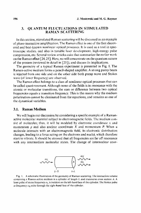
The geometry of a typical Raman experiment is presented in Fig. 1. The Raman-active medium forms a pencil-shaped amplifier. A strong pump beam is injected from one side and on the other side both pump wave and Stokes wave (of lower frequency) are observed.
The Raman effect belongs to a class of nonlinear optical processes that can be called quasi-resonant. Although none of the fields is in resonance with the atomic or molecular transitions, the sum or difference between two optical frequencies equals a transition frequency. This is the reason why the medium polarization cannot be eliminated from the equations, and remains as one of the dynamical variables.
3.1 . Raman Medium
We will begin our discussion by considering a specific example of a Raman-active molecular material subject to electromagnetic fields. The medium con-sist of molecules; thus, it will be modeled by electronic coordinate χ and momentum ρ and also nuclear coordinate X and momentum P. When a molecule interacts with an electromagnetic field, its electronic distribution changes, leading to a force acting on the electrons and nuclei, which therefore start to vibrate. It should be stressed that all frequencies are far off resonance with any intermediate molecular states. The change of internuclear coor-
I ι z=0 z=L
Fig. 1. A schematic illustration of the geometry of Raman scattering. The interaction volume containing a Raman-active medium is a cylinder of length L and transverse cross section A. A laser pulse of mean frequency coL is incident on the left-hand face of the cylinder. The Stokes pulse at frequency cos exits through the right-hand face of the cylinder.
5. Quantum Statistics in Nonlinear Optics 197
dinates leads to a change of the electronic polarizability. The whole process is described by the following Hamiltonian:
H = He + HF + HN + Hint. (30)
The field part HF describes the energy of the free electromagnetic field, as discussed in Section 2. The nuclear part HN describes the vibrations of the nuclei in the molecule, and for low vibrational levels is given by a harmonic oscillator Hamiltonian:
ffN = P2/2M + (KN/2)X\ (31)
and the resonance frequency is ωκ = ( K N / M )1 / 2
. In the dipole approxi-mation, the interaction part is the energy of the electronic polarization in the presence of the electric field E:
Hint=-exE, (32)
where e is the charge of the electron and χ is the displacement of the electron from the equilibrium position. The electronic Hamiltonian is taken to be that of a harmonic oscillator. This is the Lorentz model for electronic motion, and is valid for weak excitation. The molecules are Raman active if the restoring force acting on the electron depends on the internuclear separation X, thus providing a coupling between the nuclear and the electronic motion. Hence, the electronic energy is
He = p2/2m + k(X)x
2/2 = p
2/ 2 m + m | > e ( X ) ]
2x
2/ 2 , (33)
where m is the electron mass and œe(X) is the resonant frequency. In the Raman problem, the electric field consists of two parts, well separated
in frequency. The first component, which is called the pump (or laser) field, has a frequency coL not very close to any electronic resonance frequencies. The pump field is assumed to be strong, and we will not take into account its changes. In other words, we will treat it as an external classical field, not being affected by the interaction. The second component of the electromagnetic field is called the Stokes field. Its frequency œs is such that
ajs = œ h - œ R . (34)
Thus, the field is written as a sum of two components:
Ε = E(
L
+)e-
icou + E
{
s
+)e-
ic)st + h.c. (35)
It is the Stokes wave we will be mostly interested in. A wave at the Stokes frequency may be injected into the Raman-active medium; in this case, it will be amplified, or, what is more interesting to us, the Stokes wave may be spontaneously generated by the medium without any injected signal. In order to describe the spontaneous generation of the Stokes field, we must use the
198 J. Mostowski and M. G. Raymer
quantum theory of the electromagnetic field as well as the quantum theory of matter.
We will proceed with a discussion of the equations of motion derived from the Hamiltonian, Eq. (30). We start with the equation of motion for the electronic coordinate, in the Heisenberg picture:
x = -œl{X)x + (e/m)E, (36)
where coe(X) = >Jke(X)/m is the electronic resonance frequency. Since the field does not contain frequency components in resonance with the electronic frequencies, the molecular coordinate oscillates with the frequency of the driving fields. Thus, after introducing the positive- and negative-frequency components of x:
x = x ^ e -i < au
+ x{
s
+)e-
i(0st + h .c , (37)
Eq. (36) is solved adiabatically to give
ex(
L
+) = oc(X)E
(
L
+\ (38)
where the electronic polarizability α depends on internuclear coordinate:
a(X) e
2
2m<we(X)
1 1
+ _o>e(X) - fflL coe(X) + cuL
(39)
The internuclear coordinate and momentum obey the Hamiltonian equa-tions of motion in the Heisenberg picture. The interaction energy appearing in these equations now depends on x. The internuclear coordinate thus obeys
χ = _ ω 2 χ + _L J _ ίβχ(Χ)ΕΙ (40)
Following the standard adiabatic procedure, we now insert the expression for χ (Eq. (38)), neglect all off-resonance terms, and neglect terms corresponding to frequency shifts (ke(X)x
2) [27] . Representing the nuclear motion in terms of
slowly varying variables:
χ = Qîe-i(ORt
+ h .c , (41)
we find the central equation of motion for the Raman problem:
o'-sbs^)^"' , 4 2 )
Alternative derivations of this equation are given in [26] and [28]. Homogeneous broadening of the Raman transition, due to molecular col-
lisions, is modeled by adding both a term that leads to damping of Q(t) at a
5. Quantum Statistics in Nonlinear Optics 199
rate Γ, and a term representing the random fluctuations due to the collisions:
v-i^iS)*'*-'-™'*™ ,43)
F(t) and its adjoint are quantum-statistical Langevin operators describ-ing the collision-induced fluctuations. They are taken to be delta correlated:
(F\t)F(t')) = 2F(h/2mœRp)ô(t - ί'),
<F(t')F\t)} = 0, (44)
<F(i)F(t')> = 0.
Higher correlation functions are assumed to be derived from Eq. (44) with the help of the Gaussian property. This guarantees that the equal-time commuta-tion relations between the operators Q(t) and Q\t) are preserved [22,26] .
Equation (43) describes the response of a single molecule to the electric field and to collisions. To treat the spatial propagation of the electromagnetic field, it is convenient to formulate the atomic response in terms of collective molecular operators defined as
ß(t,z)=-Zß-(t). (45) The sum is over all molecules lying within a thin transverse slice of the pencil-shaped medium, with thickness Δζ, centered at the longitudinal position z. The average number of molecules η in such a slice is Ν Α Δζ, where Ν is the number density of molecules, and A is the transverse cross-sectional area of the medium. The thickness of a slice is assumed to be much smaller than a Stokes wavelength (Δζ « A s), while the volume of a slice is much greater than a cubic wavelength of the Stokes radiation (A Az » λ$). This justifies the neglect of the near-field dipole-dipole interactions (Νλ$ « 1), while allowing for a continuum description of the medium (NAAz » 1). In the continuum limit, the collective operator has the property
<ßt(0,z')6(0,z")> = (h/2mœRp)ô(z' - ζ"), (46)
where ρ = ΝΑ is the linear density of molecules along the pencil-shaped region. Similarly, the collective Langevin operators F(i,z), F^(t\z'\ defined analogously to Eq. (45), obey
<Ft( i ' , z ')F(i", z")> = 2Y{h/2mœRp) ô(t' - t") δ(ζ' - ζ"), (47)
and the remaining bilinear products have a zero expectation value. The equation describing the evolution of the Stokes field is that for
propagation, as given in Eq. (16). The source of the Stokes field is given by the electronic polarization of the medium at the frequency ω 8 . The polarization,
2 0 0 J. Mostowski and M. G. Raymer
however, can be expressed by the nuclear coordinate Q{t) with the help of Eqs. (38) and (39). Then, writing EL for E
(
L~\
iK2Qi(t,z)EL(t,z),
(48)
Γβϊ ( ί , ζ ) - ÎKlE{
s-\t,z)Et(t,z) + F%z)9
where κχ = (da/dX)/(2œRM) and κ2 = 2n(œs/c)N(da/dX). This set of equations constitutes the formal description of stimulated
Raman scattering (SRS). It should be noted that several effects have been neglected. We treat the pump field as a given external agent and therefore we neglect possible saturation effects. Also, the harmonic-oscillator description of the molecular vibrations does not allow for description of a possible signifi-cant population of the vibrationally excited state. Therefore, the preceding description is applicable to the case when the Stokes field is relatively weak.
The form of Eq. (48) is the same as in semiclassical theories of the stimulated Raman effect [25] . The only difference is the operator nature of both the Stokes field Es and Raman variables Q. We will see that this fully quantum description leads to results not described by semiclassical treatments. Further discussion of these equations can be found in Ref. 26.
3.2. Solutions of S R S Equations
The set of equations (48) for the polarization field and for the electric field can be solved exactly in analytic form for arbitrary time dependence of the laser field EL(t,z) in the case of forward Stokes emission in a dispersionless medium. The initial conditions for the case we are interested in are obtained by noting that, in a dispersionless medium, the laser field £ L( i , z) depends only on the local time variable τ = t — z/c9 and thus a laser pulse whose leading edge is at t = z/c leaves the atomic operator β(τ,ζ) unperturbed for τ < 0. Thus, the initial condition for the operators β(τ ,ζ) (see Eq. (46)) becomes
<ef(t = 0 ,ζ)β(τ = 0,z')> = (h/2mœRp)ô(z - z'\ (49)
where ρ is the linear density of molecules. Also, that the Langevin force is stationary implies that
<Ft( t , Z ) F ( T ' , Z ' ) > = 2T(h/2mœRp) δ (ζ - ζ') δ(τ - τ'). (50)
The initial value for the Stokes field £ S( T , 0) is specified at the input face of the medium, ζ = 0, for all times τ. This means that backward Stokes emission is explicitly ignored. Depending on the initial state of the radiation field, this condition describes either an externally incident Stokes wave, which can
d 1 d
dz c dt
5. Quantum Statistics in Nonlinear Optics 201
experience Raman amplification, or the vacuum field from which Stokes emission can build up.
With these initial conditions, the set of equations has the following solution [28] :
Ε Π τ , ζ ) = - /K2£L(T)exp(
ζ
- Γ τ ) j*dz' Ôf(0 ,z ' )
χ / 0 { [ 4 Κ ικ 2 ( ζ - z ' )p (T) ] 1' 2}
+ (KlK2z)l'2EL(x) ίίτ'εχρ[ —Γ(τ — τ')]
χ £*(T')4~V ,0)
- I K 2 £ L ( T )
, ^ { [ ^ ^ ( p M - p d ' ) ) ]1
'
ζ τ
dz
ο ο
[ Ρ ( τ ) - Ρ ( τ ' ) ] 1 /2
ί ί τ ' β χ ρ [ - Γ ( τ - τ ' ) ] ί ν . ζ ' )
χ / 0 { [ 4 κ ι Κ 2( ζ - ζ ' ) ( ρ ( τ ) - ρ ( τ ' ) ) ]1 / 2
} ·
Here, 4(χ) are modified Bessel functions and
Ρ(τ)
τ
jdT'|£L(t')l3
(51)
(52)
is the power of the laser field integrated up to time τ. This solution was presented in the quantum case first by von Foerster and Glauber [29].
The part of the field that is due to the source, namely, Q!(0, ζ) and F*(τ, ζ),
is proportional to Planck's constant ft, as seen from Eqs. (49) and (50). This shows that the Stokes emission is a quantum process—without the quantum initiation there would be no spontaneous emission of the Stokes field.
3.3 . Average Photon Flux of S R S
Various properties of the Stokes field will be discussed now. The basis of the discussion is the solution (51) to the operator equations describing the field. The results presented in this section follow Ref. 26.
One of the most important characterizations of the Stokes field is the average intensity of the Stokes beam in the forward direction, which may be
2 0 2 J. Mostowski and M. G. Raymer
obtained from Eq. (51) by calculating the normally ordered expectation value of the intensity at the output face of the Raman medium (see Eq. (17)). The units of the intensity are such that Ι8(τ, ζ) gives the average number of Stokes photons emitted per second through the end face of the pencil-shaped excited region into the solid angle A/L
2 defined by the geometry of the region. We will
consider only the case where no Stokes wave is externally incident on the medium, and so we have, for the initial field,
< Ε ^ > ( τ ' , 0 ) 4 + )( τ " , 0 ) > = 0 , (53)
which means that vacuum fluctuations are not detected with a photodetector. Using Eqs. (49) and (50) and the fact that Es, Q\ and F are statistically independent, we find
Ac ft h(
T>
z) 2nhoosp 2mœR
K2^
L^
- ιΐ^κ,κ,ζρ^γΐ2)}
exp( - 2Γτ) { / g( [4/q κ2 ζρ(τ)] 1/2
+ 2Γ dT ' exp [ -2r ( i - τ ' ) ] [ / ^ { 4 κ ^ 2 ζ [ ρ ( τ ) - ρ (τ ' ) ]}1 / 2
)
/ Ϊ ( { 4 Χ ικ 2 ζ [ · ρ ( τ ) - ρ ( τ ' ) ] }1 / 2
) ] (54)
This is a general expression for the Stokes intensity for arbitrary time, Raman gain, and laser pulse shape £ L(T ) . It is applicable when there is no significant depletion of the pump or population of the vibrational excited state of the molecules forming the Raman medium. The consequences of the formula (54) will be studied in some detail in the following, under various limiting conditions.
An important limit of Eq. (54) occurs when the laser intensity is sufficiently low for Raman gain to be negligible, and the atoms scatter light independently and spontaneously. In this limit, the intensity is
hi^z) = - ^ - \ K 2 E L ( T ) \2
Z . (55) 2nnœsp 2mœR
This result shows that the intensity of spontaneous Raman scattering grows linearly with the amplifier length and follows the laser intensity adiabatically. It can be shown that the present treatment exactly reproduces the result for spontaneous scattering based on the conventional Kramers-Heisenberg treatment [26,28]. The energy flux, hcosIs, is proportional to h.
The quantum theory presented here allows us to discuss stimulated Raman scattering with the help of the same basic formula given in Eq. (54). It should be stressed once more that the transition from the spontaneous to
5. Quantum Statistics in Nonlinear Optics 203
the stimulated case is automatically taken into account in this treatment. Two regimes of the stimulated Raman scattering will be distinguished: transient, and steady-state. In the transient regime, the pump pulse is much shorter than the molecular collisional relaxation time whereas, in the steady-state regime, the pump pulse is much longer than the relaxation time.
For times short compared with the molecular collisional relaxation time (Γτ -> 0), only the first term in Eq. (54) contributes, giving, for the transient Stokes scattering at arbitrary laser intensity,
Is(x,z) = \gTz{Il\_{2gzx)1^ - l\ί(29ζτ)^}, (56)
where g = 2K1K2\EL\2/V. We have assumed here that the pump laser pulse
has a square shape. This result can be approximated in the high-gain limit (gz/Γτ » 1 ) :
e x p [ 2 ( 2 ^ z r i ) ^ / s ( T
'z )
= 8 ^ ' ( 5 7)
The dependence of the intensity on the factor 6 χ ρ [ 2 ( 2 # ζ Γ τ )1 / 2
] is reminiscent of the semiclassical result for the transient Raman amplifier [25] . Note that the intensities given by Eqs. (56) and (57) do not depend on the molecular collisional relaxation rate Γ, since Γ appears only in the product gF, and the gain coefficient g is inversely proportional to Γ.
If the pump pulse is much longer than the collisional relaxation time, one is interested in Stokes intensities for times τ much longer than Γ "
1. In this case,
the system has reached the steady state. For times long compared to the molecular relaxation time (Γτ oo), only the second term in Eq. (54) contri-butes, with the upper integration limit taken to infinity. It may be shown that, for square laser pulses,
/ s (oo ,z ) = \gYzll0{gzll) - / ^ z / 2 ) ] exp(^z/2). (58)
In the low-gain limit (gz « 1), this result reduces to the spontaneous scattering intensity, \gYz, while in the high-gain limit (gz » 1), it becomes
Γ / s(oo , z ) ^ — -ïjjexpigz). (59)
2(ngz)llz
This result verifies that g is identified as the steady-state gain coefficient. The dependence on the factor (ngz)~
1/2 is reminiscent of the semiclassical result for
the steady-state Raman amplifier, in the case of a broad-band pump [30]. In Fig. 2, the steady-state Stokes intensity / s( °°>
z) given by Eq. (58), is
plotted as a function of gz, the number of gain lengths in the medium. The transition from spontaneous (linear) growth to stimulated (exponential-like) growth is clearly demonstrated. This result is compared with the standard

204 J. Mostowski and M. G. Raymer
- 2 0 2
log ( gz )
Fig. 2. Steady-state Stokes intensity as a function of gain gz. Curve (a) is the quantum-field
result given by Eq. (58), while curve (b) is the pho ton rate-equation result, | [ exp(#z ) — 1]. The
curves show the transition from linear, spontaneous growth to exponential, stimulated growth.
(From [28]).
predictions of phenomenological photon-rate equations, in which Stokes photons, produced by spontaneous Raman scattering, act as a source for exponential-type stimulated buildup, cf. [6 ,26] .
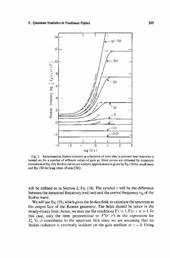
In Fig. 3, we have plotted the time-dependent Stokes intensity IS(T,Z),
evaluated by numerical integration of Eq. (54), for a number of different values of gz. It is seen that for small gain (gz = 0.1, 0.01) the Stokes intensity is a constant, given by the spontaneous scattering result Eq. (55). For larger values of gz, a rapid growth of the intensity is seen at times of the order of Γ
1, the
molecular collisional relaxation time. At longer times (Γτ > gz), a steady-state value is eventually attained, given by Eq. (58).
3.4. Power Spectrum of the Stokes Field in the Steady State
The power spectrum of Raman scattering is an important physical quantity, which depends strongly on the quantum-statistical nature of the generated radiation. It has a meaning in the steady state only. The power spectrum S(v)
5. Quantum Statistics in Nonlinear Optics 205
l og (Γτ)
Fig. 3. Ins tantaneous Stokes intensity as a function of time after a constant laser intensity is
turned on, for a number of different values of gain gz. Solid curves are obtained by numerical
evaluation of Eq. (54). Broken curves are analytic approximat ions given by Eq. (56) for small times
and Eq. (58) for long times. (From [28]).
will be defined as in Section 2, Eq. (18). The symbol ν will be the difference between the measured frequency (rad/sec) and the central frequency œs of the Stokes wave.
We will use Eq. (51), which gives the Stokes field, to calculate the spectrum at the output face of the Raman generator. The fields should be taken in the steady-steady limit; hence, we may use the conditions Γτ » 1, Γ(τ + s) » 1. In this case, only the term proportional to F\x\z') in the expression for £ S
_ )( T , Z ) contributes to the spectrum 5(v), since we are assuming that no
Stokes radiation is externally incident on the gain medium at ζ = 0. Using
206 J. Mostowski and M. G. Raymer
Eq. (51), the Stokes spectrum is found to be
- 1 (60)
This expression will be used to evaluate the Stokes spectrum in several limiting cases. The spontaneous, or low-gain, limit occurs when gz « 1. In this case,
which shows that spontaneous Raman scattering has a spectral width given by the Raman line width Γ.
When the gain becomes high (gz » 1), gain narrowing distorts the Lorentzian line shape by amplifying the center part of the Stokes line more strongly than the line wings. Then, the spectrum becomes spproximately
This formula gives a gaussian shape of the power spectrum with width proportional to T/(gz)
l/2. This is a manifestation of the effect known in non-
linear optics as gain narrowing—the larger the gain, the narrower the spec-trum becomes. The result (62) is similar to that found in the semiclassical treatment of a Raman amplifier with a broad-band input Stokes wave [30].
The flux power spectrum of the Stokes radiation can also be evaluated. The calculation is straightforward, and leads to the result that the flux power spectrum for the Stokes radiation is connected with the optical spectrum as in Eq. (29), the same equation that gives the relation between the two spectra in the case of thermal light.
3.5. Temporal Coherence
Another quantity that characterizes the stimulated Raman process is the temporal coherence of the Stokes field. This can be understood by a procedure that is formally analogous to the one used in classical coherence theory, cf.
A field is said to be coherent in the second order if the two-point correlation function can be factored: < £ ( _ )( τ + S , Z ) £
( + )( T , Z ) > = f(x + s)f*(x), for some
function f(t). The Stokes field is usually not coherent in this sense. Nevertheless, the preceding factorization suggests the use of an eigenfunction representation of the two-point correlation function.
The two-point correlation function (Ei
s~)(z + s , Z ) E
{
S
+ )( T ,Z ) > can be
treated as an integral kernel, and its eigenvalues ÀK and eigenfunctions
S(v) = -rgz Γ/π
(61)
S(v) = Ι5(π,ζ)19ζ/(πΓ2)-]εχρΙ-9ζ(ν/Γ)
21 (62)
[31,32].
5. Quantum Statistics in Nonlinear Optics 207
%(τ) (k = 1,2,...) can be found by solving the eigenvalue equation
00 Ac
ds(E{
s-\x + s, ζ)£Πτ,ζ)>Ψ,(τ + s) = λ,%(τ). 2πηω< (63)
The eigenfunctions ΨΛ(τ) will be called temporally coherent modes. They are orthonormal, and form a convenient basis for the expansion of the two-point correlation function:
Thus, if one eigenvalue, say λί9 is significantly larger than all the others, the Stokes field is nearly coherent, since the two-point correlation function can be approximately factored. If, however, more than one eigenvalue is essential in the decomposition (64), the correlation function cannot be factored and the field is partially coherent.
The Stokes field at the output of the amplifier can also be expanded into coherent modes:
where the bk are the corresponding annihilation operators. It can be shown that since the 4^(τ) are orthogonal and normalized, the operators bk and their Hermitian conjugates satisfy the usual commutation relations. Thus, the operators bk have the property of annihilating photons in modes characterized by temporal eigenfunctions %(τ). The operators bk can be therefore treated as independent variables describing the Stokes field at the output of the am-plifier. Hence, the formula (65) provides a change of independent variables from β(Ο,ζ), £ 5(τ,0), F (T ,Z ) , to bk.
The usefulness of this variable change is that it reduces the number of "essential" variables. While F ( T ' , Z ' ) represents an infinite number of random variables that contribute to F S ( T , Z), typically only a few lowest temporally coherent modes Ψλ(τ) are significantly excited. Thus, after the two-point correlation function is found, one can give a simpler description of the field with the help of the coherent modes.
The formula (64) allows for an interpretation of the eigenvalues Xk. They are equal to the mean number of photons in the corresponding coherent mode. Thus, if only one eigenvalue dominates in the decomposition (64), then pho-tons are emitted primarily into one coherent mode. In this sense, only one coherent mode is excited. If, on the other hand, many eigenvalues lk in Eq. (64)
Ac
(E{f\z + 5, ζ)4 + )(τ,ζ)> = Σ ;*Ψ*(τ)ΨΪ(τ + 5).
2nhœs
(64) k
(65)
2 0 8 J. Mostowski and M. G. Raymer
are comparable, this means that photons are emitted into many coherent modes. In this way, the field coherence is linked to the number of excited modes.
Some of the eigenvalues lk have been found by numerically solving the eigenvalue problem Eq. (63) for different values of TxL and gL [31]. The laser pulse was assumed to be Gaussian in time with full width at half maximum equal to T l . We found that when the ratio TxJgL is less than unity, a single temporal mode is dominantly excited, i.e., λί is much larger than all the other kk. This means that the Stokes light emitted during the laser pulse is tem-porally coherent. This corresponds to the transient regime of SRS. On the other hand, when YxJgL is greater than unity, the number of temporal modes significantly excited, i.e., with comparable eigenvalues, scales as YxJgL. In this case, partial temporal coherence exists during the Stokes pulse.
The temporal coherence properties of Stokes pulses play a crucial role in determining the degree of their macroscopic fluctuations.
3.6. Fluctuations of the Stokes Field
In Section 3.3, we found the average value of Stokes intensity. Although a fully quantum formalism was used, the final expressions have a clear inter-pretation in semiclassical terms. It is only during the initiation of the Stokes wave that quantum theory is truly needed to give a correct interpretation of the spontaneous emission. Subsequent amplification can be described in terms of semiclassical fields. Quantum theory, however, is necessary to interpret the appearance of large scale, pulse-to-pulse fluctuations of the Stokes field. We will find now the statistical distributions of various quantities describing the Stokes field, and interpret them in terms of large-scale quantum fluctuations.
The definitions of probability distributions in quantum theory can be given in analogy to similar problems in classical statistical mechanics. If χ denotes a classical random variable and < > denotes the statistical ensemble average, the probability density p(y) for the variable χ to have value y is given by [32]
The standard method of calculating the average value of the Dirac delta function of a random variable χ is to apply its Fourier representation
P(y) = <<5(y - *)>· (66)
(67)
which shows that the probability distribution function is given by a Fourier transform of the characteristic function <exp( — ίχζ)}.
5. Quantum Statistics in Nonlinear Optics 209
A similar definition will be applied to the quantum-mechanical system consisting of the Raman medium and the quantized electromagnetic field. The characteristics of the Stokes radiation may vary from pulse to pulse as a result of the random quantum initiation process. Such quantum fluctuations of some of the quantities characterizing the Stokes pulse were measured, and will be discussed now. We will first discuss the fluctuations of the Stokes pulse energy.
The pulse energy is the integral over time of the intensity; the corresponding quantum-mechanical operator W is written as
w = Ac
2nho)s j
= I ^ V (68) k
We have made use of the temporally coherent mode decomposition of the Stokes field; see Eq. (65). The probability density function for the pulse energy P(W) is given by the Fourier transform of the characteristic function:
00
P ( W) = l h i \
dt™P(-itW)Ctt), (69)
- 00
where the characteristic function is
C (0 = <:exp(*W):>. ( 70 )
An approximation has been made, namely that the flux is large. In other words, we will be interested in the fluctuations of macroscopic quantities, rather than those in the low-intensity limit. It is interesting that even in the high-intensity limit, the quantum fluctuations remain large. The approxima-tion consisted in using a normally ordered operator product in Eq. (70) . This operator ordering introduces errors of the order of one photon. But, since the total number of photons is large, this error is small. Further discussion of this point can be found in [13].
The evaluation of the characteristic function in Eq. ( 7 0 ) is straightforward, since we know (see Eq. (51)) the operators F S( T , Z) and their action on the ini-tial state. The calculation can be simplified even further by noticing that the quantum expectation value of a normally ordered quantity can be represented by a classical average over a set of independent, complex, random variables [22]. Although one may use Q(0 ,z), ES(T,0\ and F ( T , Z ) as the independent variables, the most natural choice of independent variables is provided by the coherent modes. In this case, the operators bk are replaced by classical
210 J. Mostowski and M. G. Raymer
random quantities ßk, which are Gaussian distributed with zero mean and variance given by < | f t |
2> = Ak. The characteristic function ϋ(ξ) can then be
evaluated as an integral over a multivariable gaussian distribution and the probability distribution is found to be [31]
P(W)= lim Σ C[K)exp(-Wßk)
K^ao /c= 1
where
κ
Π l(*k)
( 7 1 )
( 7 2 )
This result shows that the probability distribution for the Stokes energy (total number of Stokes photons) has a form that is a sum of negative expo-nentials. The weights and the widths are given by Àk, the eigenvalues of the two-time correlation function (see Eq. (63)). In this way, the coherence prop-erties of the Stokes radiation determine the shape of the probability distri-bution for the Stokes pulse energy. This result shows an interesting relation between a classical concept of light coherence and a purely quantum feature of radiation—pulse-to-pulse distribution of the energy emitted.
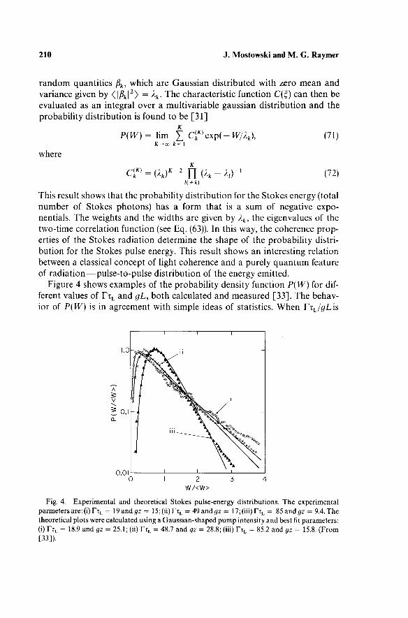
Figure 4 shows examples of the probability density function P(W) for dif-ferent values of T T l and gL, both calculated and measured [33]. The behav-ior of P(W) is in agreement with simple ideas of statistics. When R T L/ g L i s
Fig. 4. Experimental and theoretical Stokes pulse-energy distributions. The experimental p a r m e t e r s a r e : ( i ) r t L = 1 9 a n d 0 z = 15;(ϋ)Γτ^ = 49 and gz = 17;(iii) T T l = 8 5 a n d # z = 9.4. The theoretical plots were calculated using a Gaussian-shaped p u m p intensity and best fit parameters: (i) T T l = 18.9 and gz = 25.1; (ii) T T l - 48.7 and gz = 28.8; (iii) T T l = 85.2 and gz = 15.8. (From [33]).
5. Quantum Statistics in Nonlinear Optics 211
small ( < 1), a single temporal mode is dominant in the Stokes emission (i.e., only one of the kk is large) and P(W) is nearly a negative exponential. In the opposite case, when YxJgL is large ( » 1), many temporal modes are excited. In this case, the Stokes emission is temporally incoherent in the sense that many modes are excited. The distribution P(W) is seen in Fig. 4 to become peaked near the mean value, and to narrow as TxJgL increases.
This behavior of the energy fluctuations can be understood in the following
way. Let be the number of photons emitted in the ith temporal mode. Then,
the detected photon number, or the pulse energy, is the sum of the numbers in
each mode-
rt = nl + n2 + n3 + · · · . (73)
In the limit of many modes, the well-known central limit theorem states that P(W) will be a Gaussian distribution centered at W = (W). The width divided by the mean decreases as the square root of the number of modes excited. The departures from the negative exponential seen in Fig. 4 are indications of the tendency of P(W) to become Gaussian when many modes are excited.
Physically, one may view each coherence time as an independent chance for the molecules to emit a spontaneous photon, which would be amplified to the macroscopic level. In a pure single-mode case, it would be most likely that the atoms do not emit a photon (negative-exponential distribution). As more modes are added, it becomes less likely that all modes will fail to emit a photon (departure from exponential).
Several experiments have been carried out to measure the pulse-energy fluctuations [ 3 3 - 3 6 ] , the earliest being by Walmsley and Raymer [12] and Fabricius et al. [37] . The idea of such measurements is a straightforward one: An ensemble of Ν Stokes pulses is generated by identical pump pulses, and the number of times that the Stokes pulse has an energy within AW of W is determined. As an example, Fig. 4 shows histograms of such measure-ments, showing the transition from transient to steady state [33]. Narrowing of the distribution when the parameter TxL/gz (giving roughly the number of excited temporal modes) increases is clearly seen.
3.7. Temporal Fluctuations
Other quantities exhibit macroscopic fluctuations as well. The present results imply pulse-to-pulse fluctuations of the temporal pulse shapes. This can be seen by replacing, as before, the operators bk by classical random independent quantities ßk, which are Gaussian distributed with variance given by <IAJ
2> = kk. For each pulse, the temporal modes %(x) are excited with a
different set of random amplitudes ßk.

2 1 2 J. Mostowski and M. G. Raymer
This leads to a different and unpredictable pulse shape | £ S ( T , Z ) |2 for each
pulse. Using the mode functions %(τ) and a random number generator to produce
the ft, some typical Stokes pulses have been constructed, and are presented in Fig. 5 [38]. The types of pulses depend on the eignvalues Xk. These eigen-values in turn depend on the value of the parameters T T l and gz. For small Txjgz, a single eigenvalue λχ is dominant, so most of the pulses are structure-less. As Yxjgz increases, higher order eigenvalues become larger, implying more structure on the resulting pulses.
Raymer et al. [38] observed random pulse-to-pulse variation of Stokes pulse shapes. Examples of such pulses, measured with a steak camera, are shown in Fig. 6. While single-peaked shapes were most common, pulses with more complicated structure, corresponding to many excited coherent modes,
Time (ns)
Fig. 5. Theoretical realizations of the random Stokes-pulse intensity. The parameters are: T t l = 80, t l = 5 ns, gz = 30 cm, ζ = 50 cm. The single-peaked pulse shown in (a) is the most common, with the probability of observing pulses with multiple peaks decreasing as the number of peaks increases. (From [38]).

5. Quantum Statistics in Nonlinear Optics 213
0 1 2 0 1 2 Time (ns)
Fig. 6. Examples of the r andom Stokes pulse shapes observed from a Raman generator. The
plots have all been scaled arbitrarily to best illustrate the pulse shapes. The experimental
parameters for all the plots are: T t l — 80, t l = 4.8 ns, gz = 32.6, ζ = 100 cm. These experimental
shapes should be compared with the pulse shapes predicted using the coherent modes theory,
shown in Fig. 5. They were selected from a similar-size statistical sample, and are arranged to show
the similarity. (From [ 3 8 ] ) .
were also seen. These experimentally determined shapes are selected from a statistical sample of size similar to that from which the typical theoretical shapes in Fig. 5 were chosen. The pulses are arranged in the figure to facilitate comparison with Fig. 5.
A closely related quantity exhibiting large pulse-to-pulse fluctuations is the pulse-energy spectrum, studied by MacPherson et al [39].
Summarizing, it has been found that microscopic quantum fluctuations associated with spontaneous Raman scattering can give rise to large fluctua-tions in the total energy and temporal evolution of generated Stokes pulses. This occurs for pulses containing macroscopic amounts (say, \μ], or 10
1 3
photons) of energy. The fluctuations are in great excess of the shot-noise limit.
214 J. Mostowski and M. G. Raymer
4. Q U A N T U M F L U C T U A T I O N S IN O P T I C A L P A R A M E T R I C A M P L I F I C A T I O N
In this section, another class of nonlinear optical effect will be discussed, optical parametric amplification (ΟΡΑ), which arises from three-wave mixing in a nonlinear optical medium. As opposed to the Raman case, the medium is a crystal, which allows for phase matching of the interacting waves. This plays an important role in ΟΡΑ.
One of the waves is the pump (laser) field with high intensity that again will be treated as a given classical field E2, with a central frequency ω2. The two other waves, called idler and signal, are weak and have central frequencies ω, and cos, where ω, + œs = ω2. This condition relates central frequencies of the fields; however, all the waves may have finite bandwidths. The pump pulse is assumed to be transform-limited, so its bandwidth is determined by the pulse duration. The idler and signal waves are dynamical quantities; their band-widths are determined by the interaction. The bandwidths of idler and signal waves are determined primarily by the range of frequencies over which the phase matching can be achieved.
There are many similarities between parametric amplification and SRS. Both processes are three-wave interations; in the Raman case, one of the waves is the material polarization wave, in O P A all three waves are electro-magnetic. In both cases, the weak fields are spontaneously generated from the quantum noise level and are amplified to a macroscopic level during single-pass propagation through the medium. The broad spectrum of the vaccum noise is in both cases filtered by the amplification process. An essential differ-ence between SRS and ΟΡΑ is that SRS is a phase-insensitive amplification process, while O P E is a phase-sensitive amplification process [40].
4.1 . Optical Parametric Amplification
Interaction of the medium with the electromagnetic field in the ΟΡΑ case will be discussed based on a Hamiltonian describing the crystal interacting with the three waves. ΟΡΑ can be most easily achieved in crystals without a center of symmetry; our discussion will be restricted to such crystals.
The energy of the electron in the presence of the field is given by the standard anharmonic model for a non-centrosymmetric crystal [ 4 1 -4 3 ] :
He + Hint = p2/2m + \mœ
2
0x2 + ^ηιξχ
3 - exE. (74)
The interaction energy is of the standard dipole form; the electric field vector Ε is comprised of all the three waves. The resonance frequency of the electronic oscillations ω 0 is different from the driving field frequencies. From this Hamiltonian, the equation of motion for the electron coordinate (either
5. Quantum Statistics in Nonlinear Optics 215
classical or quantum mechanical in the Heisenberg picture) is
3c = -ω2
0χ - ξχ2 + (e/m)E. (75)
We will treat the case that the signal and idler waves are degenerate in center frequency and polarization. The center frequency of both waves is denoted ωι
and the center pump frequency is ω 2 . Introducing the slowly varying compo-nents of the fields Ε and of the electronic coordinates,
E = Σ E\
+ )e'
i{œit-
kiZ) + h.c , (76)
i = 1
χ=Σ x< + )
éTi ( e ,
'f-*>
z ) + h .c , (77)
and assuming phase matching at the carrier frequencies, k2 = 2/c l5 the follow-ing equations for the and x2 components are derived:
x[+) = - / Δ 1 χ
(
1
+ ) - ίζ1χ[~
)χ
{
2
+) + I'MV^, (7 8 a
)
x{
2
+) = -iA2x[
+) - ίξ2χ[
+)2 + ίκ2Ε2
+\ (78b)
where Af = ω 0 — œt are the detunings, assumed large compared to the band-widths of the fields, and ξ ί = ξ/2ω Ι and Kt = e/lœ^.
In the slowly-varying-envelope approximation, the equations for the field amplitudes of the signal and pump are found from the wave equation (16) in Section 2:
c l + l)E[^ = i2neWlx[+\ (79a)
CZ Ct
d d \ c— + — )E2
+) = ΐ2πβω2χ
{
2
+\ (79b)
dz dt J
Equations (78) and (79) need to be solved self-consistently. The fields are weak enough so that they do not cause saturation, and therefore a per-turbative approach is useful. For broad-band fields, this is easier to carry out in the frequency domain. Fourier transforming the equation for x[
+) and
solving to second order in the fields, we find
x x ( v , z ) = Ai - ν
j-< / \ * xdv' Ë\(-v\z) Ë2(v-v\z)
2π Αί-ν' Δ 2 - ( ν - ν ' ) (80)
The frequency argument ν is not the optical frequency, but the difference between the actual frequency and the central frequency ω1 or ω2. The unit of ν is radian/second. Fourier transforming Eq. (79a) and substituting Eq. (80), we find the equation of motion coupling the spectral components of El at ω1 -h ν
216 J. Mostowski and M. G. Raymer
and ωί — ν' with the components of E2 at 2ω χ + ν — ν':
~ ^ ~
c- ίν Εί(ν,ζ) = 2πΐω1Ρ1(ν,ζ)9 (81)
CZ J where the polarization is
Λ(ν,ζ) = ζ^ΜΕ^ν,ζ) + i - fdv'2 ( 2 )(v, v ' )£î(-v' ,z)£ 2(v - ν', z), (82) 2π J
and the susceptibilities are given by
yu>(v) = e Kl ,
(83)
7<*>(v ν') = ~ ^ ' Κ ι Κ2
* y' ' (A t - vKAi - ν ' )(Δ 2 - ν')
The first term in P x is the linear dispersion for the signal wave, and is related to the wave vector by
k(œx + ν) = ^L±lll + 2πχ ( 1 )(ν) ] . c
The second term is nonlinear in the electric fields; it gives the coupling between the polarization and the product of two fields.
In the case of a real crystal, the frequency dependence of the susceptibility is not well-represented by Eq. (83). However, one may generalize the preceding treatment to allow for arbitrary dependence of the susceptibility on the fre-quency by summing over different values of
In real crystals, the dependence of the wavevector k on the frequency is rather weak. Accordingly, the wavevector k(œY + ν) will be expanded in powers of the difference frequency ν up to second order:
k(œx + ν) = k(œx) + vW + \v2k'\ (85)
where
K d ( ° L (86)
The derivative k' is equal to the inverse of the group velocity near the central frequency ω 1 ? while the second derivative k" is related to the group-velocity dispersion (GVD) near this frequency. This approximation takes into account all the relevant physical processes, and simplifies the analysis.

5. Quantum Statistics in Nonlinear Optics 217
The relation between the phase mismatch Ak for the parametric process and the group-velocity dispersion is
Ak(v) = k2 — kl(œ1 + v) — kl(œ1 — ν)
S -k"v2. (87)
Using this expansion, the equation for the signal field becomes
+ 1v
2^Je1(V,Z) = ^dv'f2\v9v')Ë\{-v'9z)Ë2{v - ν', ζ).
(88)
This equation forms the basis for the formal analysis of the ΟΡΑ. A similar equation was found earlier by heuristic arguments [44]. As opposed to the Raman case, this equation does not involve polarization of the medium. This is because the ΟΡΑ is an off-resonance process, and the medium polarization has been eliminated with the help of the adiabatic approximation. However, this equation provides an interesting coupling between the positive- and the negative-frequency parts of the field. This kind of coupling is the source of a large variety of phenomena, both in the classical and quantum descriptions.
Next, the equations for the electric field will be solved. An approximation will be used; namely, it will be assumed that the pump field is monochromatic and unchanged by its interaction in the crystal. Although this approximation neglects possible effects due to quantum fluctuations of the pump [44] , it does not introduce large errors for intense pulses that are long compared to the inverse phase-matching bandwidth, typically 1 0
1 3- 1 0
1 4 rad/s . The frequency
range over which the weak field can be amplified is determined mainly by the phase-matching condition rather than by the bandwidth of the pump field. Thus, the equation becomes [45,46]
_ i(^k' + j v V j j f i ^ z ) = ί ^ χ( 2 )
( ν , v ) Ë \ ( - v 9 z ) E 2 . (89)
The symbol E2 now denotes the electric field strength of the pump, as opposed to the spectral component that appeared in Eq. (88). To solve the problem, we have to specify the equation of motion for the quantity Ë\( — v9Z):
è + I
' ( "v / c
'+
^v
) ^ ( -v
^ ) = -i
v? ( 2 ) (
"v
' "v ) Ê i ( v
'z ) Ê 2
- ( 9 0)
The susceptibility χ( 2 )
(ν , ν) will be approximated by a frequency-independent quantity, and a gain constant will be defined as y = (ω1/ο)χ
(2)Ε2. The solution
of this set of two ordinary linear differential equations is
£ x(v,z) = exp(i/c'vz)[/(v,z)£ 1(v,0) + ig(v9z)Ë\(-v90)l (91a)
£ l ( -v , z ) = exp ( i f c ' vz ) [ / * ( -v , z )£ Î ( -v ,0 ) - ί ^ - ν , ζ ^ ν , Ο ) ] , (91b)
218 J. Mostowski and M. G. Raymer
where the functions / and g are defined as
/ (v , z) = cosh(sz) + i(k"v2/2s) sinh(sz), (92a)
g(v, z) = (y/s) sinh(sz), (92b)
where
5 = V7
2 - (i/c"v2)2. (92c)
Note that ^(v, z) is real, even for imaginary s. These functions obey the property
\f(v,z)\2-\g(v,z)\
2 = l, (93)
which means that Eq. (91b) is a Bogoliubov (squeezing) transformation [47,48]. A similar solution, which is a multimode generalization of the so-called two-mode squeezed states [40], was obtained for the case of the Kerr effect in an optical fiber [49].
The fields in the time domain can now be reconstructed by taking the inverse Fourier transform, which will give temporal convolution of the input field operators at ζ = 0 with the inverse transforms of the / and g functions. We will not reproduce these formulas here, and restrict ourselves to the discussion in the frequency domain.
4.2. Spectrum and Photon Flux of Ο Ρ Α
The spectral density S(v) of the parametrically amplified signal field El is given by the Fourier transform of the two-time field correlation function. For a stationary process, the spectrum is related to the two-frequency correlation function by Eq. (21) with ω, = ω ΐ 9 where the expectation value is calculated in the state of the input signal field, which may be the vacuum |0 > for parametric generation or an arbitrary state for an amplifier. For the generator case, this becomes
<0 |£ î (v , z )£ 1(v ' , z ) | 0> = |^(v, z)| 2< 0 | £ 1( v , 0 )£ Î (v ' , 0)|0>. (94)
The expectation value of the input field that appears on the right-hand side is anti-normally ordered, and is different from zero in the vacuum state. Normally ordered terms give zero, and are not written. The relation between normally ordered fields at the output to anti-normally ordered fields at the input is characteristic of ΟΡΑ. The ant i -normal-ordered expectation in the vacuum state is equal to the commutator, given in Eq. (15b):
<0|Ê 1(v,0)£Î(v',0)|0> = 2π(^ρ^δ(ν - ν'), (95)
where A is, as before, the pump-beam transverse area. Thus, the optical
5. Quantum Statistics in Nonlinear Optics 219
spectrum of El is
S(v) = (l/2n)\g(v,z)\2. (96)
The total photon flux (photons per second) is given by the integral of the spectrum over frequency, Eq. (20):
00
< / > = έ \\s(v,z)\2dv. (97) - o o
The spectrum and the flux will be discussed in the low-gain and high-gain limits. In the low-gain limit (γζ « 1), the spectrum is proportional to
\g(v,z)\2 s (yZ)
2(S i ll (^'2
V
z
2 z ))2 (low gain). (98)
The characteristic width of the spectrum is (in radians/second)
w = J2n/k"z. (99)
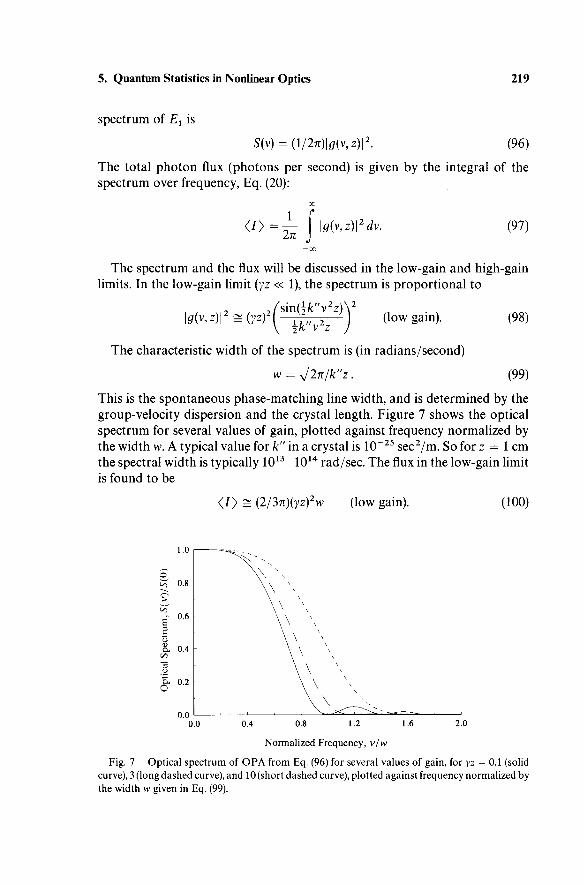
This is the spontaneous phase-matching line width, and is determined by the group-velocity dispersion and the crystal length. Figure 7 shows the optical spectrum for several values of gain, plotted against frequency normalized by the width w. A typical value for k" in a crystal is 1 0 ~ 2 5 sec 2/m. So for ζ = 1 cm the spectral width is typically 1 0 1 3- 1 0 1 4 rad/sec. The flux in the low-gain limit is found to be
</> £ (2/3π)(7ζ)2νν (low gain). (100)
Normalized Frequency, v /w
Fig. 7. Optical spectrum of Ο Ρ Α from Eq. (96) for several values of gain, for y ζ = 0.1 (solid curve), 3 (long dashed curve), and 10 (short dashed curve), plotted against frequency normalized by the width w given in Eq. (99).
2 2 0 J. Mostowski and M. G. Raymer
The high-gain limit is reached when y ζ » 1. In this case, the spectrum is proportional to
\g(v,z)\2 * i e x p ( 2 y z ) e x p [ - ( v / 5 )4] (high gain), (101)
where the width is now
b = lyz/π2] 1 / 4w - [4y / ( / c" ) 2 z ] 1 / 4 (102)
The dependence of the high-gain spectrum on the frequency resembles to some extent the corresponding result for the Raman case, Eq. (62). However, we get a v
4 dependence in the exponent rather than v
2. For fixed w, increasing the gain
coefficient y leads to broadening of the spectrum, in contrast to the case in SRS where narrowing occurs. This broadening occurs because in high gain the phase matching is enforced only within a gain length y ~
l.
The flux of the signal in the high-gain limit can be calculated by integrating the spectrum over frequencies. We find (using the gamma function)
</> Ξ 0.9(ft/47ü)exp(2yz). (103)
Note that the flux grows slightly slower than exponentially in ζ due to the dependence of b on z
1 / 4. This is similar to the ζ
1 /2 factor appearing in SRS
(Eq. (59)). In both cases, these factors arise from the dependence of the band-width on the medium length.
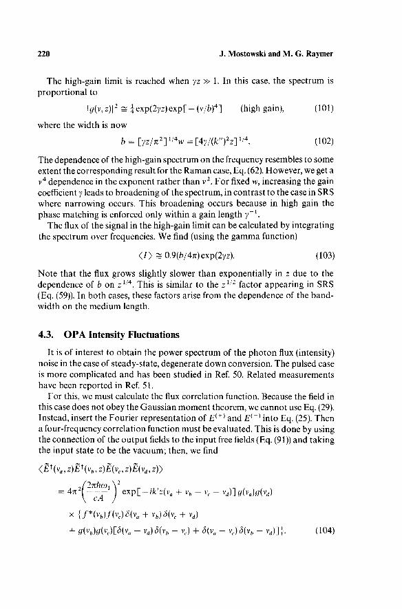
4.3. Ο Ρ Α Intensity Fluctuations
It is of interest to obtain the power spectrum of the photon flux (intensity) noise in the case of steady-state, degenerate down conversion. The pulsed case is more complicated and has been studied in Ref. 50. Related measurements have been reported in Ref. 51.
For this, we must calculate the flux correlation function. Because the field in this case does not obey the Gaussian moment theorem, we cannot use Eq. (29). Instead, insert the Fourier representation of E
i + ) and E
{~
) into Eq. (25). Then
a four-frequency correlation function must be evaluated. This is done by using the connection of the output fields to the input free fields (Eq. (91)) and taking the input state to be the vacuum; then, we find
(fr(va,z)ËHvb,z)Ë(vc,z)Ë(vd,z))
= A n 2 i ~ ~ J ^ j exp[-ifc 'z(v e + vb - vc - vd)]g(va)g(vd)
x {f*(vb)f(vc)S(va + vb)ö(vc + vd)
+ g(vb)g(vc)LÔ(va - vd)ô(vb - vc) + δ(να - vc)ô(vb - v d)]}. (104)
5. Quantum Statistics in Nonlinear Optics 221
Using this function and evaluating the necessary integrals with help of the delta functions gives the result for the power spectrum of the photon flux noise:
00
Γ dv'
P(v) = </>+ I _ [ | 0 ( v ' , z ) |2| 0 ( v - v ' , z ) |
2
- o o
+ g*(v\z)f*(v'9 z)g(v - v', z)f(v - v', z)], (105)
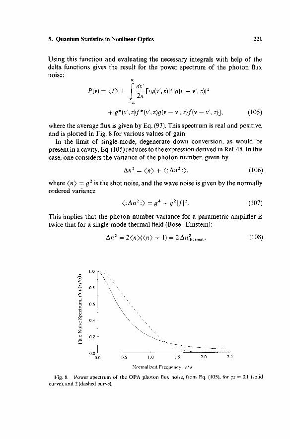
where the average flux is given by Eq. (97). This spectrum is real and positive, and is plotted in Fig. 8 for various values of gain.
In the limit of single-mode, degenerate down conversion, as would be present in a cavity, Eq. (105) reduces to the expression derived in Ref. 48. In this case, one considers the variance of the photon number, given by
An2 = <n> + <:Δπ
2:> , (106)
where <n> = g2 is the shot noise, and the wave noise is given by the normally
ordered variance
<.:An2:y=g
4 + g
2\f\
2. (107)
This implies that the photon number variance for a parametric amplifier is twice that for a single-mode thermal field (Bose-Einstein):
An2 = 2<n>«n> + 1) = 2 A n t
2
h e r m a l. (108)
Normalized Frequency, v/w
Fig. 8. Power spectrum of the Ο Ρ Α photon flux noise, from Eq. (105), for y ζ = 0.1 (solid
curve), and 2 (dashed curve).
222 J. Mostowski and M. G. Raymer
4.4. Noise Reduction and Squeezing
In spite of the fact that the photon flux in parametric down conversion exhibits very large fluctuations (even larger than thermal), some other mea-surable quantities have greatly reduced noise. This noise reduction can go not only below the thermal level, but also below the standard shot-noise level. This possibility arises from the correlations between the fluctuations at different frequencies, not present in thermal nor in coherent light, and makes parametric amplification a paradigm for a newly understood class of processes referred to as two-photon quantum optics [40]. The correlations at different frequencies result from the simultaneous creation of pairs of photons at frequencies symmetrically displaced from one half of the pump frequency.
The states of the field generated by the parametric amplifier are a special class of states that exhibit noise reduction [52], and are usually refered to as squeezed states. Alternative methods of generating the squeezed states involve four-wave mixing in atomic vapors [10] or optical fibers [53], resonance fluorescence by atoms in an optical cavity [54], and, in the microwave region, by wave mixing in a Josephson junction [55] . Extensive discussion and references are given in Ref. 11.
It is customary to discuss the quantum fluctuations of the field in terms of the creation and annihilation operators a
f(v, z) and α(ν,ζ), respectively, asso-
ciated with each frequency, which for narrow-band fields are connected to the frequency-domain field operators by
These are defined so that, using the field commutator equation ( 15b), they obey
In the case that only one mode is excited (as in a cavity), the creation and annihilation operators are defined in the usual way [6] , so that [ a , a
f] = 1.
This case will be reviewed briefly. (See Ref. 14 for a fuller discussion.) New dimensionless quadrature operators, formally analogous to position and mo-mentum operators, are then defined by
(109)
[α(ν,ζ), ατ(ν ' ,ζ ) ] = δ(ν — ν'). (110)
(111)
5. Quantum Statistics in Nonlinear Optics 223
where j? is a reference phase, defined relative to some time origin in the problem. This implies that the standard deviations obey the uncertainty relation
AX AY > | . (112)
The case of a coherent state (which could be the vacuum) is distinguished by the property that each quadrature has the same uncertainty, and the product equals the minimum possible value:
AXCoh = AYCoh = I (113)
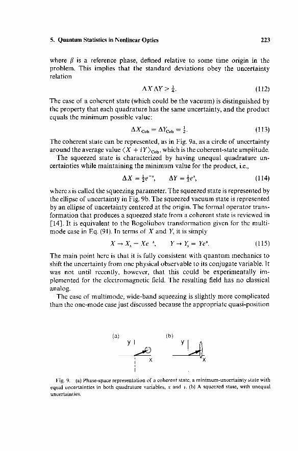
The coherent state can be represented, as in Fig. 9a, as a circle of uncertainty around the average value <X + * ^ > c o h > which is the coherent-state amplitude.
The squeezed state is characterized by having unequal quadrature un-certainties while maintaining the minimum value for the product, i.e.,
AX = \e~\ AY = \e\ (114)
where s is called the squeezing parameter. The squeezed state is represented by the ellipse of uncertainty in Fig. 9b. The squeezed vacuum state is represented by an ellipse of uncertainty centered at the origin. The formal operator trans-formation that produces a squeezed state from a coherent state is reviewed in [14]. It is equivalent to the Bogoliubov transformation given for the multi-mode case in Eq. (91). In terms of X and Y, it is simply
X^Xs = Xe~\ Y-+Ys=Yes. (115)
The main point here is that it is fully consistent with quantum mechanics to shift the uncertainty from one physical observable to its conjugate variable. It was not until recently, however, that this could be experimentally im-plemented for the electromagnetic field. The resulting field has no classical analog.
The case of multimode, wide-band squeezing is slightly more complicated than the one-mode case just discussed because the appropriate quasi-position
(a) (b)
Fig. 9. (a) Phase-space representation of a coherent state, a minimum-uncertainty state with
equal uncertainties in both quadra ture variables, χ and y. (b) A squeezed state, with unequal
uncertainties.
2 2 4 J. Mostowski and M. G. Raymer
and momentum operators involve creation and annihilation operators at more than one frequency [40] :
X(v,z) = X
-[a{v9z)e~iß + a\-v9z)e
iß\
(116)
Υ(ν,ζ) = l [ f l ( v , z ) é r * - a\-v9z)eiß\
2ι
This definition reflects the correlations that exist between the frequencies displaced by + ν from the central frequency (ωι in down conversion). Note that here X and Y are not Hermitian. To show that these are the proper variables to describe squeezing, we reexpress the solutions for down conver-sion, Eq. (91), using Eq. (109), as
where
X(v9z) = fxx(v9z)X(v90) + fxy(v,z)Y{v90)9
Y(v,z) = fyx(v9z)X(v90) + fyy(v,z)Y(v90)9
/ „ (v , z ) = ^ R c F _ ( v ) ,
fxy(v9z) = eikvz
lmF_(v)9
fyx(v9z) = ieik'^lmF+(v)9
fyy(v9z) = ieih'*
zReF+(v)9
(117)
(118)
and
F±(v) = cosh(sz) + (i/s){^k"v2 ± ye~
i2ß) sinh(sz). (119)
The important point to note about this solution is that for each value of frequency v, the squeezing occurs along a different axis in phase space; i.e., a different value of β minimizes the noise variance in the X variable. In the high-gain limit (sz » 1), this value is that which minimizes fxx, and is found to be determined by
s in2ß = s/y9 cos2i8 = \k"v2/y. (120)
Observe that at exact degeneracy (v = 0), maximum squeezing occurs at the phase value β = π/4. Then, Eq. (117) becomes
X(v9z) = e~yzX(v90)9 Y(v9z) = e
y z7(v,0) , (121)
which is of the same form as the single-mode behavior, Eq. (115). For frequencies ν other than zero, dispersion is present and maximum squeezing occurs at a phase other than π/4. For frequencies near zero, maximum squeez-ing occurs at approximately β ^ π/4 — k"v
2/4y.
5. Quantum Statistics in Nonlinear Optics 225
4.5. Homodyne Detection of Field-Quadrature Noise
The physical quantities that can display reduced noise are the quadrature amplitudes of the electric field. The electric field is not easy to measure directly since it oscillates at an optical frequency, too fast to be detected by any macroscopic device. It is usually flux or another correlation function of the electric field that is measured. The flux of an optical field varies on a much slower time scale, and can be measured by means of the photoelectric effect.
Homodyne detection is used in order to measure indirectly the electric-field quadrature amplitudes of light [56] . Homodyning reduces the measurement of a rapidly oscillating field to the measurement of slowly varying intensities. In the case of optical fields, homodyning is accomplished by adding a strong coherent field to the signal field that is to be measured. The coherent field, called the local oscillator, is monochromatic; its frequency is equal to the cen-tral frequency ωγ of the signal field. What is measured is the photon flux of the sum field, called the homodyne field, from which the quadrature ampli-tudes can be deduced.
The quadrature amplitudes Ec and Es are hermitian operators defined by
EG(t,z) = Ei +
%z)e~ia + E
{~%z)e\
(122) E,(t,z) = - i [ F
( + )( i , z ) e -
i a - £<->(t,z)e
t e],
where ALOe~i<x is the complex amplitude of the coherent state with phase α
describing the local oscillator field. The amplitude ALO is assumed to be much larger than that of the signal field. The electric field of the signal (oscillating at optical frequency) is, at ζ = 0,
Ei+)(t9z)e~
it0it + E
{-\t,z)e
i(0it = Ec(t,z)œs(œlt - α) + £ s( i , z )s inKi - α).
(123)
The amplitude Ec is in phase with the local oscillator while the amplitude Es is
90° out of phase. The linear superposition of the two fields is achieved using a beamsplitter
with complex reflectivity and transmisivity r and i, respectively. The detector placed in one of the outputs of the beamsplitter measures the flux of the homodyne field
£< + >(*, z) = rEi + )
(t,z) + M L Oé Tf a
. (124)
To lowest order in the signal field, the homodyne flux is
/«(*) = 2 ^{ | ί | 2
^ ° +
N^Lo[cos(rç)F c - sin(i7)£e]}, (125)
where the phase η is associated with the beamsplitter, ir* = \tr\e~in. Thus,
fluctuations of the quadrature amplitudes are manifested as noise on the homodyne flux.
2 2 6 J. Mostowski and M. G. Raymer
The photon flux equation (125) corresponding to the homodyne field can be spectrally analyzed by calculating the Fourier transform of its autocorrelation function as in Eq. (22), to give the homodyne noise spectrum PH(v) in terms of the homodyne flux correlation function C H( T ) [19,20,57,58]. The correlation function, to lowest order in the weak signal field, is found by putting the homodyne field (124) into Eq. (25), giving
cA ^(τ) = <ΙΗ}δ(τ) + ^^\»\
2<^ο>
χ [<£<->(i,z)E( + )
(t + τ, z)> + <E{~\t + τ, ζ )£
( + )(ί,ζ)>
+ e~2iitl + a
\TEi-
)(t9z)E
{-
)(t + τ, z)>
+ β2ί<"
+ "><7Έ
( + )(ί + τ, ζ )£
( + )( ί ,ζ)>], (126)
where the local oscillator flux is < / L O> = (cA/2nhœ1)Al0 and the homodyne flux is approximated as < / H > = <^LO>- Putting this correlation function into Eq. (22) gives the general expression for the rf homodyne spectrum. Often, as for coherent or thermal light, the signal correlation functions < F
( _ )F
( _ )> and
< £( + )
F( + )
> are zero. This is not the case, however, in down conversion, due to the correlations between frequency components at ± v.
For the case of light generated by parametric down conversion, the needed correlation functions are found from the solutions in the frequency domain, Eq. (91). The rf homodyne spectrum is then found to be
W = | t | 2</ Lo> + M2< / L O > W ( V ) , (127)
where
W(v) = 2{[#(v ,z) ]2 - | / (v,z) |^(v,z)sin[2a + 2η + 0(v)]} (128)
where φ(ν) is the phase of / (v , z), given in Eq. (92), and depends on frequency. A similar result was obtained for the case of the Kerr effect in an optical fiber [59,60] as well as ΟΡΑ as treated here [45,46] . The first term in PH(v) is the shot noise associated with the local oscillator transmitted by the beamsplitter and incident on the detector. It is white noise, that is, constant for all rf frequencies. The second term is the change of the noise due to the interference with the parametric signal. The quantity W(y) has a lower bound of — 1 and no upper bound. The lower bound is approached when the parametric down-conversion gain is large and the phase is adjusted to satisfy 2α + 2η + φ = π/2.
It can be seen that the homodyne flux is the quantity that can have noise either greater or less than the standard shot-noise limit at rf frequency v. By adjusting the parameters, one may produce a light field with essentially no fluctuations in the photon flux. The beamsplitter reflectivity should be
5. Quantum Statistics in Nonlinear Optics 227
nearly unity. The local oscillator should be strong enough so that even after attenuation by the beamsplitter it dominates the parametric signal at the detector. Also, the phase at this frequency must be adjusted to π/2. In practice, the value of η is usually varied by slight movement of the beamsplitter. If, for some choice of phase, the homodyne field has noise less than the standard shot-noise level, the down-conversion field is said to be squeezed.
In the high-gain limit (sz » 1), the phase of | / (v ,z) | is given by
cos[>/2 - φ(ν,ζ)] = sin[(/>(v,z)] s i/c"v2/y, (129)
which means that the value of 2α + 2η that gives the greatest noise reduction satisfies
cos[2a + 2rç] = \k"v2/y. (130)
Comparing this with Eq. (120) shows that we can identify the reference phase denoted by β in Section 4.4 as being equal to β = a. + 77, that is, the phase of the local oscillator modified by the beamsplitter. Equation (130) shows that each rf frequency requires a different local-oscillator phase to maximize the noise reduction at that frequency.
The homodyne spectrum. Eq. (127), is plotted versus frequency in Fig. 10 for 2a + 2rç = π/2, which maximizes the noise reduction at ν = 0. For this choice of phase, W(v) can be approximated in the high-gain limit as
W(v)^ - 1 + 2 { 1 -cos[( />(v,z)]} | / (v ,z) |2. (131)
The noise-reduction bandwidth can be defined as that rf frequency v N R at which W(v) = —1/2. This is, in the high-gain limit,
vtn = (2^27/k")l,2e-"'2. (132)
For large gain, the noise-reduction bandwidth is smaller than the down-conversion optical bandwidth b in Eq. (102). For example, for y ζ = 5 and typical crystal parameters given in Section 4.2, v N R is about 15% of b, which is about 1 0
1 3- 1 0
1 4 rad/sec.
4.6. Experimental Realization of Photon Noise Reduction by
Traveling-Wave Parametric Amplification
The first observation of quadrature-squeezed light utilized four-wave mix-ing near an atomic resonance in a cavity [10], as proposed by Yuen and Shapiro [61]. This method is limited by the presence of spontaneous-emission noise, which degrades the delicate correlations that occur between frequency components of the field. Using nonresonant nonlinearities, such as para-metric amplification in crystals or Kerr effect in optical fibers, avoids this spontaneous-emission noise and allows larger degrees of squeezing to be
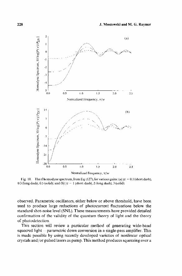
228 J. Mostowski and M. G. Raymer
2 - i 7
" " /
OH /
-3 - / G / >, /
7 3 - 4 /
Ο 4
^ / Β " ο
Χ .5 I , , , , , 0.0 0.5 1.0 1.5 2.0 2.5
Normalized Frequency, V/w
I / / G- _14 - / &o y
G / >Ï /
ο -21 - /
ε / ^ _28 I • ' • ' • 1 • ' • 1
0.0 0.5 1.0 1.5 2.0 2.5
Normalized Frequency, v/w
Fig. 10. The r fhomodyne spectrum, from Eq. (127), for various gains: (a) yz — 0.1 (short dash), 0.3 (long dash), 0.5 (solid); and (b) yz = 1 (short dash), 2 (long dash), 3 (solid).
observed. Parametric oscillators, either below or above threshold, have been used to produce large reductions of photocurrent fluctuations below the standard shot-noise level (SNL). These measurements have provided detailed confirmation of the validity of the quantum theory of light and the theory of photodetection.
This section will review a particular method of generating wide-band squeezed light—parametric down conversion in a single-pass amplifier. This is made possible by using recently developed varieties of nonlinear optical crystals and/or pulsed lasers as pump. This method produces squeezing over a
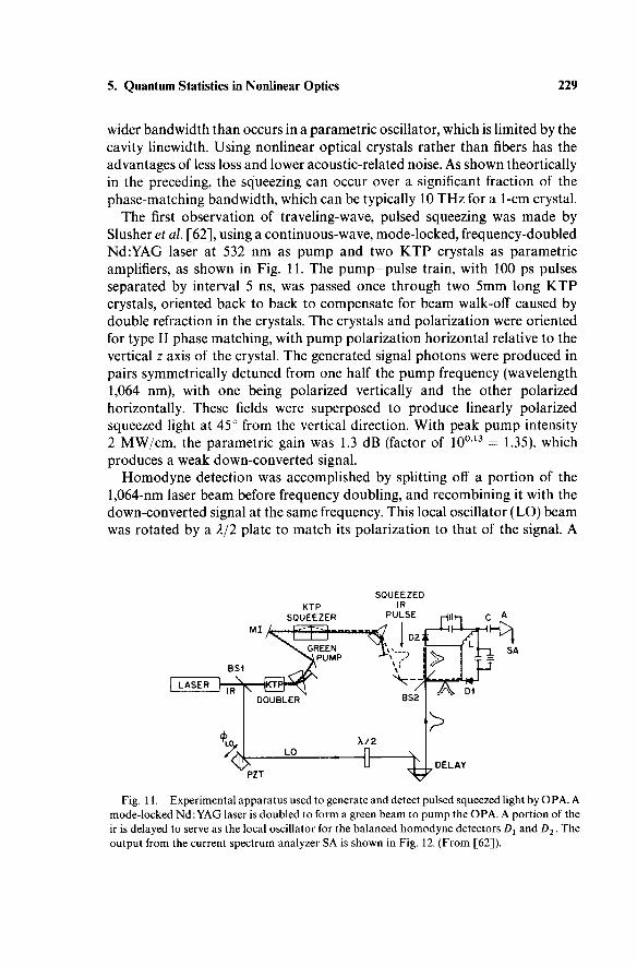
5. Quantum Statistics in Nonlinear Optics 2 2 9
wider bandwidth than occurs in a parametric oscillator, which is limited by the cavity linewidth. Using nonlinear optical crystals rather than fibers has the advantages of less loss and lower acoustic-related noise. As shown theortically in the preceding, the squeezing can occur over a significant fraction of the phase-matching bandwidth, which can be typically 10 THz for a 1-cm crystal.
The first observation of traveling-wave, pulsed squeezing was made by Slusher et al. [62], using a continuous-wave, mode-locked, frequency-doubled Nd:YAG laser at 532 nm as pump and two K T P crystals as parametric amplifiers, as shown in Fig. 11. The pump-pu l se train, with 100 ps pulses separated by interval 5 ns, was passed once through two 5mm long K T P crystals, oriented back to back to compensate for beam walk-off caused by double refraction in the crystals. The crystals and polarization were oriented for type II phase matching, with pump polarization horizontal relative to the vertical ζ axis of the crystal. The generated signal photons were produced in pairs symmetrically detuned from one half the pump frequency (wavelength 1,064 nm), with one being polarized vertically and the other polarized horizontally. These fields were superposed to produce linearly polarized squeezed light at 45° from the vertical direction. With peak pump intensity 2 MW/cm, the parametric gain was 1.3 dB (factor of 1 0
0 13 = 1.35), which
produces a weak down-converted signal.
Homodyne detection was accomplished by splitting off a portion of the 1,064-nm laser beam before frequency doubling, and recombining it with the down-converted signal at the same frequency. This local oscillator (LO) beam was rotated by a λ/2 plate to match its polarization to that of the signal. A
SQUEEZED KTP IR
Fig. 11. Experimental appara tus used to generate and detect pulsed squeezed light by Ο Ρ Α . A mode-locked N d : YAG laser is doubled to form a green beam to p u m p the Ο Ρ Α . A port ion of the ir is delayed to serve as the local oscillator for the balanced homodyne detectors D{ and D2. The output from the current spectrum analyzer SA is shown in Fig. 12. (From [62]).
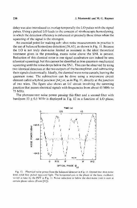
230 J. Mostowski and M. G. Raymer
delay was also introduced to overlap temporally the LO pulses with the signal pulses. Using a pulsed LO leads to the concept of stroboscopic homodyning, in which the detection efficiency is enhanced at precisely those times when the squeezing of the signal is the strongest.
An essential point for making sub-shot-noise measurements in practice is the use of balanced homodyne detection [56,63], as shown in Fig. 11. Because the LO is not truly shot-noise limited as assumed in the ideal theoretical treatment given in the preceding, excess noise above the SNL is present. Reduction of this classical noise in one signal quadrature can indeed be seen (classical squeezing), but this cannot be identified as true quantum-mechanical squeezing until the noise drops below the SNL. This can be observed by using two identical detectors at the two outputs of the beamsplitter, and subtracting their signals electronically. Ideally, the classical wave noise cancels, leaving the quantum noise. The subtraction can be done using a microwave circuit element called a hybrid junction [64] or, as in Fig. 11, directly at the junction of two wires. The figure also shows an LC circuit involving the summing junction that passes electrical signals with frequencies from about 45 MHz to 75 MHz.
The photocurrent noise power passing this filter and a second filter with bandpass 53 ± 0.5 MHz is displayed in Fig. 12 as a function of LO phase,
time (s) 0.5 1.0
Ε m
(Τ
ο
ο
-
A A-Λ / χ A A-Λ / χ 63.5 -\ / ' ' ι / t
I
- Ι
f ί * ! 1. ! y ι: ι \ J :
- 6 4 1-4 ι II / I ί
1,
ί '
I
ί Ί
6 4 5
I I ι -Γ \ ι -7772 7Γ 7Γ/2
OPTICAL PHASE ψ L0
Fig. 12. Electrical noise power from the balanced detector in Fig. 11. Dotted line: shot-noise
level; solid line: pulsed squeezed light. The horizontal axis is the phase of the local oscillator,
varied in time by the P Z T in Fig. 11. Noise reduction to below the shot-noise limit is seen at
certain phase values. (From [62]).

5. Quantum Statistics in Nonlinear Optics 231
which is controlled by slowly moving a mirror with a piezoelectric translator (PZT in Fig. 11). The dotted line at - 64 dBm is the SNL of the LO, obtained by blocking the down-converted signal beam. The solid line shows the noise in the difference signal with the signal beam unblocked—at certain values of the LO phase, the noise drops below the SNL.
A physical interpretation of this result is that the two beams striking the detectors are "twin" photon beams, i.e., are exact copies of one another. So each time a photon strikes one detector, a companion photon strikes the other detector. It is thus clear that it is necessary to have a high quantum efficiency for the detectors to convert each photon into an electron. Otherwise, decor-relation of the signals would occur, and the intrisically quantum features of the light field would not be seen. A noise no lower than the SNL would be obtained. The detectors used are typically solid-state photodiodes (such as InGaAs) operated at room temperature with quantum efficiency around 90%. Another important factor is the homodyne efficiency, which depends on the spatial overlap of the signal mode u(r) and the LO mode uLO(r) at the detector surface [64] :
If this factor is much less than unity, sub-SNL detection will not occur. With care, this quantity can be made greater than 90% [64].
Although the maximum amount of noise reduction shown in Fig. 12 is 0.6 dB below the SNL, somewhat greater noise reductions have been observed. Hirano and Matsuoka, using a similar set-up as in Fig. 11, but using a more efficient down-conversion crystal, B a 2 N a N b 5 0 1 5, observed a 1.1 dB reduction from about 1 MHz to 70 MHz [65] . At the present time, the largest quadra-ture squeezing has been obtained by parametric oscillation in a cavity, where the noise was reduced by a factor of two (3 dB) below the SNL [64].
The previously discussed experiments [62,65] used cw, mode-locked lasers to pump the down conversion. Consequently, the signal produced was mod-ulated at the mode-locking repetition rate (200 MHz in [62]). This created strong rf components in the homodyne spectrum at this modulation frequency and its harmonics, which were difficult to subtract accurately, and so prevented sub-SNL detection within about 1 MHz of these frequencies. By using single-pulse, Q-switched lasers with repetition rates in the 10 kHz range, these un-wanted noise spikes can be moved to much lower frequencies, in principle leaving the entire spectral region above about one megahertz with noise less than the SNL. Using such a laser, Kumar et al [66] observed 0.8 dB reduction below the SNL using a set-up similar to that in Fig. 11. These authors also pointed out the interesting fact that a multimode, non-phase-locked, pulsed laser could be used to generate squeezed light by down conversion. Using
η = utQ{r)u{r)d2r . (133)
232 J. Mostowski and M. G. Raymer
arguments concerning temporal modes, analogous to the discussion in Sec-tion 3.5 for SRS, they pointed out that the homodyne technique measures the operator [67,68].
where </>LO(0 is the time-dependent L O field and Ei+)(t) is the signal-field
operator. This integral is the temporal analog to that in Eq. (133) for the spatial overlap efficiency. Thus, by properly choosing the LO field </>LO(0> a certain time evolution of the signal field can be projected out and measured. Kumar et al found that by using a portion of the multimode pump pulse before fre-quency doubling as the LO, as in Fig. 11, the part of the signal field that is squeezed is projected out and measured. This produced sub-SNL detection even though the LO field changed on every laser shot due to random phases between longitudinal laser modes. In this sense, they generated and detected squeezing using an incoherent pump field.
Acknowledgments
We wish to thank J. Cooper for helpful comments on parts of the manu-script and S. Yang for preparing several of the figures. This work was sup-ported by the U.S. National Science Foundat ion and the U.S. Army Research Office. J. M. wishes to acknowledge a JILA Visiting Fellowship.
References
1. J. C. MacGillivray and M. S. Feld, Phys. Rev. A 14, 1169 (1976). 2. R. Glauber and F. Haake , Phys. Lett. 68A, 29 (1978). 3. M. F. H. Schuurmans and D. Polder, Phys. Lett. 72A, 306 (1979). 4. F. A. Hopf, Phys. Rev. A 20, 2064 (1979). 5. I. Bialynicki-Birula and Z. Bialynicki-Birula, " Q u a n t u m Electrodynamics," Pergamon,
Oxford, 1975. 6. R. Loudon, "The Q u a n t u m Theory of Light," Clarendon Press, Oxford, 1983. 7. C. Cohen-Tannoudji , J. Dupont -Roc , and G. Grynberg, "Pho tons and Atoms," Wiley
(Interscience), New York, 1989. 8. C. M. Caves, Phys. Rev. D 26, 1817 (1982). 9. C. K. Hong and L. Mandel , Phys. Rev. Lett. 56, 58 (1986).
10. R. E. Slusher, L. W. Hollberg, Β. Yurke, J. C. Mertz, and J. F. Valley, Phys. Rev. Lett. 55,2409 (1985).
11. H. J. Kimble and D. F. Walls, eds., J. Opt. Soc. Am. Β 4 , 1450-1741 (1987). 12. I. A. Walmsley and M. G. Raymer, Phys. Rev. Lett. 50, 962 (1983). 13. M. G. Raymer, K. Rzazewski, and J. Mostowski , Opt. Lett. 7, 71 (1982). 14. R. Loudon and P. L. Knight, J. Mod. Phys. 34, 709 (1987). 15. M. C. Teich and B. Saleh, Quantum Opt. 1, 153 (1989). 16. D. F. Walls, Nature 306, 141 (1983).
(134)
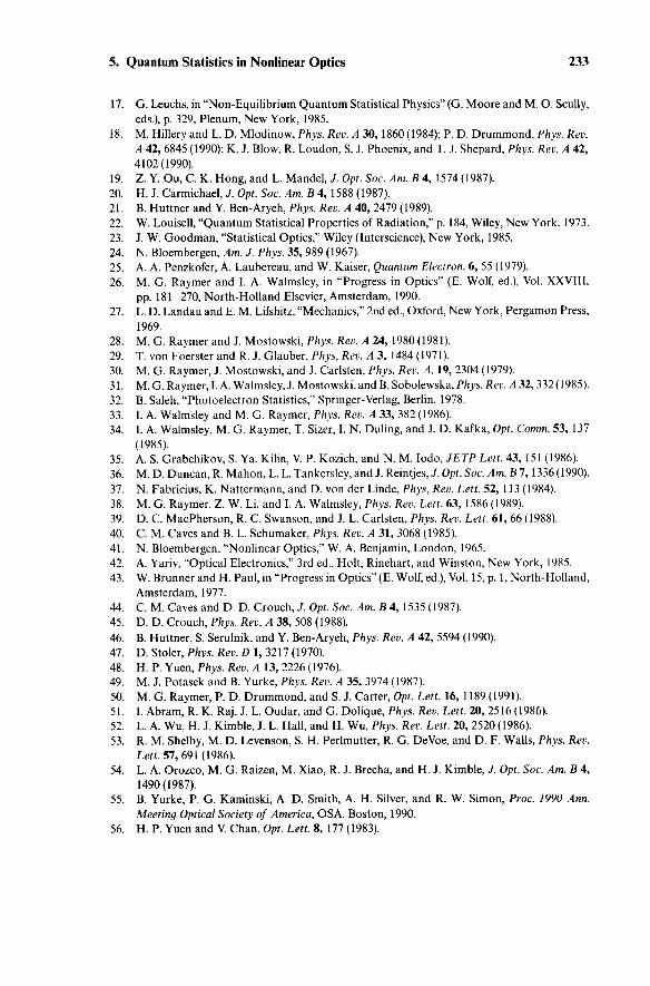
5. Quantum Statistics in Nonlinear Optics 233
17. G. Leuchs, in "Non-Equi l ibr ium Q u a n t u m Statistical Physics" (G. Moore and M. O. Scully,
eds.), p. 329, Plenum, New York, 1985.
18. M. Hillery and L. D . Mlodinow, Phys. Rev. A 30 ,1860 (1984); P. D. D r u m m o n d , Phys. Rev.
A 42, 6845 (1990); K. J. Blow, R. Loudon, S. J. Phoenix, and T. J. Shepard, Phys. Rev. A 42,
4102(1990).
19. Z. Y. Ou, C. K. Hong, and L. Mandel , J. Opt. Soc. Am. Β 4, 1574 (1987).
20. Η. J. Carmichael, J. Opt. Soc. Am. Β 4, 1588 (1987).
21. Β. Hut tner and Y. Ben-Aryeh, Phys. Rev. A 40, 2479 (1989).
22. W. Louisell, " Q u a n t u m Statistical Properties of Radiation," p. 184, Wiley, New York. 1973.
23. J. W. G o o d m a n , "Statistical Optics," Wiley (Interscience), New York, 1985.
24. N. Bloembergen, Am. J. Phys. 35, 989 (1967).
25. A. A. Penzkofer, A. Laubereau, and W. Kaiser, Quantum Electron. 6, 55 (1979).
26. M. G. Raymer and I. A. Walmsley, in "Progress in Opt ics" (E. Wolf, ed.), Vol. XXVIII,
pp. 181-270, Nor th-Hol land Elsevier, Amsterdam, 1990.
27. L. D. Landau and Ε. M. Lifshitz, "Mechanics," 2nd ed., Oxford, New York, Pergamon Press,
1969.
28. M. G. Raymer and J. Mostowski , Phys. Rev. A 24, 1980 (1981).
29. T. von Foerster and R. J. Glauber, Phys, Rev. A 3 , 1484 (1971).
30. M. G. Raymer, J. Mostowski , and J. Carlsten, Phys. Rev. A. 19, 2304 (1979).
31. M. G. Raymer, I. A. Walmsley, J. Mostowski , and B. Sobolewska, Phys. Rev. A 32,332 (1985).
32. B. Saleh, "Photoelectron Statistics," Springer-Verlag, Berlin, 1978.
33. I. A. Walmsley and M. G. Raymer, Phys. Rev. A 33 , 382 (1986).
34. I. A. Walmsley, M. G. Raymer, T. Sizer, I. N. Duling, and J. D. Kafka, Opt. Comm. 53, 137
(1985).
35. A. S. Grabchikov, S. Ya. Kilin, V. P. Kozich, and Ν. M. Iodo, JETP Lett. 43 , 151 (1986).
36. M. D. Duncan, R. Mahon , L. L. Tankersley, and J. Reintjes, J. Opt. Soc. Am. Β 7, 1336 (1990).
37. Ν. Fabricius, Κ. Na t te rmann , and D. von der Linde, Phys, Rev. Lett. 52, 113 (1984).
38. M. G. Raymer, Z. W. Li, and I. A. Walmsley, Phys. Rev. Lett. 63, 1586 (1989).
39. D. C. MacPherson, R. C. Swanson, and J. L. Carlsten, Phys. Rev. Lett. 6 1 , 66 (1988).
40. C. M. Caves and B. L. Schumaker, Phys. Rev. A 3 1 , 3068 (1985).
41. N . Bloembergen, "Nonlinear Optics," W. A. Benjamin, London, 1965.
42. A. Yariv, "Optical Electronics," 3rd ed., Holt , Rinehart, and Winston, New York, 1985.
43. W. Brunner and H. Paul, in "Progress in Opt ics" (E. Wolf, ed.), Vol. 15, p. 1, Nor th-Hol land,
Amsterdam, 1977.
44. C. M. Caves and D. D. Crouch, J. Opt. Soc. Am. B 4, 1535 (1987).
45. D. D. Crouch, Phys. Rev. A 38, 508 (1988).
46. B. Huttner , S. Serulnik, and Y. Ben-Aryeh, Phys. Rev. A 42, 5594 (1990).
47. D . Stoler, Phys. Rev. D 1, 3217 (1970).
48. H. P. Yuen, Phys. Rev. A 13, 2226 (1976).
49. M. J. Potasek and B. Yurke, Phys. Rev. A 35, 3974 (1987).
50. M. G. Raymer, P. D. D r u m m o n d , and S. J. Carter, Opt. Lett. 16, 1189 (1991).
51. I. Abram, R. K. Raj, J. L. Oudar , and G. Dolique, Phys. Rev. Lett. 20, 2516 (1986).
52. L. A. Wu, H. J. Kimble, J. L. Hall, and H. Wu, Phys. Rev. Lett. 20, 2520 (1986).
53. R. M. Shelby, M. D. Levenson, S. H. Perlmutter , R. G. DeVoe, and D. F. Walls, Phys. Rev.
Lett. 57, 691 (1986).
54. L. A. Orozco, M. G. Raizen, M. Xiao, R. J. Brecha, and H. J. Kimble, J. Opt. Soc. Am. B 4,
1490(1987).
55. B. Yurke, P. G. Kaminski , A. D. Smith, A. H. Silver, and R. W. Simon, Proc. 1990 Ann.
Meeting Optical Society of America, OSA, Boston, 1990.
56. H. P. Yuen and V. Chan, Opt. Lett. 8, 177 (1983).
234 J. Mostowski and M. G. Raymer
57. M. Collet and C. W. Gardiner , Phys. Rev. A 3 1 , 3761 (1985). 58. M. Collet and D. F. Walls, Phys. Rev. A 32, 2887 (1985). 59. M. J. Potasek and B. Yurke, Phys. Rev. A 35, 3974 (1987). 60. P. D. D r u m m o n d and S. J. Carter, J. Opt. Soc. Am. Β 4, 1565 (1987). 61. H. P. Yuen and J. H. Shapiro, Opt. Lett. 4, 334 (1979). 62. R. E. Slusher, P. Grangier, A. La Porta , B. Yurke, and M. J. Potasek, Phys. Rev. Lett. 59,2566
(1987). 63. B. L. Schumaker, Opt. Lett. 9, 189 (1984). 64. L. A. Wu, M. Xiao, and H. J. Kimble, J. Opt. Soc. Am. Β 4, 1465 (1987). 65. T. Hirano and M. Matsuoka , Opt. Lett. 15, 1153 (1990). 66. P. Kumar , O. Aytur, and J. Huang, Phys. Rev. Lett. 64, 1015 (1990). 67. H. P. Yuen and J. H. Shapiro, IEEE Trans. Inf. Theory 26, 78 (1980). 68. P. D. Drummond , S. J. Carter, and R. M. Shelby, Opt. Lett. 14, 373 (1989).