arX

iv:h

ep-t

h/01

0609

4 v2

9

Feb

2005

Quantum superfield supersymmetryA.Yu. Petrov

Departamento de Fisica e Matematica,

Instituto de Fisica,

Universidade de Sao Paulo,

Sao Paulo, Brazil

and

Department of Theoretical Physics,

Tomsk State Pedagogical University

Tomsk 634041, Russia

Abstract

Superfield approach in supersymmetric quantum field theory is described. Many

examples of its applications to different superfield models are considered.

1 Introduction. General properties of superspace

This paper presents itself as lecture notes in superfield supersymmetry based on lecturesgiven at Instituto de Fisica, Universidade de Sao Paulo and Instituto de Fisica, Universi-dade Federal do Rio Grande do Sul (Porto Alegre).

The idea of supersymmetry is now considered as one of the basic concepts of theoreticalhigh energy physics (see f.e. [1]). Supersymmetry, being a fundamental symmetry ofbosons and fermions, provides possibilities to construct theories with essentially betterrenormalization properties since some bosonic and fermionic contributions cancel eachother. Moreover, there are essentially finite supersymmetry theories without higherderivatives, f.e. N = 4 super-Yang-Mills theory. Now most specialists in quantum fieldtheory suggest that unified theory of all interactions must be supersymmetric.

Concept of supersymmetry was introduced in known papers by Volkov and Akulov [2]and Golfand and Lichtman [3] in early 70’s and received further development in [4] (thehistory of arising of the concept of the supersymmetry is well described in the book [5]).The essential breakthrough in supersymmetric field theory was achieved with introducingthe idea of a superfield [6] (see also [7, 8]). The superfield approach in supersymmetricquantum field theory is a main topic of these lectures. We use notations introduced in[9, 10].

A superfield is a function of bosonic coordinates xa and fermionic (Grassmann) onesθiα, θjα. The fermionic coordinates are transformed under spinor representation of Lorentzgroup. The indices i, j in general case take values from 1 to N in the case of N -extendedsupersymmetry. Here and further we are generally interested in N = 1 case. However, wenote that all theories with N -extended supersymmetry possess N = 1 formulation. Thesupersymmetry transformations for coordinates are

δθα = ǫα; δθα = ǫα; δxa = i(ǫσaθ − ǫσaθ). (1.1)

Here ǫα, ǫα are fermionic parameters. The general form of superfield is (see f.e. [9, 11]):

F (x, θ, θ) = A(x) + θαψα(x) + θαζα(x) + θ2F (x) + θ2G(x) + i(θσaθ)Aa(x) +

+ θ2θαχα(x) + θ2θαξα(x) + θ2θ2H(x). (1.2)

1

We note that this power series is finite due to anticommutation of Grassmann numbersθ, θ which enforces θn, θn to vanish at n ≥ 3. Further we will see that there are somerestrictions on structure of superfields caused by the form of representation of supersym-metry algebra. Here f(x), ψα(x), . . . are bosonic and fermionic fields forming componentcontent of superfield F . If a theory describing dynamics of these fields is supersymmetricits action should be invariant under supersymmetry transformations, i.e. symmmetrytransformations with fermionic parameters.

Example. In Wess-Zumino model [9] these transformations have the form

δA(x) = ǫαψα(x);

δψα(x) = ǫαF (x) − ǫαi∂ααA(x);

δF (x) = ǫαi∂ααψα. (1.3)

Variation of arbitrary superfield F (x, θ, θ) has the form

δF (x, θ, θ) = (ǫαQα + ǫαQα)F (x, θ, θ). (1.4)

Here Qα, Qα are generators of supersymmetry possessing anticommutation relations

Qα, Qα = 2iσmαα∂m; Qα, Qβ = Qα, Qβ = 0; [Qα, ∂m] = 0. (1.5)

The variation (1.4) is a translation in some space.As a result we need in introducing some extended space parametrized by bosonic and

fermionic coordinates (xa, θα, θα) which includes standard space-time as subspace. Thisextended space is called superspace. Translations on superspace are given by standardPoincare translations and transformations (1.4). It is easy to see that (1.4) is a manifestlyLorentz covariant transformation. The superspace is parametrized by 4 bosonic coordi-nates xa and 4 fermionic ones θα, θα so it is 8-dimensional and is denoted as R4|4. It isnatural to consider superfields as fields in the superspace. Our task is to develop quantumtheory for superfields based on principles of standard quantum field theory.

To develop field theory on superspace we must introduce integration and differentiationon superspace, i.e. with respect to Grassmann coordinates. We can introduce left ∂L andright ∂R derivatives with respect to Grassmann coordinates as

∂L∂θαi

(θα1θαi−1θαiθαi+1 . . . θαn) = (−1)a1+...+ai−1(θα1θαi−1θαi+1 . . . θαn);

∂R∂θαi

(θα1θαi−1θαiθαi+1 . . . θαn) = (−1)ai+1+...+an(θα1θαi−1θαi+1 . . . θαn). (1.6)

Therefore these derivatives differ only by a sign factor. We can choose f.e. left one anduse it henceforth.

To introduce the integral we employ the definition∫

dθθ = 1, or, generally,

∫

dθαθβ = δαβ .

2

It is a convention. Note that θ and dθ have different dimensions: the mass dimension ofθ is equal to −1

2, and of dθ – to 1

2, and variation δθ cannot be mixed with differential dθ.

Then, integral from a constant is zero,∫

dθ1 = 0

this identity is caused by translation invariance due to which relation∫

dθ(θ+ λ) =∫

dθθfor constant λ must be satisfied, hence λ

∫

dθ = 0. We introduce the following scalarmeasures for Grassmann integration:

d2θ = −1

4dθαdθα, d

2θ = −1

4dθαdθ

α, d4θ = d2θd2θ. (1.7)

These measures satisfy the relations∫

d2θθ2 =∫

d2θθ2 =∫

d4θθ4 = 1 (1.8)

(here and further we denote θ4 ≡ θ2θ2).Since ∂θα

∂θβ = δαβ as well as∫

dθαθβ = δαβ we conclude that integration and differentiationin Grassmann space are equivalent. F.e. we see that

∫

d4θF (x, θ, θ) =1

16

∂2

∂θ2

∂2

∂θ2F (x, θ, θ) =

1

16F (x, θ, θ)|θ2θ2;

∫

d2θG(x, θ) = −1

4

∂2

∂θ2G(x, θ) = −1

4G(x, θ)|θ2 . (1.9)

Here |θ2, |θ2θ2 denotes the corresponding component of the superfield. Of course, differen-tiations with respect to Grassmann coordinates anticommute.

The supersymmetry generators possess several realizations in terms of ∂∂xm and ∂

∂θα, ∂∂θα

,f.e.

Qα =∂

∂θα− iθα(σm)αα∂m, Qα = − ∂

∂θα+ iθβ(σm)βα∂m. (1.10)

All possible realizations of the supersymmetry generators must satisfy relations (1.5).The spinor supercovariant derivatives DA also must be constructed from ∂

∂xm and∂∂θα

, ∂∂θ α

. They should anticommute with generators Qα, Qα which provides that DAΦ istransformed covariantly, i.e. according to (1.4):

δ(DAΦ) = (ǫQ+ ǫQ)DAΦ.

F.e. if generators of supersymmetry are realized in terms of (1.10) supercovariant deriva-tives are realized as

Dα = −iQα + iθα∂αα = −i ∂∂θα

,

Dα = −iQα + iθα∂αα = i(− ∂

∂θα+ 2iθβ(σm)βα∂m). (1.11)

3

Here and further ∂αα = (σm)αα∂m. The spinor supercovariant derivatives satisfy thefollowing anticommutation relations

Dα, Dα = −2i∂αα; Dα, Dβ = Dα, Dβ = 0. (1.12)

So we defined procedures of integration and differentiation in superspace.The next step in developing field theory is in introducing of delta function. It must

satisfy the condition analogous to standard delta function

∫

d4θ′δ4(θ − θ′)f(θ′) = f(θ). (1.13)

This identity can be satisfied if we choose

δ4(θ − θ′) =1

16(θ − θ′)2(θ − θ′)2. (1.14)

It is easy to see that this delta function satisfies the condition

∫

d4θδ4(θ − θ′) = 1. (1.15)

We note the identity

δ4(θ1 − θ2)D21D

22δ

4(θ1 − θ2) = 16δ4(θ1 − θ2). (1.16)

Further we denote δ12 = δ4(θ1 − θ2). It is easy to see that δ12δ12 = δ12Dαδ12 = δ12D

2δ12 =δ12Dαδ12 = 0.

A supermatrix is defined as a matrix M = MPQ of the form

M =

(

A BC D

)

. (1.17)

determining a quadratic form zPMPQz

′Q with z, z′ are coordinates on superspace. HereA,B,C,D are even-even, even-odd, odd-even and odd-odd blocks respectively. Superde-terminant of this matrix is introduced as

sdetM =∫

d8z1d8z2exp(−z1Mz2). (1.18)

It is equal to

sdetM = detAdet−1(D − CA−1B). (1.19)

And supertrace is equal to StrM =∑

A(−1)ǫAMAA = trA − trD. As usual, sdetM =

exp(Str logM).We can introduce change of variables in superspace. Then, if it has the form

x′a = x′a(x, θ, θ); θ′α = θ′α(x, θ, θ), θ′α = θ′α(x, θ, θ), (1.20)

4

the measure of integral is transformed as

d4x′d4θ′ = d4xd4θ sdet(∂z′

∂z), (1.21)

where supermatrix (∂z′

∂z) is

∂z′

∂z=

∂x′

∂x∂x′

∂θ∂x′

∂θ∂θ′

∂x∂θ′

∂θ∂θ′

∂θ∂θ′

∂x∂θ′

∂θ∂θ′

∂θ

. (1.22)

We also must introduce variational derivative. In common field theory it is defined as

δ

δA(x)

∫

d4yf(y)A(y) = f(x), (1.23)

if f(x) and A(x) are functionally independent. Just analogous definition can be introducedfor general (not chiral) superfield:

δ

δV (z)

∫

d8z′f(z′)V (z′) = f(z). (1.24)

However, for chiral superfields the definition differs. Really, by definition chiral superfieldΦ(z) satisfies the condition DαΦ = 0. Choice of supercovariant derivatives in the form(1.11) allows one make Φ θ-independent, then the integral from a chiral function is non-trivial when it is calculated over chiral subspace, i.e. over d6z = d4xd2θ. Hence we mustintroduce variational derivative with respect to chiral superfield Φ as

δ

δΦ(z)

∫

d6z′F (z′)Φ(z′) = F (z). (1.25)

And variational derivative from integral over whole superspace with respect to chiralsuperfield can be introduced as

δ

δΦ(z)

∫

d8z′G(z′)Φ(z′) =δ

δΦ(z)

∫

d6z′(−1

4D2)G(z′)Φ(z′) = −1

4D2G(z). (1.26)

Therefore δΦ(z)δΦ(z′)

= δ+(z− z′) where δ+(z− z′) = −14D2δ8(z− z′) is a chiral delta function.

It allows us to obtain useful relation

δ2

δΦ(z1)δΦ(z2)=

1

16D2

1D22δ

8(z1 − z2) = (−1

4)D2δ+(z1 − z2) = (−1

4)D2δ−(z1 − z2).(1.27)

Here δ−(z1−z2) = −14D2δ8(z1−z2) is antichiral delta function. Note the relationD2

1δ8(z1−

z2) = D22δ

8(z1 − z2).If we consider some differential operator ∆ acting on superfields we can introduce its

fuctional supertrace and superdeterminant:

Str∆ =∫

d8z1d8z2δ

8(z1 − z2)∆δ8(z1 − z2). (1.28)

5

If we introduce kernel of the ∆ which has the form ∆(z1, z2) we can write

Str∆ =∫

d8z∆(z, z). (1.29)

Superdeterminant is introduced as

sdet∆ = exp Str(log ∆). (1.30)

Further we will be generally interested in theories describing dynamics of chiral and realscalar superfield. Note that irreducible representation of supersymmetry algebra is re-alized namely on these superfields [9]. The most important examples are Wess-Zuminomodel, general chiral superfield theory [12], N = 1 super-Yang-Mills theory and four-dimensional dilaton supergravity [13]. In this paper we consider application of superfieldapproach to these models.

2 Generating functional and Green functions for su-

perfields

Now our aim consists of describing a method for calculation of generating functional andGreen functions for superfields and following application of this method to calculation ofsuperfield quantum corrections, i.e. in development of superfield perturbative technique.We note that during last years activity in development of nonperturbative approaches insuperfield quantum theory stimulated by paper [14] essentially increased. Neverthelessperturbative approach is still the leading one, and possibility of using nonperturbativemethods is frequently based on applications of the perturbative ones.

The generalization of path integral method for superfield theory turns to be quitestraightforward but a bit formal. Really, generating functional is defined in terms of pathintegral which is well-defined only for some special cases. However, the case of Gaussianpath integral is: (i) well-defined both in standard field theory and in superfield theory (ii)enough for development of superfield perturbation technique.

Let us shortly describe introduction of path integral in common field theory. Letclassical action S[φ] be a local space-time functional. The equations of motion areS,i[φ] = 0|φ=φ0. The φ0 is a solution for this equation. We suppose that Hessian is non-singular at this point: detSij [φ]φ=φ0 6= 0 (or as is the same equation Sij |φ=φ0a

j = 0 issatisfied if and only if aj = 0. If Hessian is singular, we add to the action some term tomake it non-zero (in gauge theories such term is called gauge-fixing one), after adding ofthis term all consideration is just the same as if the Hessian is non-zero from the verybeginning. We suggest that action S[φ] is analytic functional, i.e. it can be expanded intopower series in a neighbourhood of φ0:

S[φ] = S[φ0] +∞∑

n=2

1

n!S,i1...in(φ− φ0)

in . . . (φ− φ0)i1 . (2.1)

The term with n = 2 is called linearized action:

S0 =1

2φiSij[φ0]φ

j. (2.2)

6

Here and further φi = φi − φi0. Terms with n ≥ 3 are called interaction terms Sint, andthe action takes the form

S[φ] = S[φ0] + S0[φ;φ0] + Sint[φ;φ0]. (2.3)

The Green function Gij is determined on the base of linearized action as

Sij[φ0]Gjk = −δki ; GijSjk[φ0] = −δik. (2.4)

The generating functional of Green functions is introduced as

Z[J ] = N∫

Dφ exp(i

h(S[φ] + Jφ)). (2.5)

The Green functions can be obtained on the base of the generating functional as

< φ(x1) . . . φ(xn) >= (1

i

δ

δJ(x1)) . . . (

1

i

δ

δJ(xn))N

∫

Dφ exp(i

h(S[φ] + Jφ). (2.6)

We can calculate the path integral (2.5). To do it we expand S[φ] = S0[φ] + Sint[φ]after changing φ → φ in (2.3), S0[φ] =

∫

d4xφ∆φ where ∆ is some operator. Of course,path integration is quite formal operation well-defined only for the Gaussian integral andexpressions derived from it. However, both in standard and superfield case we need mostlyGaussian integrals. As usual,

∫

Dφ exp(i

h(S[φ] + Jφ)) =

∫

Dφ exp(i

h(φ∆φ+ Sint[φ] + Jφ)) =

= exp(i

hSint(

h

i

δ

δJ))∫

Dφ exp(i

h(φ∆φ+ Jφ)). (2.7)

And (since this integral is Gaussian-like)

∫

Dφ exp(i

h(φ∆φ+ Jφ)) = exp(− i

2J(h

∆)J)det−1/2(

∆

h). (2.8)

Therefore all dependence of sources is concentrated in exp(− i2J( h

∆)J). Construction of

Feynman diagrams from expressions (2.6, 2.7, 2.8) is quite straightforward.Let us carry out this approach for superfield theory. Our example is Wess-Zumino

model, consideration of other theories is rather analogous. We do not address specificsof gauge theories in which one must introduce gauge fixing and ghosts since after theirintroduction all procedure is just the same. The action of Wess-Zumino model with chiralsources is

SJ [Φ, Φ; J, J ] =∫

d8zΦΦ + (∫

d6z(λ

3!Φ3 +

m

2Φ2 + ΦJ) + h.c.) (2.9)

(as usual, conjugated terms to chiral superfields are antichiral ones). It can be rewrittenin terms of integrals over chiral and antichiral subspace only:

SJ [Φ, Φ; J, J ] =∫

d6z(1

2Φ(−D

2

4)Φ +

λ

3!Φ3 +

m

2Φ2 + ΦJ) + h.c. (2.10)

7

The generating functional is

Z[J, J ] =∫

DΦDΦ exp(iSJ [Φ, Φ; J, J ]). (2.11)

The action SJ (2.10) can be represented in matrix form

SJ =1

2

∫

dz1dz2(

Φ(z1)Φ(z1))

(

m −14D2

−14D2 m

)(

δ+(z1 − z2) 00 δ−(z1 − z2)

)

×

×(

Φ(z2)Φ(z2)

)

+λ

3!(∫

d6zΦ3 + h.c.). (2.12)

Integration in all terms is assumed with taking into account the corresponding chirality.We see that the operator ∆ determining quadratic part of the action (see (2.7,2.8)) lookslike

∆ =

(

m −14D2

−14D2 m

)

. (2.13)

The propagator is an operator inverse to this one:

G = ∆−1 =1

2 −m2

(

m 14D2

14D2 m

)

. (2.14)

In other words, propagator G satisfies the equation

∆G = −(

δ+(z1 − z2) 00 δ−(z1 − z2)

)

. (2.15)

The matrix 1 =

(

δ+(z1 − z2) 00 δ−(z1 − z2)

)

plays the role of functional unit matrix.

Thus, the generating functional is

Z[J, J ] = exp(iλ

3!

∫

d6z(δ

δJ(z))3 + h.c.)

−1/2

det ∆ ×

× exp

− i

2

∫

dz1dz2(

J(z1)J(z1)) 1

2 −m2

(

m 14D2

14D2 m

)

×

×(

δ+(z1 − z2) 00 δ−(z1 − z2)

)(

J(z2)J(z2)

)

. (2.16)

The argument of the exponential function in last expression can be rewritten as

− i

2

(

∫

d6zJm

2 −m2J + 2

∫

d6zJ14D2

2 −m2J +

∫

d6zJm

2 −m2J)

. (2.17)

We can introduce two-point Green functions:

G++(z1, z2) =1

i2δ2Z[J ]

δJ(z1)δJ(z2)= (−1

4)2D2

1D22K++(z1, z2)

G+−(z1, z2) =1

i2δ2Z[J ]

δJ(z1)δJ(z2)= (−1

4)2D2

1D22K+−(z1, z2)

G−−(z1, z2) =1

i2δ2Z[J ]

δJ(z1)δJ(z2)= (−1

4)2D2

1D22K−−(z1, z2). (2.18)

8

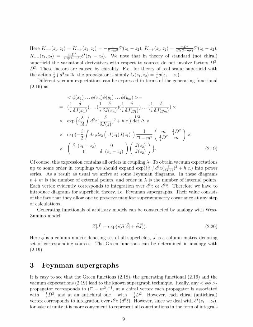
Here K+−(z1, z2) = K−+(z1, z2) = − 12−m2 δ

8(z1 − z2), K++(z1, z2) = mD2

42(2−m2)δ8(z1 − z2),

K−−(z1, z2) = mD2

42(2−m2)δ8(z1 − z2). We note that in theory of standard (not chiral)

superfield the variational derivatives with respect to sources do not involve factors D2,D2. These factors are caused by chirality. F.e. for theory of real scalar superfield withthe action 1

2

∫

d8zv2v the propagator is simply G(z1, z2) = 12δ(z1 − z2).

Different vacuum expectations can be expressed in terms of the generating functional(2.16) as

< φ(x1) . . . φ(xn)φ(y1) . . . φ(ym) >=

= (1

i

δ

δJ(x1)) . . . (

1

i

δ

δJ(xn))(

1

i

δ

δJ(y1)) . . . (

1

i

δ

δJ(ym)) ×

× exp

iλ

3!

∫

d6z(δ

δJ(z))3 + h.c.)

−1/2

det ∆ ×

× exp(− i

2

∫

dz1dz2(

J(z1)J(z1)) 1

2 −m2

(

m 14D2

14D2 m

)

×

×(

δ+(z1 − z2) 00 δ−(z1 − z2)

)(

J(z2)J(z2)

)

. (2.19)

Of course, this expression contains all orders in coupling λ. To obtain vacuum expectationsup to some order in couplings we should expand exp(i λ

3!

∫

d6z( δδJ(z)

)3 + h.c.) into powerseries. As a result as usual we arrive at some Feynman diagrams. In these diagramsn +m is the number of external points, and order in λ is the number of internal points.Each vertex evidently corresponds to integration over d6z or d6z. Therefore we have tointroduce diagrams for superfield theory, i.e. Feynman supergraphs. Their value consistsof the fact that they allow one to preserve manifest supersymmetry covariance at any stepof calculations.

Generating functionals of arbitrary models can be constructed by analogy with Wess-Zumino model:

Z[ ~J ] = exp(i(S[~φ] + ~φ ~J)). (2.20)

Here ~φ is a column matrix denoting set of all superfields, ~J is a column matrix denotingset of corresponding sources. The Green functions can be determined in analogy with(2.19).

3 Feynman supergraphs

It is easy to see that the Green functions (2.18), the generating functional (2.16) and thevacuum expectations (2.19) lead to the known supergraph technique. Really, any < φφ >-propagator corresponds to (2 −m2)−1, at a chiral vertex each propagator is associatedwith −1

4D2, and at an antichiral one – with −1

4D2. However, each chiral (antichiral)

vertex corresponds to integration over d6z (d6z). However, since we deal with δ8(z1 − z2),for sake of unity it is more convenient to represent all contributions in the form of integrals

9

over d8z via the rule d6z(−14)D2F =

∫

d8zF . As a result,∫

d6zΦn-vertex is associatedwith n− 1 (−1

4D2) factors, and

∫

d6zΦm-vertex – with m− 1 (−14D2)-factors – of course,

in the case when all superfields are contracted into propagators. And the vertex d8zΦmΦn

in the same case – with m factors and n (−14D2) factors. Here and further we refer to

superfields contracted into propagators as to the quantum ones. We see that the numberof D2, D2 factors for such vertices is number of antichiral (chiral) quantum superfieldsassociated with this vertex. There is no D, D-factors arisen from propagators of non-chiral (f.e. real) superfields. The propagator < φφ > (< φφ >) corresponds to mD2

42(2−m2)

( mD2

42(2−m2)). However, only quantum fields (i.e. those ones contracted into propagators)

correspond to D2, D2 factors. External lines do not carry such a factor, and if one, two...n chiral (antichiral) superfields associated with the vertex are external the number of D2

(D2) factors corresponding to this vertex is less by one, two... n than in the case whenall superfields are contracted to propagators.

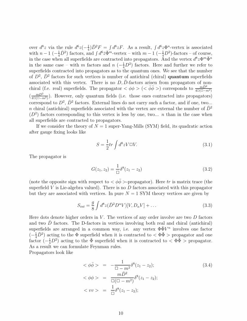
If we consider the theory of N = 1 super-Yang-Mills (SYM) field, its quadratic actionafter gauge fixing looks like

S =1

2tr∫

d8zV2V. (3.1)

The propagator is

G(z1, z2) =1

2δ8(z1 − z2) (3.2)

(note the opposite sign with respect to < φφ >-propagator). Here tr is matrix trace (thesuperfield V is Lie-algebra valued). There is no D factors associated with this propagatorbut they are associated with vertices. In pure N = 1 SYM theory vertices are given by

Sint =g

8

∫

d8z(D2DαV )[V,DαV ] + . . . (3.3)

Here dots denote higher orders in V . The vertices of any order involve are two D factorsand two D factors. The D-factors in vertices involving both real and chiral (antichiral)superfields are arranged in a common way, i.e. any vertex ΦΦV n involves one factor(−1

4D2) acting to the Φ superfield when it is contracted to < ΦΦ > propagator and one

factor (−14D2) acting to the Φ superfield when it is contracted to < ΦΦ > propagator.

As a result we can formulate Feynman rules.Propagators look like

< φφ > = − 1

2 −m2δ8(z1 − z2); (3.4)

< φφ > =mD2

2(2 −m2)δ8(z1 − z2);

< vv > =1

2δ8(z1 − z2);

10

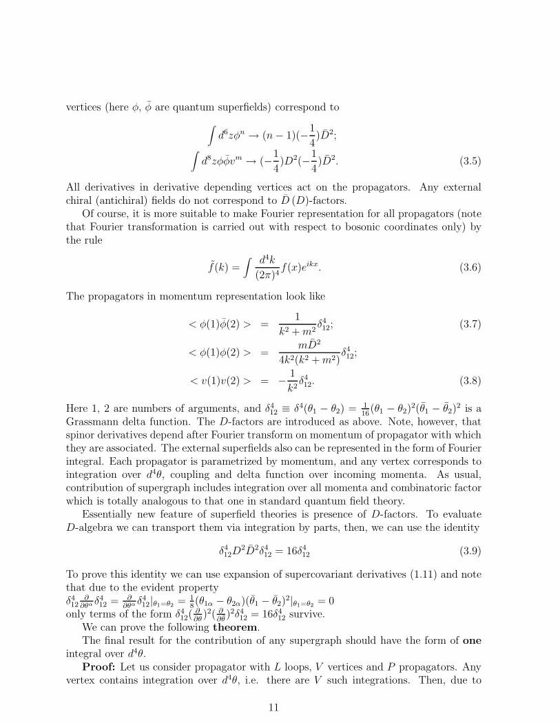
vertices (here φ, φ are quantum superfields) correspond to

∫

d6zφn → (n− 1)(−1

4)D2;

∫

d8zφφvm → (−1

4)D2(−1

4)D2. (3.5)

All derivatives in derivative depending vertices act on the propagators. Any externalchiral (antichiral) fields do not correspond to D (D)-factors.

Of course, it is more suitable to make Fourier representation for all propagators (notethat Fourier transformation is carried out with respect to bosonic coordinates only) bythe rule

f(k) =∫

d4k

(2π)4f(x)eikx. (3.6)

The propagators in momentum representation look like

< φ(1)φ(2) > =1

k2 +m2δ412; (3.7)

< φ(1)φ(2) > =mD2

4k2(k2 +m2)δ412;

< v(1)v(2) > = − 1

k2δ412. (3.8)

Here 1, 2 are numbers of arguments, and δ412 ≡ δ4(θ1 − θ2) = 1

16(θ1 − θ2)

2(θ1 − θ2)2 is a

Grassmann delta function. The D-factors are introduced as above. Note, however, thatspinor derivatives depend after Fourier transform on momentum of propagator with whichthey are associated. The external superfields also can be represented in the form of Fourierintegral. Each propagator is parametrized by momentum, and any vertex corresponds tointegration over d4θ, coupling and delta function over incoming momenta. As usual,contribution of supergraph includes integration over all momenta and combinatoric factorwhich is totally analogous to that one in standard quantum field theory.

Essentially new feature of superfield theories is presence of D-factors. To evaluateD-algebra we can transport them via integration by parts, then, we can use the identity

δ412D

2D2δ412 = 16δ4

12 (3.9)

To prove this identity we can use expansion of supercovariant derivatives (1.11) and notethat due to the evident propertyδ412

∂∂θα δ

412 = ∂

∂θα δ412|θ1=θ2 = 1

8(θ1α − θ2α)(θ1 − θ2)

2|θ1=θ2 = 0only terms of the form δ4

12(∂∂θ

)2( ∂∂θ

)2δ412 = 16δ4

12 survive.We can prove the following theorem.The final result for the contribution of any supergraph should have the form of one

integral over d4θ.Proof: Let us consider propagator with L loops, V vertices and P propagators. Any

vertex contains integration over d4θ, i.e. there are V such integrations. Then, due to

11

(3.7) any propagator carries a delta function over Grassmann coordinates, i.e. there areP delta functions. Then, in any loop we can reduce the number of delta functions byone using identity (3.9), i.e. there are P −L independent delta functions. As a result wecan carry out P − L integrations from V , and after D-algebra transformations we staywith V − (P − L) integrations. And V − (P − L) = 1, therefore the result contains oneintegration over d4θ. The theorem is proved [15].

This theorem is often called non-renormalization theorem. It means that all quantumcorrections are local in θ-space. This theorem is often naively treated as a proof of absenceof chiral corrections (proportional to integral over d2θ). However, such interpretation iswrong since any contribution in the form of integral over chiral subspace can be rewrittenas an integral over whole superspace using identity

∫

d6zf(Φ) =∫

d8z(−D2

42)f(Φ) (3.10)

(this observation was firstly made in [16], its consequences will be studied further).Now let us study evaluation of contributions from supergraphs. The algorithm of it is

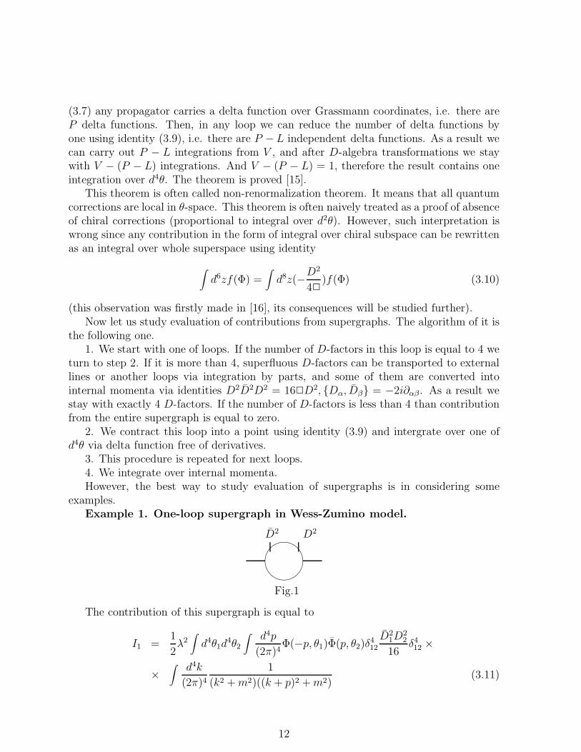
the following one.1. We start with one of loops. If the number of D-factors in this loop is equal to 4 we

turn to step 2. If it is more than 4, superfluous D-factors can be transported to externallines or another loops via integration by parts, and some of them are converted intointernal momenta via identities D2D2D2 = 162D2, Dα, Dβ = −2i∂αβ . As a result westay with exactly 4 D-factors. If the number of D-factors is less than 4 than contributionfrom the entire supergraph is equal to zero.

2. We contract this loop into a point using identity (3.9) and intergrate over one ofd4θ via delta function free of derivatives.

3. This procedure is repeated for next loops.4. We integrate over internal momenta.However, the best way to study evaluation of supergraphs is in considering some

examples.Example 1. One-loop supergraph in Wess-Zumino model.

&%'$D2D2

Fig.1

The contribution of this supergraph is equal to

I1 =1

2λ2∫

d4θ1d4θ2

∫

d4p

(2π)4Φ(−p, θ1)Φ(p, θ2)δ

412

D21D

22

16δ412 ×

×∫

d4k

(2π)4

1

(k2 +m2)((k + p)2 +m2)(3.11)

12

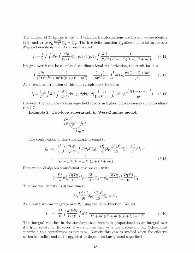
The number of D-factors is just 4. D-algebra transformations are trivial: we use identity

(3.9) and write δ412D2

1D22

16δ412 = δ4

12. The free delta function δ412 allows us to integrate over

d4θ2 and denote θ1 = θ. As a result we get

I1 =1

2λ2∫

d4θ∫

d4p

(2π)4Φ(−p, θ)Φ(p, θ)

∫

d4k

(2π)4

1

(k2 +m2)((k + p)2 +m2)(3.12)

Integral over k can be calculated via dimensional regularization, the result for it is

∫

d4k

(2π)4

1

(k2 +m2)((k + p)2 +m2)=

1

16π2(1

ǫ−∫ 1

0dt log

p2t(1 − t) +m2

µ2) (3.13)

As a result, contribution of this supergraph takes the form

I1 =1

2λ2∫

d4θ∫

d4p

(2π)4Φ(−p, θ)Φ(p, θ)

1

16π2(1

ǫ−∫ 1

0dt log

p2t(1 − t) +m2

µ2) (3.14)

However, the regularization in superfield theory in higher loops possesses some peculiari-ties [17].

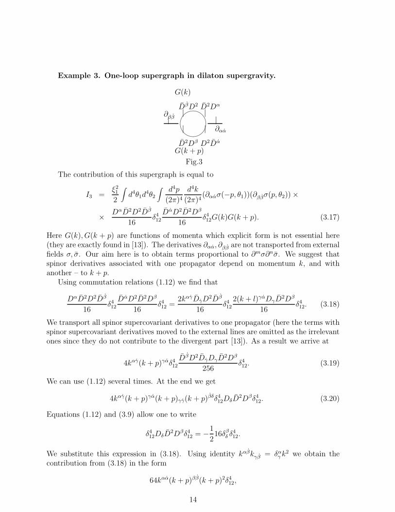
Example 2. Two-loop supergraph in Wess-Zumino model.

&%'$

D2

D2 D2-- -

Fig.2

|D2

The contribution of this supergraph is equal to

I2 =λ2

6

∫

d4kd4l

(2π)8

∫

d4θ1d4θ2(−

D21

4)δ4

12

D21D

22

16δ412(−

D22

4)δ4

12 ×

× 1

(k2 +m2)(l2 +m2)((k + l)2 +m2)(3.15)

First we do D-algebra transformations: we can write

(−D21

4)δ4

12

D21D

22

16δ412(−

D22

4)δ4

12 = δ412

D21D

22

16δ412

D21D

22

16δ412

Then we use identity (3.9) two times:

δ412

D21D

22

16δ412

D21D

22

16δ412 = δ4

12

As a result we can integrate over θ2 using the delta function. We get

I2 =λ2

6

∫ d4kd4l

(2π)8

∫

d4θ11

(k2 +m2)(l2 +m2)((k + l)2 +m2)(3.16)

This integral vanishes in the standard case since it is proportional to an integral overd4θ from constant. However, if we suppose that m is not a constant but θ-dependentsuperfield this contribution is not zero. Namely this case is studied when the effectiveaction is studied and m is suggested to depend on background superfields.

13

Example 3. One-loop supergraph in dilaton supergravity.

&%'$

| |∂αα

∂ββ

|

|

|

|DβD2

D2Dβ D2Dα

D2Dα

G(k)

G(k + p)

Fig.3

The contribution of this supergraph is equal to

I3 =ξ21

2

∫

d4θ1d4θ2

∫

d4p

(2π)4

d4k

(2π)4(∂αασ(−p, θ1))(∂ββσ(p, θ2)) ×

× DαD2D2Dβ

16δ412

DαD2D2Dβ

16δ412G(k)G(k + p). (3.17)

Here G(k), G(k + p) are functions of momenta which explicit form is not essential here(they are exactly found in [13]). The derivatives ∂αα, ∂ββ are not transported from externalfields σ, σ. Our aim here is to obtain terms proportional to ∂mσ∂nσ. We suggest thatspinor derivatives associated with one propagator depend on momentum k, and withanother – to k + p.

Using commutation relations (1.12) we find that

DαD2D2Dβ

16δ412

DαD2D2Dβ

16δ412 =

2kαγDγD2Dβ

16δ412

2(k + l)γαDγD2Dβ

16δ412. (3.18)

We transport all spinor supercovariant derivatives to one propagator (here the terms withspinor supercovariant derivatives moved to the external lines are omitted as the irrelevantones since they do not contribute to the divergent part [13]). As a result we arrive at

4kαγ(k + p)γαδ412

DβD2DγDγD2Dβ

256δ412. (3.19)

We can use (1.12) several times. At the end we get

4kαγ(k + p)γα(k + p)γγ(k + p)βδδ412DδD

2Dβδ412. (3.20)

Equations (1.12) and (3.9) allow one to write

δ412DδD

2Dβδ412 = −1

216δβδ δ

412.

We substitute this expression in (3.18). Using identity kαβkγβ = δαγ k2 we obtain the

contribution from (3.18) in the form

64kαα(k + p)ββ(k + p)2δ412,

14

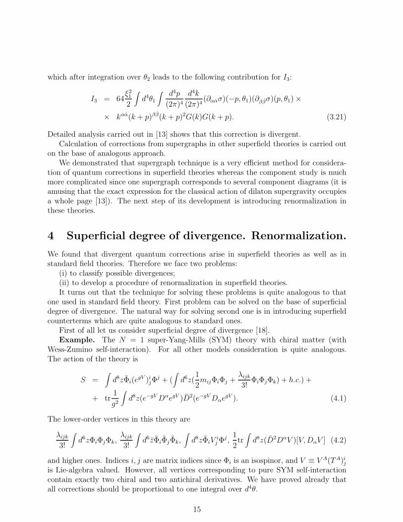
which after integration over θ2 leads to the following contribution for I3:

I3 = 64ξ21

2

∫

d4θ1

∫

d4p

(2π)4

d4k

(2π)4(∂αασ)(−p, θ1)(∂ββσ)(p, θ1) ×

× kαα(k + p)ββ(k + p)2G(k)G(k + p). (3.21)

Detailed analysis carried out in [13] shows that this correction is divergent.Calculation of corrections from supergraphs in other superfield theories is carried out

on the base of analogous approach.We demonstrated that supergraph technique is a very efficient method for considera-

tion of quantum corrections in superfield theories whereas the component study is muchmore complicated since one supergraph corresponds to several component diagrams (it isamusing that the exact expression for the classical action of dilaton supergravity occupiesa whole page [13]). The next step of its development is introducing renormalization inthese theories.

4 Superficial degree of divergence. Renormalization.

We found that divergent quantum corrections arise in superfield theories as well as instandard field theories. Therefore we face two problems:

(i) to classify possible divergences;(ii) to develop a procedure of renormalization in superfield theories.It turns out that the technique for solving these problems is quite analogous to that

one used in standard field theory. First problem can be solved on the base of superficialdegree of divergence. The natural way for solving second one is in introducing superfieldcounterterms which are quite analogous to standard ones.

First of all let us consider superficial degree of divergence [18].Example. The N = 1 super-Yang-Mills (SYM) theory with chiral matter (with

Wess-Zumino self-interaction). For all other models consideration is quite analogous.The action of the theory is

S =∫

d8zΦi(egV )ijΦ

j + (∫

d6z(1

2mijΦiΦj +

λijk3!

ΦiΦjΦk) + h.c.) +

+ tr1

g2

∫

d8z(e−gVDαegV )D2(e−gVDαegV ). (4.1)

The lower-order vertices in this theory are

λijk3!

∫

d6zΦiΦjΦk,λijk3!

∫

d6zΦiΦjΦk,∫

d8zΦiVij Φ

j ,1

2tr∫

d8z(D2DαV )[V,DαV ] (4.2)

and higher ones. Indices i, j are matrix indices since Φi is an isospinor, and V ≡ V A(TA)ijis Lie-algebra valued. However, all vertices corresponding to pure SYM self-interactioncontain exactly two chiral and two antichiral derivatives. We have proved already thatall corrections should be proportional to one integral over d4θ.

15

As usual, the superficial degree of divergence (SDD) is the order of the integral overinternal momenta for corresponding contribution, or, as is the same, as a degree of homo-geneity of diagram in momenta, considered after evaluation of D-algebra transformations[10]. The only difference of the SDD in our case is the additional impact from D-factors.

It is easy to see that contributions to the SDD are generated by momentum dependingfactors in propagators and vertices (as usual, any internal momentum k gives contribu-tion 1), loop integrations, or, in other words, by manifest momentum dependence whichis associated with propagators and loop integration, and by D-factors which are asso-ciated with propagators and vertices (note that due to identities D2D2D2 = 162D2,Dα, Dα = −2i∂αα one chiral derivative combined with an antichiral one can be con-verted to one momentum; therefore any D-factor contribute to the SDD with 1/2). Ifnot all spinor derivatives are converted to internal momenta, the SDD from supergraphevidently decreases.

Let us consider arbitrary supergraph with L loops, V vertices, P propagators (C ofthem are < φφ >, < φφ > -propagators) and E external lines (Ec of them are chiral).We denote the SDD as ω.

Any integration over internal momentum (i.e. over d4k) contributes to SDD with 4.Since the number of integrations over internal momenta is the number of loops, the totalcontribution from all such integrations is 4L. Any propagator includes 1

k2+m2 or 1k2 (3.7),

hence contribution of all propagators is equal to −2P . Since < ΦΦ >,< ΦΦ >-propagatorcontains additional 1

k2 these propagators give additional contribution −2C. Thereforemanifest dependence of momenta gives contribution to ω equal to 4L− 2P − 2C.

Now let us consider contribution of D-factors to SDD. Each vertex (both pure gaugeone and that one containing chiral superfields) without external chiral (antichiral) linescontains fourD-factors (4.2) since any superfield φ (contracted to propagator) correspondsto D2, and φ – to D2. Therefore each vertex gives contribution 2. However, external chiral(antichiral) lines do not correspond to D-factors. As a result, any external line decreasesω by 1, Each < φφ >,< φφ >-propagator contains a factor D2 (D2) with contribution 1.Then, due to identity (3.9) contraction of any loop into a point decreases the number ofD-factors which can be converted to internal momenta by 4, and ω – by 2. As a resultthe total contribution of D-factors to ω is equal to 2V −Ec − 2L+ C (remind that eachD-factor contributes to ω with 1/2).

Therefore SDD is equal to

ω = 4L− 2P − 2C + 2V − Ec − 2L+ C = 2L− 2P + 2V − C − Ec. (4.3)

Using known topological identity L+ V − P = 1 we have

ω = 2 − C − Ec. (4.4)

Really, the SDD can be lower than (4.4) if some of D-factors are transported to externallines and do not generate internal momenta. If ND D-factors are moved to external linesthe ω is equal to

ω = 2 − C − Ec −1

2ND. (4.5)

16

This is the final expression for the SDD. As usual, at ω ≥ 0 supergraph diverges, and atω < 0 – converges. We note that:1. ω ≤ 2 hence SDD is restricted from above.2. As the number of external lines grows, ω decreases. Therefore the number of divergentstructures is essentially restricted – it is finite (really, there can be no more than two exter-nal chiral legs and no more than two < ΦΦ >,< ΦΦ > propagators). And if the numberof divergent structures is finite the theory is renormalizable. Hence we shown that thetheory including chiral superfields with Wess-Zumino-type interaction and gauge super-fields with action (4.1) is renormalizable. This is quite natural since the mass dimensionof all couplings in this theory is zero.

However, non-renormalizable superfield theories also exist.Example. General chiral superfield model [12].The action of the model is

S =∫

d8zK(Φ, Φ) + (∫

d6zW (Φ) + h.c.) =

=∫

d8zΦΦ + [∫

d6z(1

2mΦ2 +

λ

3!Φ3) + h.c.] + (4.6)

+∫

d8z[K12ΦΦ2 +K21ΦΦ2 +∞∑

m,n=2

1

m!n!KmnΦ

nΦm] + (∫

d6z∞∑

l=4

Wn

n!Φn + h.c.).

Here Kij ,Wl are constants.Propagators in the theory are just (3.7), their contribution to SDD is equal to 4L−2P−

2C as above. However, the contribution from D-factors differs. Any vertex KnmΦnΦm

corresponds to n D2-factors and m D2-factors. The total contribution to ω from all suchvertices is

∑

Vt(nv +mv), i.e. sum of n and m over all vertices corresponding to integral

over total superspace. Any vertex WlΦl contains an integral over d6z and effectively

corresponds to (l−1) D2-factors. Total contribution from such vertices is∑

Vc(lc−1) (i.e.

sum over all purely chiral or antichiral vertices). Again external lines decrease the numberof D2 (D2)-factors by 2Ec (Ec is a number of external lines), each < ΦΦ >,< ΦΦ >-propagators carries one D2 (D2)-factor. Contraction of each loop to a point decreases thenumber of D-factors by 4. Hence the total number of D-factors is

2∑

Vt

(nv +mv) + 2∑

Vc

(lc − 1) − 2Ec − 4L+ 2C. (4.7)

Contribution to SDD from D-factors is their number divided by two. Therefore totalSDD is equal to

ω = 4L− 2P − 2C +1

2(2∑

Vt

(nv +mv) + 2∑

Vc

(lc − 1) − 2Ec − 4L+ 2C) =

= 2 − 2V − C − 2Ec + [∑

Vt

(nv +mv) +∑

Vc

(lc − 1)]. (4.8)

Here we used 2L − 2P = 2 − 2V . However, any vertex gives contribution −2 to term−2V and lc − 1 or nv + mv to other terms of ω. It is evidently that either lc − 1 or

17

nv + mv can be more than 2 since either lc ≥ 3 or nv + mv ≥ 3. Hence in general case∑

Vt(nv +mv)+

∑

Vc(lc−1)−2V ≥ 0, the number of divergent structures is not restricted,

and the theory is non-renormalizable. This is quite natural since constants Kij (if i or jno less than 2) and Wl (if l ≥ 4) have negative mass dimension.

The next problem is introduction of regularization. The most natural way of intro-ducing regualarization in supersymmetric theories is dimensional regularization. It canbe introduced as usual: integral

∫ d4k

(2π)4

1

(k2 +m2)N

is replaced by∫

d4+ǫk

(2π)4+ǫ

1

(k2 +m2)N.

All divergences corresponds to poles in ǫ (no more than 1ǫL

for L-loop correction).However, there are some peculiarities. First of all, at component level any supersym-

metric action includes spinors and hence γ-matrices which are well defined if and only ifthe dimension of space-time is integer. Therefore we must use some modification of thedimensional regularization called dimensional reduction. According to it all objects withwell behaviour only at separate dimensions (such as spinors and γ-matrices) are evaluatedat these dimensions (or namely at dimension equal to 4), and integrals over momenta – atarbitrary dimension. However, dimensional reduction leads to some difficulties in calcula-tion of higher loop corrections since many supergraphs involve contractions of essentiallyfour-dimensional objects, such as Levi-Civita tensor ǫabcd, with d-dimensional objects, andsuch contractions need additional definition. As a result frequently the ambiguities arise.However, such phenomena are observed only beyond two loops.

We also can use analytic regularization which corresponds to change

∫

d4k

(2π)4

1

(k2 +m2)n→∫

d4k

(2π)4

1

(k2 +m2)n+ǫ.

However, this regularization also leads to some difficulties (see discussion of questionsconnected to regularization in supersymmetric theories in [17]).

Technique for renormalization in superfield theories is quite analogous to that one incommon QFT. It is carried out via introduction of counterterms.

Example. Consider one-loop contribution to the kinetic term in Wess-Zumino model.Corresponding supergraph is given by Fig. 1 (see above), its contribution is equal to

I1 =1

2λ2∫

d4θ∫

d4p

(2π)4Φ(−p, θ)Φ(p, θ)

1

16π2(1

ǫ−∫ 1

0dt log

p2t(1 − t) +m2

µ2). (4.9)

We see that this divergence has the form of pole part proportional to 1ǫ. To cancel it we

must add to the initial kinetic term

S =∫

d8zΦ(x, θ)Φ(x, θ) (4.10)

18

(which is just∫ d4p

(2π)4d4θΦ(−p, θ)Φ(p, θ)) a counterterm

∆Scountr = − λ2

32π2ǫ

∫

d8zΦ(z)Φ(z) (4.11)

which corresponds to the replacement of∫

d8zΦΦ in the classical action by∫

d8zZΦ(z)Φ(z)where

Z = 1 − λ2

32π2ǫ(4.12)

is a wave function renormalization.The essential peculiarity of superfield theories is the fact that number of counterterms

in these theories is less than in their non-supersymmetric analogs. For example, Wess-Zumino model is a supersymmetric generalization of φ4-theory, but it possesses onlyrenormalization of kinetic term and no renormalization of couplings. The conclusionabout absence of divergent correction to coupling the λ (or as is the same – to chiralpotential) is also called non-renormalization theorem. However, this theorem does notforbid finite corrections to superpotential which present in massless Wess-Zumino model[19, 20, 21, 22].

Theare are also some interesting properties of renormalization in superfield theories.First, all tadpole-type contributions in Wess-Zumino model vanish: supergraph

&%'$-D2

has contribution proportional to D2δ11 = δ12D2δ12 = 0. The similar situation can occur

in other superfield models involving the Wess-Zumino model as an ingredient. However,in theories including vertices proportional to integral over whole superspace (f.e. dilatonsupergravity) tadpole contributions are not equal to zero [13].

Second, all contributions from vacuum supergraphs are proportional to∫

d4θc (withc is a constant) and also vanish. However, this statement is not true for backgrounddependent propagators. Using of background dependent propagators are very importantmethod for calculation of effective action. Now we turn to its studying.

5 Effective action and loop expansion

Effective action is a central object of quantum field theory. Studying of effective action al-lows to investigate problems of vacuum stability, Green functions, spontaneous symmetrybreaking, anomalies and many other problems.

Effective action in superfield theory is defined as usual as a generating functionalof one-particle-irreducible Green functions. It is obtained as a Legendre transform forgenerating functional of connected Green functions:

Γ[Φ] = W [J ] −∫

dzJ(z)Φ(z). (5.1)

19

Here Γ[Φ] is an effective action, dz denotes integral over the corresponding subspace (d6z

for chiral sources, d8z for general ones), Φ is a set of all superfields, Φ(z) = δW [J ]δJ(x)

is so

called mean field or background field, W [J ] = 1ilogZ[J ] is a generating functional of the

connected Green functions. As usual, Γ[Φ] satisfies the equation

δΓ[Φ]

δΦ(x)= −J(x).

The effective action can be expressed in the form of path integral [23]:

eihΓ[Φ] =

∫

Dφeih(S[φ]+φJ−ΦJ). (5.2)

Here S[φ] is a classical action of the corresponding theory. Note that φ is a variable ofintegration, and Φ is a function of classical source J which does not depend on φ. Weintroduced h by dimensional reasons and to obtain loop expansion. To calculate thisintegral we make change of variables of integration:

φ→ Φ +√hφ.

If we have several fields we can unite them into a column vector, and all consideration isquite analogous. The integral (5.2) after this change takes the form

eihΓ[Φ] =

∫

Dφeih(S[Φ+

√hφ]+

√hφJ). (5.3)

Our aim consists here of the expansion of Γ[φ] in power series in h following the approachdescribed in [23].

First, we expand factor in the exponent into power series in h:

i

hS[Φ +

√hφ] +

i√hφJ =

i

h

(

S[Φ] + S ′[Φ]√hφ+

h

2S

′′

[Φ]φ2 + . . .+

+hn/2

n!S(n)[Φ]φn + . . .

)

. (5.4)

Here S(n)[Φ] denotes n-th variational derivative of the classical action with respect to Φ(integration over corresponding space is assumed). This expansion can be substitutedinto (5.3). We introduce Γ[Φ] = Γ[Φ]− S[Φ] which is a quantum contribution to effectiveaction that can be expanded into power series in h: Γ =

∑∞n=1 h

nΓ(n). As a result we have

eihΓ[Φ] =

∫

Dφ exp[ i

h

(

S[Φ] + S ′[Φ]√hφ+

h

2S

′′

[Φ]φ2 + . . .+hn/2

n!S(n)[Φ]φn + . . .

)]

. (5.5)

Then, the block i√h(S ′[Φ] + J)φ can lead only to one-particle-reducible supergraphs since

its contribution with one quantum field φ can form only one propagator. Hence we canomit this term. Then we can expand the exponent into power series in h:

eihΓ[Φ] =

∫

Dφei2S′′

[Φ]φ2(

1 +i√h

3!S(3)[Φ]φ3 +

ih

4!S(4)[Φ]φ4 +

+ (i√h

3!)2(S(3)[Φ]φ3)2 + . . .

)

. (5.6)

20

At the same time, after substituting the expansion of Γ in the left-hand side of (5.5) into

power series in h we get exp( ihΓ[Φ]) = eiΓ

(1)[Φ](1+ ihΓ(2)[Φ]+ . . .) (here we suppose that his a small parameter). Substituing this expansion into (5.6) and comparing equal powersof h we see that any correction Γ(n) corresponds to some correlator. For example, one-loopcorrection is defined from equation

exp(iΓ(1)[Φ]) =∫

Dφei2S′′

[Φ]φ2

, (5.7)

and two-loop one – from equation

Γ(2) =1

i

∫

Dφe(i2S′′

[Φ]φ2)(

i4!S(4)[Φ]φ4 − 1

(3!)2(S(3)[Φ]φ3)2

)

∫

Dφ exp( i2S ′′[Φ]φ2)

. (5.8)

Here, as usual, integration over coordinates in expressions of the form S(n)[Φ]φn is as-sumed.

We can see that:(i) All odd orders in

√h vanish since they correspond to

∫

Dφφ2n+1 exp( i2S

′′

[Φ]φ2).Due to symmetrical properties this integral is equal to zero.

(ii) All terms beyond first order in h are expressed in the form of some correlators.(iii) One-loop correction (5.7) can be expressed in the form of functional determinant

since∫

Dφ exp(i

2S

′′

[Φ]φ2) = Det−1/2S′′

[Φ], (5.9)

which leads to

Γ(1) =i

2Tr log S

′′

[Φ]. (5.10)

And S′′

[Φ] (further we denote it as ∆) is a some operator. In many cases it has the form∆ = 2 + . . .. We can express one-loop effective action in terms of functional (super)trace

Γ(1) =i

2Tr∫ ∞

0

ds

seis∆. (5.11)

This expression is called Schwinger representation for the one-loop effective action. SignTr denotes both matrix trace tr (if ∆ possesses matrix indices) and functional trace, i.e.

Treis∆ = tr∫

d8z1d8z2δ

8(z1 − z2)eis∆δ8(z1 − z2)

Calculation of eis∆ in field theories is carried out with use of a special procedure calledSchwinger-De Witt method or proper time method [24]. This method will be discussedin the next section.

Let us consider higher loop corrections. From (5.6) it is easy to see that all loopcorrections beyond one-loop order have the form of some correlators, i.e. they include

∫

Dφ exp(i

2S

′′

[Φ]φ2)∏

n

(S(n)[Φ]φn). (5.12)

21

Such correlators can be calculated in the way analogous to standard theory of perturba-tions. We can use expression

∫

Dφφneiφ∆φ = (1

i

δ

δj)n∫

Dφei(φ∆φ+jφ)|j=0, (5.13)

which allows to introduce diagram technique in which the role of vertices is played byS(n)[Φ]φn

n!, and role of propagators – by ∆−1. However since ∆ = S

′′

[Φ] is backgrounddependent (see above) we arrive at background dependent propagators < φ(z1)φ(z2) >=∆−1δ8(z1 − z2). These propagators are known to be found exactly only in some spe-cial cases, the most important of them are: first, constant in space-time backgroundsuperfields, second, the background superfields are only chiral. Further we consider someexamples.

Let us turn again to (5.6). We see that each quantum superfield corresponds toh−1/2, and each vertex – to h−1 (which provides hn/2−1S(n)[Φ]φn). Arbitrary (super)graphwith P propagators and V vertices contain 2P quantum superfields (each propagator isformed by contraction of two superfields). Therefore if this (super)graph contain verticesSn1[Φ]φn1 , Sn2[Φ]φn2 , . . . , SnV [Φ]φnV its power in h is

∑Vi=1(

ni

2−1) = 1

2

∑Vi=1 ni−V . How-

ever,∑Vi=1 ni is just the number of quantum fields associated with all vertices which is

equal to 2P . Therefore the correlator described by this (super)graph has power of h equalto P − V = L − 1, with L is number of loops. But any correlator of the form (5.6) is acontrbution to Γ

h, hence contribution from L-loop (super)graph to Γ is proportional to hL.

Hence we found that the order in h from an arbitrary (super)graph is just the number ofloops in it, and the expansion in powers of h is called loop expansion. As a result we seethat loop corrections can be calculated on the base of special (super)field technique.

Let us make some comments. One of the most frequent questions is: how is thedefinition of (one-loop) correction in effective action in terms of trace of logarithm relatedto expression of the same correction in terms of supergraphs?

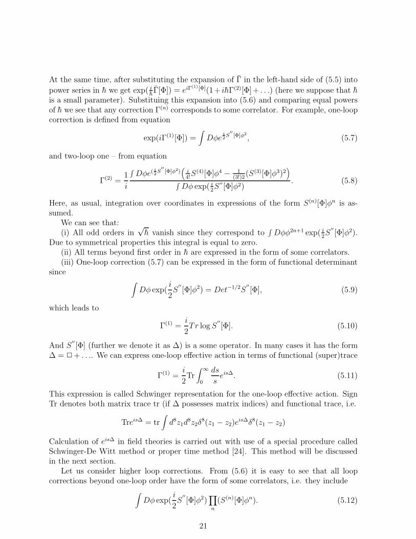
To clarify this relation we give an example. One-loop effective action in Wess-Zuminomodel is given by [25, 10]

Γ(1) =i

2Tr log(2 − 1

4ΨD2 − 1

4ΨD2). (5.14)

Here Ψ is background chiral superfield. This expression can be rewritten as

Γ(1) =i

2Tr log[2(1 − 1

42(ΨD2 + ΨD2))]. (5.15)

Expansion of the logarithm into power series leads to

Γ(1) =i

2Tr

∞∑

n=1

1

n[

1

42(ΨD2 + ΨD2)]n. (5.16)

This expression exactly reproduces the total contribution for the sum of the followingsupergraphs

22

"!#

"!#

Fig.4

"!#

@@

@@ . . .

External lines here are for alternating ΨD2/4 and ΨD2/4, and internal ones are for 2−1.

At the same time, if we consider theory of real scalar superfield u in external chiralsuperfield Ψ with action

S =∫

d8zu(2 − 1

4ΨD2 − 1

4ΨD2)u, (5.17)

it leads just to these supergraphs (if∫

d8zu(−14ΨD2)u and the conjugated term are treated

as vertices), and one-loop effective action for this theory is again given by (5.14).We can see that the expression of one-loop effective action in the form of the trace of

the logarithm of some operator allows to use some special technique which is equivalentto supergraph approach, but more convenient in many cases. This technique is calledproper-time technique.

6 Superfield proper-time technique

As we have already proved, if the quadratic action of a quantum (super)field φ on classicalbackground Φ has the form

∫

dxφ∆[Φ]φ (∫

dx here denotes integral over all (super)space),one-loop effective action in this theory is Γ(1) = i

2Tr

∫∞0

dsseis∆. Therefore we face the

problem of calculating the operator eis∆. In most important cases ∆ = 2 + . . . wheredots denote background dependent terms. It is known [24] that the best way to findthis operator in the case of common field theory is as follows. We introduce U(x, x′|s) =eis∆δ4(x− x′) called Schwinger kernel. Of course, U depends on background superfields.It satisfies the equation:

i∂U

∂s= −U∆. (6.1)

The ∆ is supposed to have form of power series in derivatives. And U satisfies initialcondition

U(x, x′)|s=0 = δ4(x− x′).

In general case U is represented in the form of infinite power series in parameter s (calledproper time) as [24]

U = − i

(4πs)2exp(

i

4s(x− x′)2)

∞∑

n=0

an(is)n. (6.2)

(Ultraviolet) divergences correspond to lower orders of this expansion (note that ultra-violet case corresponds to s → 0, infrared one – to s → ∞). Coefficients an depend on

23

background superfields and their derivatives. We note that if background superfields areput to zero, we arrive at

U (0)(x, x′; s) = eis2δ4(x− x′) = − i

(4πs)2exp(

i

4s(x− x′)2), (6.3)

which satisfies condition

i∫ ∞

0dsU (0)(x, x′; s) =

1

2δ4(x− x′). (6.4)

The approach in case of superfield theories is quite analogous. However, it possessesan essential advantage. In this case it is more convenient to expand Schwinger kernelU(x, x′; s) not in infinite power series in s but in a finite power series in spinor superv-covariant derivatives (these series are finite due to anticommutation properties of spinorderivatives).

Really, in most cases operator ∆ in superfield theories looks like

∆ = 2 +∑

Anm(Dα)n(Dα)m ≡ 2 + ∆ (6.5)

with ∆ is some background dependent operator (in most cases it contains only evenorders in spinor derivatives, here we consider this case), Anm are background dependentcoefficients. We introduce the structure

U(z, z′; s) = exp(is∆)δ8(z − z′) ≡ exp(is∆) exp(is2)δ8(z − z′) (6.6)

(last identity is valid in the case of contributions which do not depend on space-timederivatives of superfields). We substitute natural initial condition

U(z, z′; s)|s=0 = δ8(z − z′).

And exp(is2)δ8(z − z′) = δ4(θ − θ′)U (0)(x, x′; s) where U (0)(x, x′; s) is given by (6.3).Hence

U(z, z′; s) = exp(is∆)U (0)(x, x′; s)δ4(θ − θ′). (6.7)

Therefore we face the problem of calculating U = exp(is∆). The U satisfies the equation

i∂U

∂s= −U∆. (6.8)

It is easy to see that U |s=0 = 1. We expand U into power series in spinor supercovariantderivatives:

U = 1 +1

16A(s)D2D2 +

1

16A(s)D2D2 +

1

8Bα(s)DαD

2 +1

8BαD

αD2 +

+1

4C(s)D2 +

1

4C(s)D2 (6.9)

24

and substitute (6.9) into equation (6.8). As a result we obtain in right-hand side somepower series in spinor derivatives. Comparing coefficients at analogous derivatives inright-hand side and left-hand side of identity we get

1

16A = U∆|D2D2 ;

1

8Bα = U∆|DαD2 ;

1

4C = U∆|D2 (6.10)

and analogous equations for A, Bα, C. Here dot denotes ∂∂is

, and |D2 etc. denotes coeffi-

cient at D2 etc. in U∆. As a result we have system of first-order differential equations oncoefficients determining structure of operator U . Since U |s=0 = 1 we have natural initialconditions

A|s=0 = A|s=0 = Bα|s=0 = Bα|s=0 = C|s=0 = C|s=0 = 0. (6.11)

The system (6.10) with initial conditions (6.11) can be solved like common system ofdifferential equations (note however, that this solution is mostly found in special cases,such as independence on spinor derivatives of background superfields, or dependence onchiral background superfields only etc.)

Then, U(s) (often called heat kernel) can be used for calculation of Green function as

G(z1, z2) = i∫ ∞

0dsUU (0)(x, x′; s)δ4(θ − θ′) (6.12)

(note that U is a differential operator in superspace) and for calculation of one-loopeffective action as

Γ(1) =i

2

∫ ∞

0

ds

s

∫

d8zd8z′δ8(z − z′)UU (0)(x, x′; s)δ4(θ − θ′). (6.13)

As usual,∫

d8z =∫

d4xd4θ, we also use definition (6.3). Then, it is known that δ4(θ −θ)D2D2δ4(θ − θ) = 16δ4(θ − θ), and all products of less number of spinor derivativesgive zero trace. Hence only coefficients of (6.9) giving non-zero contribution to one-loopeffective action are A and A. And one-loop effective action looks like

Γ(1) =i

2

∫ ∞

0

ds

s

∫

d4xd4θ(A(s) + A(s))U (0)(x, x′; s)|x=x′. (6.14)

As a result we developed technique for calculating background dependent propagatorsand one-loop effective action. Application of this technique will be further consideredon examples of several theories. There is an essential modification of this method forsupergauge theories [26].

25

7 Problem of superfield effective potential

Effective potential in standard quantum field theory is defined as the effective Lagrangianconsidered at constant values of scalar fields, and other fields are put to zero. The effectivepotential is used for studying of spontaneous symmetry breaking and vacuum stability[27].

First, let us shortly describe effective potential in common quantum field theory. Theeffective action has the form

Γ[φ] =∫

d4x(−Veff (φ) − 1

2Z(φ)∂mφ∂

mφ+ . . .), (7.1)

where Z(φ) is a some function of φ, and Veff(φ) is effective potential. For slowly varyingfields, therefore,

Γ[φ] = −∫

d4xVeff(φ),

therefore effective potential is a low-energy leading term. It can be represented in theform of loop expansion

Veff(φ) = V (φ) +∞∑

n=1

hnV (n)(φ). (7.2)

For example, consider the theory with action

S =∫

d4x(1

2φ2φ+ V (φ)). (7.3)

After background-quantum splitting φ→ Φ + χ where Φ is background superfield and χis quantum one, we find the quadratic action of quantum superfields

S2 =∫

d4x[1

2χ(2 + V

′′

(Φ))χ] (7.4)

which leads to one-loop effective action Γ(1)[Φ] of the form

Γ(1)[Φ] =i

2Tr log(2 + V

′′

(Φ)). (7.5)

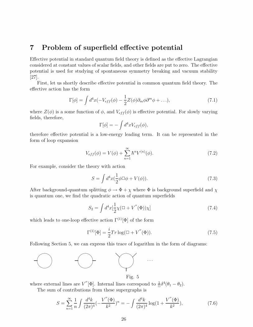
Following Section 5, we can express this trace of logarithm in the form of diagrams:

"!#

"!#

"!#

@@. . .

Fig. 5

where external lines are V′′

[Φ]. Internal lines correspond to 12δ4(θ1 − θ2).

The sum of contributions from these supergraphs is

S =∞∑

n=1

1

n

∫ d4k

(2π)4(−V

′′

(Φ)

k2)n = −

∫ d4k

(2π)4log(1 +

V′′

(Φ)

k2), (7.6)

26

which after integration over d4k and extraction of divergences is equal to [10]

1

64π2(V

′′

(Φ))2(logV

′′

(Φ)

µ2+ C), (7.7)

where C is some constant. The same result can be obtained via proper-time method (seecalculation f.e. in [10]).

Now we turn to superfield case. Let Γ[Φ, Φ] be the renormalized effective action for atheory of chiral and antichiral superfields. We can represent it as

Γ[Φ,Φ] =∫

d8zLeff (Φ, DAΦ, DADBΦ; Φ, DAΦ, DADBΦ) +

+ (∫

d6zL(c)eff (Φ) + h.c.) + . . . (7.8)

Here DAΦ, DADBΦ, . . . are possible supercovariant derivatives of superfields Φ, Φ. Theterm Leff is called general effective Lagrangian, and L(c)

eff is called chiral effective La-grangian. Both these effective Lagrangians can be expanded into power series in superco-variant derivatives of background superfields. Dots denote terms depending on space-timederivatives of Φ, Φ. We note that since chiral effective Lagrangian by definition dependsonly on Φ but not on D2Φ all terms of the form

∫

d6zΦn(D2Φ)m

using relation∫

d6z(− D2

4) =

∫

d8z can be rewritten as

∫

d8zΦnΦ(D2Φ)m−1,

i.e. in the form corresponding to general effective Lagrangian. Therefore here and fur-ther we consider all formally chiral expressions but involving (D2Φ)m as contributions togeneral effective Lagrangian.

We note that all chiral contributions can be also represented as integral over wholesuperspace:

∫

d6zG(Φ) =∫

d8z(−D2

42)G. (7.9)

Further, in component approach we must put scalar component fields to constants, andspinor ones – to zero, f.e. in Wess-Zumino model we write

A = const, F = const, ψα = 0.

However, this condition is not supersymmetric, therefore we use condition of superfieldconstant in space-time:

∂aΦ = 0. (7.10)

27

Since ∂a commutes with all generators of supersymmetry, this condition is supersymmet-ric.

Effective potential is introduced as

Veff =

−∫

d4θLeff − (∫

d2θL(c)eff + h.c.)

|∂aΦ=∂aΦ=0. (7.11)

The minus sign is put by convention. We can introduce general effective potentialLeff |∂aΦ=∂aΦ=0 and chiral effective potential L(c)

eff |∂aΦ=0. It is easy to see that the gen-eral effective potential can be expressed as

Leff = K(Φ, Φ) + F(DαΦ, DαΦ, D2Φ, D2Φ; Φ, Φ) (7.12)

with F|DαΦ,DαΦ,D2Φ,D2Φ=0 = 0. The K is called kahlerian effective potential, and F iscalled auxiliary fields’ effective potential, it is at least of third order in auxiliary fields ofΦ and Φ. These objects can be represented in the form of loop expansion:

K(Φ, Φ) = K0(Φ, Φ) +∞∑

L=1

hLKL(Φ, Φ) (7.13)

F =∞∑

L=1

hLFL (7.14)

(the term corresponding to L = 0 in the expression for F is absent for theories which donot include derivative depending terms in the classical action, such as the Wess-Zuminomodel), and

L(c)eff(Φ) = L(c)(Φ) +

∞∑

L=1

hLL(c)L (Φ). (7.15)

Here KL, FL,L(c)L are quantum corrections. For Wess-Zumino model L(c)

1 = 0, however,in some quantum theories (f.e. in N = 1 super-Yang-Mills theory with chiral matter)one-loop contribution to chiral effective potential exists [20].

The expansion of the effective potential by the rules (7.11–7.15) can be applied for allsuperfield theories including noncommutative ones. However, we note that effective poten-tial in theories including gauge superfields must depend on them in a special way. Really,effective action in such theories should be expressed in terms of some gauge convariantconstructions, f.e. in background field method gauge superfield is either incorporated tochiral superfields or presents in supercovariant derivatives and gauge invariant superfieldstrengths [28, 10].

Let us give a few remarks about the method of calculating effective potential. The bestway for it is, of course, using of background dependent propagators which are expressed interms of common propagators and background superfields. Background dependent propa-gators can be in certain cases exactly found. To calculate kahlerian effective potential andauxiliary fields’ effective potential one can straightforwardly omit all space-time deriva-tives, moreover, to study kahlerian effective potential one can omit ALL supercovariantderivatives and treate background superfields as constants until final integration. Thecalculation of chiral effective potential, however, is characterized by some difficulties. Wewill study an approach to it on example of Wess-Zumino model.

28

8 Wess-Zumino model and problem of chiral effective

potential

Now we turn to consideration of superfield effective potential in Wess-Zumino model.Here we follow the papers [21, 22, 25] and book [10].

The superfield action of Wess-Zumino model is given by (2.9). Following loop expan-sion approach we carry out background-quantum splitting by the rule

Φ → Φ +√hφ;

Φ → Φ +√hφ. (8.1)

The expression (5.6) defining effective action under such changes takes the form (hereΓ =

∑∞L=1 h

LΓL)

eihΓ[Φ,Φ] =

∫

DφDφ exp( i

2

(

φφ)

(

ψ −14D2

−14D2 ψ

)(

φφ

)

+

+i√h

3!(λ

3!φ3 + h.c.)

)

. (8.2)

The quadratic action of quantum superfields looks like

S(2) =1

2

(

φφ)

(

ψ −14D2

−14D2 ψ

)(

φφ

)

. (8.3)

And the matrix superpropagator by definition is an operator inverse to

(

ψ −14D2

−14D2 ψ

)(

δ+ 00 δ−

)

. (8.4)

We can see that this matrix superpropagator can be represented in the form

G(z1, z2) =

(

G++(z1, z2) G+−(z1, z2)G−+(z1, z2) G−−(z1, z2)

)

. (8.5)

where + denotes chirality with respect to corresponding argument, and − correspondingly– antichirality.

It turns out to be that in Wess-Zumino model this matrix looks like

G(z1, z2) =1

16

(

D21D

22G

ψv (z1, z2) D2

1D22G

ψv (z1, z2)

D21D

22G

ψv (z1, z2) D2

1D22G

ψv (z1, z2)

)

. (8.6)

where Gψv (z1, z2) = (2 + 1

4ψD2 + 1

4ψD2)−1δ8(z1 − z2). Really, consider relation

(

ψ −14D2

−14D2 ψ

)

1

16

(

D21D

22G

ψv (z1, z2) D2

1D22G

ψv (z1, z2)

D21D

22G

ψv (z1, z2) D2

1D22G

ψv (z1, z2)

)

= −(

δ+ 00 δ−

)

(8.7)

29

and act on both parts of this relation with the operator

(

0 −14D2

−14D2 0

)

.

We get the following system of equations on components of matrix superpropagator G:

2G++ − 1

4D2

1(ψG−+) = 0;

2G−+ − 1

4D2

1ψG++) =1

16D2

1D22δ

8(z1 − z2);

2G−− − 1

4D2

1(ψG+−) = 0;

2G+− − 1

4D2

1(ψG−−) =1

16D2

1D22δ

8(z1 − z2). (8.8)

Straightforward checking shows that components G++, G+−, G−+, G−− given by (8.6) sat-isfy this equation. Thus, we found matrix superpropagator (8.6) which will be used forcalculation of loop corrections.

Let us consider the one-loop effective action. Formally it has the form

Γ(1) = − i

2Tr logG

where matrix superpropagator G is given by (8.6). However, straightforward calculationof this trace is very complicated since the elements of this matrix are defined in differentsubspaces. The one-loop effective action Γ(1) can be obtained from relation

eiΓ(1)

=∫

DφDφ exp( i

2

(

φφ)

(

ψ −14D2

−14D2 ψ

)(

φφ

)

)

. (8.9)

To take this integral we introduce a trick [25] which is used in many theories describingdynamics of chiral superfields.

We consider theory of real scalar superfield with action

S =1

16

∫

d8zvDαD2Dαv. (8.10)

The action is invariant under gauge transformations δv = Λ − Λ (here Λ is chiral, andΛ is antichiral). According to Faddeev-Popov approach, the effective action W for thistheory can be introduced as

eiW =∫

Dvei16

∫

d8zvDαD2Dαvδ(χ). (8.11)

Here δ(χ) is a functional delta function, and χ is a gauge-fixing function. We choose χ inthe form of column matrix

χ =

(

14D2v − φ

14D2v − φ

)

.

30

Note that since supercovariant derivatives are not real we must impose two conditions,and (8.11) takes the form

eiW =∫

Dvei16

∫

d8zvDαD2Dαvδ(1

4D2v − φ)δ(

1

4D2v − φ)det∆, (8.12)

where

∆ =

(

−14D2 00 −1

4D2

)

is a Faddeev-Popov matrix. We note that W is constant by construction. We multiplyleft-hand sides and right-hand sides of (8.9) and (8.12) respectively, as a result we arriveat

eiΓ(1)+W =

∫

DφDφDv exp( i

2

(

φφ)

(

ψ −14D2

−14D2 ψ

)(

φφ

)

+i

16vDαD2Dαv

)

×

× δ(1

4D2v − φ)δ(

1

4D2v − φ)det∆. (8.13)

Integration over φ, φ with use of delta functions leads to

eiΓ(1)+W =

∫

DφDφ exp( i

2v(2 − 1

4ψD2 − 1

4ψD2)v

)

det∆. (8.14)

However, W and det∆ are constants which can be omitted. We also took into accountthat 1

16D2, D2 + 1

8DαD2Dα = 2 [15], hence the one-loop effective action is equal to

Γ(1) =i

2Tr log(2 − 1

4ψD2 − 1

4ψD2) (8.15)

Here as usual ψ = m+ λΦ, ψ = m+ λΦ. This one-loop effective action can be expressedin form of Schwinger expansion:

Γ(1) =i

2Tr∫ ∞

0

ds

sexp(2 − 1

4ψD2 − 1

4ψD2), (8.16)

or, after manifest writing the trace,

Γ(1) =i

2

∫

d8z1d8z2

∫ ∞

0

ds

sδ8(z1 − z2) exp(is(−1

4ψD2 − 1

4ψD2))eis2δ8(z1 − z2). (8.17)

We consider kernel U(ψ|s) = exp(is(−14ψD2 − 1

4ψD2)) ≡ eis∆. It evidently satisfies the

equation∂U

∂s= iU∆.

It turns out to be that if we calculate kahlerian effective potential and all supercovari-ant derivatives from background superfields ψ, ψ are omitted this equation can be easily

31

solved. We express U in the form (6.9). Then U∆ is equal to

U∆ = −1

4ψD2 − 1

4ψD2 −

− 1

4ψA2D2 − 1

4ψA2D2 +

+1

4Bαψ∂

ααDαD2 − 1

4Bαψ∂

ααDαD2 −

− 1

16ψCD2D2 − 1

16ψCD2D2. (8.18)

Comparing coefficients at analogous derivatives in 1i∂U∂s

and U∆ we get the followingsystem of equations

A = −ψC;

Bα = 2iBαψ∂αα;

C = −ψ − ψA2. (8.19)

System for A, B, C has the analogous form with changing ψ → ψ, A → A etc. Here dotdenotes 1

i∂∂s

≡ ∂∂s

. Since U |s=0 = 1, and all terms in expansion of U (6.9) are evidentlylinearly independent, natural initial conditions are

A = A = Bα = Bα = C = C|s=0 = 0. (8.20)

We find that the system of equations for Bα and Bα is closed (it is separated from wholesystem (8.19)) and homogeneous. Initial conditions above make its only solution to bezero, Bα, Bα = 0. The remaining from (8.19) system for A and C (and analogous onefor A and C) can be easily solved like standard system of common first-order differentialequations. Its solution looks like

C = −√

√

√

√

ψ2

ψ(A1

0 exp(iωs) − A20 exp(−iωs))

A = A10 exp(iωs) + A2

0 exp(−iωs) − 1

2(8.21)

Here ω =√

ψψ2. Imposing initial conditions (8.20) allows to fix coefficients A10, A

20. As

a result we get

C = −√

√

√

√

ψ

ψ2sinh(is

√

ψψ2)

A =1

2[cosh(is

√

ψψ2) − 1] (8.22)

Since A is symmetric with respect to change ψ → ψ we find that A = A. We note thatonly A and A contribute to trace in (8.17). Therefore one-loop kahlerian contribution toeffective action is equal to

K(1) =i

2

∫

d4xd4θ∫ ∞

0

ds

s

1

2[cosh(s

√

ψψ2) − 1]U0(x, x′; s)|x=x′. (8.23)

32

Here U0(x, x′; s) is given by (6.3). This function satisfies the equation (see section 6):

2nU0(x, x

′; s)|x=x′ = (∂

∂s)n

−i16π2s2

.

We expand (8.23) into power series:

1

2[cosh(s

√

ψψ2) − 1] =∞∑

n=0

s2n+2 (ψψ)n+1

(2n+ 2)!2n.

And

K(1) =i

2

∫

d4xd4θ∫ ∞

0

ds

s

∞∑

n=0

s2n+2 (ψψ)n+1

(2n+ 2)!2nU0(x, x

′; s)|x=x′ =

= − i

2

∫

d4xd4θ∫ ∞

0

ds

s

∞∑

n=0

s2n+2 (ψψ)n+1

(2n+ 2)!(∂

∂s)n

−i16π2s2

=

= − 1

32π2

∫

d8z∫ ∞

L2

ds

s2

∞∑

n=0

(−1)n(sψψ)n+1(n+ 1)!

(2n+ 2)!. (8.24)

Here we cut integral at lower limit by introducing L2 for regularization. We make thechange sψψ = t. As a result, the one-loop kahlerian contribution to effective action takesthe form

K(1) = − 1

32π2

∫

d8zψψ∫ ∞

ψψL2dt

∞∑

n=0

(n+ 1)!tn+1(−1)n

(2n + 2)!(8.25)

Then,∑∞n=0

(n+1)!tn+1(−1)n

(2n+2)!= t

∫ 10 due

− t4(1−u2). Hence

K(1) = − 1

32π2

∫

d8zψψ∫ ∞

ψψL2

dt

t

∫ 1

0due−

t4(1−u2). (8.26)

At L2 → 0 this integral tends to

K(1) = − 1

32π2ψψ log(µ2L2) − 1

32π2ψψ(log

ψψ

µ2− ξ). (8.27)

where ξ is some constant which can be absorbed into redefinition of µ. We can add thecounterterm 1

32π2ψψ log(µ2L2) to cancel the divergence. Such a counterterm correspondsto renormalization of kinetic term by the rule

Φ → Z1/2Φ; Z = 1 +λ2

32π2log(µ2L2). (8.28)

And the renormalized kahlerian effective potential is

K(1) = − 1

32π2ψψ(log

ψψ

µ2− ξ). (8.29)

33

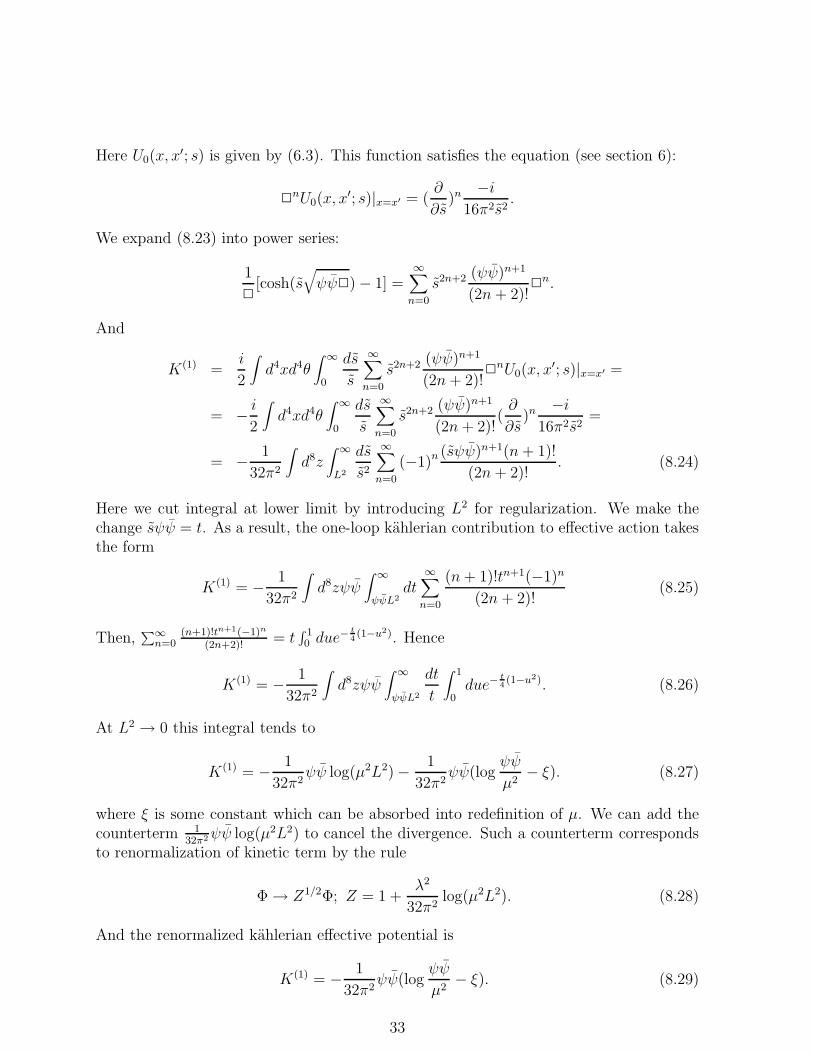
Another way for calculating of kahlerian effective potential consists in summarizing ofcontributions from supergraphs given by Fig. 4. Sum of these contributions looks like[29]

K(1) =∫ d4k

(2π)4

∫

d4θ1 . . . d4θ2n

∞∑

n=1

1

2n(ψψ

k4)D2

4δ12

D2

4δ23 . . .

D2

4δn−1,n

D2

4δn1. (8.30)

which after D-algebra transformations and summation looks like

K(1) =∫

d4−ǫk

(2π)4−ǫ1

2k2log(1 +

ψψ

k2) (8.31)

(here we carried out dimensional regularization by introducing parameter ǫ). Integrationleads to

K(1) =1

32π2[ψψ

ǫ− ψψ log

ψψ

eµ2] (8.32)

where e = exp(1). Subtraction of divergence and redefinition of µ leads to result (8.29).Now we turn to calculation of chiral effective potential. It is not equal to zero for

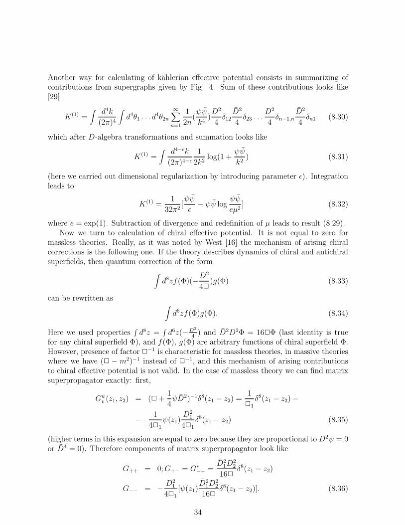
massless theories. Really, as it was noted by West [16] the mechanism of arising chiralcorrections is the following one. If the theory describes dynamics of chiral and antichiralsuperfields, then quantum correction of the form

∫

d8zf(Φ)(−D2

42)g(Φ) (8.33)

can be rewritten as∫

d6zf(Φ)g(Φ). (8.34)

Here we used properties∫

d8z =∫

d6z(−D2

4) and D2D2Φ = 162Φ (last identity is true

for any chiral superfield Φ), and f(Φ), g(Φ) are arbitrary functions of chiral superfield Φ.However, presence of factor 2

−1 is characteristic for massless theories, in massive theorieswhere we have (2 −m2)−1 instead of 2

−1, and this mechanism of arising contributionsto chiral effective potential is not valid. In the case of massless theory we can find matrixsuperpropagator exactly: first,

Gψv (z1, z2) = (2 +

1

4ψD2)−1δ8(z1 − z2) =

1

21δ8(z1 − z2) −

− 1

421

ψ(z1)D2

1

421

δ8(z1 − z2) (8.35)

(higher terms in this expansion are equal to zero because they are proportional to D2ψ = 0or D4 = 0). Therefore components of matrix superpropagator look like

G++ = 0;G+− = G∗−+ =

D21D

22

162δ8(z1 − z2)

G−− = − D21

421[ψ(z1)

D21D

22

162δ8(z1 − z2)]. (8.36)

34

Here ∗ denotes complex conjugation. We note that background chiral superfield ψ is notconstant, otherwise when we arrive at expression proportional to D2ψ we get singularity 0

0

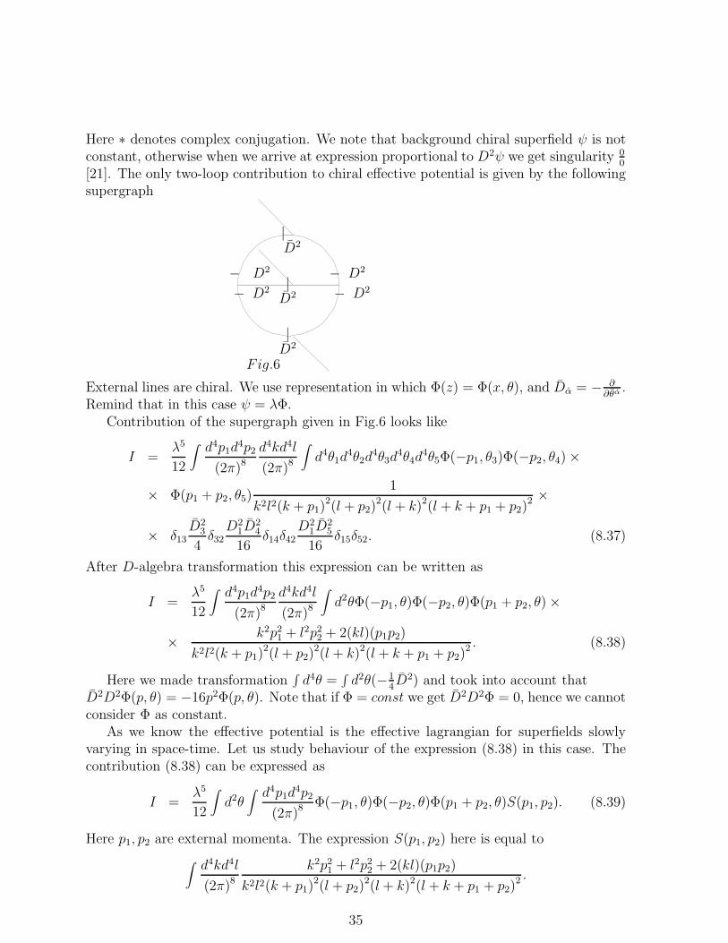
[21]. The only two-loop contribution to chiral effective potential is given by the followingsupergraph

Fig.6

|

D2|

|D2

D2

D2

D2

D2

D2

−−

−−

External lines are chiral. We use representation in which Φ(z) = Φ(x, θ), and Dα = − ∂∂θα .

Remind that in this case ψ = λΦ.Contribution of the supergraph given in Fig.6 looks like

I =λ5

12

∫

d4p1d4p2

(2π)8

d4kd4l

(2π)8

∫

d4θ1d4θ2d

4θ3d4θ4d

4θ5Φ(−p1, θ3)Φ(−p2, θ4) ×

× Φ(p1 + p2, θ5)1

k2l2(k + p1)2(l + p2)

2(l + k)2(l + k + p1 + p2)2 ×

× δ13D2

3

4δ32

D21D

24

16δ14δ42

D21D

25

16δ15δ52. (8.37)

After D-algebra transformation this expression can be written as

I =λ5

12

∫ d4p1d4p2

(2π)8d4kd4l

(2π)8

∫

d2θΦ(−p1, θ)Φ(−p2, θ)Φ(p1 + p2, θ) ×

× k2p21 + l2p2

2 + 2(kl)(p1p2)

k2l2(k + p1)2(l + p2)

2(l + k)2(l + k + p1 + p2)2 . (8.38)

Here we made transformation∫

d4θ =∫

d2θ(−14D2) and took into account that

D2D2Φ(p, θ) = −16p2Φ(p, θ). Note that if Φ = const we get D2D2Φ = 0, hence we cannotconsider Φ as constant.

As we know the effective potential is the effective lagrangian for superfields slowlyvarying in space-time. Let us study behaviour of the expression (8.38) in this case. Thecontribution (8.38) can be expressed as

I =λ5

12

∫

d2θ∫

d4p1d4p2

(2π)8 Φ(−p1, θ)Φ(−p2, θ)Φ(p1 + p2, θ)S(p1, p2). (8.39)

Here p1, p2 are external momenta. The expression S(p1, p2) here is equal to

∫

d4kd4l

(2π)8k2p2

1 + l2p22 + 2(kl)(p1p2)

k2l2(k + p1)2(l + p2)

2(l + k)2(l + k + p1 + p2)2 .

35

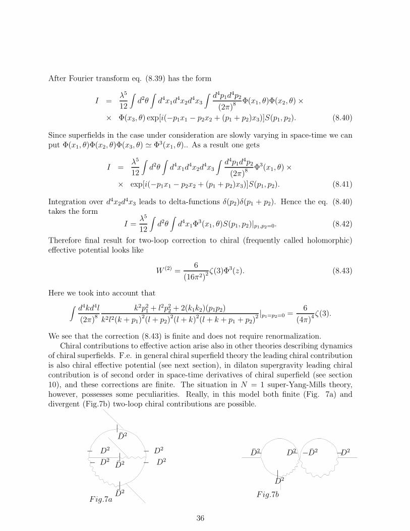
After Fourier transform eq. (8.39) has the form

I =λ5

12

∫

d2θ∫

d4x1d4x2d

4x3

∫

d4p1d4p2

(2π)8 Φ(x1, θ)Φ(x2, θ) ×

× Φ(x3, θ) exp[i(−p1x1 − p2x2 + (p1 + p2)x3)]S(p1, p2). (8.40)

Since superfields in the case under consideration are slowly varying in space-time we canput Φ(x1, θ)Φ(x2, θ)Φ(x3, θ) ≃ Φ3(x1, θ).. As a result one gets

I =λ5

12

∫

d2θ∫

d4x1d4x2d

4x3

∫

d4p1d4p2

(2π)8 Φ3(x1, θ) ×

× exp[i(−p1x1 − p2x2 + (p1 + p2)x3)]S(p1, p2). (8.41)

Integration over d4x2d4x3 leads to delta-functions δ(p2)δ(p1 + p2). Hence the eq. (8.40)

takes the form

I =λ5

12

∫

d2θ∫

d4x1Φ3(x1, θ)S(p1, p2)|p1,p2=0. (8.42)

Therefore final result for two-loop correction to chiral (frequently called holomorphic)effective potential looks like

W (2) =6

(16π2)2 ζ(3)Φ3(z). (8.43)

Here we took into account that

∫

d4kd4l

(2π)8k2p2

1 + l2p22 + 2(k1k2)(p1p2)

k2l2(k + p1)2(l + p2)

2(l + k)2(l + k + p1 + p2)2 |p1=p2=0 =

6

(4π)4 ζ(3).

We see that the correction (8.43) is finite and does not require renormalization.Chiral contributions to effective action arise also in other theories describing dynamics

of chiral superfields. F.e. in general chiral superfield theory the leading chiral contributionis also chiral effective potential (see next section), in dilaton supergravity leading chiralcontribution is of second order in space-time derivatives of chiral superfield (see section10), and these corrections are finite. The situation in N = 1 super-Yang-Mills theory,however, possesses some peculiarities. Really, in this model both finite (Fig. 7a) anddivergent (Fig.7b) two-loop chiral contributions are possible.

Fig.7a

|

D2|

|D2

D2

D2

D2

D2

D2

−−

−−

Fig.7b

−D2 −D2 −D2 −D2

|D2

36

Finite contributions (there are more than 10 supergraphs of the form similar to Fig.

7a [30]) all give contributions to effective potential proportional to ζ(3)(4π)4

Φ3 (cf. (8.43)),i.e. finite chiral contributions are analogous to the case of Wess-Zumino model. As fordivergent contribution given by Fig. 4b it is, after D-algebra transformation, equal to

∫

d2θ∫

d4p1d4p2

(2π)8(p1 + p2)

2∫

d4kd4l

(2π)8

1

k2(k + p1)2(k + p2)2×

× 1

l2(l + p1 + p2)2Φ(−p1, θ)Φ(−p2, θ)Φ(p1 + p2, θ). (8.44)

To obtain the low-energy leading contribution we must consider the limit at p1, p2 → 0.It is known [20] that

limp1,p2→0

(p1 + p2)2∫

d4k

(2π)4

1

k2(k + p1)2(k + p2)2=

1

16π2

∫ 1

0dα

log[α(1 − α)]

1 − α(1 − α)=

C0

16π2,

where C0 is a some constant. The integral over l is divergent, and after dimensionalregularization it is equal to

∫ d4−ǫl

(2π)4−ǫ1

l2(l + p1 + p2)2=

1

16π2(2

ǫ+ log

(p1 + p2)2

µ2).

After cancellation of divergence with help of the appropriate one-loop counterterm andtransforming to coordinate representation we see that expression (8.44) for slowly varyingin space-time superfields takes the form

∫

d6z1

(16π2)2Φ2(z) log(− 2

µ2)Φ(z). (8.45)

Thus, the leading chiral correction in N = 1 super-Yang-Mills theory with chiral matteris nonlocal one (detailed discussion is given in [30]). We note that nonlocal chiral correc-tions in this theory arise also in the pure gauge sector [31]. Hence presence of quantumcontributions to chiral effective Lagrangian is quite characteristic for theories includingchiral superfields.

9 General chiral superfield model

From viewpoint of superstring theory low-energy models of elementary particles are effec-tive theories in which integration over massive string modes is carried out, 10-dimensionalbackground manifold has the formM4×K where M4 is four-dimensional Minkovski space,and K is some six-dimensional compact manifold. Then reduction to M4 is carried out.As a result we arrive at theory in M4 with action [1]

S[Φ, Φ] =∫

d8zK(Φi, Φi) + (∫

d6zW (Φi) + h.c.). (9.1)

We can use matrix denotions via introduction of column vector ~Φ = Φi, after which theconsideration in the case of several chiral superfield is analogous to the case of one chiral

37

superfield (some extensions of this model involving the gauge superfields are given in[32]). We can consider this theory for arbitrary functions K and W . Note that there is nohigher derivatives in the classical action. Therefore the theory with the action (9.1) is themost general theory without higher derivatives describing dynamics of chiral superfield.There are a lot of phenomenological applications of this model in string theory (see [32]and references therein). In general case this theory is nonrenormalizable; however, it isan effective theory aimed for studying of the low-energy domain. Therefore all integralsover momenta are effectively cut by condition p ≪ MString where p is momentum, andMString = 1017GeV ∼ 10−2MP l is a characteristic string mass.

The effective action in the theory, as well as that one in the Wess-Zumino model, canbe presented as a series in supercovariant derivatives DA = (∂a, Dα, Dα) in the form

Γ[Φ,Φ] =∫

d8zLeff (Φ, DAΦ, DADBΦ; Φ, DAΦ, DADBΦ) +

+ (∫

d6zL(c)eff (Φ) + h.c.) + . . . . (9.2)

Here again, like in the Wess-Zumino model, Leff is called general effective lagrangian, L(c)eff

is called chiral effective lagrangian. Both these lagrangians are the series in supercovariantderivatives of superfields and can be written in the form of loop expansion

Leff = Keff(Φ,Φ) + . . . = K(Φ,Φ) +∞∑

n=1

K(n)eff(Φ,Φ);

L(c)eff = Weff(Φ) + . . . = W (Φ) +

∞∑

n=1

W(n)eff (Φ) + . . . . (9.3)

Here dots mean terms depending on covariant derivatives of superfields Φ, Φ. As earlier,the Keff(Φ,Φ) is called kahlerian effective potential, Weff (Φ) is called chiral (or holo-

morphic) effective potential, K(n)eff is a n-th correction to kahlerian potential and W

(n)eff is

a n-th correcton to chiral (holomorphic) potential W .The one-loop contribution to the effective action is totally determined by the quadratic

part of expansion of 1hS[Φ +

√hφ,Φ +

√hφ] in quantum fields φ, φ which looks like

S2 =1

2

∫

d8z(

φ φ)

(

KΦΦ KΦΦ

KΦΦ KΦΦ

)(

φφ

)

+ [∫

d6z1

2W

′′

φ2 + h.c.] (9.4)

and defines the propagators and the the higher terms of expansion define the vertices.

Here KΦΦ = ∂2K(Φ,Φ)∂Φ∂Φ

, KΦΦ = ∂2K(Φ,Φ)∂Φ2 etc, W

′′

= d2WdΦ2 .

The corresponding matrix superpropagator has the form

G(z1, z2) =

(

G++(z1, z2) G+−(z1, z2)G−+(z1, z2) G−−(z1, z2)

)

(9.5)

where + denotes chirality with respect to corresponding argument, and − correspondingly– antichirality. This propagator satisfies the equation

W′′ − 1

4(D2KΦΦ) −1

4~D2KΦΦ

−14~D2KΦΦ W

′′ − 14(D2KΦΦ)

(

G++(z1, z2) G+−(z1, z2)G−+(z1, z2) G−−(z1, z2)

)

=

38

= −(

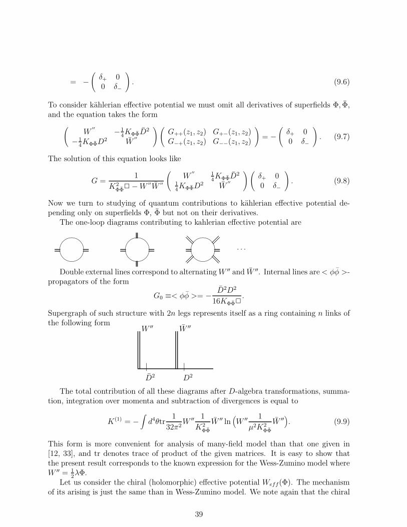
δ+ 00 δ−

)

. (9.6)

To consider kahlerian effective potential we must omit all derivatives of superfields Φ, Φ,and the equation takes the form

(

W′′ −1

4KΦΦD

2

−14KΦΦD

2 W′′

)(

G++(z1, z2) G+−(z1, z2)G−+(z1, z2) G−−(z1, z2)

)

= −(

δ+ 00 δ−

)

. (9.7)

The solution of this equation looks like

G =1

K2ΦΦ2 −W ′′W ′′

(

W′′ 1

4KΦΦD

2

14KΦΦD

2 W′′

)(

δ+ 00 δ−

)

. (9.8)

Now we turn to studying of quantum contributions to kahlerian effective potential de-pending only on superfields Φ, Φ but not on their derivatives.

The one-loop diagrams contributing to kahlerian effective potential are

"!#

"!#

"!#

@@@@

@@@@ . . .

Double external lines correspond to alternatingW ′′ and W ′′. Internal lines are< φφ >-propagators of the form

G0 ≡< φφ >= − D2D2

16KΦΦ2.

Supergraph of such structure with 2n legs represents itself as a ring containing n links ofthe following form

D2

|D2

|

W ′′ W ′′

The total contribution of all these diagrams after D-algebra transformations, summa-tion, integration over momenta and subtraction of divergences is equal to

K(1) = −∫

d4θtr1

32π2W ′′ 1

K2ΦΦ

W ′′ ln(

W ′′ 1

µ2K2ΦΦ

W ′′)

. (9.9)

This form is more convenient for analysis of many-field model than that one given in[12, 33], and tr denotes trace of product of the given matrices. It is easy to show thatthe present result corresponds to the known expression for the Wess-Zumino model whereW ′′ = 1

2λΦ.

Let us consider the chiral (holomorphic) effective potential Weff(Φ). The mechanismof its arising is just the same than in Wess-Zumino model. We note again that the chiral

39

contributions to effective action can be generated by supergraphs containing masslesspropagators only. To find chiral corrections to effective action we put Φ = 0 in eq. (9.4).Therefore here and further all derivatives of K, W and W will be taken at

Φ = 0. Under this condition the action of quantum superfields φ, φ in external superfieldΦ looks like

S[φ, φ,Φ] =1

2

∫

d8z(

φ φ)

(

KΦΦ KΦΦ

KΦΦ KΦΦ

)(

φφ

)

+∫

d6z1

2W

′′

φ2 + . . . . (9.10)

The dots here denote the terms of third, fourth and higher orders in quantum superfields.We call the theory massless if W

′′ |Φ=0 = 0. Further we consider only massless theory.To calculate the corrections to W (Φ) we use supergraph technique (see f.e. [10]). For

this purpose one splits the action (9.10) into sum of free part and vertices of interaction.As a free part we take the action S0 =

∫

d8zφφ. The corresponding superpropagator is

G(z1, z2) = −D21D

22

162δ8(z1 − z2). And the term S[φ, φ,Φ] − S0 will be treated as vertices

where S[φ, φ,Φ] is given by eq. (9.10). Our purpose is to find the first leading contributionto Weff(Φ). As we will show, chiral loop contributions begin with two loops. Thereforewe keep in eq. (9.10) only the terms of second, third and fourth orders in quantum fields.

Non-trivial corrections to chiral potential can arise only if 2L + 1 − nW ′′ − nVc= 0

where L is a number of loops, nW ′′ is a number of vertices proportional to W′′

, nVcis that

one of vertices of third and higher orders in quantum superfields, otherwise correspondingcontribution will either vanish or lead to singularity in the infrared linit. In one-loopapproximation this equation leads to nW ′′ + nVc

= 3. However, all supergraphs satisfyingthis condition have zero contribution. Therefore first correction to chiral effective potentialis two-loop one. In two-loop approximation this equation has the form nW ′′ + nVc

= 5.Since the number of purely chiral (antichiral) vertices independent of W

′′

in two-loopsupergraphs can be equal to 0, 1 or 2, the number of external vertices W

′′

takes valuesfrom 3 to 5.

We note that non-trivial contribution to chiral (holomorphic) effective potential fromany diagram can arise only if the number of D2-factors is more by one than the number ofD2-factors (see details in [34]). The only Green function in the theory is the propagator< φφ >. Therefore total number of quantum chiral superfields φ corresponding to allvertices must be equal to that one of antichiral ones φ. As a result we find that the only

40

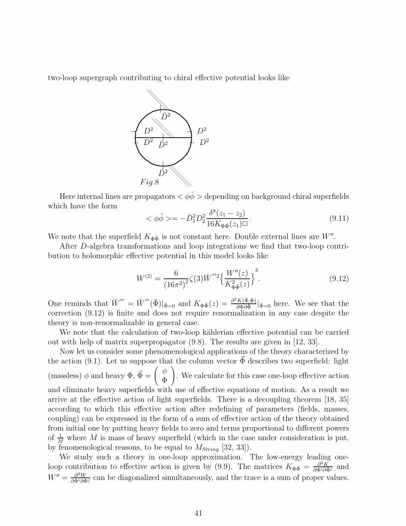
two-loop supergraph contributing to chiral effective potential looks like

Fig.8

|

D2|

|D2

D2

D2

D2

D2

D2

−−

−−

Here internal lines are propagators < φφ > depending on background chiral superfieldswhich have the form

< φφ >= −D21D

22

δ8(z1 − z2)

16KΦΦ(z1)2. (9.11)

We note that the superfield KΦΦ is not constant here. Double external lines are W ′′.After D-algebra transformations and loop integrations we find that two-loop contri-

bution to holomorphic effective potential in this model looks like

W (2) =6

(16π2)2 ζ(3)W′′′2 W ′′(z)

K2ΦΦ(z)

3

. (9.12)

One reminds that W′′′

= W′′′

(Φ)|Φ=0 and KΦΦ(z) = ∂2K(Φ,Φ)∂Φ∂Φ

|Φ=0 here. We see that thecorrection (9.12) is finite and does not require renormalization in any case despite thetheory is non-renormalizable in general case.

We note that the calculation of two-loop kahlerian effective potential can be carriedout with help of matrix superpropagator (9.8). The results are given in [12, 33].

Now let us consider some phenomenological applications of the theory characterized bythe action (9.1). Let us suppose that the column vector ~Φ describes two superfield: light

(massless) φ and heavy Φ, ~Φ =

(

φΦ

)

. We calculate for this case one-loop effective action

and eliminate heavy superfields with use of effective equations of motion. As a result wearrive at the effective action of light superfields. There is a decoupling theorem [18, 35]according to which this effective action after redefining of parameters (fields, masses,coupling) can be expressed in the form of a sum of effective action of the theory obtainedfrom initial one by putting heavy fields to zero and terms proportional to different powersof 1

Mwhere M is mass of heavy superfield (which in the case under consideration is put,

by fenomenological reasons, to be equal to MString [32, 33]).We study such a theory in one-loop approximation. The low-energy leading one-

loop contribution to effective action is given by (9.9). The matrices KΦΦ = ∂2K∂Φi∂Φj and

W ′′ = ∂2W∂Φi∂Φj can be diagonalized simultaneously, and the trace is a sum of proper values.

41

We consider, as an example, the minimal theory [36] with

K = φφ+ ΦΦ; W =M

2Φ2 +

λ

2Φφ2 +

g

3!φ3. (9.13)

After calculations described in [36] and analogous ones to those of Wess-Zumino modelwe get

K(1) = − 1

32π2(R2

1 logR2

1

µ2+R2

2 logR2

2

µ2) (9.14)

where

R1,2 = |λΦ + gφ|2 + 2λ2|φ|2 +M2 ±±

√

(|λΦ + gφ|2 −M2)2 + 4|λ2Φφ+ λMφ + λg|φ|2|2. (9.15)

The low-energy effective action is given by

Γ(1) =∫

d8z(φφ + ΦΦ + hK(1)) + [∫

d6z(M

2Φ2 +

λ

2Φφ2 +

g

3!φ3) + h.c.]. (9.16)

The effective equations of motion for heavy superfield Φ looks like

−1

4D2(Φ + h

∂K(1)

∂Φ) +MΦ +

λ

2φ2 = 0. (9.17)

We can solve this equation by iterative method, i.e. we suppose that

Φ = Φ0 + Φ1 + . . .+ Φn + . . . , (9.18)

with Φk is k-th approximation. Since mass M is very large we suppose that |D2Φ| ≪MΦ.

Zero approximation is obtained from condition MΦ0 + λ2φ2 = 0, i.e. Φ0 = −λφ2

2M. And

k-th approximation is proportional to M−k. Substituting the expansion of Φ (9.18) into(9.17) we get the following recurrent relation for Φn+1:

Φn+1 =D2

4M[Φn + h

∂K(1)

∂Φ|Φ=Φ0+...+Φn

− h∂K(1)

∂Φ|Φ=Φ0+...+Φn−1 ]. (9.19)

As a result, we get the following solution for Φ in leading order

Φ = −λφ2

2M− hD2

64π2M[λgφ(1 + log

2g2|φ|2µ2

)] +O(1

M2). (9.20)

This solution can be substituted into the low-energy effective action (9.16). The effectiveaction of light superfields is defined as

Seff [φ, φ] = Γ(1)[φ, φ; Φ(φ, φ), Φ(φ, φ)] (9.21)

42

where Φ(φ, φ) and the same notation for Φ mean that heavy superfields are expressedin terms of light ones via effective equations of motion. In the case under consideration,effective action of light superfields looks like

Seff = S(0)eff + S

(1)eff +O(

1

M2) (9.22)

where S(0)eff and S

(1)eff are of zeroth and first orders in M−1 respectively. These expressions

look like

S0eff =

∫

d8z[

φφ− h

32π2[4λ2|φ|2(1 + log

2M2

µ2) + 2g2|φ|2 log

2g2|φ|2µ2

] +

+ (∫

d6zg

3!φ3 + h.c.)

]

S(1)eff = − h

32π2M

∫

d8z[

− 2λ2g(φ+ φ)|φ|2 logg2|φ|2M2

+ 2λ2g[φφ2 + h.c.]]

+

+1

M

[

∫

d6z(1

8λ2φ4 − λ2g2(

hD2

64π2(φ(1 + log

2g2|φ|2µ2

))2)

+ h.c.]

. (9.23)

We see that this effective action contains term of the form

− h

32π24λ2|φ|2(1 + log

2M2

µ2)

which increases with growth of M . If we put the renormalization condition log 2M2

µ2 = −1this term vanishes. The effective action, however, in this case takes the form

S0eff =

∫

d8z[

φφ− h

32π22g2|φ|2 log

2g2|φ|2eM2

+

+ (∫

d6zg

3!φ3 + h.c.)

]

. (9.24)

This expression contains the term 2g2|φ|2 log 2g2|φ|2eM2 which also increases as M grows.

Therefore we see that modifications of light superfield effective action caused by presenceof heavy superfields are significant [36].

10 Dilaton supergravity as an example of superfield

theory with higher derivatives

The starting point of our consideration is the supertrace anomaly of matter superfield incurved superspace. The action generating this anomaly is obtained in [37]. In conformallyflat superspace (in which the vector supergravity prepotential Hm is equal to zero) thisaction looks like

ΓA =1

16π2

∫

d8z(8c∂aσ∂aσ +

1

32(32c− b)DασDασ(∂αα(σ + σ) −

− 1

2DασDασ)). (10.1)

43

Here we have used the ”flat” supercovariant derivatives Dα, Dα, ∂αα; and σ = ln Φ,σ = ln Φ.

Let us also consider the superfield action of N=1 supergravity, in conformally flatsuperspace we obtain

SSG = −m2

2

∫

d8zΦΦ + [Λ∫

d6zΦ3 + h.c.], (10.2)

where m2 = 6κ2 , Λ is the cosmological constant and κ is the gravitational constant. We will

investigate the theory action of which is a sum of the actions (10.1) and (10.2) Denoting

Q2

2= 8c, ξ1 =

1

32(4π)2(32c− b), ξ2 = − 1

64(4π)2 (32c− b),

we get a superfield theory in flat superspace with the action of the form

S =∫

d8z(− Q2

2(4π)2 σ2σ + DασDασ ×

× (ξ1∂αα(σ + σ) + ξ2DασDασ) − m2

2eσ+σ) + (Λ

∫

d6ze3σ + h.c.). (10.3)

The Q2, ξ1, ξ2, m2,Λ will be considered as the arbitrary and independent parameters of the

model. We will call the model with action (10.3) the four-dimensional dilaton supergravitymodel.

In order to calculate the counterterms and to find the divergences we should study thestructure of supergraphs of the theory. The strucure of supergraphs is defined by a formof propagators and vertices.

The theory under consideration is characterized by a matrix propagator

G(z, z′) =

(

G++(z, z′) G+−(z, z′)G−+(z, z′) G−−(z, z′)

)

, (10.4)

satisfying the equation

9Λ ( Q2

(4π)22 +m2) D

2

4

( Q2

(4π)22 +m2)D

2

49Λ

(

G++ G+−G−+ G−−

)

=

(

δ+ 00 δ−

)

, (10.5)

where δ+ = −14D2δ8(z1 − z2), δ− = −1

4D2δ8(z1 − z2). The solution of this equation is

written in the form

G =1

81ΛΛ − 2( Q2

16π2 2 +m2)2

[

9Λ −( Q2

16π2 2 +m2) D2

4

−( Q2

16π2 2 +m2)D2

49Λ

]

. (10.6)

This propagator acts on columns

(

φφ

)

, where φ is a chiral superfield and φ is an antichiral

superfield.

44

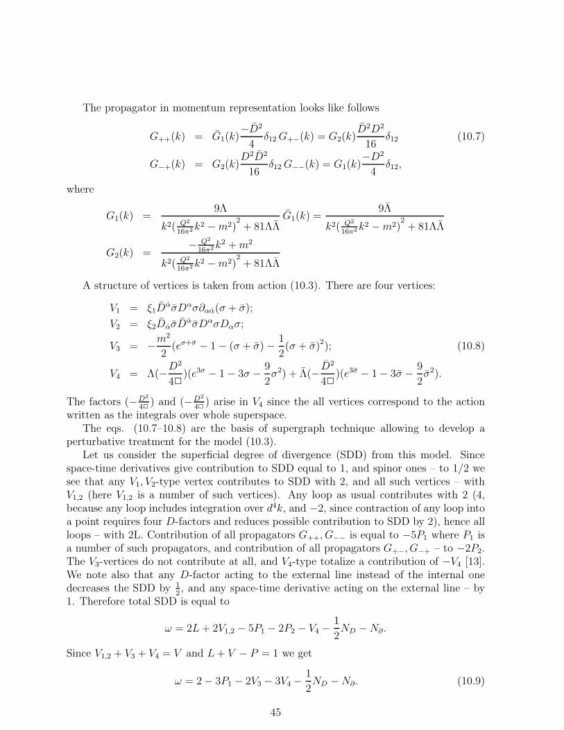
The propagator in momentum representation looks like follows

G++(k) = G1(k)−D2

4δ12G+−(k) = G2(k)

D2D2

16δ12 (10.7)

G−+(k) = G2(k)D2D2

16δ12 G−−(k) = G1(k)

−D2

4δ12,

where

G1(k) =9Λ

k2( Q2

16π2k2 −m2)2+ 81ΛΛ

G1(k) =9Λ

k2( Q2

16π2k2 −m2)2+ 81ΛΛ

G2(k) =− Q2

16π2k2 +m2

k2( Q2

16π2k2 −m2)2+ 81ΛΛ

A structure of vertices is taken from action (10.3). There are four vertices:

V1 = ξ1DασDασ∂αα(σ + σ);

V2 = ξ2DασDασDασDασ;

V3 = −m2

2(eσ+σ − 1 − (σ + σ) − 1

2(σ + σ)2); (10.8)

V4 = Λ(−D2

42)(e3σ − 1 − 3σ − 9

2σ2) + Λ(−D

2

42)(e3σ − 1 − 3σ − 9

2σ2).

The factors (−D2

42) and (−D2

42) arise in V4 since the all vertices correspond to the action

written as the integrals over whole superspace.The eqs. (10.7–10.8) are the basis of supergraph technique allowing to develop a

perturbative treatment for the model (10.3).Let us consider the superficial degree of divergence (SDD) from this model. Since

space-time derivatives give contribution to SDD equal to 1, and spinor ones – to 1/2 wesee that any V1, V2-type vertex contributes to SDD with 2, and all such vertices – withV1,2 (here V1,2 is a number of such vertices). Any loop as usual contributes with 2 (4,because any loop includes integration over d4k, and −2, since contraction of any loop intoa point requires four D-factors and reduces possible contribution to SDD by 2), hence allloops – with 2L. Contribution of all propagators G++, G−− is equal to −5P1 where P1 isa number of such propagators, and contribution of all propagators G+−, G−+ – to −2P2.The V3-vertices do not contribute at all, and V4-type totalize a contribution of −V4 [13].We note also that any D-factor acting to the external line instead of the internal onedecreases the SDD by 1

2, and any space-time derivative acting on the external line – by

1. Therefore total SDD is equal to

ω = 2L+ 2V1,2 − 5P1 − 2P2 − V4 −1

2ND −N∂.

Since V1,2 + V3 + V4 = V and L+ V − P = 1 we get

ω = 2 − 3P1 − 2V3 − 3V4 −1

2ND −N∂. (10.9)

45

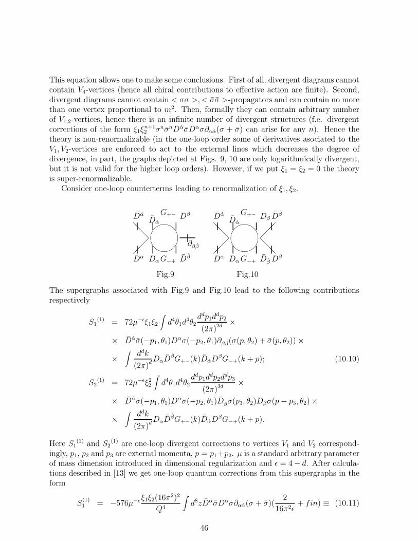
This equation allows one to make some conclusions. First of all, divergent diagrams cannotcontain V4-vertices (hence all chiral contributions to effective action are finite). Second,divergent diagrams cannot contain < σσ >,< σσ >-propagators and can contain no morethan one vertex proportional to m2. Then, formally they can contain arbitrary numberof V1,2-vertices, hence there is an infinite number of divergent structures (f.e. divergentcorrections of the form ξ1ξ

n+12 σnσnDασDασ∂αα(σ + σ) can arise for any n). Hence the

theory is non-renormalizable (in the one-loop order some of derivatives asociated to theV1, V2-vertices are enforced to act to the external lines which decreases the degree ofdivergence, in part, the graphs depicted at Figs. 9, 10 are only logarithmically divergent,but it is not valid for the higher loop orders). However, if we put ξ1 = ξ2 = 0 the theoryis super-renormalizable.

Consider one-loop counterterms leading to renormalization of ξ1, ξ2.

&%'$

Dα

Dα

@@@

Dα

Dα

∂ββ

Dβ

Dβ

G+−

G−+

Fig.9

&%'$

@@@

@@@

Dα

Dα

Dβ

Dβ

Dα

DαDβ

Dβ

G+−

G−+

Fig.10

The supergraphs associated with Fig.9 and Fig.10 lead to the following contributionsrespectively

S1(1) = 72µ−ǫξ1ξ2

∫

d4θ1d4θ2

ddp1ddp2

(2π)2d×

× Dασ(−p1, θ1)Dασ(−p2, θ1)∂ββ(σ(p, θ2) + σ(p, θ2)) ×

×∫

ddk

(2π)dDαD

βG+−(k)DαDβG−+(k + p); (10.10)

S2(1) = 72µ−ǫξ2

2

∫

d4θ1d4θ2

ddp1ddp2d

dp3

(2π)3d ×

× Dασ(−p1, θ1)Dασ(−p2, θ1)Dβσ(p3, θ2)Dβσ(p− p3, θ2) ×

×∫

ddk

(2π)dDαD

βG+−(k)DαDβG−+(k + p).

Here S1(1) and S2

(1) are one-loop divergent corrections to vertices V1 and V2 correspond-ingly, p1, p2 and p3 are external momenta, p = p1+p2. µ is a standard arbitrary parameterof mass dimension introduced in dimensional regularization and ǫ = 4− d. After calcula-tions described in [13] we get one-loop quantum corrections from this supergraphs in theform

S(1)1 = −576µ−ǫ ξ1ξ2(16π2)2

Q4

∫

d8zDασDασ∂αα(σ + σ)(2

16π2ǫ+ fin) ≡ (10.11)

46

≡ S(1)1div

+ S(1)1fin

;

S(1)2 = −576µ−ǫ ξ

22(16π2)2

Q4

∫

d8zDασDασDασDασ(2

16π2ǫ+ fin) ≡

≡ S(1)2div

+ S(1)2fin

.

In order to renormalize the theory we introduce the one-loop counterterms−S(1)

1 div, −S(1)2 div. It corresponds to the following renormalization transformation

Q2(0) = µ−ǫZQQ

2;

ξ1(0) = µ−ǫZ1ξ1; (10.12)

ξ2(0) = µ−ǫZ2ξ2

where Q2(0), ξ1(0), ξ2(0) are the bare parameters and Q2, ξ1, ξ2 are the renormalized ones. As

a result one obtains

Z1 = Z2 = (1 +72ξ2(16π)2

Q4ǫ). (10.13)

We see that in one-loop approximation there is the same independent renormalizationconstant both for ξ1 and ξ2. It means in particular that if we put ξ

(0)2 = cξ

(0)1 , where c is a

constant, then the renormalized parameters ξ1 and ξ2 will satisfy the same relation ξ2 =cξ1. One-loop renormalization does not destroy the relationship between the parametersin lower order.

Next step is a calculation of ZQ. Let us consider the supergraph given on Fig.11 (notethat we considered such a supergraph in Section 3)

&%'$

∂αα

∂ββ

Dα

DαDβ

DβG+−

G−+

Fig.11

The corresponding contribution looks like this

S(1)Q = −18µ−ǫξ2

1

∫

d4θ1d4θ2

∫ ddp

(2π)d∂ββσ(−p, θ1)∂αασ(p, θ2) × (10.14)

×∫ ddk

(2π)dDβDαD2D2

16δ12

DβDαD2D2

16δ12G2(k)G2(k + p).

Carrying out the transformations analogous to those used above we obtain

S(1)Q = −µ−ǫ

∫

d4θddx∂αασ∂αασ(

18ξ21(4π)4

Q4ǫ+ fin) ≡ S

(1)Qdiv

+ S(1)Qfin

. (10.15)

47

After introducing the one-loop counterterm −S(1)Q div

one will obtain using (10.12)

ZQ = (1 +32π2

Q2

18ξ21(4π)4

Q4ǫ). (10.16)

So we have studied renormalization of ξ1, ξ2 and Q2. As for the Λ, it was alreadynoted that all diagrams containing vertex of type V4 are finite, it means that the couplingΛ is not renormalized.

Now it remains to investigate renormalization of m2. It follows from (10.9), thatdivergent diagrams can contain no more than one vertex of V3-type corresponding tocoupling constant m2. All other possible vertices should be of V1- or V2-types.

We will study the divergent corrections to m2 in the case when ξ1= ξ2 = 0. It meansthat the vertices V1 and V2 are absent at all. It will be proved further that this casecorresponds to infrared limit of the theory. It means that only V3-type vertex can bepresented in the diagrams giving contribution to divergent correction to m2. All thesediagrams contain only one vertex V3-type, one internal line G+−-type and an arbitrarynumber of external lines corresponding to σ, σ

&%'$

@@@

... G+−

Fig.12

Let us consider such a diagram with a given number N of external lines, l from thoseare chiral and other are antichiral. Contribution of this diagram has the form

−m2

2

∫

d8zσl(z)σN−l(z)

l!(N − l)!G+−(z, z). (10.17)

Sum of all these contributions is equal to

S3 = −m2

2

∫

d8z∞∑

N=0

N∑

l=0

σl(z)σN−l(z)

l!(N − l)!G+−(z, z) =

m2

2

∫

d8zeσ+σG+−(z, z). (10.18)

In momentum representation the S3 can be written as follows

S3 = −m2

2

∫

d4θddxeσ+σ∫

ddk

(2π)d−A2k2 +m2

k2(−A2k2 +m2)2 − 81ΛΛ

D21D

21

16δ11. (10.19)

Taking into accountD2

1D21

16δ11 =

D21D

21

16δ12|θ1=θ2

= 1 (note that here the tadpole graphdepicted at Fig. 13 has the non-zero contribution!) we get

S3 = −m2

2

∫

d4θddxeσ+σ∫

ddk

(2π)d−A2k2 +m2

k2(−A2k2 +m2)2 − 81ΛΛ. (10.20)

48

After integration over momentum we get

S3 =m2

2

∫

ddxd4θeσ+σ(2

16π2A2ǫ+ fin).

We note that despite these diagrams are tadpole-type, their contribution is not equal tozero unlike Wess-Zumino model.

To cancel the divergence we should introduce a counterterm −S3div. It corresponds tomass renormalization

m20 = µ−ǫZmm

2;

Zm2 = 1 +2

16π2A2ǫ= 1 +

2

Q2ǫ(10.21)

Here m20 is a bare mass and m2 is a renormalized one.

Next step is consideration of beta functions. As usual, beta function for any renor-malized parameter g(µ) is defined as

βg = µdg

dµ,

where the renormalized parameter is expressed in term of the bare one g0 which does notdepend on µ, dg0

dµ= 0.

Using (10.13,10.12,10.21) we obtain the following beta functions

βξ1 =72(16π)2

Q4ξ1ξ2; βξ2 =

72(16π)2

Q4ξ22 ; βQ2 = 32π218(16π)2ξ2

1

Q4. (10.22)

As a result the equations for running couplings have the form

dξ1dt

= aξ1ξ2Q4

;dξ2dt

= aξ22

Q4;dQ2

dt= b

ξ21

Q4, (10.23)

where a = 21132π2, b = 32214π4. The solutions of these equations are

ξ1(t) =ξ1ξ2ξ2(t)

Q2(t) = Q2 + 8π2 ξ21

ξ22

(ξ2(t) − ξ2)

t =1

21132π2

− [Q2 − 8π2 ξ21

ξ22

](1

ξ2(t)− 1

ξ2) −

− 16π2(ξ1ξ2

)2

[Q2 − 8π2 ξ21

ξ22

] lnξ2(t)

ξ2+ (10.24)

+ 64π4(ξ1ξ2

)4

(ξ2(t) − ξ2)

.

Let us investigate the behaviour of running couplings ξ1(t), ξ2(t) and Q2(t) in infrareddomain when t → −∞. It is easy to see that in this case ξ2(t) → 0 and hence ξ1(t) → 0.

49

It means that ξ(0)1 = ξ

(0)2 = 0 is an infrared fixed point. For Q2(t) we obtain Q2(t) →

Q2 − 8π2 ξ21

ξ2. If we take quantities of initial ξ1 and ξ2 so that they correspond to infrared

fixed point ξ1 = ξ2 = 0 one gets Q2(t) → Q2. In particular, only the diagrams given onFig.4 can contribute to mass renormalization in infrared limit.

To investigate a behaviour of running mass we should use a notion of scaling dimensionof superfields. We note that the action of the theory (10.3) at ξ1 = ξ2 = 0 is invariantunder the transformations

δσ = (xa∂a +1

2θαDα)σ + 1; (10.25)

δσ = (xa∂a +1

2θαD

α)σ + 1

Let V be is some function depending on superfields σ, σ and their derivatives ∂aσ,∂aσ, Dασ, Dασ,. . . . We call that V has the scaling dimension ∆ if the transformationlaw of V under transformations (10.25) looks like this

δV [σ, σ] = (xa∂a +1

2θαDα +

1

2θαD

α + ∆)V. (10.26)

It is easy to see that the superfields σ, σ have no definite scaling dimension, thederivatives ∂aσ, ∂aσ have scaling dimension equal to 1, the spinor derivatives Dασ,Dασhave no definite scaling dimensions. However, the functions eσ, eσ have definite scalingdimensions ∆=1.

Let us fulfil the transformations σ → ασ, σ → ασ and S → 1α2S in the action (10.3)

at ξ1 = ξ2 = 0. It leads to the following action depending on arbitrary real parameter α

S =∫

d8z(−1

2

Q2

16π2σ2σ − m2

2α2eα(σ+σ)) + (

Λ

α2

∫

d6ze3ασ + h.c.).

We consider the calculation of the renormalization constant Zm in the theory (10.27).The only modification in comparison with eq. (10.21) is that we should use the propa-gator α2G+− in supergraph given by Fig.4. The parameter α is resulted here because ofexpansion of eα(σ+σ). It leads immediately to

Zm2 = 1 +2α2

Q2ǫ

Therefore the equation for running mass will be

dm2(t)

dt=

2α2m2(t)

Q2+ ∆m2m2(t). (10.27)

where ∆m2 is a scaling dimension of m2(t).To find ∆m2 we consider the term m2

2α2 eα(σ+σ) in the action (10.27). The scaling dimen-

sion of this term is −2, α is dimensionless and scaling dimension of eα(σ+σ) is 2α. Hence∆m2 = 2 − 2α. Therefore the equation (10.27) looks like this

dm2(t)

dt= (2 − 2α +

2α2

Q2)m2(t); (10.28)

m2(0) = m2

50

where we took into account that Q2(t) = Q2 in infrared limit. A solution of this equationcan be written in the form

m2(t) = m2 exp((2 − 2α +2α2

Q2)t). (10.29)

It is evident that at 2 − 2α + 2α2

Q2 > 0 we get m2(t) → 0 in infrared limit (note that

this condition is satisfied at α = 1, i.e. when there is no rescaling). It corresponds toκ2(t) → ∞ where κ2(t) is the running gravitational constant.

As for coupling constant Λ, its beta-function is equal to zero since the vertex of V4-typeis always finite (see above) and the fields σ, σ are not renormalized in this approach.

Therefore in infrared limit we stay with the following action

S =∫

d8z(−1

2

Q2

16π2σ2σ + (Λ

∫

d6ze3σ + h.c.). (10.30)

Our aim consists of calculation of low-energy leading contributions to one-loop effectiveaction. As usual, the first step is background-quantum splitting

σ → σ + χ, σ → σ + χ. (10.31)

Here σ, σ are background superfields, and χ, χ are quantum ones. It is known that to findone-loop contribution to effective action it is enough to consider the quadratic action ofquantum superfields which has the form

S(2)q [σ, σ;χ, χ] =

∫

d8z(−1

2

Q2

16π2χ2χ + (

9

2Λ∫

d6ze3σχ2 + h.c.).

The one-loop effective action Γ(1)[σ, σ] can be read off from expression

exp(iΓ1[σ, σ]) =∫

DχDχ exp(iS(2)q [σ, σ;χ, χ]). (10.32)

We suggest that the effective action, as usual, has the structure described by (9.2,9.3).The one-loop effective action in this theory can be expressed in the form of effectiveaction of some real scalar superfield just as we done in Wess-Zumino model: we considerthe theory of a real superfield v with action

Sv =Q2

16π2

1

16

∫

d8zvDαD2Dα2v. (10.33)

One-loop effective action Wv for this theory in the framework of Faddeev-Popov approachis given by

eiWv =∫

Dv exp(iSv)δ(1

4D2v − χ)δ(

1

4D2v − χ)∆, (10.34)

where ∆ is Faddeev-Popov determinant which is a constant as in Wess-Zumino model. Wenote that Wv is also a constant. After multiplying of left-hand side and right-hand side

51

of equations (10.32) and (10.34) respectively and integration over χ, χ we get one-loopcontribution to effective action Γ(1) in the form

Γ(1) = − i

2Tr log(

Q2

16π22

2 − 9Λe3σD2

4− 9Λe3σ

D2

4). (10.35)

In Schwinger representation the one-loop contribution to effective action looks like

Γ(1) = − i

2

∫ ∞

0

ds

sTr exp[is(

Q2

16π22

2 − 9Λe3σD2

4− 9Λe3σ

D2

4)]. (10.36)

After change s Q2

16π2 → s,Λ16π2

Q2 → Λ we can express this effective action as

Γ(1) = − i

2

∫ ∞

0

ds

sTreis2

2

exp[is(−9Λe3σD2

4− 9Λe3σ

D2

4)]. (10.37)

Really, commutators of 22 with background superfields can lead only to terms depending

on space-time derivatives of background superfields which lead only to higher orders in∂aσ. We can calculate exponent of ∆ = −9Λe3σ D

2

4− 9Λe3σ D

2

4by the same way as in

Wess-Zumino model. The necessary expressions are

eis22

δ4(x1 − x2)|x1=x2 =∫ d4k

(2π)4eisk

4

=1

32isπ2(10.38)

2eis22

δ4(x1 − x2)|x1=x2 =∫

d4k

(2π)4(−k2)eisk

4

= −√π

32π2(is)3/2. (10.39)

The expression (10.37) can be exactly found in two special cases:(i) kahlerian effective potential, in this case all derivatives of σ, σ are equal to zero.

The expression (10.37) is analogous to the expression (8.16) after redefinitions 9Λe3σ →ψ, 9Λe3σ → ψ. As a result we can easily restore expression for Schwinger coefficientsA(s), A(s) (6.9):

A(s) = A(s) =1

2[cosh(9isΛ

√e3(σ+σ)2) − 1]. (10.40)

The one-loop kahlerian effective potential is given by

K(1) = − i

2

∫ ∞

0[A(s) + A(s)]U(x, x′; s)|x=x′, (10.41)

where U(x, x′; s) = eis22δ4(x− x′). We can write

K(1) = − i

2

∫ ∞

0

ds

s

∞∑

n=0

[(9Λse32(σ+σ))2n+2

(2n+ 2)!2n]

eis22

δ4(x− x′)|x=x′. (10.42)

We can separate sum over n into sum over odd n and sum over even n. We use expressions(10.38) and take into account that

22neis2

2

δ4(x1 − x2) = (∂

∂is)neis2

2

δ4(x1 − x2) (10.43)

22n+1eis2

2

δ4(x1 − x2) = (∂

∂is)n2eis2

2

δ4(x1 − x2). (10.44)

52

As a result we find one-loop kahlerian effective potential in the form

K(1) = cΛ2/3(16π2

Q2)2/3eσ+σ, (10.45)

where c is a constant given in [38].(ii) chiral effective Lagrangian. To calculate it we put σ = 0 which leads to calculation

of

U(σ|s) = exp[is(−9Λe3σ)D2

4− 9Λ

D2

4)] (10.46)

up to the second (leading) order is spinor derivatives of σ. We note that as a resultone-loop effective action in leading order takes the form

Γ(1) =i

2

∫

d8z∫ ∞

0

ds

s[A1(σ|2)DασDασ + A2(σ|2)D2σ + A3(σ|2)] ×

× U0(x, x′; s)|x=x′. (10.47)

After transforming of this expression to the form of integral over d6z it is at least ofsecond order in space-time derivatives of σ. Hence we can put all coefficients A1, A2, A3

to depend only on σ but not on its derivatives. It means that at the step of calculatingU(σ|s) we can put all space-time derivatives of σ, σ to zero. After calculation of U(σ|s)(10.46) we get the coefficients of Schwinger expansion A(s), A(s) (note again that onlythey contribute to one-loop effective action, see (10.41)):

A(s) =1

2[cosh(iWs) − 1] (10.48)

A(s) = −16h(−8hφ(is)2 + 64h2

W 2(sinh(iWs)

W− is)D2φ+

+ 8192h4

W 5[iWs cosh(iWs) − 3 sinh(iWs) + 2iWs]DαφDαφ. (10.49)

Here φ = e3σ, h = −94Λ16π2

Q2 , W = 16he3/2σ√

2. This expression for A and A can be

substituted into (10.47). After expansion of A and A into power series, transformationof the contribution to the form of integral over d6z and integration over s (see details in[38]), one-loop leading chiral contribution to effective action takes the form

L(1)c = Λ1/3

[

(c1 + 3c3)e−σ + c2e

2σ + 3c4e−4σ∂mσ∂mσ + (c3e

−σ + c4e−4σ)2σ

]

. (10.50)

Here c1, c2, c3, c4 are finite constants given in [38]. We find that the leaing chiral contri-bution to effective action is of second order in space-time derivatives of chiral superfieldσ, therefore one-loop chiral effective potential is absent.

Then, if we sum classical action (10.3) and leading quantum corrections(10.45,10.50) we get one-loop corrected effective action. If we put in it all derivatives ofsuperfields to zero we get the following low-energy leading effective action:

Γ = c(Λ

Q2)2/3

∫

d8zeσ+σ + (Λ∫

d6ze3σ + h.c.). (10.51)

53

We remind that σ = log Φ, σ = log Φ where Φ, Φ are chiral and antichiral supergravityprepotentials (so called chiral compensators). Expression of this effective action in termsof Φ, Φ gives

Γ = c(Λ

Q2)2/3

∫

d8zΦΦ + (Λ∫

d6zΦ3 + h.c.). (10.52)

This action has the structure similar to the classical action of Wess-Zumino model. Hencewe see that Wess-Zumino model is generated at infrared limit of four-dimensional dilatonsupergravity.

11 Supergauge theories

This section is a brief review of results on supergauge theories. Unfortunately, restrictedvolume of this section does not allow to discuss all essential results of last years in thissphere hence we only give here main ones.

The starting point of our consideration is an action of N = 1 super-Yang-Mills theory:

SSYM =1

4g2

∫

d6ztrW αWα, (11.1)

where

Wα = −1

8D2(e−2gVDαe

2gV );V (z) = V I(z)T I . (11.2)

The V (z) = V I(z)T I is a real scalar Lie-algebra-valued superfield. We can expand theaction (11.1) into power series in coupling g. As a result we get

S =1

16

∫

d8ztr(V DαD2DαV + . . .). (11.3)

Here dots denote higher orders in g. The action (11.1) is invariant under gauge transfor-mations

e2gV → e−2igΛe2gV e2igΛ. (11.4)

where DαΛ = 0. The equivalent form of this transformation [10] is

δ(gV ) = LgV (2igΛ − 2igΛ + cothgV (2igΛ + 2igΛ)). (11.5)

Here LgVA = [gV, A] is a Lie derivative. It is easy to see that strengths Wα, Wα areinvariant under such transformations. The leading order in (11.5) is

δ(gV ) = 2ig(Λ − Λ). (11.6)

54

Since the theory is gauge invariant we must introduce gauge-fixing functions for quanti-zation. The most natural form of them is (cf. section 8 where these gauge-fixing functionswere used for calculation of one-loop effective action in Wess-Zumino model)

χ(V ) = −1

4D2V + f(z) (11.7)

χ(V ) = −1

4D2V + f(z).

Here f(z) is arbitrary chiral superfield. Variation of these gauge fixing functions undertransformations (11.5) is

δ

(

χ(V )χ(V )

)

=

(

0 −14D2

−14D2 0

)(

gΛgΛ

)

. (11.8)

According to Faddeev-Popov approach we can introduce the ghost action

SGH = c′δχ|gΛ=c,gΛ=c (11.9)

i.e. parameters of transformation gΛ, gΛ are ghosts. Here δχ ≡ δ

(

χ(V )χ(V )

)

. from (11.8),

c′ is a line (c′c′) and since Λ is chiral c, c′ are also chiral ones. Here c, c′ are chiral ghostsand c, c′ are antichiral ones. As usual, ghosts are fermions.

Therefore

SGH =∫

d6ztrc′δχ

δVδV +

∫

d6ztrc′δχ

δVδV, (11.10)

where

δV = LgV (c− c + cothgV (c+ c)). (11.11)

Therefore the action of ghosts looks like

SGH =∫

d8ztr(c′ + c′)LgV (c− c+ cothgV (c+ c)). (11.12)

Then, the generating functional for this theory at zero sources according to Faddeev-Popovapproach looks like

Z[J ]|J=0 =∫

DvDcei(SSY M+SGH)δ+(1

4D2V − f)δ−(

1

4D2V − f). (11.13)

Here Dc ≡ DcDc′DcDc′ We can average over functions f and f with weight

exp(i

ξ

∫

d8z(f f + bb)), (11.14)

where ξ is a some number (gauge parameter). The b, b are Nielsen-Kallosh ghosts (inthis case their contribution to effective action is a constant, but in background-covariantformulation it is non-trivial). As a result (11.13) takes the form

Z[J ]J=0 =∫

DvDcei(SSY M +SGH+SGF ), (11.15)

55

where

SGF =1

16ξ

∫

d8ztr(D2V )(D2V ) (11.16)

is a gauge-fixing action [10].We introduce the total action

Stotal = SSYM + SGF + SGH (11.17)

and the generating functional

Z[J, η] =∫

DVDc exp(i(Stotal +∫

d8ztrJV +∫

d6ztr(η′c′ + ηc) +

+∫

d6z(η′c′ + ηc))). (11.18)

Here η is the set of all sources: η, η′, η, η′. To develop diagram technique we must splitaction Stotal into free (quadratic) part and vertices. It is easy to see ([10, 39]) that

e−2gVDαe2gV = 2gDαV − 2g2[V,DαV ] +4

3[V, [V,DαV ]] + . . . . (11.19)

Therefore (11.1) looks like

SSYM =∫

d8ztr( 1

16V DαD2DαV +

1

8g(D2DαV )[V,DαV ] −

− 1

16g2[V,DαV ]D2[V,DαV ] − 1

12g2(D2DαV )[V, [V,DαV ]] + . . .

)

. (11.20)

And the ghost action is

SGH =∫

d8ztr(

c′c− cc′ + g(c′ + c′)[V, c− c] +g2

3(c′ + c′)[V, [V, c+ c]]

)

+ . . . . (11.21)

This expression is enough in one- and two-loop calculations.The quadratic action is

S0 =1

2

∫

d8ztrV(

− 2 +1

16(1 +

1

χD2, D2)

)

V +∫

d8ztr(c′c− cc′). (11.22)

Vertices can be read off from (11.20,11.21). Propagators look like

< V (z1)V (z2) > = − 1

2

(

− 1

82DαD2Dα + ξ

D2, D2162

)

δ8(z1 − z2) (11.23)

< c′(z1)c(z2) > = < c′(z1)c(z2) >=1

2δ8(z1 − z2).

We note that ghosts are fermions hence any ghost loop corresponds to minus sign. Then,D-factors are associated with vertices containing ghosts just by the same rule as with

56

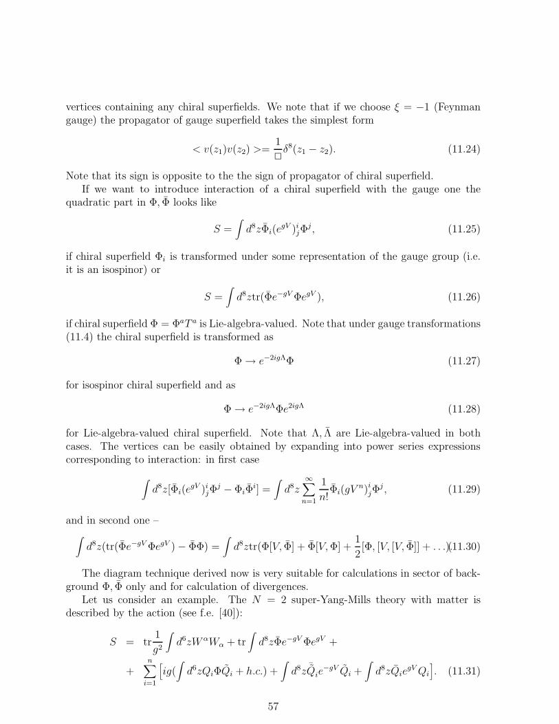
vertices containing any chiral superfields. We note that if we choose ξ = −1 (Feynmangauge) the propagator of gauge superfield takes the simplest form

< v(z1)v(z2) >=1

2δ8(z1 − z2). (11.24)

Note that its sign is opposite to the the sign of propagator of chiral superfield.If we want to introduce interaction of a chiral superfield with the gauge one the

quadratic part in Φ, Φ looks like

S =∫

d8zΦi(egV )ijΦ

j , (11.25)

if chiral superfield Φi is transformed under some representation of the gauge group (i.e.it is an isospinor) or

S =∫

d8ztr(Φe−gV ΦegV ), (11.26)

if chiral superfield Φ = ΦaT a is Lie-algebra-valued. Note that under gauge transformations(11.4) the chiral superfield is transformed as

Φ → e−2igΛΦ (11.27)

for isospinor chiral superfield and as

Φ → e−2igΛΦe2igΛ (11.28)

for Lie-algebra-valued chiral superfield. Note that Λ, Λ are Lie-algebra-valued in bothcases. The vertices can be easily obtained by expanding into power series expressionscorresponding to interaction: in first case

∫

d8z[Φi(egV )ijΦ

j − ΦiΦi] =

∫

d8z∞∑

n=1

1

n!Φi(gV

n)ijΦj , (11.29)

and in second one –∫

d8z(tr(Φe−gV ΦegV ) − ΦΦ) =∫

d8ztr(Φ[V, Φ] + Φ[V,Φ] +1

2[Φ, [V, [V, Φ]] + . . .).(11.30)

The diagram technique derived now is very suitable for calculations in sector of back-ground Φ, Φ only and for calculation of divergences.

Let us consider an example. The N = 2 super-Yang-Mills theory with matter isdescribed by the action (see f.e. [40]):

S = tr1

g2

∫

d6zW αWα + tr∫

d8zΦe−gV ΦegV +

+n∑

i=1

[

ig(∫

d6zQiΦQi + h.c.) +∫

d8z ¯Qie−gV Qi +

∫

d8zQiegVQi

]

. (11.31)

57

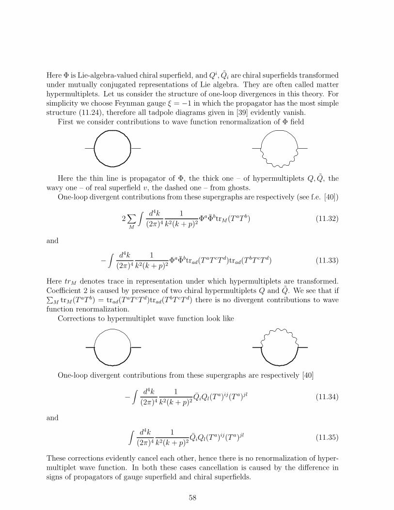
Here Φ is Lie-algebra-valued chiral superfield, andQi, Qi are chiral superfields transformedunder mutually conjugated representations of Lie algebra. They are often called matterhypermultiplets. Let us consider the structure of one-loop divergences in this theory. Forsimplicity we choose Feynman gauge ξ = −1 in which the propagator has the most simplestructure (11.24), therefore all tadpole diagrams given in [39] evidently vanish.

First we consider contributions to wave function renormalization of Φ field

Here the thin line is propagator of Φ, the thick one – of hypermultiplets Q, Q, thewavy one – of real superfield v, the dashed one – from ghosts.

One-loop divergent contributions from these supergraphs are respectively (see f.e. [40])

2∑

M

∫

d4k

(2π)4

1

k2(k + p)2ΦaΦbtrM(T aT b) (11.32)

and

−∫ d4k

(2π)4

1

k2(k + p)2ΦaΦbtrad(T

aT cT d)trad(TbT cT d) (11.33)

Here trM denotes trace in representation under which hypermultiplets are transformed.Coefficient 2 is caused by presence of two chiral hypermultiplets Q and Q. We see that if∑

M trM(T aT b) = trad(TaT cT d)trad(T

bT cT d) there is no divergent contributions to wavefunction renormalization.

Corrections to hypermultiplet wave function look like

One-loop divergent contributions from these supergraphs are respectively [40]

−∫

d4k

(2π)4

1

k2(k + p)2QiQl(T

a)ij(T a)jl (11.34)

and

∫

d4k

(2π)4

1

k2(k + p)2QiQl(T

a)ij(T a)jl (11.35)

These corrections evidently cancel each other, hence there is no renormalization of hyper-multiplet wave function. In both these cases cancellation is caused by the difference insigns of propagators of gauge superfield and chiral superfields.

58

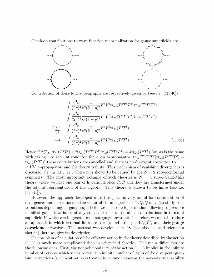
One-loop contributions to wave function renormalization for gauge superfields are

Contribution of these four supergraphs are respectively given by (see f.e. [41, 40])

∫

d4k

(2π)4

1

k2(k + p)2V aV btrad(T

aT cT d)trad(TbT cT d)

∫

d4k

(2π)4

1

k2(k + p)2V aV btrad(T

aT cT d)trad(TbT cT d)

2∑

M

∫

d4k

(2π)4

1

k2(k + p)2V aV btrM(T aT b)

−4∫

d4k

(2π)4

1

k2(k + p)2V aV btrM(T aT b). (11.36)

Hence if 2∑

M trM(T aT b) + 2trad(TaT cT d)trad(T

bT cT d) = 4trad(TaT b) (or, as is the same

with taking into account condition for < φφ >-propagator, trad(TaT cT d)trad(T

bT cT d) =trad(T

aT b)) these contributions are cancelled and there is no divergent correction to< V V >-propagator, and the theory is finite. This mechanism of vanishing divergences isdiscussed, f.e. in [41], [42], where it is shown to be caused by the N = 2 superconformalsymmetry. The most important example of such theories is N = 4 super-Yang-Millstheory where we have one pair of hypermultiplets Q, Q and they are transformed underthe adjoint representation of Lie algebra. This theory is known to be finite (see f.e.[39, 41]).

However, the approach developed until this place is very useful for consideration ofdivergences and corrections in the sector of chiral superfields Φ, Q, Q only. To study con-tributions depending on gauge superfields we must develop a method allowing to preservemanifest gauge invariance at any step as earlier we obtained contributions in terms ofsuperfield V which are in general case not gauge invariant. Therefore we must introducean approach in which external lines are background strengths Wα, Wα and their gauge

covariant derivatives. This method was developed in [28] (see also [44] and referencestherein), here we give its description.

The problem of calculation of the effective action in the theory described by the action(11.1) is much more complicated than in other field theories. The main difficulties arethe following ones. First, the nonpolynomiality of the action (11.1) implies in the infinitenumber of vertices which seems to result in infinite number of types of the divergent quan-tum corrections (such a situation is treated in common cases as the non-renormalizability

59

of the theory), second, it is easy to see that the common background-quantum splittingV → V0 + v where V0 is a background field and v is a quantum field cannot providemanifest gauge covariance of the quantum corrections. Really, because of the nonpoly-nomiality of W α (11.2), to get a covariant quantum correction (which by definition mustbe expressed in terms of the strengths Wα, Wα which are the only objects transformingcovariantly under the gauge transformations unlike of the superfield V itself) we need tosummarize an infinite number of supergraphs with different numbers of external V0 legs.The background field method provides an effective solution for both these problems.

The starting point of the method under discussion is a nonlinear background-quantumsplitting for the superfield V defining the action (11.1) [28]:

e2gV → e2gΩe2gve2gΩ. (11.37)

Here the v is a quantum field, the Ω, Ω are the background superfields (they are notnecessary chiral/antichiral ones). After such a background-quantum splitting, the classicalaction (11.1) takes the form:

S = − 1

64g2

∫

d8z(e−2gvDαe2gv)D2(e−2gvDαe2gv), (11.38)

In this expression (which describes a theory of real scalar superfield v coupled to back-ground superfields Ω, Ω) the Dα, Dα are the background covariant derivatives defined bythe expressions [41, 28]:

Dα = e−2gΩDαe2gΩ,

Dα = e2gΩDαe−2gΩ. (11.39)

Our further aim consists in study of the action (11.38). To do it let us first describethe properties of the background covariant derivatives given by (11.39). The Dα, Dα

in (11.39) act on all on the right. Then, as well as the covariant derivatives in usualdifferential geometry, the background covariant derivatives Dα, Dα can be represented inthe following “standard” form

Dα = Dα − iΓα, Dα = Dα − iΓα, (11.40)

where

Γα = ie−2gΩ(Dαe2gΩ), Γα = ie2gΩ(Dαe−2gΩ) (11.41)

are the superfield connections.Let us study the (anti)commutation relations for the Dα, Dα. We start with imposing

the following constraint

Dαα = − i

2Dα, Dα (11.42)

60

which represent itself as a background covariant analog of the common anticommutationrelation ∂αα = − i

2Dα, Dα. Then, it is easy to verify straightforwardly the following

definition of the background strength Wα (cf. [43]):

Wα = − i√2[Dα, Dα,Dα] =

√2[Dα,Dαα]. (11.43)

Really, after we substitute expressions (11.39) for the background-covariant derivatives to(11.43) and take into account that e2gΩe2gΩ = e2gV in the case of absence of the quantumfield v (cf. (11.37)) we get just the definition (11.2).

The relation (11.43) is crucial. Its treating consists of the fact that the background-covariant space-time derivative Dαα has non-zero commutators with spinor background-covariant derivatives unlike of the common covariant derivatives, and, moreover, thatthe background strengths could arise during the D-algebra transformations. In part, theidentity (11.43) implies in the following expressions [44]:

[Dα, D2] = 4i(−√

2W α + DαDαα) =

= 4i(√

2W α + DααDα). (11.44)

Another consequence of (11.43), and consequently of (11.44), is

−1

8DαD2Dα +

1

16D2, D2 = 2 − i

2W αDα −

i

2W αDα. (11.45)

This expression is a gauge covariant analog of the known relation−1

8DαD2Dα + 1

16D2, D2 = 2.

Basing on (11.43), we also can prove the following important relations:

D2D2D2 = 16(2 − i

2W αDα −

i

4(DαWα))D2 ≡ 162−D2;

D2D2D2 = 16(2 − i

2W αDα −

i

4(DαWα))D2 ≡ 162−D2. (11.46)

We also need in definition of the (background) covariantly chiral superfields to describecoupling of the gauge superfields to the matter. By definition, the superfield Φ is referredas the (background) covariantly chiral one if it satisfies the condition DαΦ = 0. It is easyto see that the Φ is related to the common chiral field Φ0 as

Φ = egΩΦ0. (11.47)

Really, condition of chirality DαΦ0 = 0 implies in

egΩDαe−gΩegΩΦ0 = 0. (11.48)

Using the definitions (11.39,11.47) we arrive just to the condition DαΦ = 0.Now we are in position to develop the petrurbative approach for the theory with

action (11.38). First, we note that this theory possesses the symmetry with respect tothe following gauge transformations:

egv → eigΛegve−igΛ (11.49)

61

where Λ is a covariantly chiral parameter, i.e. it satisfies the condition DαΛ = 0 (sim-ilarly, DαΛ = 0). Therefore we need to introduce a gauge fixing. The most naturalbackground covariant gauge fixing term looks like

Sgf = − 1

16

∫

d8zvD2, D2v (11.50)

which is a covariant generalization of the common gauge fixing term in the Feynmangauge. Summarizing the (11.38) and (11.50) and taking into account (11.45) we get thefollowing action of the quantum v field:

St = S + Sgf = −1

2

∫

d8zv2v + Sint. (11.51)

In principle, one can fix other gauges (by putting the factor ξ−1 in Sgf ), however, evenproblem of finding the propagator for v field appears to be very complicated (up to thistime nobody found this propagator in a closed form). Hence the Feynman gauge is themost convenient one. The propagator of the v field in the Feynman gauge is

< v(z1)v(z2) >= 2−1δ8(z1 − z2) (11.52)

(for the sake of the uniqueness of the consideration we relate all terms involving Wα, Wα

to the interaction part).The Sint in the expression above is an interaction part. It involves both covariant

generalizations of the “common” vertices and the new vertices involving the backgroundstrengths Wα, Wα manifestly:

Sint =∫

d8z(

v(− i

2W αDα −

i

2W αDα)v +

+1

8gvDαv, D2Dαv +

1

3[[Dαv, v], v]iWα − (11.53)

− 1

16g2[v,Dαv]D2[v,Dαv] −

1

12g2D2Dαv[v, [v,Dαv]] +

1

6[[[Dαv, v], v], v]iWα

)

+ . . . .

Because of the gauge symmetry, one needs to introduce ghosts. Since the form of thegauge transformations and gauge fixing action is very similar to the “common” super-field case with only difference consisting in covariant chirality instead of common one,the action of ghosts in this case also will be analogous to the common case with onlydifference consisting in the fact of the covariant chirality of the ghosts c, c′ or covariant

antichirality of the ghosts c, c′:

Sgh =∫

d8z(c′ + c′)Lgv(c− c+ cthLgv(c+ c)) (11.54)

which after expansion in the power series gives:

Sgh =∫

d8z(c′c− cc′ + (c′ + c′)[v, c+ c]) +1

12(c′ + c′)[v, [v, c+ c]] + . . .). (11.55)

62

The action of the matter after the background-quantum splitting of the gauge fields takesthe form

Sm =∫

d8zΦegvΦ, (11.56)

where Φ, Φ are the covariantly chiral and antichiral superfields. The propagators ofchiral superfields and ghosts are

< φφ >= − 1

16D2

2−1+ D2, < c′c >=< cc′ >== − 1

16D2

2−1+ D2. (11.57)

We note that such propagators can be expanded into power series in Wα, Wα, see (11.46).The expressions (11.53,11.55,11.56,11.52,11.57) can be used for constructing the super-graphs. The examples of application of the method for the supergraph calculations canbe found in [44].

Now let us give a comparative characteristics for the two methods of superfield calcu-lations – the background field method and the “common” method.

The crucial difference is the following one. In the framework of the “common” methodthe quadratic and linear divergences could arise for the supergraph with arbitrary anynumber of the external legs. Really, it is easy to show that the superficial degree ofdivergence for the “common” supergraph is

ω = 2 − 1

2ND −Eφ, (11.58)

where ND is a number of spinor supercovariant derivatives associated to the external legs,Eφ is a number of external chiral (antichiral) legs. We note that the quadratic and/orlinear divergences are possible for any number of external v legs. At the same time, inthe framework of the background field method by the construction of the background-quantum splitting the only external lines are the background strengths and/or their co-variant derivatives. The superficial degree of divergence in this case can be shown to havethe form

ω = 2 − 3

2NW − 1

2ND + ǫ− Eφ, (11.59)

where NW is a number of the background strength legs, ǫ = 1 for the chiral (antichiral)contribution (which only possible structure is

∫

d6zW 2,∫

d6zW 2), otherwise ǫ = 0; theND is the number of derivatives acting on external Wα, Wα legs (the derivatives presentingin each Wα, Wα by definition must not be taken into account!). We see that in frameworkof this approach only logarithmic overall divergences are possible, they arise for the termsproportional to W 2, with the quadratic and linear subdivergences (which are importantif we make a noncommutative generalization) can arise only in subgraphs which are notassociated to the external Wα, Wα legs.

From formal viewpoint such a difference has the following origin. Really, the superfieldstrength by construction contains three spinor derivatives, hence arising of any superfieldstrength leg in the framework of “common” formalism decreases by three the number of

63

the D-factors which could be converted to momenta (we note that use of the backgroundfield method allows to sum automatically the infinite number of “common” graphs andforbids existence of the supergraphs with the superficial quadratic or linear divergence),as a result, the convergence of the supergraph is improved. It is essential in the non-commutative field theory since it means that the only problems could be generated bysubgraphs only as each contribution to the effective action is in worst case only logarith-mically divergent. In part, it means that there is no contradiction between the result ofBichl et al. [45] according to which the different contributions to the one-loop two-pointfunction of v field in the U(1) NC SYM theory possess quadratic divergences (only theirsum is free of dangerous UV/IR mixing) and the result of Zanon et al. [46] accordingto which all one-loop contributions to the effective action in the same theory are free ofthe dangerous UV/IR mixing (notice that the calculations in the last paper were carriedout in the framework of the background field method); we should mention also use ofthe background field method in the papers [46] devoted to study of the one-loop effectiveaction in the noncommutative super-Yang-Mills theories. We note that the backgroundfield method allows to preserve the gauge covariance at all steps of calculations.

However, the background field method has one disadvantage – presence of nontrivialcommutators of the covariant derivatives makes all calculations extremelly difficult fromthe technical viewpoint.

12 Conclusions

We considered superfield method in supersymmetric field theory. This method allows topreserve manifest supersymmetry at any step of calculations, and the calculations withinit turns to be much more compact than within the framework of the component approach.

We studied several examples of superfield theories and presented in details quantumcalculations for them. These examples were Wess-Zumino model, general chiral super-field model, dilaton supergravity and N = 1 super-Yang-Mills theory with chiral matter.In these theories we developed supergraph technique, studied general form of superfieldeffective action and calculated low-energy leading contributions to effective action. It isnatural to expect that development of superfield quantum calculations in other superfieldmodels formulated in terms of N = 1 superfields including different supergravity modelsis in principle no more difficult. We also discussed the background field method in thesupergrauge theories.

Let us briefly discuss other applications and generalizations of the superfield approachin the quantum field theory. In the last years the following most important ways ofapplications of superfield supersymmetry were developed.

1. Studying of theories with extended supersymmetry. It is known thattheories with extended supersymmetry possess better renormalization properties, f.e. asN = 1 super-Yang-Mills theory is renormalizable, the N = 4 super-Yang-Mills theory isfinite. The most important examples of theories with extended supersymmetry are N = 2and N = 4 super-Yang-Mills theories. During last years numerous results in studying ofthese theories were obtained (see f.e. [47, 48, 49] and references therein).

64

It is natural to expect that the most adequate method for consideration of such theoriesmust possess manifest N = 2 supersymmetry. Such a method is a harmonic superspaceapproach developed in [50],[51]. This method is based on consideration of superfields beingthe functions of bosonic space-time coordinates xa, two sets of Grassmann coordinatesθiα, θiα with i = 1, 2 and spherical harmonics u±i. Introducing of analytic superfield[50] allows to develop formulation in terms of unconstrained N = 2 superfield and toavoid arising of component fields with higher spins. The formulations of N = 2 andN = 4 super-Yang-Mills theories in harmonic superspace is given in [50, 51], backgroundfield method for these theories is developed in [52, 53, 54], and examples of quantumcalculations are given in [48, 49, 55, 56, 57]. The most important results presented inthese papers are calculation of holomorphic action of N = 2 matter hypermultipletsin external N = 2 gauge superfield, calculation of one-loop nonholomorphic effectivepotential in N = 4 super-Yang-Mills theory and proof of its absence in higher loops,calculation of one-loop effective action for N = 4 super-Yang-Mills theory for constantstrength tensor Fab, calculation of superconformal anomaly of N = 2 matter interactingwith N = 2 supergravity. During last years other important results achieved in theseinvestigations were calculation of contributions depending on derivatives of N = 2 super-Yang-Mills strength W [58, 59], calculation of contributions depending on backgroundmatter hypermultiplet fields [60], and development of quantum approach for N = 3super-Yang-Mills theory [61] (the manifestly N = 3 supersymmetric approach based onthe harmonic superspace technique for the N = 3 supersymmetric theory was given inpaper [62]).

2. Noncommutative supersymmetric theories. Noncommutative theories havebeen intensively studied during last years. Concept of space-time noncommutativity wasintroduced to quantum field theory due to some consequences of D-branes theory [63] andto consideration of quantum theories on very small distances where quantum fluctuationsof geometry are essential. Consideration of supersymmetric noncommutative theories isquite natural. During last years some interesting results in studying of noncommuta-tive supersymmetric theories were obtained but they were mostly based on componentapproach. The first superfield results were calculation of leading (∼ F 4) correction toone-loop effective action for N = 4 super-Yang-Mills theory [46] and formulation of su-pergraph technique for noncommutative Wess-Zumino model [64]. Further, the quantumsuperfield studies for the Wess-Zumino model [65] and four-dimensional superfield QED[66] and super-Yang-MIlls theories [67] were carried out. These theory were shown to beconsistent in the sense of absence of the nonintegrable UV/IR infrared divergences. Thus,we can speak about construction of the consistent noncommutative generalizations of thesupersymmetric theories of electromagnetic, strong and weak interactions. Therefore, thenext most important problem could consist in development of the noncommutative su-persymmetric generalization for the last fundamental interaction – the gravitational one.However, this problem is of course extremely difficult (see discussion of the problem f.e.in [68, 69]).

3. Noncommutative superspace. One more approach in the superfield quantumtheory is based on use of the noncommutative superspace [70]. Within it, the fermionicsuperspace coordinates form the Clifford algebra instead of the Grassmann algebra, which,

65

in part, leads to the modified construction of the Moyal product. In the framework of thisapproach, the generalizations of the Wess-Zumino (see f.e. [71] and reference therein),gauge (see f.e. [72] and reference therein) and general chiral superfield model [73] werestudied.

Then, there are a lot of applications of superfields approach to problems of supersym-metric quantum field theory (f.e. to studying of AdS/CFT correspondence which wascarried out mostly on base of component approach), and of course consideration of manyproblems originated from superstrings and branes theory.

As a final conclusion, we can suppose that superfield approach in quantum field theoryis a very perspective one, and there are a lot of ways for its development and moreapplications.

Acknowledgements. Author is grateful to Prof. V. O. Rivelles, Prof. M. O. C.Gomes, Prof. H. O. Girotti and Prof. A. J. da Silva for discussions and joint researches,to Prof. I. L. Buchbinder, Prof. M. Cvetic, Prof. S. M. Kuzenko for collaboration, andto Instituto de Fisica, Universidade de Sao Paulo and Instituto de Fisica, UniversidadeFederal do Rio Grande do Sul for hospitality. The work was supported by FAPESP,project No. 00/12671-7.

References

[1] M. Green, J. Schwarz, E. Witten. Theory of superstrings, Cambridge, UK: Univ.Pr., 1987, vol. 1-2.

[2] D. V. Volkov, V. P. Akulov. JETP Lett., 16, 621 (1972); Phys. Lett. B46, 109(1973).

[3] Y. A. Golfand, E. S. Lichtman. JETP Lett., 13, 323 (1971).

[4] J. Wess, B. Zumino. Nucl. Phys. B70, 139 (1974); Nucl. Phys. B78, 1 (1974).

[5] The Supersymmetric World, ed. by G. Kane and M. Shifman, World Scientific, 2000.

[6] J. Wess, B. Zumino. Phys. Lett. B49, 52 (1974).

[7] A. Salam, J. Strathdee. Nucl. Phys. B76, 477 (1974).

[8] S. Ferrara, J. Wess, B. Zumino. Phys. Lett. B51, 239 (1974).

[9] J. Wess, J. Bagger. Supersymmetry and supergravity. Princeton University Press,Princeton, 1983.

[10] I. L. Buchbinder, S. M. Kuzenko. Ideas and Methods of Supersymmetry and Super-gravity. IOP Publishing, Bristol and Philadelphia, 1998.

[11] V. Ogievetsky, L. Mezinchesku. Uspehi Fiz. Nauk (Phys. Sci. Achievments) 117,637 (1975) (in Russian).

66

[12] I. L. Buchbinder, A. Yu. Petrov. Yad. Fiz. (Phys. Atom. Nucl.) 63, 9, 2557 (2000).

[13] I. L. Buchbinder, A.Yu. Petrov. Class. Quant. Grav. 13, 2081 (1996).

[14] N. Seiberg, E. Witten. Nucl. Phys. B430, 19 (1994).

[15] P. West. Introduction to supersymmetry and supergravity. World Scientific, 1989.

[16] P. West. Phys. Lett. B258, 375 (1991).

[17] I. Jack, D. R. T. Jones. Problems of supersymmetric regularization, in: Kane G. L.(ed.), Perspectives of supersymmetry, 149-167 (hep-ph/9707278).

[18] J. Collins. Renormalization, UK: Univ. Pr., 1984.

[19] I. Jack, D. R. T. Jones, P. West. Phys. Lett. B258, 382 (1991).

[20] P. West. Phys. Lett. B261, 396 (1991).

[21] I. L. Buchbinder, S. M. Kuzenko, A.Yu. Petrov. Phys. Lett. B321, 372 (1994).

[22] I. L. Buchbinder, S. M. Kuzenko, A. Yu. Petrov. Yad. Fiz. (Phys. Atom. Nucl.), 59,1, 157 (1996).

[23] I. L. Buchbinder, S. D. Odintsov, I. L. Shapiro. Effective action in quantum gravity.IOP Publishing, Bristol and Philadelphia, 1992.

[24] B.S. De Witt. Dynamical theory of groups and fields. Princeton Univ. Press, Prince-ton, 1987.

[25] I. L. Buchbinder, S. M. Kuzenko, J. V. Yarevskaya. Nucl. Phys. B411, 665 (1994);Yad. Fiz. (Phys. Atom. Nucl), 56, 5, 202 (1993).

[26] I. N. McArthur, T. D. Gargett. Nucl. Phys. B497, 525 (1997).

[27] S. Coleman, S. Weinberg. Phys. Rev. D7, 1888 (1973).

[28] M. T. Grisaru, M. Rocek, W. Siegel. Nucl. Phys. B159, 429 (1979).

[29] A. Pickering, P. West. Phys. Lett. B353, 54 (1997).

[30] A. Yu. Petrov. Superfield effective action in supersymmetric field theories (PhDthesis), Tomsk, 1997.

[31] S.M. Kuzenko, J. V. Yarevskaya. Yad. Fiz. (Phys. Atom. Nucl.) 56, 5, 195 (1993).

[32] G. Cleaver, M. Cvetic, J.R. Espinosa, L. Everett, and P. Langacker, Nucl. Phys.B525, 3, 1998; Phys. Rev, D59, 115003, 1999; M. Cvetic, L. Everett, and J. Wang.Nucl. Phys. B538, 52 (1999).

67

[33] A.Yu. Petrov. Effective action in general chiral superfield model, Preprint hep-th/0002013.

[34] I. L. Buchbinder, A.Yu. Petrov. Phys.Lett. B461, 209 (1999).

[35] K. Symanzik. Commun. Math. Phys, 34, 7 (1973); T. Appelquist and J. Carrazone,Phys. Rev. D11, 2856 (1975).

[36] I. L. Buchbinder, M. Cvetic, A.Yu. Petrov. Mod.Phys. Lett. A15, 783 (2000); Nucl.Phys. B571, 358 (2000).

[37] I. L. Buchbinder, S. M. Kuzenko. Phys. Lett. B202, 233 (1988).

[38] I. L. Buchbinder, A. Yu. Petrov. Class. Quant. Grav. 14, 21 (1997).

[39] S. Kovacs. A perturbative reanalysis of N = 4 supersymmetric Yang-Mills theory,Preprint hep-th/9902047.

[40] A. De Giovanni, M. T. Grisaru, D. Zanon. Phys. Lett. B409, 251 (1997).

[41] S. J. Gates, M. T. Grisaru, M. Rocek, W. Siegel. Superspace or One Thousand andOne Lectures in Supersymmetry, Benjamin/Cummings, 1983.

[42] P. S. Howe, K. Stelle, P. West. Phys. Lett. B124, 55 (1983).

[43] M. T. Grisaru, W. Siegel, Nucl. Phys. B201, 292 (1982).

[44] M. T. Grisaru, D. Zanon, Phys. Lett. B142, 359 (1984); Nucl. Phys. B252, 578(1985).

[45] A. A. Bichl, M. Ertl, A. Gerhold, J. M. Grimstrup, H. Grosse, L. Popp, V. Putz,M. Schweda, R. Wulkenhaar. Int. J. Mod. Phys. A19, 4231 (2004).

[46] D. Zanon, Phys. Lett. B502, 265 (2001), Phys. Lett. B504, 101 (2001); A. Santam-brogio, D. Zanon, JHEP 0101, 024 (2001); M. Pernici, A. Santambrogio, D. Zanon,Phys. Lett. B504, 131 (2001).

[47] I. L. Buchbinder, S. M. Kuzenko, A.A. Tseytlin. Phys. Rev. D62, 045001 (2000).

[48] I. L. Buchbinder, S. M. Kuzenko. Phys. Lett. B446, 216 (1999); Mod. Phys. Lett.A13, 1623 (1998).

[49] I. L. Buchbinder, A. Yu. Petrov. Phys. Lett. B469, 482 (2000).

[50] A. Galperin, E.Ivanov, S. Kalitzin, V. Ogievetsky, E. Sokachev. Class. Quant. Grav.1, 469 (1984).

[51] A. Galperin, E. Ivanov, V. Ogievetsky, E. Sokachev. Class. Quant. Grav. 2, 601(1985); 2, 617 (1985).

68

[52] E.I. Buchbinder, I. L. Buchbinder, E. A. Ivanov, S. M. Kuzenko, B. A. Ovrut. Phys.Lett. B412, 309 (1997).

[53] E. I. Buchbinder, I. L. Buchbinder, S. M. Kuzenko, B. A. Ovrut. Phys. Lett. B417,61 (1997).

[54] I. L. Buchbinder, S. M. Kuzenko, B. A. Ovrut. Phys. Lett. B433, 335 (1997).

[55] I. L. Buchbinder, I. B. Samsonov. Mod. Phys. Lett. A14, 2537 (1999).

[56] S. M. Kuzenko, I. N. McArthur. Phys. Lett. B506, 140 (2001).

[57] S. M. Kuzenko, S. Theisen. Class. Quant. Grav. 17, 665 (2000).

[58] I. L. Buchbinder, A. Yu. Petrov, A. A. Tseytlin, Nucl. Phys. B621, 179 (2002).

[59] S. M. Kuzenko, I. N. McArthur, JHEP 0310, 029 (2003); Nucl. Phys. B683, 3 (2004);Nucl. Phys. B697, 89 (2004).

[60] I. L. Buchbinder, E. A. Ivanov, A. Yu. Petrov, Nucl. Phys. B653, 64 (2003).

[61] I. L. Buchbinder, E. A. Ivanov, I. B. Samsonov, B. M. Zupnik, Nucl. Phys. B689,91 (2004).

[62] F. Delduc, I. McCabe. Class. Quant. Grav. 6, 233 (1989).

[63] N. Seiberg, E. Witten. JHEP 9909, 032 (1999).

[64] A. A. Bichl, J. M. Grimstrup, H. Grosse, L. Popp, M. Schweda, R. Wulkenhaar.JHEP 0010, 046 (2000).

[65] I. L. Buchbinder, M. Gomes, A. Yu. Petrov, V. O. Rivelles, Phys. Lett. B517, 191(2001).

[66] A. F. Ferrari, H. O. Girotti, M. Gomes, A. Yu. Petrov, A. A. Ribeiro, V. O. Rivelles,A. J. da Silva, Phys. Rev. D69, 025008 (2004).

[67] A. F. Ferrari, H. O. Girotti, M. Gomes, A. Yu. Petrov, A. A. Ribeiro, V. O. Rivelles,A. J. da Silva, Phys. Rev. D70, 085012 (2004).

[68] A. H. Chamseddine, J. Math. Phys. 44, 2534 (2003).

[69] M. A. Cardella, D. Zanon, Class. Quant. Grav. 20, L95 (2003).

[70] N. Seiberg, 0306, 010 (2003).

[71] M. T. Grisaru, S. Penati, A. Romagnoni, Class. Quant. Grav, S1391 (2004); A. T.Banin, I. L. Buchbinder, N. G. Pletnev, JHEP 0407, 011 (2004).

[72] S. Penati, A. Romagnoni, ”Covariant quantization of N = 1/2 SYM theory andsupergauge invariance”, Preprint hep-th/0412041.

69

[73] O. D. Azorkina, A. T. Banin, I. L. Buchbinder, N. G. Pletnev, ”Generic chiral su-perfield model on anticommutative N = 1/2 superspace”, Preprint hep-th/0502008.

70