quantum theory of securities price formation in financial markets
TRANSCRIPT

1
Quantum theory of securities price formation in financial markets
(with application to spread and return probability distribution modeling)
Jack Sarkissian
Managing Member, Algostox Trading
email: [email protected]
Abstract
We develop a theory of securities price formation and dynamics based on quantum approach without
presuming any similarities with quantum mechanics. Disorder introduced by trading environment leads to
probability distribution of returns that is not a smooth curve, but a speckle-pattern fluctuating in both
price coordinate and time. This means that any given return can at times acquire a substantial probability
of occurring while remaining low on average in time. Still, due to local character of order interaction
during price formation the distribution width grows smoothly, has a minimum value at small time scale
and behaves ∼ √𝑡 at large time scale. Examples of calibration to market data, both intraday and daily, are
provided.

2
1. Introduction
It is commonly accepted that security prices follow a diffusion process. That process can be free diffusion,
mean-reverting, with or without memory, but it’s always some form of diffusion. Accordingly, probability
distribution of returns obeys the diffusion equation, and for free diffusion its width scales as √𝑡 with time.
This theory works well for a large time scale and on liquid securities. Many financial institutions work
within this framework, applying it to making trade decisions, derivatives pricing, SLB1, and risk
management.
Picture is different at time scale that is as small as the typical time between transactions. Price uncertainty
stops scaling down and does not approach zero anymore. It stays at the value relevant enough for the
security [1-3] and cannot be reduced further. That value is represented by bid-ask spread of the order book.
Additionally, the return distribution substantially deviates from Gaussian and becomes more fat-tailed [4].
Clearly the diffusion theory breaks, and a new theory is needed that can relate to spread as its intrinsic
characteristic. That theory must have the diffusion theory as a limiting case for large time scale.
Let us specify some notions. In financial markets buying and selling orders are lined up on an
exchange, and the record of current orders is called an order book. An example of order book is
shown in Fig. (1). The trading parties wait in line for a matching order, and when such order arrives
a transaction is recorded. Until a transaction occurs there is no single price to the security. Instead,
there is a spectrum of prices, that potentially represents the price. Spread is the difference between
the lowest selling and highest buying prices:
Δ = 𝑠𝑎𝑠𝑘 − 𝑠𝑏𝑖𝑑, (1)
1 Securities lending and borrowing

3
where 𝑠𝑎𝑠𝑘 is the best “ask” and 𝑠𝑏𝑖𝑑 is the best “bid”. By its nature, spread represents the risk
premium that is supposed to cover price uncertainty during the liquidation period.
Bid Ask
Price Size Price Size
27.83 100 27.87 100
27.82 100 27.9 100
27.8 200 27.95 1000
27.79 600 28.15 300
27.78 100 28.2 400
Fig. 1. Sample order book.
Spread has been a subject of active research in recent years. The most common approach is to obtain it as
a result of modeling processes in the order book. Once order arrival, cancellation and execution are
adequately modeled, spread is obtained by direct calculation from Eq. (1) [5,6]. Another approach is to
obtain spread as the optimal value from market maker’s perspective [7,8]. This approach allows to calculate
spread from microstructural parameters, but also depends on the degree of market maker’s risk aversion.
We believe that theory of spread and price formation should begin with understanding the nature of price.
Security price as a specific number is not an object that exists continuously and independently. It exists
only when it is measured: at the time of transaction. Without a transaction, one can just say that the price is
locked between best bid and best ask prices. However, sometimes one of these prices may not exist. At
times both prices may not exist. We see that on microstructural level we can at best talk about price
localization in a certain region. Price uncertainty disappears only at the time of transaction. We can say that
every financial transaction is an elementary act of price measurement. Measurement leads to selection

4
out of the entire price spectrum according to probability of each price and probability of the security to be
found in the state with that price [9]. These considerations point to quantum nature of price formation.
Application of quantum mechanics to finance is not surprising: quantum mechanics is probabilistic, and so
are financial markets. A number of attempts has been made to describe price behavior with methods of
quantum mechanics [10-19]. Some of them map the known quantum mechanical solutions to finance, thus
relying on a postulate that quantum mechanics applies to finance unchanged. Others attempt to rederive
quantum equations as they apply to finance. Although these models yield results with characteristics of
financial markets, we feel that more evidence is needed for how well they describe the observed market
data and how well they can be calibrated and used in an institutional setting.
At large time scale Δ𝑡 ≫ 𝜏0, 𝜏0 being the average time between transactions, price variations are usually
much larger than the spread, and price spectrum as well as the trading process can be considered continuous.
At such time scale a valid theory of price formation must go back to stochastic framework and result in
~√𝑡 widening of probability distribution provided by the diffusion equation. Motivated by this argument,
some researchers see the solution in attempting to extract Schrodinger equation from the diffusion equation
[18]. We believe that stochastic framework should be obtained as a limiting case from quantum framework,
and not the other way around.
In this paper we further develop quantum framework originally proposed by us in [1]. In that work we
showed that the two-level quantum coupled-mode model adequately describes the statistics of spread and
mid-price. Further development of the model in [2] showed that the model is capable of explaining the
relationship between spread, trading volume and volatility. These results make this theory very promising.
Here we do not pursue strict mathematical completeness, rather we are concerned with building analytical
base corresponding to the nature of processes and useful in practical applications.
We will refer to “spread” as a broader concept that can be defined in different ways for different levels of
data specification. For example, if the data represents an instantaneous snapshot of order book then the

5
spread is literally the difference between the best offer and the best bid in the book. We can also consider
the spread to be the difference between the effective offer and effective bid prices, which are represented
by order weighted averages of top 𝑁 levels of order book. Lastly, if the data is represented by OHLC2 time
series, one can consider the spread to be the difference between high and low prices. These notions are
formulated more accurately in [1].
For simplicity, but without loss of generality, we will discuss only equities here (stocks). Similar
considerations are applicable to other asset classes, such as fixed income, currency, commodities, and
futures.
2. Price operator and evolution equation
Price operator and its properties
The basic element of our approach is the probability amplitude 𝜓, which describes the state of the security,
and whose absolute value squared represents the probability of finding the security in the given state:
𝑝 = |𝜓|2 (2)
Security prices are governed by the price operator �̂�. Price operator’s eigenfunctions represent the pure
states in which the security can be found, and eigenvalues represent the spectrum of prices that the security
can attain in each corresponding state with quantum number 𝑛:
�̂�𝜓𝑛 = 𝑠𝑛𝜓𝑛 (3)
2 OHLC are the traditional open-high-low-close bars

6
To guarantee that prices are real numbers the price operator �̂� must be Hermitian. Price spectrum is
determined by the following equation
det‖𝑠𝑚𝑛 − 𝑠𝑛𝛿𝑚𝑛‖ = 0 (4)
Matrix elements of the price operator fluctuate in time, which introduces random properties to
eigenvalues and eigenfunctions:
�̂�(𝑡 + 𝛿𝑡) = �̂�(𝑡) + 𝛿�̂�(𝑡) (5)
and therefore:
𝑠𝑛(𝑡 + 𝛿𝑡) = 𝑠𝑛(𝑡) + 𝛿𝑠𝑛(𝑡) (6)
For a two-level system Eq. (3) takes the following form:
𝜓 = (
𝜓𝑎𝑠𝑘
𝜓𝑏𝑖𝑑) and (
𝑠11 𝑠12
𝑠12∗ 𝑠22
) (𝜓𝑎𝑠𝑘
𝜓𝑏𝑖𝑑) = 𝑠𝑎𝑠𝑘/𝑏𝑖𝑑 (
𝜓𝑎𝑠𝑘
𝜓𝑏𝑖𝑑) (7)
Given this, the bid and ask prices can be obtained as
𝑠𝑎𝑠𝑘 = 𝑠𝑚𝑖𝑑 +Δ
2 and 𝑠𝑏𝑖𝑑 = 𝑠𝑚𝑖𝑑 −
Δ
2 (8a)
𝑠𝑚𝑖𝑑 =
𝑠11 + 𝑠22
2=
𝑠𝑏𝑖𝑑 + 𝑠𝑎𝑠𝑘
2(mid − price) (8b)
Δ = √(𝑠11 − 𝑠22)2 + 4|𝑠12|2(spread) (8c)
The fluctuating matrix elements 𝑠𝑖𝑘 of price operator can be parametrized as follows:
𝑠11(𝑡 + 𝑑𝑡) = 𝑠𝑚𝑖𝑑(𝑡) + 𝜎𝑑𝑧 +
𝜉
2 (9a)

7
𝑠22(𝑡 + 𝑑𝑡) = 𝑠𝑚𝑖𝑑(𝑡) + 𝜎𝑑𝑧 −
𝜉
2 (9b)
𝑠12(𝑡 + 𝑑𝑡) =𝜅
2 (9c)
where 𝑑𝑧 ∼ 𝑁(0,1), 𝜉~𝑁(𝜉0, 𝜉1) and 𝜅~𝑁(𝜅0, 𝜅1). In such setup the mid-price and the spread are
given by equations:
𝑠𝑚𝑖𝑑(𝑡 + 𝑑𝑡) = 𝑠𝑚𝑖𝑑(𝑡) + 𝜎𝑑𝑧 (10a)
Δ = √𝜉2 + 𝜅2 (10b)
As we can see, the mid-price simply follows a Gaussian process with volatility 𝜎. Spread, on the
other hand, behaves as quantum-chaotic quantity [1, 20], whose statistics matches the observed
spread statistics quite well both on bid-ask micro-level and on bar data level, see Figs. 2a, 2b.
Fig. 2a. Calibration of Coupled-Wave Model to bid-ask data for AAPL and AMZN, [1]
AAPL AMZN

8
Fig 2b. Calibration of Coupled-Wave Model to bar data for AAPL and AMZN, [1]
Price dynamics
Evolution equation for the probability amplitude can be obtained from the following consideration. Total
probability is conserved and equal to one at all times:
∑|𝜓𝑛|2 = 1
𝑛
(11)
Then, differentiating this in 𝑡:
∑(𝜓𝑛
∗𝜕𝜓𝑛
𝜕𝑡+ 𝜓𝑛
𝜕𝜓𝑛∗
𝜕𝑡)
𝑛
= 0 (12)
The most general linear equation satisfying this condition is3:
𝑖𝜏𝑠
𝜕𝜓
𝜕𝑡= �̂�𝜓 (13)
3 Stricter derivation of this equation is given in [21]
AAPL AMZN

9
where we factored out time constant 𝜏 and price constant 𝑠 to be able to identify �̂� with the price operator.
If matrix elements of �̂� remain constant over time step Δ𝑡, we can write the solution of Eq. (13) as
𝜓(Δ𝑡) = 𝑒−𝑖
�̂�𝑠Δ𝑡𝜏 𝜓(0) (14)
For a timeframe consisting of 𝑁 time steps we can write:
𝜓(𝑟)(𝑡) = 𝑒−𝑖
�̂�𝑁(𝑟)
𝑠Δ𝑡𝑁𝜏 𝑒−𝑖
�̂�𝑁−1(𝑟)
𝑠Δ𝑡𝑁−1
𝜏 … 𝑒−𝑖�̂�1
(𝑟)
𝑠Δ𝑡1𝜏 𝜓(0)
(15)
where �̂�(𝑟) is a particular realization of matrix �̂� in time and 𝜓(𝑟)(𝑡) means a 𝜓(𝑡) resulting from that
realization. To find the expected probability distribution one has to average over the ensemble of all
realizations:
𝑃(𝑡) = ⟨|𝜓(𝑟)(𝑡)|2⟩𝑟 (16)
Elementary steps in Eq. (15) can be performed analytically using the Lagrange−Sylvester formula for
matrix exponential, so that:
𝜓(Δ𝑡) =
[ ∑𝑒
𝑠𝑗
𝑠Δ𝑡𝜏 ∏
�̂� − 𝑠𝑘𝐼
𝑠𝑗 − 𝑠𝑘
𝑛
𝑘=1𝑘≠𝑗
𝑛
𝑗=1] 𝜓(0) (17)
where 𝐼 is the identity operator and price spectrum {𝑠𝑗}is determined by equation Eq. (4).
Let us say a few words about price spectrum. If the security could only attain a single price value, then all
diagonal elements of price operator would be equal to the security price and all off-diagonal elements would
be equal to zero:
𝑠𝑚𝑛 = 𝑠𝛿𝑚𝑛 (18)

10
Off-diagonal elements are responsible for interaction between price levels. Since distant quotes generally
do not affect pricing, a nearest neighbor approximation can be used for many applications:
𝑠𝑛𝑛 = 𝑠 + 𝜉𝑛, 𝜉𝑛~𝑁(0, 𝜉) (19)
𝑠𝑛+1,𝑛and𝑠𝑛−1,𝑛~𝑁(0, 𝜅) (20)
Calibrated with such model 1-minute and 1-day return spectrums are shown for LULU and AAPL
tickers in Fig. 3.

11
Fig. 3. Return spectrum and probability distribution for LULU and AAPL: (a) 1-minute returns for LULU
and (b) daily returns for LULU, (c) 1-minute returns for AAPL and (d) daily returns for AAPL. Intraday
returns exhibit stronger non-Gaussian features that are captured by the model.
Main qualitative features of the dynamics of probability distribution resulting from Eq. (15) can be observed
in Figs. 4-7. We see form Fig. 4 and Fig. 5 that probability distribution is no longer represented by a smooth
curve. Though localized in price, it is erratic and its shape is represented by a speckle-pattern [22].
Dynamics of probability distribution is erratic too, though its localization width grows gradually. Fig. 5b
shows evolution of probabilities of various price returns: 0% (unchanged), –10%, and –20%. We see that
any return – big and small – can at times have a good chance of occurring. Probability of large price shifts
can sometimes build up to substantial values, making space for the so called “Black Swans”. Risk measures,
-0.5 0 0.50
0.05
0.1
0.15
0.2
Return, %
Pro
bab
ilit
y
Market data
Calibrated
-15 -10 -5 0 5 10 150
0.05
0.1
0.15
0.2
0.25
Return, %
Pro
bab
ilit
y
Market data
Calibrated
-0.4 -0.2 0 0.2 0.40
0.05
0.1
0.15
0.2
0.25
Return, %
Pro
bab
ilit
y
Market data
Calibrated
-10 -5 0 5 100
0.05
0.1
0.15
Return, %
Pro
bab
ilit
y
Market data
Calibrated
(a) LULU (b) LULU
(c) AAPL (d) AAPL

12
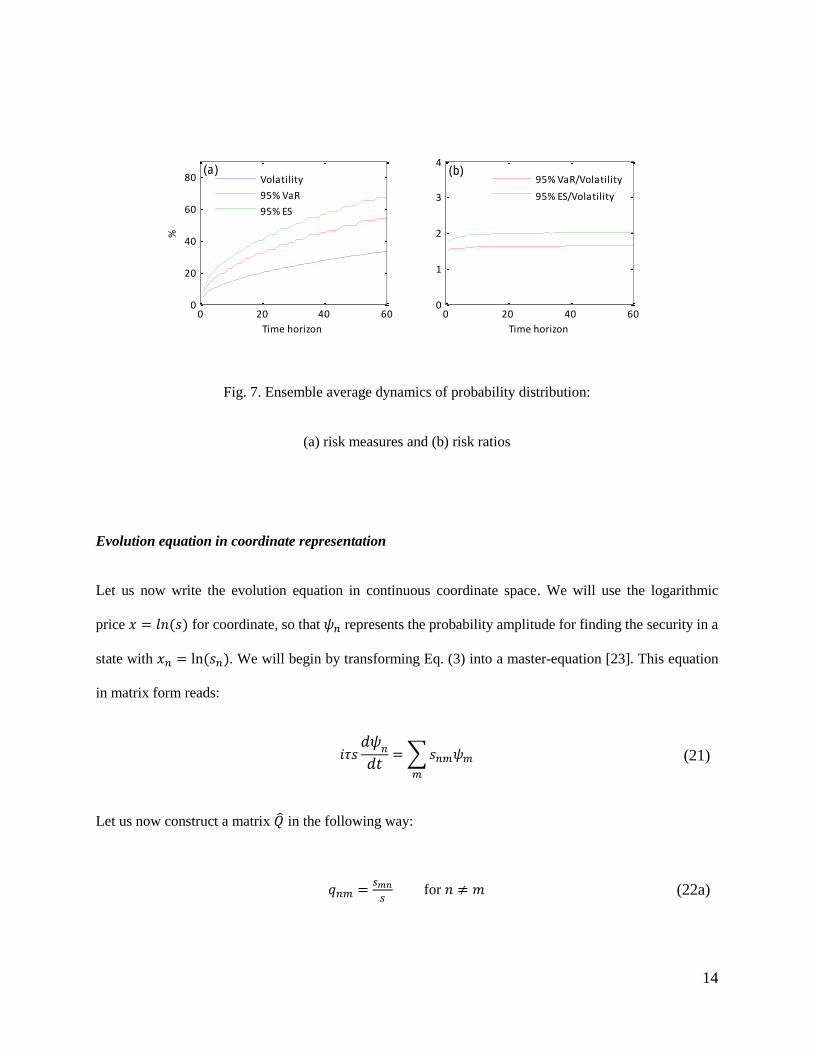
shown in Fig. 5c, exhibit a √𝑡-like behavior. They are also erratic and can deviate from Gaussian values,
which is evidenced by risk ratios on Fig. 5d (1.64 for 95% VaR and 2.06 for 95% Expected Shortfall). This
deviation is especially large at smaller time scale and diminishes with time. Ensemble average produces
smooth curves, shown in Figs. 6,7. Even though an ensemble allows to take into account all possibilities,
in reality we must face only a single realization, with its erratic behavior.
Fig. 4. Dynamics of probability distribution in a single realization
time
x (%
)
10 20 30 40 50 60
-100
-50
0
50
0
0.1
0.2
0.3
0.4
0.5

13
Fig. 5. Dynamics of probability distribution in single realization: (a) initial and final probability
distributions, (b) dynamics of probabilities, (c) risk measures, and (d) risk ratios
Fig. 6. Ensemble average dynamics of probability distribution.
-100 -50 0 50 1000
0.1
0.2
0.3
0.4
x, (%)
Pro
bab
ilit
y
(a)
Initial
Final
0 20 40 600
0.1
0.2
0.3
0.4
Time horizon
Pro
bab
ilit
y
(b)
return = 0%
return = -10%
return = -20%
0 20 40 600
20
40
60
80
Time horizon
%
(c)
Volatility
95% VaR
95% ES
0 20 40 600
1
2
3
4
Time horizon
(d)
95% VaR/Volatility
95% ES/Volatility
time
x (%
)
10 20 30 40 50 60
-100
-50
0
500.05
0.1
0.15
0.2
14
Fig. 7. Ensemble average dynamics of probability distribution:
(a) risk measures and (b) risk ratios
Evolution equation in coordinate representation
Let us now write the evolution equation in continuous coordinate space. We will use the logarithmic
price 𝑥 = 𝑙𝑛(𝑠) for coordinate, so that 𝜓𝑛 represents the probability amplitude for finding the security in a
state with 𝑥𝑛 = ln(𝑠𝑛). We will begin by transforming Eq. (3) into a master-equation [23]. This equation
in matrix form reads:
𝑖𝜏𝑠
𝑑𝜓𝑛
𝑑𝑡= ∑𝑠𝑛𝑚𝜓𝑚
𝑚
(21)
Let us now construct a matrix �̂� in the following way:
𝑞𝑛𝑚 =
𝑠𝑚𝑛
𝑠 for 𝑛 ≠ 𝑚 (22a)
-100 -50 0 50 1000
0.1
0.2
x, (%)
Pro
bab
ilit
y
(a)
Initial
Final
Avg. final
0 20 40 600
0.1
0.2
Time horizon
Pro
bab
ilit
y
(b)
return = 0%
return = -10%
return = -20%
0 20 40 600
20
40
60
80
Time horizon
%(a)
Volatility
95% VaR
95% ES
0 20 40 600
1
2
3
4
Time horizon
(b)
95% VaR/Volatility
95% ES/Volatility

15
𝑞𝑛𝑛 =∑ 𝑠𝑙𝑛𝑙
𝑠 (22b)
Then matrix elements of �̂� and �̂� are connected through the following relation:
𝑠𝑛𝑚 = 𝑠 (𝑞𝑚𝑛 − 𝛿𝑛𝑚 ∑𝑞𝑛𝑙
𝑙≠𝑛
) (23)
where 𝑠 is factored out so that matrix coefficients do not scale with price. Eq. (21) now transforms into:
𝑖𝜏
𝑑𝜓𝑛
𝑑𝑡= ∑𝑞𝑚𝑛𝜓𝑚
𝑚
− ∑ 𝑞𝑛𝑚𝜓𝑛
𝑚≠𝑛
(24)
This equation has a form of a master-equation. In nearest-neighbor approximation we have:
𝑖𝜏
𝑑𝑓𝑛
𝑑𝑡= 𝑞𝑛−1,𝑛𝑓𝑛−1 − (𝑞𝑛,𝑛−1 + 𝑞𝑛,𝑛+1)𝑓𝑛 + 𝑞𝑛+1,𝑛𝑓𝑛+1 (25)
where we used the 𝜓𝑛 = 𝑒−𝑖𝑞𝑛𝑛𝑡
𝜏𝑓𝑛 substitution. Let us introduce the functions 𝜇 and 𝛾, such that
𝑖𝜇𝑛 = Δ𝑥(𝑞𝑛,𝑛−1 − 𝑞𝑛,𝑛+1) (26a)
𝛾𝑛 =
Δ𝑥2
2(𝑞𝑛,𝑛−1 + 𝑞𝑛,𝑛+1) (26b)
Elements 𝑞𝑛𝑚 can be expressed through these functions as
𝑞𝑛𝑚 = 𝜅𝑛𝛿𝑛−1,𝑚 + 𝜅𝑚∗ 𝛿𝑛+1,𝑚 (27a)
𝜅𝑛 =𝛾𝑛
Δ𝑥2+ 𝑖
𝜇𝑛
2Δ𝑥 (27b)
Performing transition to continuous form we arrive at the following Fokker-Planck equation:

16
𝑖𝜏
𝜕𝑓
𝜕𝑡= 𝑖
𝜕(𝜇𝑓)
𝜕𝑥+
𝜕2(𝛾𝑓)
𝜕𝑥2 (28)
Here 𝜇 = 𝜇(𝑥, 𝑡) and 𝛾 = 𝛾(𝑥, 𝑡) are generally functions of coordinate and time. If 𝜇 and 𝛾 fluctuate in
time, then an ensemble average should be taken according to Eq. (16) in order to obtain a complete
probability distribution. The 𝜕
𝜕𝑥 term is responsible for the drift of probability amplitude in coordinate space,
and the 𝜕2
𝜕𝑥2 term is responsible for dispersion. We do not make a statement that 𝛾 necessarily has to have a
definite sign, since we are developing a theory without drawing any prior similarities to traditional quantum
mechanics. Properties of 𝜇 and 𝛾 have to be established by further research as it relates to financial markets.
Equation Eq. (28) combined with initial condition 𝑓(𝑥, 𝑡 = 0) = 𝑓0(𝑥) formulates an initial value problem
that describes evolution of probability amplitude of security’s logarithmic price (or effectively returns) with
time.
3. Probability evolution
Let us now apply Eq. (28) to study evolution of price probabilities. We will assume the initial price to be
localized with width 𝑤0 according to Gaussian probability distribution, so the probability amplitude is:
𝑓(𝑥, 0) =
1
√2𝜋𝑤024𝑒
−𝑥2
4𝑤02 (29)
That way ∫ 𝑝(𝑥)𝑑𝑥∝
−∝= ∫ |𝑓(𝑥, 0)|2𝑑𝑥 = 1
∝
−∝. We will model the fluctuating parameters 𝜇(𝑥, 𝑡) and 𝛾(𝑥, 𝑡)
piecewise in time, refreshing them after each time step:
17
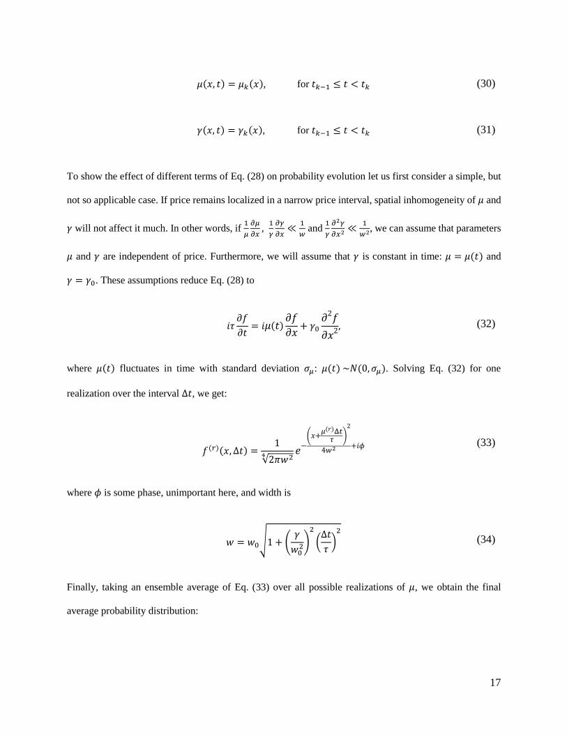
𝜇(𝑥, 𝑡) = 𝜇𝑘(𝑥), for 𝑡𝑘−1 ≤ 𝑡 < 𝑡𝑘 (30)
𝛾(𝑥, 𝑡) = 𝛾𝑘(𝑥), for 𝑡𝑘−1 ≤ 𝑡 < 𝑡𝑘 (31)
To show the effect of different terms of Eq. (28) on probability evolution let us first consider a simple, but
not so applicable case. If price remains localized in a narrow price interval, spatial inhomogeneity of 𝜇 and
𝛾 will not affect it much. In other words, if 1
𝜇
𝜕𝜇
𝜕𝑥,
1
𝛾
𝜕𝛾
𝜕𝑥≪
1
𝑤 and
1
𝛾
𝜕2𝛾
𝜕𝑥2 ≪1
𝑤2, we can assume that parameters
𝜇 and 𝛾 are independent of price. Furthermore, we will assume that 𝛾 is constant in time: 𝜇 = 𝜇(𝑡) and
𝛾 = 𝛾0. These assumptions reduce Eq. (28) to
𝑖𝜏
𝜕𝑓
𝜕𝑡= 𝑖𝜇(𝑡)
𝜕𝑓
𝜕𝑥+ 𝛾0
𝜕2𝑓
𝜕𝑥2, (32)
where 𝜇(𝑡) fluctuates in time with standard deviation 𝜎𝜇: 𝜇(𝑡)~𝑁(0, 𝜎𝜇). Solving Eq. (32) for one
realization over the interval Δ𝑡, we get:
𝑓(𝑟)(𝑥, Δ𝑡) =1
√2𝜋𝑤24 𝑒−
(𝑥+𝜇(𝑟)Δ𝑡
𝜏 )
2
4𝑤2 +𝑖𝜙
(33)
where 𝜙 is some phase, unimportant here, and width is
𝑤 = 𝑤0√1 + (𝛾
𝑤02)
2
(Δ𝑡
𝜏)2
(34)
Finally, taking an ensemble average of Eq. (33) over all possible realizations of 𝜇, we obtain the final
average probability distribution:
18
𝑃(𝑥) = 𝐸𝑟 [|𝑓(𝑟)(𝑥, 𝑡)|
2] =
1
√2𝜋𝑤(𝑡)2𝑒
−𝑥2
2𝑤(𝑡)2 (35)
where width is given by:
𝑤(𝑡) = 𝑤0√1 +𝜎𝜇
2
𝑤02
𝑡
𝜏+ (
𝛾
𝑤02)
2
(𝑡
𝜏)2
(36)
Thus, when inhomogeneity is small probability distribution maintains Gaussian shape during evolution,
both in a single realization and in ensemble average. An example of this can be seen in Figs. 8,9, that show
that risk ratios constantly remain on their Gaussian levels: 1.64 and 2.06.
In this model temporal behavior of the width changes from square root behavior linear, which is not
physical. This is not surprising, since we made assumptions that make the solution valid only for small
timeframe, in which inhomogeneity of trading environment does not come into play. More specifically,
equation Eq. (36) can only be applied at timescale 𝑡 ≲ (𝑤0𝜎𝜇
𝛾)2𝜏.

19
Fig. 8. Dynamics of probability distribution:
(a) single realization (b) ensemble average over 100 realizations
time
x (%
)
(a)
10 20 30 40 50 60
-100
-50
0
50
100 0
0.05
0.1
time
x (%
)
(b)
10 20 30 40 50 60
-100
-50
0
50
100 0
0.05
0.1

20
Fig. 9. Dynamics of probability distribution:
(a) initial, final, and average final probability distributions, (b) dynamics of probabilities, (c) risk
measures, and (d) risk ratios
Probability evolution in random trading environment
While Eq. (28) allows to study numerous models with various types of dependencies of 𝜇 and 𝛾, and having
various log-price structures, let us consider a model with large disorder, leading to complete randomization
of phase at each step of evolution. Let 𝜇 fluctuate in time: 𝜇 = 𝜇(𝑡), and 𝛾 fluctuate in both time and price:
𝛾 = 𝛾(𝑥, 𝑡), and let 𝛾 have granularity size 𝜖 = Δ𝑥 in price, so that values in the neighboring price levels
-100 -50 0 50 1000
0.05
0.1
x, (%)
Pro
bab
ilit
y
(a)
Initial
Final
Avg. final
0 20 40 600
0.05
0.1
Time horizon
Pro
bab
ilit
y
(b)
return = 0%
return = -10%
return = -20%
0 20 40 600
20
40
60
80
Time horizon
%
(c)
Volatility
95% VaR
95% ES
0 20 40 600
1
2
3
4
Time horizon
(d)
95% VaR/Volatility
95% ES/Volatility

21
are uncorrelated. We thus have for Eq. (27b): 𝜇𝑛 = 𝜇~𝑁(0, 𝜎𝜇) and 𝛾𝑛 = 𝑁(0, 𝜎𝛾). Standard deviations 𝜎𝜇
and 𝜎𝛾 must be chosen so that the eigenvalues of the price operator match the 1-step price spectrum.
Evolution of probability amplitude in such environment can be approached by representing it as a
superposition of probability amplitudes at different price levels:
𝜓(𝑥, 𝑡) = ∫ 𝑎𝜌(𝑥′)𝜓𝜖(𝑥
′ − 𝑥, 𝑡)𝑑𝑥′
∞
−∞
(37)
where 𝜓𝜖 is localized within the range 𝜖, and 𝑎𝜌 is an envelope function with width 𝜌, such that relation
𝑤2 = 𝜌2 + 𝜖2 is maintained.
Width of propagated amplitude 𝜓𝜖(𝑥, 𝑡 + Δ𝑡) is described by Eq. (36) and grows if 𝜏 decreases. However,
the maximum value it can take in a single step is ~3𝜖, because only the neighboring levels interact. At
small enough 𝜏, such that 𝜏 ≳𝛾Δ𝑡
𝜋𝑤2 the level of disorder is so high that phase begins to change randomly
with price and its values cover the entire interval (−𝜋; 𝜋]. At this point we can neglect interference and
present the propagated distribution as:
|𝜓(𝑥, 𝑡 + Δ𝑡)|2 = ∫ 𝑎𝜌
2(𝑥′)|𝜓𝜖(𝑥′ − 𝑥, 𝑡 + Δ𝑡)|2𝑑𝑥′
∞
−∞
(38)
As a result, the probability distribution only widens randomly by about one level in each evolution step:
𝑤2(𝑡 + Δ𝑡) = 𝑤2(𝑡) + (𝛽𝜖)2 (39)
where 𝛽~1. Thus, when 𝜏 becomes too small width 𝑤 levels off and ceases its direct dependence on 𝜎𝜇 and
𝜎𝛾. No matter how much further 𝜏 is decreased, it will no effect on dynamics of 𝜓. We can see that effect
in Fig. 10, presenting the 𝑤(𝑇) as it changes with 1
𝜏.

22
Fig. 10. Saturation of final width 𝑤(𝑇) with 1
𝜏.
Another way to see this is by analyzing the propagation operator
�̂� = 𝑒−𝑖�̂�
Δ𝑡𝜏 (40)
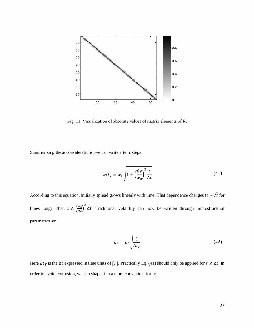
Since �̂� is a tridiagonal matrix, �̂� is almost tridiagonal, meaning that the only elements substantially
different from zero are the diagonal and its adjacent elements [24,25]. This fact does not change if 𝜏
diminishes. However, diminishing 𝜏 randomizes the phases at the adjacent nodes. Visualization of absolute
values of �̂� is provided in Fig. 11. We can say that 𝑅(𝑥, 𝑥′) are random and have standard deviation ~𝜖 in
dimension 𝑥′. As a result, variance of the resulting distribution |𝜓(𝑥, Δ𝑡)|2 widens by about 𝜖 after each
step of propagation, which brings us back to Eq. (39).
0 50 100 150 200 250 3000
5
10
15
20
25
30
35
40
45
50
1/
Fin
al w
idth
, %
23
Fig. 11. Visualization of absolute values of matrix elements of �̂�.
Summarizing these considerations, we can write after 𝑡 steps:
𝑤(𝑡) = 𝑤0√1 + (𝛽𝜖
𝑤0)2 𝑡
Δ𝑡 (41)
According to this equation, initially spread grows linearly with time. That dependence changes to ~√𝑡 for
times longer than 𝑡 ≳ (𝑤0
𝛽𝜖)2Δ𝑡. Traditional volatility can now be written through microstructural
parameters as:
𝜎𝑇 = 𝛽𝜖√
1
Δ𝑡𝑇 (42)
Here Δ𝑡𝑇 is the Δ𝑡 expressed in time units of [𝑇]. Practically Eq. (41) should only be applied for 𝑡 ≥ Δ𝑡. In
order to avoid confusion, we can shape it in a more convenient form:
20 40 60 80
10
20
30
40
50
60
70
80
0
0.2
0.4
0.6
0.8

24
𝑤(𝑡) = 𝑤Δ𝑡 √1 + (𝛽𝜖
𝑤Δ𝑡)2
(𝑡
Δ𝑡− 1) (43)
where
𝑤Δ𝑡 = 𝑤0√1 + (𝛽𝜖
𝑤0)2
(44)
Behavior of 𝑤(𝑡) repeats the conclusions of [2]. We see that the randomness of trading environment
combined with the local character of interaction between price levels leads to diffusion of probability
amplitude in price space. Localization width given by Eq. (43) allows to blend the intrinsic bid-ask spread
at small time scale with the √𝑡 diffusion-like behavior at large time scale.
4. Calibration to market data
In this section we demonstrate how this model works in practice. We will consider the high-low bar data as
spread4 and set the initial probability width equal to average 1-step spread. We then calibrate 𝜎𝜇 and 𝜎𝛾 to
fit the 1-step price spectrum. Next, we choose 𝜏 at which the spread curve 𝑤(𝑇) stabilizes. With these
parameters we generate probability amplitude dynamics in a number of realizations.
Risk values (VaR and Expected Shortfall) are computed as averages over the ensemble, and not as measures
of the average distribution:
𝑅𝑖𝑠𝑘 = ⟨𝑅𝑖𝑠𝑘(𝑟)⟩𝑟 (45)
4 Possibility of a more general interpretation of spread than just plain bid-ask spread was mentioned earlier.

25
Calibration to intraday 1-minute high-low data for LULU
Figs. 12-14 present calibrated plots for minute-scale high-low bar data for Lululemon Athletica Inc. (ticker
LULU) on March 16, 2016. LULU is an average liquidity NASDAQ-listed stock and on that date its 1.2
mln. shares traded with average relative bid-ask spread 0.06% and average trading time 3.2 sec.
Fig. 12a-b show a single scenario and an ensemble average of probability distribution dynamics. Fig. 13a
allows to compare the initial and final probability distributions, whereas the final distributions are shown
as a single scenario and ensemble average. Time evolution of probabilities of various returns is shown in
Figs. 13b. Risk measures – volatility, 95% VaR, and 95% Expected shortfall – are shown in Figs. 13c.
Finally, the relation of risk measures to their Gaussian benchmarks are shown in Figs. 13d. Spread curve
can also be obtained directly from Eq. (43) with 𝑤Δ𝑡 = 0.07% and 𝛽𝜖 =0.001 and is shown in Fig. 14.
We continue providing calibrated data for probability distribution of daily high-lows of LULU in
Figs. 15-17. Lastly, Figs. 18-23 show calibrated data for probability distributions of 1-minute and daily
high-lows for APPL.

26
Fig. 12. Dynamics of probability distribution of intraday 1-minute high-lows for LULU ticker:
(a) single realization (b) ensemble average over 100 realizations
time (minutes)
x (%
)
(a)
10 20 30 40 50 60
-3
-2
-1
0
1
20.05
0.1
0.15
0.2
0.25
0.3
0.35
time (minutes)
x (%
)
(b)
10 20 30 40 50 60
-3
-2
-1
0
1
20.05
0.1
0.15
0.2
0.25
0.3
0.35

27
Fig. 13. Dynamics of probability distribution of intraday 1-minute high-lows for LULU ticker:
(a) initial, final, and average final probability distributions, (b) dynamics of probabilities, (c) risk
measures, and (d) risk ratios
-4 -2 0 2 40
0.1
0.2
0.3
0.4
x, (%)
Pro
bab
ilit
y
(a)
Initial
Final
Avg. final
0 20 40 600
0.2
0.4
0.6
0.8
1
Time horizon (minutes)
Pro
bab
ilit
y
(b)
return = 0%
return = -0.5%
return = -1%
0 20 40 600
0.5
1
1.5
2
Time horizon (minutes)
%
(c)
Volatility
95% VaR
95% ES
0 20 40 600
1
2
3
4
Time horizon (minutes)
(d)
95% VaR/Volatility
95% ES/Volatility

28
Fig. 14. Spread curve of LULU on March 16, 2016 and its fit with Eq. (43) using 𝑤Δ𝑡 = 0.07%
and 𝛽𝜖 =0.001. The average bid-ask spread was also equal 0.06%.
Calibration to daily high-low data for LULU
Fig. 15. Dynamics of probability distribution of daily high-lows for LULU ticker:
(a) single realization (b) ensemble average over 100 realizations
0.0%
0.2%
0.4%
0.6%
0.8%
1.0%
- 20 40 60
Time (min)
High-low
w(T)
time (days)
x (%
)
(a)
10 20 30 40 50 60
-100
0
100
time (days)
x (%
)
(b)
10 20 30 40 50 60
-100
0
100
0
0.05
0.1
0.15
0.2
0.25
0
0.05
0.1
0.15
0.2
0.25

29
Fig. 16. Dynamics of probability distribution of daily high-lows for LULU ticker:
(a) initial, final, and average final probability distributions, (b) dynamics of probabilities, (c) risk
measures, and (d) risk ratios
-200 -100 0 100 2000
0.1
0.2
0.3
0.4
x, (%)
Pro
bab
ilit
y
(a)
Initial
Final
Avg. final
0 20 40 600
0.1
0.2
0.3
0.4
Time horizon (days)
Pro
bab
ilit
y
(b)
return = 0%
return = -10%
return = -20%
0 20 40 600
20
40
60
80
Time horizon (days)
%
(c)
Volatility
95% VaR
95% ES
0 20 40 600
1
2
3
4
Time horizon (days)
(d)
95% VaR/Volatility
95% ES/Volatility

30
Fig. 17. Spread curve of LULU, based on daily high-low data, and its fit with Eq. (43) using
𝑤Δ𝑡 = 3.17% and 𝛽𝜖 =0.0379. Difference is barely discernable.
Calibration to intraday 1-minute high-low data for AAPL
Fig. 18. Dynamics of probability distribution of intraday 1-minute high-lows for AAPL ticker:
(a) single realization (b) ensemble average over 100 realizations
0%
5%
10%
15%
20%
25%
30%
35%
- 20 40 60
Time (days)
High-low
w(T)
time (minutes)
x (%
)
(a)
10 20 30 40 50 60
-2
-1
0
1
0
0.05
0.1
0.15
0.2
0.25
time (minutes)
x (%
)
(b)
10 20 30 40 50 60
-2
-1
0
1
0
0.05
0.1
31
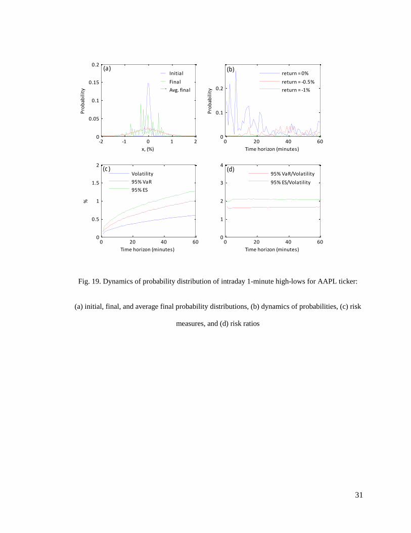
Fig. 19. Dynamics of probability distribution of intraday 1-minute high-lows for AAPL ticker:
(a) initial, final, and average final probability distributions, (b) dynamics of probabilities, (c) risk
measures, and (d) risk ratios
-2 -1 0 1 20
0.05
0.1
0.15
0.2
x, (%)
Pro
bab
ilit
y
(a)
Initial
Final
Avg. final
0 20 40 600
0.1
0.2
Time horizon (minutes)
Pro
bab
ilit
y
(b)
return = 0%
return = -0.5%
return = -1%
0 20 40 600
0.5
1
1.5
2
Time horizon (minutes)
%
(c)
Volatility
95% VaR
95% ES
0 20 40 600
1
2
3
4
Time horizon (minutes)
(d)
95% VaR/Volatility
95% ES/Volatility

32
Fig. 20. Spread curve of AAPL on March 16, 2016 and its fit with Eq. (43) using 𝑤Δ𝑡 = 0.07%
and 𝛽𝜖 =0.00072. The average bid-ask spread was 0.01%, which corresponds to spread of $0.01.
Calibration to daily high-low data for AAPL
Fig. 21. Dynamics of probability distribution of daily high-lows for AAPL ticker:
(a) single realization (b) ensemble average over 50 realizations
0.0%
0.1%
0.2%
0.3%
0.4%
0.5%
0.6%
- 20 40 60
Time (min)
High-low
w(T)
time (days)
x (%
)
(a)
10 20 30 40 50 60
-50
0
50
0.05
0.1
0.15
0.2
time (days)
x (%
)
(b)
10 20 30 40 50 60
-50
0
50
0.02
0.04
0.06
0.08

33
Fig. 22. Dynamics of probability distribution of daily high-lows for AAPL ticker:
(a) initial, final, and average final probability distributions, (b) dynamics of probabilities, (c) risk
measures, and (d) risk ratios
-50 0 500
0.02
0.04
0.06
0.08
0.1
x, (%)
Pro
bab
ilit
y
(a)
Initial
Final
Avg. final
0 20 40 600
0.02
0.04
0.06
0.08
0.1
Time horizon (days)
Pro
bab
ilit
y
(b)
return = 0%
return = -10%
return = -20%
0 20 40 600
20
40
60
80
Time horizon (days)
%
(c)
Volatility
95% VaR
95% ES
0 20 40 600
1
2
3
4
Time horizon (days)
(d)
95% VaR/Volatility
95% ES/Volatility

34
Fig. 23. Spread curve of AAPL, based on daily high-low data, and its fit with Eq. (43) using
𝑤Δ𝑡 = 1.97% and 𝛽𝜖 =0.0241.
5. Discussion and conclusions
Thus, we showed that price forms as a result of selection out of the entire spectrum of prices according to
probability of the security to be in each corresponding state. Price spectrum is represented by a price
operator whose matrix elements fluctuate in time. In matrix form dynamics of probability distribution obeys
the Schrodinger equation with properly build price operator. In log-price coordinate representation
probability distribution obeys the Fokker-Planck equation with complex coefficients. Price remains
localized within a range until the act of measurement, which occurs at the time of transaction.
As a result of this framework we showed that return probability distribution, usually thought to be a smooth
bell shaped curve, is not actually bell shaped at all. Even though localized in price, it is erratic, and its
evolution is also erratic! Only after averaging over many possible scenarios it becomes smooth. However,
in reality we must face a single scenario with its erratic behavior, not an ensemble average. This in turn
means that any price shift, even big, can at times build up a good chance of occurring and lead to the so
called “Black Swans”.
0%
5%
10%
15%
20%
- 20 40 60
Time (days)
High-low
w(T)

35
Although probability behavior is erratic the distribution width grows slowly, exhibits strong non-Gaussian
features at small time scale, and the √𝑡 behavior at large time scale. This diffusion-like behavior has its
origin in randomness of phase noise introduced by the fluctuations of trading environment and the close
range of price level interaction.
Despite the apparent similarity between Schrodinger and diffusion equations, one cannot be thought of as
a direct extension of the other only with an imaginary diffusion coefficient5. Physical solutions of the two
are completely different: Schrodinger equation provides solutions that are oscillatory and diffusion equation
provides solutions that are dissipative. Yet, disorder of environment can alter the time dependence of the
probability distribution’s width and even lead to complete loss of it [26].
Up to date using quantum framework of price formation we have been able to describe the following
elements of financial markets:
1) statistical behavior of spread and mid-price [1]
2) spread’s scaling behavior [1,2]
3) spread curve blending the minimum spread with the √𝑡 power law [present work]
4) relationship between spread, volatility and volume [2]
5) fat tails and rare events [present work]
Along with this progress there are difficulties as well, at least that’s how they currently look. One of them
is the linearity of the theory’s basic equations. Linearity of equations implies validity of the superposition
principle and eliminates chances of direct self-action. There is no clear evidence that this can be said of
financial markets. Doubling an order size does not necessarily lead to a doubling effect on price localization.
Even worse, it can start processes that were impossible with a lower order size.
5 Even though analytic continuation is possible under certain constraints.

36
Another difficulty lies in responsive nature of financial markets. As a comparison, in measuring physical
properties of elementary particles, the measuring device does not affect the quantity under measurement
until it comes in contact with the object. Financial markets are different. Even in the absence of transactions
traders on buy and sell sides affect each other’s actions. As a result of that security price may be affected
before it is measured.
An element that was seemingly left out of the theory is the order size. Order size affects price and is one of
the main characteristics of a transaction. Some light has been shed on the issue in our work [2], where
relationship between order size, transaction frequency, spread and volatility is studied.
It is also not obvious how quantum approach can describe situations with limited free float, or equities of
companies under the acquisition process, where equity price is primarily dictated by the acquirer. We tend
to think that answers to these questions will come as a result of further research.
Summarizing, we have expanded the basic framework proposed by us in [1] and developed a price
formation theory based on the nature of price and price measurement process. This framework deals with
spread as its intrinsic property and provides a smooth transition from small time scale when spread is
important to large time scale when spread becomes unimportant.
This theory opens new capabilities for financial institutions that are involved in market-making and
securities dealing activities. It allows to model price evolution in a consistent way and we have shown that
behavior resulting from this framework agrees with measurable market data. This model can be calibrated
to various types of data, such as best bid-and-ask, effective bid-ask, or even OHLC bars. Using the
calibrated model firms and trading desks can price securities, particularly ones with limited liquidity,
measure risk associated with spread, gauge it against the regular mid-price risk, and protect against rare
undesired events. All these capabilities are extremely important when a trading desk’s risk/return profile
substantially depends on spread.

37
6. References
[1] J. Sarkissian, “Coupled mode theory of stock price formation”, arXiv:1312.4622v1 [q-fin.TR], (2013)
[2] J. Sarkissian, “Volume, Spread, and Volatility Relation in Financial Markets and Market Maker’s Profit
Optimization”, to be published
[3] A.B. Schmidt, “Financial Markets and Trading: An Introduction to Market Microstructure and Trading
Strategies”, Wiley; 1 edition (August 9, 2011)
[4] A.P. Nawroth and J. Peinke, “Small scale behavior of financial data”, Physics Letters A, 360, 234,
(2006)
[5] T-W. Yang, L. Zhu, “A reduced-form model for level-1 limit order books”, arXiv:1508.07891v3 [q-
fin.TR], http://arxiv.org/abs/1508.07891, (2015)
[6] I.M. Toke, N. Yoshida, “Modelling intensities of order flows in a limit order book”, arXiv:1602.03944
[q-fin.ST], http://arxiv.org/abs/1602.03944, (2016)
[7] M. Avellaneda, S. Stoikov, “High-frequency trading in a limit order book”, Quantitative Finance 8(3),
217–224 (2008)
[8] O. Gueant, C.-A. Lehalle, and J. Fernandez-Tapia, “Dealing with the inventory risk: a solution to the
market making problem", Mathematics and Financial Economics, Volume 7, Issue 4, pp 477-507, (2013)
[9] P. A. M. Dirac, “The Principles of Quantum Mechanics”, (Oxford Univ Pr., 1982)
[10] M. Schaden, “Quantum finance”, Physica A 316 (2002) 511-538.
[11] M. Schaden, “A quantum approach to stock price fluctuations”, arXiv:physics/0205053v2, (2003)

38
[12] C. Zhang, L. Huang, “A quantum model for the stock market”, arXiv:1009.4843v2 [q-fin.ST], (2010)
[13] O. Choustova, “Toward Quantum-like Modelling of Financial Processes”, arXiv:quant-ph/0109122v5,
(2007)
[14] C.P. Gonçalves, “Financial Market Modeling with Quantum Neural Networks”, arXiv:1508.06586
(2015)
[15] Z. Chen (2004). "Quantum Theory for the Binomial Model in Finance Theory". Journal of Systems
Science and Complexity. arXiv:quant-ph/0112156. Bibcode:2001quant.ph.12156C.
[16] X. Meng, J-W. Zhang, H. Guoa, “Quantum Brownian motion model for the stock market”, Physica A,
Volume 452, 15 June 2016, Pages 281–288
[17] X. Meng, J-W. Zhang, J. Xu, H. Guo, “Quantum spatial-periodic harmonic model for daily price-
limited stock markets”, Physica A: Statistical Mechanics and its Applications, Volume 438, p. 154-160.
[18] V.A. Nastasiuk, “Emergent quantum mechanics of finances”, Physica A: Statistical Mechanics and its
Applications 403, 148-154
[19] V.A. Nastasiuk, “Fisher information and quantum potential well model for finance”, Physics Letters
A 379 (36), 1998-2000
[20] H-J. Stöckmann, “Quantum Chaos: An Introduction”, Cambridge University Press; 1 edition (March
5, 2007)
[21] L.D. Landau, E.M. Lifshitz, “Quantum Mechanics: Non-Relativistic Theory”. Vol. 3, 3rd ed.,
(Butterworth-Heinemann, 1981)
[22] B.Ya. Zel’dovich, V.V. Shkunov, T.V. Yakovleva, “Holograms of speckle fields”, Physics Uspekhi,
29, 678-702, (1986)
39
[23] H.J. Carmichael, “Statistical Methods in Quantum Optics 1: Master Equations and Fokker-Planck
Equations (Theoretical and Mathematical Physics) (v. 1)”, Springer (April 25, 2003)
[24] I. Popescu, “General Tridiagonal Random Matrix Models, Limiting Distributions and Fluctuations”,
Probability Theory and Related Fields, May 2009, Volume 144, Issue 1, pp 179-220
[25] Marchenko,V. A., Pastur, L. A. (1967), “Distribution of eigenvalues for some sets of random
matrices”, Mat. Sb. (N.S.), 72(114):4, 507–536
[26] P.W. Anderson, (1958). "Absence of Diffusion in Certain Random Lattices". Phys. Rev. 109 (5): 1492–
1505.