quantummolecularcollisiontheorywithproblemsbasedon matlab ·...
TRANSCRIPT
1
Quantum Molecular Collision Theory with Problems based on
Matlab
Millard H. Alexander
CONTENTS
I. Introduction 2
II. One-dimensional scattering by a barrier 2
A. Rectangular Barrier 2
B. General Potential: Time-independent treatment 6
III. Elastic scattering in three dimensions: Classical treatment 9
A. Separation of center-of-mass motion 9
B. Scattering in the center-of-mass frame 9
C. Classical differential cross section 16
IV. Elastic scattering in three dimensions: quantum treatment 20
A. Separation of radial and angular motion 20
B. Numerical determination of the scattering wavefunction 22
C. Phase shift 26
D. Scattering boundary conditions 32
E. Determination of f(θ) 33
F. Integral Cross Section 36
V. Inelastic Scattering 37
A. Generalities 37
B. The renormalized Numerov method in the asymptotic basis 39
C. Determination of the log-derivative matrix 42
D. Operational outline of the renormalized Numerov method 44
E. Determination of the S matrix 45
F. Illustrative calculation: Asymptotic basis 47

2
G. Using the renormalized Numerov method in the locally adiabatic basis 49
H. Determination of the log-derivative matrix in the asymptotic basis 53
I. Initialization and propagation algorithm: locally-adiabatic basis 54
J. Illustrative calculation 56
K. Enhanced Numerov propagator 56
L. Advantages of the locally-adiabatic propagation 57
VI. Rotationally Inelastic Scattering 58
A. Partial Wave Decomposition 59
VII. Collinear Reactive Scattering 59
A. Bond, Jacobi, and mass-scaled Jacobi coordinates 59
B. Relation between arrangement Jacobi coordinates 63
VIII. Finite Element Solution of the Schroedinger equation 65
A. Generalities 65
B. Boundary integral 68
IX. Evaluation of the matrices 71
References 72
I. INTRODUCTION
In these lectures, I will present an Introduction to some key concepts and ideas in the
quantum description of molecular collisions. Working through these topics, and the associ-
ated problems, will give you the background to embark on a research career in theoretical
chemistry
II. ONE-DIMENSIONAL SCATTERING BY A BARRIER
A. Rectangular Barrier
Consider one-dimensional scattering by a rectangular barrier, illustrated here

3
x
V(x)
0 a
V0
I II III
FIG. 1. A one-dimensional rectangular barrier of height V0 and width a.
Since the potential is constant (and equal to zero) in region I, the wavefunction, which
is a solution to the one-dimensional, time-independent Schrodinger equation
Hψ = [KEop + V (x)] =
[
− h2
2m
d2
dx2+ V (x)
]
ψ = Eψ
can be written as
ψI = eikx +Re−ikx (1)
where the wavevector is defined as k = (2mE/h2)1/2. This corresponds to an incoming
wave propagating to the right and a reflected wave, with amplitude R. In region III the
wavefunction can be written as
ψIII = Seikx (2)
which corresponds to a scattered wave with amplitude S. Obviously |S|2 + |R|2 = 1, since
flux has to be conserved. In region II, the form of the wavefunction depends on whether
the energy is greater than or less than V0. In the former case, which corresponds to the
classically allowed situation, we have
ψII = Aeik′x +Be−ik′x (3)
where k′ = [2m(E − V0)/h2]1/2. When E < V0, the form of the wavefunction is
ψII = Aeκx +Be−κx (4)
4
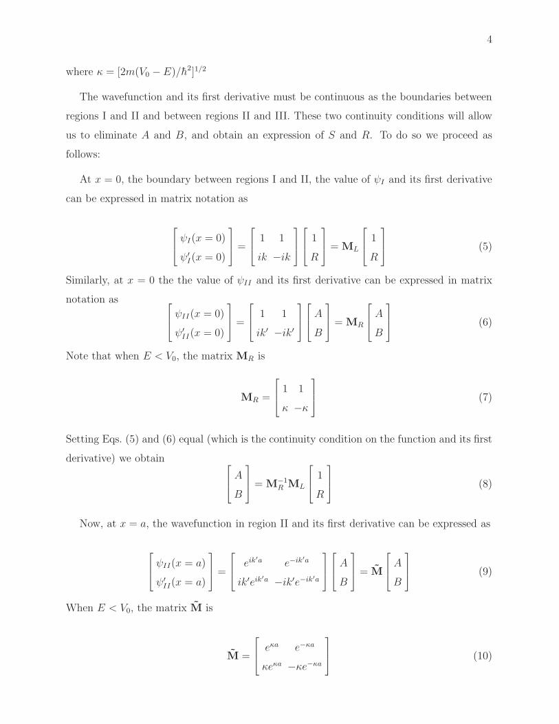
where κ = [2m(V0 −E)/h2]1/2
The wavefunction and its first derivative must be continuous as the boundaries between
regions I and II and between regions II and III. These two continuity conditions will allow
us to eliminate A and B, and obtain an expression of S and R. To do so we proceed as
follows:
At x = 0, the boundary between regions I and II, the value of ψI and its first derivative
can be expressed in matrix notation as
ψI(x = 0)
ψ′I(x = 0)
=
1 1
ik −ik
1
R
= ML
1
R
(5)
Similarly, at x = 0 the the value of ψII and its first derivative can be expressed in matrix
notation as
ψII(x = 0)
ψ′II(x = 0)
=
1 1
ik′ −ik′
A
B
= MR
A
B
(6)
Note that when E < V0, the matrix MR is
MR =
1 1
κ −κ
(7)
Setting Eqs. (5) and (6) equal (which is the continuity condition on the function and its first
derivative) we obtain
A
B
= M−1R ML
1
R
(8)
Now, at x = a, the wavefunction in region II and its first derivative can be expressed as
ψII(x = a)
ψ′II(x = a)
=
eik′a e−ik′a
ik′eik′a −ik′e−ik′a
A
B
= M
A
B
(9)
When E < V0, the matrix M is
M =
eκa e−κa
κeκa −κe−κa
(10)
5
Also, at x = a the wavefunction in region III and its first derivative can be written as
ψIII(x = a)
ψ′III(x = a)
= S
eika
ikeika
(11)
Now, inserting Eq. (8) into Eq. (9) and equating Eqs. (9) and (10) (the continuity con-
dition at x = a) gives
Seika
ikSeika
= MM−1R ML
1
R
= M
1
R
(12)
Equation (12) is equivalent to solving the following set of linear equations for S and R,
namely
−eika M12
−ikeika M22
S
R
=
−M11
−M21
(13)
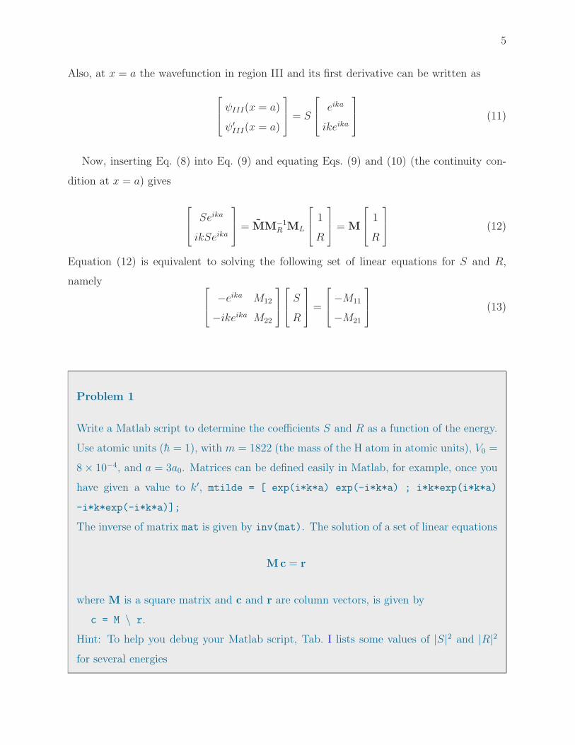
Problem 1
Write a Matlab script to determine the coefficients S and R as a function of the energy.
Use atomic units (h = 1), with m = 1822 (the mass of the H atom in atomic units), V0 =
8× 10⁻⁴, and a = 3a0. Matrices can be defined easily in Matlab, for example, once you
have given a value to k′, mtilde = [ exp(i*k*a) exp(-i*k*a) ; i*k*exp(i*k*a)
-i*k*exp(-i*k*a)];
The inverse of matrix mat is given by inv(mat). The solution of a set of linear equations
Mc = r
where M is a square matrix and c and r are column vectors, is given by
c = M \ r.
Hint: To help you debug your Matlab script, Tab. I lists some values of |S|2 and |R|2
for several energies

6
TABLE I. Square of the scattering and reflection coefficients for scattering by a rectangular barrier.
V0 = 8 × 10⁻⁴, a = 3, m = 1822.
E |R|2 |S|24.10e–4 9.9688e–1 3.1240e–3
8.10e–4 8.5295e–1 1.4705e–1
1.21e–3 7.5028e–2 9.2497e–1
1.61e–3 9.1131e–2 9.0887e–1
2.01e–3 1.7417e–5 9.9998e–1
Problem 2
A plot of the correct values should show that |R|2 goes nearly to zero at the energies
3.0094e-4, 1.2038e-3, and 2.7085e-3. In other words, at these energies there is no reflec-
tion. The collision of the incoming wave proceeds as if there is no barrier at all. Why is
this?
Problem 3
Finally, for a large mass (m=50*1822), at very low energy (e=1×10⁻⁵ hartree), the
square of the scattering amplitude |S|2 becomes larger than one. This is physically
impossible. Why does this result occur?
B. General Potential: Time-independent treatment
Suppose we have an arbitrary potential V (x) which goes to zero as x→ ±∞. At x = −∞,
we designate the two linearly independent solution of the Schrodinger equation as
limx→−∞
ψ(+)(x) = eikx (14)
and
limx→−∞
ψ(−)(x) = e−ikx (15)
7
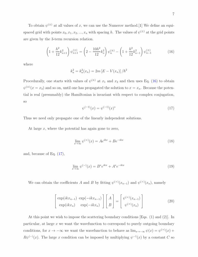
To obtain ψ(±) at all values of x, we can use the Numerov method.[1] We define an equi-
spaced grid with points x0, x1, x2, ..., xn with spacing h. The values of ψ(±) at the grid points
are given by the 3-term recursion relation.
(
1 +h2
12k2n+1
)
ψ(±)n+1 =
(
2− 10h2
12k2n
)
ψ(±)n −
(
1 +h2
12k2n−1
)
ψ(±)n−1 (16)
where
k2n = k2n(xn) = 2m [E − V (xn)] /h2
Procedurally, one starts with values of ψ(±) at x1 and x2 and then uses Eq. (16) to obtain
ψ(±)(x = x3) and so on, until one has propagated the solution to x = xn. Because the poten-
tial is real (presumably) the Hamiltonian is invariant with respect to complex conjugation,
so
ψ(−1)(x) = ψ(−1)(x)∗ (17)
Thus we need only propagate one of the linearly independent solutions.
At large x, where the potential has again gone to zero,
limx→∞
ψ(+)(x) = Aeikx +Be−ikx (18)
and, because of Eq. (17),
limx→∞
ψ(−)(x) = B∗eikx + A∗e−ikx (19)
We can obtain the coefficients A and B by fitting ψ(+)(xn−1) and ψ(+)(xn), namely
exp(ikxn−1) exp(−ikxn−1)
exp(ikxn) exp(−ikxn)
A
B
=
ψ(+)(xn−1)
ψ(+)(xn)
(20)
At this point we wish to impose the scattering boundary conditions [Eqs. (1) and (2)]. In
particular, at large x we want the wavefunction to correspond to purely outgoing boundary
conditions, for x→ −∞ we want the wavefunction to behave as limx→−∞ ψ(x) = ψ(+)(x) +
Rψ(−)(x). The large x condition can be imposed by multiplying ψ−1(x) by a constant C so

8
that
limx→∞
[
ψ(+)(x) + Cψ(−)(x)]
= Seikx
From Eqs. (18) and (19) we see that this can be achieved if
C = −B/A∗
so that
limx→∞
[
ψ(+)(x) + Cψ(−)(x)]
=(
A− BB∗
A∗
)
eikx
Thus,
S = A− |B2|A∗
Similarly, we can use Eqs. (14) and (15) to show that
limx→−∞
[
ψ(+)(x) + Cψ(−)(x)]
= eikx + Ce−ikx = eikx − B
A∗ e−ikx
Thus, the reflection amplitude is
R = − B
A∗ .
Problem 4
Plot the dependence on x of the Eckhart barrier (which is a model for chemical reaction
dynamics), namely
V (x) = V0 sech(ax)2
with V0 = 3× 10⁻⁴, a = 3a0 and where
sech(ax) =1
cosh(ax)=
2
eax + e−ax

9
Problem 5
Modify your Matlab script from subsection A to obtain the scattering and reflection
amplitude for scattering by an Eckhart barrier with m = 1822, V0=8e-4, and a = 3.
Plot the resulting values of |S|2 and |R|2 and compare these with the rectangular barrier
of subsection A. Hint: to check that your script is working, you could propagate to all
x the wavefunctions which have at r → −∞ the asymptotic for given in Eqs. (14) and
(15). These two solutions should be complex conjugates of each other. To make sure
you have the code working properly, Tab. II gives the answers at two energies.
TABLE II. Square of the scattering and reflection coefficients for scattering by an Eckart barrier.
V0 = 8 × 10⁻⁴, a = 1, m = 1822.
E R S |R|2 |S|21.70e–4 –2.9080e–1 + 9.5425e–1 i –6.6528e–2 – 2.0274e–2 i 9.9516e–1 4.8370e–3
1.17e–3 –2.4765e–1 + 2.6432e–2 i –1.0242e–1 – 9.6306e–1 i 6.2030e–2 9.3797e–1
III. ELASTIC SCATTERING IN THREE DIMENSIONS: CLASSICAL
TREATMENT
A. Separation of center-of-mass motion
See the handout I am distributing, taken from the book by McDaniel.[2]
B. Scattering in the center-of-mass frame
Now that we have separated out the motion of the center-of-mass, we need consider only
the scattering of a particle of mass µ by a potential V (r). More details on this classical
treatment can be found in a number of places.[3]
Since the potential depends only on the distance, the angular momentum l is conserved,
namely
l = µr2θ = const (21)
10
where the superscript “dot” indicates differentiation with respect to time. (Note that this
equation is the statement of Kepler’s law – equal angles are swept out in equal time – since
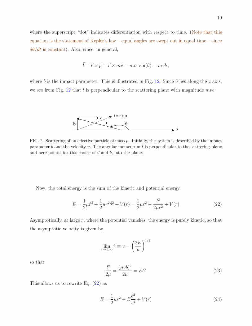
dθ/dt is constant). Also, since, in general,
~l = ~r × ~p = ~r ×m~v = mvr sin(θ) = mvb ,
where b is the impact parameter. This is illustrated in Fig. 12. Since ~v lies along the z axis,
we see from Fig. 12 that l is perpendicular to the scattering plane with magnitude mvb.
Z
v
b
l = r x p
r θ
FIG. 2. Scattering of an effective particle of mass µ. Initially, the system is described by the impact
parameter b and the velocity v. The angular momentum ~l is perpendicular to the scattering plane
and here points, for this choice of ~v and b, into the plane.
Now, the total energy is the sum of the kinetic and potential energy
E =1
2µr2 +
1
2µr2θ2 + V (r) =
1
2µr2 +
l2
2µr2+ V (r) (22)
Asymptotically, at large r, where the potential vanishes, the energy is purely kinetic, so that
the asymptotic velocity is given by
limr→±∞
r ≡ v =
(
2E
µ
)1/2
so thatl2
2µ=
(µvb)2
2µ= Eb2 (23)
This allows us to rewrite Eq. (22) as
E =1
2µr2 + E
b2
r2+ V (r) (24)
11
We can solve this equation for r, obtaining
r = ±
2E
µ
[
1− b2
r2− V (r)
E
]1/2
(25)
Before the collision, at large separation, V (r) is zero so that r = −v = −(2E/µ)1/2. The
particles are approaching so that r is decreasing, thus r is negative. The velocity decreases
until the particles reach their distance of closest approach. At this point r = 0, The value
of r where this occurs defines the turning point, rmin. Mathematically, this is the value of r
for which[
1− b2
r2− V (r)
E
]
= 0
For head-on collisions (zero impact parameter) the turning point occurs where V (r) = E, at
which point all the energy is potential energy. As b increases, the turning point will increase.
Problem 6
Consider the interaction between two argon atoms, which can be well described by a
Morse potential
V (r) = De exp [−2β(r − re)]− 2 exp [−β(r − re)]
with, in atomic units re = 7.1053, β = 0.89305, and De = 4.456× 10⁻⁴.
Write a Matlab function script to determine the value of V (r) for an arbitrary r. Call
this script, say, vmorse(r). Then, write a function script to determine the value of
[
1− b2
r2− V (r)
E
]
.
Call this function, say, term(r), which will be a function only of r. The values of b and E
must also be available to the function script. This can be done by making the variables
b and E “global” (see the Matlab help). This is done by inserting the statement
global E b
in both your calling script (or the command window) and in the function script.
12
Once both vmorse(r) and term(r) are debugged, then you can determine the turning
point by using the Matlab command
rmin=fzero(′term′,xx)
Here xx is an initial numerical guess for the turning point (a good starting point is
xx = 5). Assume that E = 0.006 and use, in an initial check b=0. Check that everything
is working by then calculating the value of
[
1− b2
r2− V (r)
E
]
at the turning point, namely
rmin=fzero(′term′,xx); term(rmin)
You’ll sometimes find (depending on E and b) that fzero will give you a turning
point for which the term in square brackets is negative, so that you’re slightly inside
the true turning point. To correct for this, add a small number to the turning point, in
other words, define the turning point as
rmin=fzero(′term′,xx)+1.e-12
Now, plot the turning point as a function of impact parameter for E = 0.006.
After the particle has reached the turning point then r will increase (out to infinity) so
that r is positive.
Now we can use the chain rule to write
dθ
dr=dθ
dt
dt
dr=θ
r
so that
dθ =θ
rdr =
We can now use Eqs. (21) and (23) to write
dθ =
(
2E
µ
)1/2b
r2rdr
If we now introduce Eq. (25) we obtain

13
dθ = ± b
r2
[
1− b2
r2− V (r)
E
]−1/2
dr (26)
This can be integrated to give
θ = θ0 ± b∫ rmin
∞r−2
[
1− b2
r2− V (r)
E
]−1/2
dr (27)
If the initial direction of motion defines the z axis, then, asymptotically the particle starts at
−∞ so that θ0 = π (see Fig. 12) The angle defined by ~r · z decreases as the collision occurs.
For a head-on collision, where b=0, the deflection angle is +π. Although the integrand is a
positive number, the integral itself, taken from a large value of r to a small value, will be
negative. Thus, we need to take the positive sign. After the collision the angle still decreases
as the particle moves from the classical turning point out to +∞. The amount the angle
of deflection changes after reaching to turning point is identical to the amount the angle of
deflection changes before reaching the turning point. Thus, finally, after the collision, the
angle of deflection is given by
θ = π + 2b∫ rmin
∞r−2
[
1− b2
r2− V (r)
E
]−1/2
dr (28)
Reversing the order of integration to be the normal positive sense where the lower limit of
integration is less than the upper limit, we have
θ = π − 2b∫ ∞
rmin
r−2
[
1− b2
r2− V (r)
E
]−1/2
dr (29)
Problem 7
For the simple case of hard sphere scattering, the potential is defined by
V (r) = 0, r > σ , and V (r) = +∞, r ≤ σ
In this case the turning point is rmin = σ for b ≤ σ. Note that the deflection angle does
14
not depend on E.
For b > σ there is no scattering. The incident particle moves in a straight line so that
after the collision θ = 0.
The range of integration in Eq. (29) is r = σ to r = ∞ . Show that if you let b = xσ,
where x ≤ 1 and r = ρσ, then the expression for θhs(b) is
θhs(b) = π − 2x∫ ∞
1
dρ
ρ(ρ2 − x2)1/2
Then use the Wolfram online integrator [4] to obtain a simple closed-form expression
for the hard-sphere deflection angle as a function of x = b/σ.
Then, plot θ(b) for the hard sphere. To check yourself, what should be the value for
b = 0 and for b = σ?
Problem 8
For the scattering of two Ar atoms, write a Matlab script to determine the deflection
angle as a function of b. To do so, first write a function script integrand which evaluates
(similarly to your function script term)
r−2
[
1− b2
r2− V (r)
E
]−1/2
Again, the function should be just of the variable r, with the values of b and E transferred
by a global statement.
Then, evaluate the integral using Matlab’s numerical quadrature function
quad(′integrand′,rmin,3000), where rmin is the turning point (determined by the pro-
cedure you previously used) and the lower limit of integration is set to a large negative
number (perhaps 3000 is too large, you should experiment).
Finally, plot θ(b) for the collision of two Ar atoms at E = 0.006. Compare this to the
hard-sphere deflection angle. You can assume the the hard-sphere radius σ is equal to
the value for which V (r) = E when E = 0.006.

15
Although Matlab runs very fast, the procedure outlined above is quite inefficient.
Even after V (r) goes to zero, the integral in Eq. (29) is slow to converge.[5] A more
efficient procedure would be to rewrite this equation as
θ = π − 2b
∫ R
rmin
r−2
[
1− b2
r2− V (r)
E
]−1/2
dr +∫ ∞
Rr−2
[
1− b2
r2
]−1/2
dr
(30)
where R is a value large enough that V (R) ∼= 0 (I think R = 20 will be sufficient in the
case of Ar–Ar collisions). The equation for θ(b) can be rewritten as
θ = π − 2b
∫ R
rmin
r−2
[
1− b2
r2− V (r)
E
]−1/2
dr +∫ ∞
R
dr
r [r2 − b2]1/2
(31)
The 2nd integral can be evaluated analytically (you have already done so for the hard-
sphere example). See if you can implement this addition to come up with a more efficient
determination of θ(b).
0 5 10 15
−40
−20
0
20
40
60
80
100
120
140
160
180
b / bohr
θ(b)
bhs
θr
FIG. 3. Deflection function for Ar–Ar scattering, E = 0.002.
Figure 3 shows the dependence on b for the Ar–Ar deflection function at E = 0.002.
For head-on scattering (b = 0) the deflection is 180o. As the impact parameter decreases,

16
so does the deflection angle. Eventually, the deflection is zero. The point at which this
occurs is called the hard-sphere impact parameter. At larger values of b, the scattering is
dominated by the attractive part of the potential, so that the particle is pulled in by the
potential and eventually scatters out to the other side of the z axis. This corresponds to a
negative deflection angle. This negative (attractive) scattering reaches a maximum, at an
angle called the rainbow angle (the name comes because of an analogy with the scattering
of light by rain droplets). At larger impact parameter the deflection angles goes gradually
to zero. Eventually, at very large b, the particle moves on by in a straight line, not sensing
the potential at all.
C. Classical differential cross section
Still in the center-of-mass frame, consider a beam of particles with mass µ incident from
r = −∞. Any particle coming in at impact parameter b will be scattered out at a polar
angle θ(b). Because the potential depends only on r, the scattering will be cylindrically
symmetric. Thus, any particle which approaches the target through a circular ring of radius
b will be scattered out through a spherical annulus with polar angle θ (this is the ring on
the surface of a sphere with polar angle θ and all values of the azimuthal angle φ). This is
shown in the next figure
θ
dθ
b
db
FIG. 4. Scattering of an incident beam of particles by a center of force (taken from fig. 3.1 of H.
Goldstein, Classical Mechanics).
We shall designate by I the total number of particles per unit time approaching the
target. The flux of particles (number per unit time per unit area) approaching through
the cylindrical ring of radius b is Ji = I/(2πbdb). The flux of particles then emerging
through the spherical annulus corresponding to polar angle θ (designated Θ in Fig. 4) is
17
Js = I/[2π sin(θ)dθ]. Note that Js has units of number per unit time per unit solid angle.
The ratio of the scattered flux per unit solid angle to the incoming flux per unit area is
called the differential cross section
σ(θ) =JsJi
=bdb
sin(θ)dθ=
∣
∣
∣
∣
∣
b
sin(θ)dθ/db
∣
∣
∣
∣
∣
, (32)
which has units of area (hence a cross section). We introduce the absolute value sign, since
the derivative can be both positive or negative. The differential cross section is sometimes
called dσ(θ), dσ/dθ, or dσ/dΩ.
In the laboratory, it is impossible (or very difficult) to specify the location of the particle
around the circle of radius b in Fig. 4, so that all possible impact parameters around this
circle are sampled. Consequently, it is impossible to measure the sign of the deflection angle,
in other words, impossible to distinguish particles which are scattered through angle +θ from
those that are scattered through angle −θ. An experiment measures the scattering at angle
θ arising from both the repulsive branch of the potential, scattering at a positive deflection
and the attractive branch of the potential scattering at a negative deflection. Thus, for
any angle θ less than the rainbow angle, there will be three contributions to the differential
cross section: one from the repulsive scattering at positive deflection angle and two from
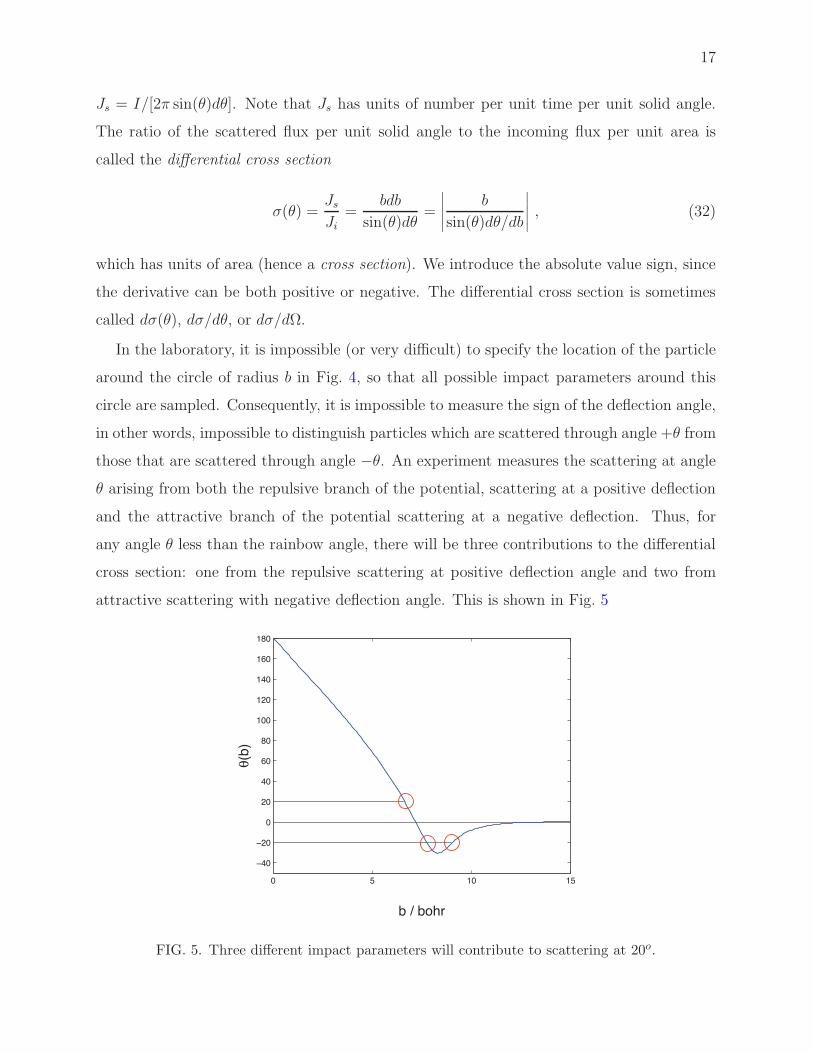
attractive scattering with negative deflection angle. This is shown in Fig. 5
0 5 10 15
−40
−20
0
20
40
60
80
100
120
140
160
180
b / bohr
θ(b)
FIG. 5. Three different impact parameters will contribute to scattering at 20o.

18
For angles greater than the rainbow angle, only the repulsive branch will contribute.
Since the derivative of the deflection function appears in the denominator of the expression
for the differential cross section [Eq. (32)], the largest differential cross sections will occur
for angles at which θ(b) is nearly flat: namely at small deflection angles (forward scattering)
and in the region of the rainbow. Large differential cross sections imply that incoming
flux associated with many impact parameters will all appear at a single (or small range of)
scattering angles.
Figure 6 shows the classical differential cross section (multiplied by sin(θ)) for Ar–Ar
scattering at an energy of 0.002 Hartree. As we will see in the next section, the quantum
treatment will smooth out the classical singularities at θ = 0 and θ = θR. This will give rise
to quantum interference (just like in the classic two-slit experiment [6]).
0 20 40 60 80 100 120 140 160 1800
5
10
15
20
25
30
35
40
45
50
scattering angle / degree
sin(
thet
a) x
dsi
g (b
ohr2
/Sr)
Classical Ar−Ar scattering E = 0.002 Hartree
FIG. 6. Classical differential cross section, Ar–Ar scattering, E = 0.002.
Problem 9
Write a Matlab script to determine the classical differential cross section for the scattering
of two Ar atoms at E = 0.006. You have previously written a script to determine θ(b),
which you can use to obtain θ at a grid of values of b. Now, determine the derivative
dθ/db using the Matlab function gradient, in other words
dth=gradient(th,db);
19
where db is the spacing of your impact parameter grid. Then determine the rainbow
angle
[thr nr]=min(dth);thr=abs(thr);
Here, nr is the point in your array where the rainbow angle occurs. Next define a regular
grid in angle, for example
dang=thr/30;angl=[1:dang:thr];angg=[thr:dang:pi];
Here, angl and angg (angle-lesser and angle-greater) are angular grids for angles less
than and greater than the rainbow angle. Now, determine the range of the three branches
of the deflection function, by executing
n=find(th>0);n=max(n);
Thus, th(1:n) corresponds to the positive branch of the deflection function, th(n+1:nr)
corresponds to the negative branch inside the rainbow angle and th(nr+1:nmax) cor-
responds to the negative branch outside the rainbow angle. Interpolate the differential
cross section from each of these branches onto the regular grid in angle
dcs1=abs(interp1(th(1:n),1./(sin(th(1:n)).*dth(1:n),angl,’cubic’));
dcs2=abs(interp1(th(1:n),1./(sin(th(1:n)).*dth(1:n),angg,’cubic’));
dcs3=abs(interp1(th(n+1:nr),1./(sin(th(n+1:nr)).*dth(n+1:nr),angl,’cubic’));
dcs4=abs(interp1(th(nr+1:nmax),1./(sin(th(nr+1:nmax)).*dth(nr+1:nmax),angl,’cubic’));
Then, add up dcs1, dcs3, and dcs4 to obtain the differential cross section for θ ≤ θR.
The differential cross section for θ > θR is given just by dcs2.
When you plot your result, make sure you multiply by sin θ. This will reduce the size
of the singularities at θ = 0 and θ = π. The value of the dcs in the forward direction
(θ = 0) will still be very large, and dominate everything else on the plot. You can
compensate for this by reducing the range of the y-axis on the plot using the command
plot(x,y,′ylim′,[0 xx]) where xx is the maximum value of y that you wish to display.

20
IV. ELASTIC SCATTERING IN THREE DIMENSIONS: QUANTUM
TREATMENT
A. Separation of radial and angular motion
In three dimensions the relative motion of two spherical particles subject to a poten-
tial which depends only on the magnitude of the distance between them can be reduced
to the motion of the center of mass and the motion of an effective particle of mass µ =
mamb/(ma +mb) (where µ is called the “reduced mass”) in the field of the potential V (r).
The corresponding Schrodinger equation is (outside of the potential, this is exactly the same
as the equation for the motion of the electron in the H atom and the rotational motion of a
diatomic molecule)[
− h2
2µ∇2 + V (r)
]
ψ(r) = Eψ(r) (33)
Because V (r) depends only on the magnitude of the distance between the two particles,
we can expand the wavefunction as
ψ(r) =∑
lm
Ylm(θ, φ)gl(r) =∑
lm
Ylm(θ, φ)Rl(r)/r (34)
where the radial function Rl(r) satisfies the equation (we will drop the subscript l except
when necessary)(
− h2
2µ
d2
dr2+h2l(l + 1)
2µr2+ V (r)
)
R(r) = ER(r) (35)
Here, also, Yl0 is a spherical harmonic, which is related to the regular Legendre polynomial
Pl(cos θ) by
Yl0(θ, φ) =
(
2l + 1
4π
)1/2
Pl(cos θ) (36)
At large r, both the potential V (r) and the centrifugal barrier go to zero, so that the
radial function is the solution to the equation
d2R(r)/dr2 = −k2R(r)
and, thus, can be expressed either as linear combination of sin(kr) and cos(kr), or a linear
combination of exp(ikr) and exp(−ikr). In most cases the potential goes to zero much faster
21
than r2, so that (as in the case of the classical treatment of elastic scattering), it is useful
to consider the behavior of this equation when V (r) is zero, but not the centrifugal barrier.
You can show that in this case we have
limr→∞
Eq. (35) =
[
x2d2
dx2− l(l + 1) + x2
]
R(x) = 0 (37)
where x = kr.
The solutions to this equation are related to the well-known spherical Bessel functions of
the first and second kind: jl(x) and yl(x),[7] which themselves are solutions to the Hemlholz
equation in spherical coordinates, namely
x2d2f
dx2+ 2x
df
dx+[
x2 − l(l + 1)]
fl(x) = 0
where fl(x) is either jl(x) or yl(x).
Problem 10
Show that the Ricatti-Bessel functions
jl(x) = xjl(x)
and
yl(x) = xyl(x)
Satisfy Eq. (37).
The spherical Bessel functions are related to the cylindrical Bessel functions Jn(x) and
Yn(x) through the relation
jl(x) =[
π
2x
]1/2
Jl+ 1
2
(x) (38)
and, for the linearly independent Bessel function of the second kind
yl(x) =[
π
2x
]1/2
Yl+ 1
2
(x) (39)
22
B. Numerical determination of the scattering wavefunction
As r goes to zero, the potential becomes greater than the energy, so that the solution to
the radial Schrodinger equation is either exponentially increasing or exponentially decreasing
as r → 0. We have to take the latter, since the wavefunction has to remain finite.
To obtain R(r) everywhere, we start at small r, with an approximation to the correct
exponentially decreasing function. If we assume that V (r) is constant and large at r = r0,
then we can approximate
R(r0) = 1× 10⁻¹⁰
dR
dr
∣
∣
∣
∣
∣
r=r0
= 1× 10⁻¹⁰κ0 (40)
where κ0 =
2µ [V (r0)− E] /h21/2
If the spacing of our grid is h, then Eq. (40) allows us
to write
R(r1) = R(r0) +dR
dr
∣
∣
∣
∣
∣
r=r0
(r − r0) = (1 + κ0h)× 1× 10⁻¹⁰
Here we implicitly assume that R(r) behaves linearly in the first sector. Once we know the
values of R0 and R1 we can use the Numerov method [Eq. (16)] to obtain R(r) at all larger
values of R.
Problem 11
Write a Matlab script to determine R(r) for the collision of two Ar atoms at E = 0.0005.
You can use the Numerov method to propagate the solution out to large r (probably
r = 20 will be largely sufficient). The mass of Ar is 39.948 amu (the collision reduced
mass is µ = m/2).
At large r, the solution can be written as a linear combination of the two Ricatti-Bessel
functions yl(kr) and jl(kr), namely
limr→∞
R(r) =1
k
[
Aljl(kr) +Blyl(kr)]
(41)

23
Here Al and Bl are two arbitrary constants. Since both A and B are arbitrary, we have
multiplied them both here by 1/k, for convenience later.
If rN−1 and rN are your two last grid points, then you can obtain the coefficients Al
and Bl by solving the set of linear equations (use Matlab’s backslash function)
jl(krN) yl(krN)
jl(krN−1) yl(krN−1)
Al
Bl
=
kR(rN )
kR(rN−1
(42)
You can obtain the values of the Ricatti-Bessel functions at rN and rN−1 using Matlab’s
besselj and bessely commands for the cylindrical Bessel functions. [Remember to
convert these to spherical Bessel functions using Eqs. (38) and (39)].
To check that everything is working, you should find that the values of the expansion
coefficients Al and Bl are converged with respect to decreasing r0, increasing rN , and
increasing the size of the grid. Since the overall normalization of the wavefunction is
arbitrary, we can avoid working with large numbers by renormalizing so that
A =A√
A2 +B2and B =
B√A2 +B2
To test your Matlab code, Tab. III the values of A and B for Ar–Ar scattering at
E=0.0005:
TABLE III. Asymptotic expansion coefficients, Ar–Ar scattering, E=0.0005 hartree.a
l ψ(RN ) Ab Bb Sc
0 1.2708×10⁻⁷ 0.94857 –0.31662 0.79950–0.60067i
30 –5.3398×10⁻⁷ –0.93076 0.36563 0.73263–0.68062i
80 –2.0026×10¹¹ 0.99442 –0.10545 0.97776–0.20972i
a µ = 19.974, r0 = 5.5, rN = 25, h = 0.02.b renormalized.c see Eq. (49)
When the centrifugal barrier becomes very large, so that
hl(l + 1)
2µr2>> V (r)
24
then the Schrodinger equation for R(r) [Eq. (35)] becomes identical to the equation for
the Ricatti-Bessel functions [Eq. (37)]. The solution which behaves correctly at the origin
(limr→0R(r) = 0) is jl(kr). Thus, at large l, the expansion coefficients are liml→∞Al = 1
and liml→∞Bl = 0.
Now, from our numerical solution of the radial Schrodinger equation [Eq. (41)] we see
that the large R behavior of the wavefunction is
limr→∞
ψ(r) =∑
lm
Ylm(θ, φ)R(r)
r=∑
l
1
kr
[
Aljl(krN) +Blyl(krN)]
Yl0(θ, φ)
=∑
l
[Aljl(krN) +Blyl(krN)] Yl0(θ, φ)
=∑
l
[
2l + 1
4π
]1/2
[Aljl(krN) +Blyl(krN)]Pl(cos θ) (43)
Here, we have limited the sum just to the m = 0 projection states, because the scattering
has cylindrical symmetry. By equating Eqs. (68) and (43), we can obtain the coefficients in
the expansion of the scattering amplitude in terms of the coefficients Al and Bl, which we
have obtained numerically.
To do so, we need first examine the asymptotic properties of the Ricatti-Bessel functions.
Since
limx→∞
Jν(x) =[
2
πx
]1/2
cos(
x− 1
2νπ − 1
4π)
so that
limx→∞
Jl+ 1
2
(x) =[
2
πx
]1/2
cos[
x− (l + 1)π
2
]
we find
limx→∞
jl(x) =1
xcos
[
x− (l + 1)π
2
]
(44)
and, similarly (you should show this)
limx→∞
yl(x) =1
xsin
[
x− (l + 1)π
2
]
(45)
Rather than use the real spherical Bessel functions, we can use the complex spherical
25
Hankel functions, namely
h(1,2)l (x) = jl(x)± iyl(x) (46)
where the first (second) spherical Hankel functions corresponds to the plus (minus) sign.
Problem 12
Use Eq. (46) to show that the asymptotic (r → ∞) behavior of these two spherical
Hankel functions is given by
limr→∞
h(1,2)l (kr) =
1
krexp ±i [kr − (l + 1)π/2] =
(∓i)l+1
kre±ikr (47)
Problem 13
The behavior of the Bessel functions at very large r is given by Eqs. (44) and (45). Show
that
limr→∞
R(r)
r=
1
2kr
[
(Al − iBl)h(1)l + (Al + iBl)h
(2)l
]
=1
2
[
(Al − iBl)h(1)l + (Al + iBl)h
(2)l
]
(48)
You can re-arrange this equation to write
limr→∞
R(r)
r= Cl
[
Slh(1)l (kr) + h
(2)l (kr)
]
(49)
where Cl and Sl are complex constants.

26
Problem 14
Determine an expression which relates the constant Sl to the constants Al and Bl which
you obtain from your Numerov propagation.
See if you can derive any limits on the magnitude of the S coefficient Now, from the
answer to Problem 13 we see that
limr→∞
R(r)
r=
1
krC[
(−i)l+1eikrSl + il+1e−ikr]
(50)
Insertion of this equation into Eq. (43) leads to
limr→∞
ψ(r) =∑
lm
Ylm(θ, φ) limr→∞
R(r)
r=∑
l
[
2l + 1
4π
]1/2
Pl(cos θ) limr→∞
R(r)
r
=∑
l
[
2l + 1
4π
]1/21
krC[
(−i)l+1eikrSl + il+1e−ikr]
Pl(cos θ)
=∑
l
[
2l + 1
4π
]1/2i
krC[
−(−i)leikrSl + ile−ikr]
Pl(cos θ) (51)
C. Phase shift
From Eqs. (41), (44), and (45), we see that at large R we can write
limr→∞
R(r) ∼ Al cos[
kr − π
2(l + 1)
]
+Bl sin[
kr − π
2(l + 1)
]
∼ Al sin (kr − lπ/2) +Bl cos (kr − lπ/2) (52)
Equivalently, we can write
limr→∞
R(r) ∼ D sin (kr − lπ/2 + δl) (53)
where δl is the “phase shift”.
27
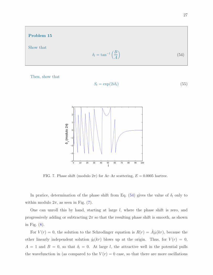
Problem 15
Show that
δl = tan−1(
B
A
)
(54)
Then, show that
Sl = exp(2iδl) (55)
0 10 20 30 40 50 60 70 80 90 100−4
−3
−2
−1
0
1
2
3
l
δ l (m
odul
o 2π
)
FIG. 7. Phase shift (modulo 2π) for Ar–Ar scattering, E = 0.0005 hartree.
In pratice, determination of the phase shift from Eq. (54) gives the value of δl only to
within modulo 2π, as seen in Fig. (7).
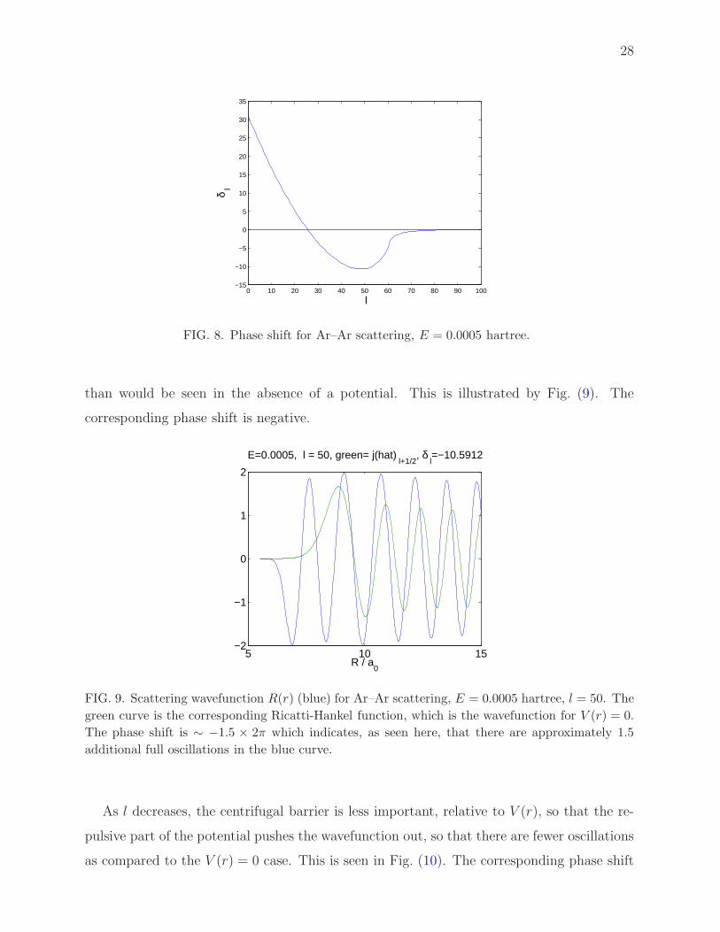
One can unroll this by hand, starting at large l, where the phase shift is zero, and
progressively adding or subtracting 2π so that the resulting phase shift is smooth, as shown
in Fig. (8).
For V (r) = 0, the solution to the Schrodinger equation is R(r) = Ajl(kr), because the
other linearly independent solution yl(kr) blows up at the origin. Thus, for V (r) = 0,
A = 1 and B = 0, so that δl = 0. At large l, the attractive well in the potential pulls
the wavefunction in (as compared to the V (r) = 0 case, so that there are more oscillations
28
0 10 20 30 40 50 60 70 80 90 100−15
−10
−5
0
5
10
15
20
25
30
35
l
δ l
FIG. 8. Phase shift for Ar–Ar scattering, E = 0.0005 hartree.
than would be seen in the absence of a potential. This is illustrated by Fig. (9). The
corresponding phase shift is negative.
5 10 15−2
−1
0
1
2
R / a0
E=0.0005, l = 50, green= j(hat) l+1/2
, δ l=−10.5912
FIG. 9. Scattering wavefunction R(r) (blue) for Ar–Ar scattering, E = 0.0005 hartree, l = 50. The
green curve is the corresponding Ricatti-Hankel function, which is the wavefunction for V (r) = 0.
The phase shift is ∼ −1.5 × 2π which indicates, as seen here, that there are approximately 1.5
additional full oscillations in the blue curve.
As l decreases, the centrifugal barrier is less important, relative to V (r), so that the re-
pulsive part of the potential pushes the wavefunction out, so that there are fewer oscillations
as compared to the V (r) = 0 case. This is seen in Fig. (10). The corresponding phase shift
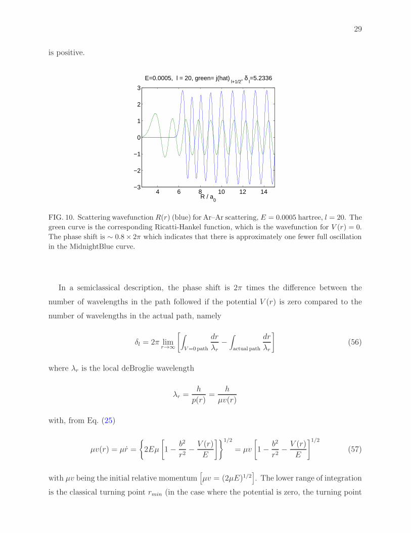
29
is positive.
4 6 8 10 12 14−3
−2
−1
0
1
2
3
R / a0
E=0.0005, l = 20, green= j(hat) l+1/2
, δ l=5.2336
FIG. 10. Scattering wavefunction R(r) (blue) for Ar–Ar scattering, E = 0.0005 hartree, l = 20. The
green curve is the corresponding Ricatti-Hankel function, which is the wavefunction for V (r) = 0.
The phase shift is ∼ 0.8 × 2π which indicates that there is approximately one fewer full oscillation
in the MidnightBlue curve.
In a semiclassical description, the phase shift is 2π times the difference between the
number of wavelengths in the path followed if the potential V (r) is zero compared to the
number of wavelengths in the actual path, namely
δl = 2π limr→∞
[
∫
V=0path
dr
λr−∫
actual path
dr
λr
]
(56)
where λr is the local deBroglie wavelength
λr =h
p(r)=
h
µv(r)
with, from Eq. (25)
µv(r) = µr =
2Eµ
[
1− b2
r2− V (r)
E
]1/2
= µv
[
1− b2
r2− V (r)
E
]1/2
(57)
with µv being the initial relative momentum[
µv = (2µE)1/2]
. The lower range of integration
is the classical turning point rmin (in the case where the potential is zero, the turning point
30
is equal to the impact parameter) so that
δl =µv
h
∫ R
b
[
1− b2
r2
]1/2
dr −∫ R
rmin
[
1− b2
r2− V (r)
E
]1/2
dr
(58)
Here, R is the value of the distance for which the potential has effectively vanished (see
Sec. II.B). The first integral can be evaluated analytically to give [8]
∫ R
b
[
1− b2
r2
]1/2
dr =(
R2 − b2)1/2 − b cos−1(b/R)
In order to evaluate numerically both integrals, we need to know the correspondence be-
tween the classical impact parameter and the quantum mechanical angular momentum. We
remember from Eq. (23) that l2cl = (µvb)2. We also know that square of the angular mo-
mentum in quantum mechanics is⟨
l2⟩
= l(l+1)h2. Thus, in Eq. (58) we need to replace b2
by
b2 =h2l(l + 1)
(µv)2
Thus, Eq. (58) becomes (in atomic units, where h = 1)
δl = µv
∫ R
b
[
1− l(l + 1)
µvr2
]1/2
dr −∫ R
rmin
[
1− l(l + 1)
(µvr)2− V (r)
E
]1/2
dr
= µv
(
R2 − b2)1/2 − b cos−1
(
b
R
)
−∫ R
rmin
[
1− l(l + 1)
(µvr)2− V (r)
E
]1/2
dr
= µv
(
R2 − b2)1/2 − b cos−1
(
b
R
)
−∫ R
rmin
[
1− b2
r2− V (r)
E
]1/2
dr
(59)
where, here b = [l(l + 1)]1/2/µv.
Problem 16
Write a Matlab script to determine the semiclassical phase shift, defined in the preceding
equation. Use the work you did in Problem 6 to determine the turning point, then use
the Matlab function quad to evaluate the integral.
For Ar–Ar collisions at E = 0.0005 hartree, the semiclassical phase shift, as a function of

31
l, differs only minutely from the quantum phase shift shown in Fig. (8). The following table
contains some numerical comparisons.
TABLE IV. Comparison of quantum and semi-classical phase shifts (radians) for Ar–Ar scattering,
E=0.0005 hartree.
l δQ [Eq. (54)] δSC [Eq. (59)]
0 31.09 31.87
20 5.23 5.23
40 –9.06 –9.07
60 –4.89 –5.01
Typically, semi-classical approximations become less accurate when the mass is reduced.
If we replace the mass of Ar with that of He, and simulate He–He collisions at E = 0.0005
hartree with the Ar–Ar potential, the reduced mass drops form ∼ 20 to ∼ 2, a factor of 10.
However, as shown by Fig. 11 the agreement is still excellent, with a few slight exceptions,
notably at l = 0.
0 5 10 15 20 25 30−5
0
5
10
15
l
δ l
FIG. 11. Phase shift for He–He scattering with the Ar–Ar potential, E = 0.0005 hartree. The Mid-
nightBlue curve is the quantum predictions from Eq. (54) and the green circles are the semiclassical
predictions from Eq. (59). Note that the minimum occurs at l ∼= 15, while the minimum in Fig. (8)
occurs at l ∼= 50. This is because for a lighter reduced mass the value of l which corresponds to a
given impact parameter is smaller.

32
D. Scattering boundary conditions
The Schrodinger equation is solved subject to the boundary condition
limr→∞
ψ(r) = eikz +f(θ)eikr
kr(60)
The first term corresponds to an incoming plane wave and the second term, to the scattered
wave. [9]
The flux density can be evaluated as
~J = − ih
2µ(ψ∗∇ψ − ψ∇ψ∗) (61)
The incoming flux is evaluated by using ψi = eikz which yields
Jiz =hk
µz
This is the incoming flux per unit area (dA = dxdy). The outgoing flux through a sphere of
radius r can be evaluated by using ψo = f(θ)eikr/r and knowing that the radial component
of the gradient in spherical polar coordinates is
rd
dr
This yields
Jor =
(
h
kµ|f(θ)|2/r2
)
r (62)
The total outgoing flux through the surface of a sphere of radius r is
∫
Jor2dΩ
Since the scattering is independent of the azimuthal angle (by symmetry) we see that the
outgoing flux per unit solid angle is
Jo(Ω) =h
kµ|f(θ)|2
33
Since the differential cross section is defined (see Sec. III) as the ratio of the outgoing flux
per unit solid angle to the incoming flux per unit area, we see that
dσ
dΩ≡ Jo/Ji =
|f(θ)|2k2
(63)
The quantity f(θ) is called the “scattering amplitude.”
E. Determination of f(θ)
To obtain the scattering amplitude, we first use the well-known expansion of a plane wave
in spherical waves (due originally to Lord Rayleigh) namely
eikz =∑
l
il [4π(2l + 1)]1/2 jl(kr)Yl0(θ, φ) (64)
where we see the spherical Bessel function one more time. From Eq. (36), we see that
Eq. (64) can be rewritten in terms of Legendre polynomials as
eikz =∑
l
il(2l + 1)jl(kr)Pl(cos θ) (65)
Similarly, we can expand the scattering amplitude in a Legendre series
f(θ) =∑
l
1
2(2l + 1)flPl(cos θ) = i
∑
l
1
2i(2l + 1)flPl(cos θ) (66)
Because of the orthogonality properties of the Legendre polynomials
∫ π
0Pl(cos θ)Pm(cos θ) sin θdθ =
2δlm2l + 1
(67)
we see that
fl =∫ π
0Pl(cos θ)f(θ) sin θdθ
Consequently, the asymptotic behavior of the wavefunction [Eq. (60)] can be re-expressed
as
34
limr→∞
ψ(r) =∑
l
(2l + 1)
[
1
2fleikr
kr+ iljl(kr)
]
Pl(cos θ) (68)
From Eq. (46) we see that
jl(kr) =1
2
[
h(1)l (kr) + h
(2)l (kr)
]
With this, along with Eq. (47), we can rewrite Eq. (68) as
limr→∞
ψ(r) =1
2
i
kr
∑
l
(2l + 1)
[
eikr(
fli− 1
)
+ (−1)le−ikr
]
Pl(cos θ) (69)
Problem 17
Check all the algebra and derivations. Now, the asymptotic expression for the wave-
function you have obtained by numerical solution [Eq. (51)] must equal this expression.
Knowing this, for each l equate the coefficients of exp(ikr) and exp(−ikr) in Eqs. (51)
and (69) to derive an equation for the terms fl in the expansion of the scattering am-
plitude in terms of the coefficient Sl. By requiring that the coefficients of exp(−ikr) beidentical in Eqs. (51) and (69), you can show that
Cl = il [(2l + 1)π]1/2 (70)
and
fl = i(1− Sl) (71)
Requiring the coefficient of exp(−ikr) to be identical, yields Eq. (71).
Problem 18
Modify your Matlab script to obtain as a function of l the scattering amplitude from this
equation at all values of l. As l increases, Sl goes to +1, so that liml→∞ fl = 0. Then,

35
using Eq. (63) determine the differential cross section for Ar–Ar scattering at E=0.0005.
Do a similar calculation for He–He scattering (µ = 2.0013 amu) described by the Ar–Ar
potential. In both cases, compare your results with the classical differential cross section
plotted in Fig. 6.
Table V lists some Ar–Ar scattering amplitudes
TABLE V. Comparison of quantum scattering amplitudes and differential cross section for Ar–Ar
scattering, E=0.0005 hartree, lmax=100.
θ f(θ) dσ/dΩ a
2 1.0522e+3 + 9.5366e+1 i 30655
22 5.5310e+1 + 6.1524e+1 i 187.98
42 –4.0047e+1 + 3.1983e+1 i 72.14
62 –1.4737e+1 + 2.8595e+1 i 28.42
a Eq. (63); Units of a20/Sr.
Here is a plot of the differential cross sections for Ar–Ar and for He–He (with the Ar–Ar
potential).
0 20 40 60 80 100 120 140 160 1800
50
100
150
200
250
300
350
400
450
500
θ / degrees
sinθ
dσ/
dθ /
Ang
2 /Sr
FIG. 12. Differential scattering of two Ar atoms, E = 0.0005 hartree.

36
0 20 40 60 80 100 120 140 160 1800
50
100
150
200
250
300
θ / degrees
sinθ
dσ/
dθ/S
r
FIG. 13. Differential scattering of two He atoms, E = 0.0005 hartree.
F. Integral Cross Section
The integral over all solid angle of the differential cross section defines the “integral”
cross section, namely
σ =∫
dσ
dΩsin θdθdφ = 2π
∫
dσ
dΩsin θdθ =
2π
k2
∫
|f(θ)|2 sin θdθ =
Here, because the scattering is azimuthally symmetric, we have integrated trivially over φ.
Problem 19
Show that if you substitute the expansion over l of f(θ) [Eq. (66)] and use the orthogo-
nality of the Legendre polynomials [Eq. (67)], you obtain
σ =π
k2∑
l
(2l + 1)|fl|2 =π
k2∑
l
(2l + 1)|1− Sl|2 (72)
Using Eqs. (55), show that this is equivalent to
σ =2π
k2∑
l
(2l + 1) sin2 δl (73)
Then, use this equation, as well as Eqs. (55), (66), and the relationship Pl(θ = 0) = 1
to prove the “optical theorem” which states that the integral cross section is proportional
37
to the imaginary part of the amplitude for scattering in the forward (θ = 0) direction.
[10]
σ =4π
k2Im[f(θ = 0)] (74)
V. INELASTIC SCATTERING
A. Generalities
Suppose you scatter an atom with internal states ψi, which satisfy the Schrodinger equa-
tion
Hint(q)χn(q) = εnχn(q) (75)
where q designates the internal degrees of freedom and εn is the internal energy of state n.
The eigenfunctions χn(q) are, of course, orthonormal, namely
∫
χ∗n(q)χm(q)dq = δmn
The corresponding time-independent Schrodinger equation for the system of the atom plus
a structureless collision partnerthen becomes
[
− h2
2µ∇2 +H(r, q)
]
ψ(r, q) = Eψ(r,q) (76)
where H(r, q) is some Hamiltonian which depends on both the separation of the atom with
its collision partner and the internal degrees of freedom of the atom. We shall assume for
simplicity here that H depends only the the magnitude of r, not its orientation. In the limit
of large separation,
limr→∞
H(r, q) = Hint(q) (77)
Similarly, the wavefunction depends on both the internal degree(s) of freedom and the
38
separation coordinate r. Extending Eq. (??), we will expand the wavefunction as
ψ(r, q) =∑
n
∑
lm
Ylm(θ, φ)gln(r)χn(q) =∑
n
∑
lm
Ylm(θ, φ)Cln(r)
rχn(q) (78)
Now, substitute this expansion into Eq. (76), then premultiply by one of the internal state
functions, χm(q), say, and integrate over q. You can show that the Schrodinger equation is
then transformed into a set of coupled ordinary differential equations
[
− h2
2µ
d2
dr2+h2l(l + 1)
2µr2+ Vmm(r)− E
]
Cm(r) = −∑
n 6=m
Vmn(r)Cn(r) , (79)
where
Vmn(r) =∫
χ∗m(q)H(r, q)χn(q)dq (80)
Note that for convenience in the notation later in the section we are using C(r) rather than
R(r) to designate the radial wavefunctions divided by r.
Formally, we can rewrite these so-called “close-coupled” equations as
[
Id2
dr2+W(r)
]
C(r) = 0 (81)
where
W(r) = 2µ [EI−V(r)] (82)
In this equation, and henceforth, we use atomic units, where h = 1.
The solution to Eq. (81) is a matrix, with each column representing a linearly independent
solution involving coefficients Cnm for all n internal states. For the case where there are only
two internal states,
C(r) =
C11(r) C12(r)
C21(r) C22(r)
(83)
Equation (77) implies that asymptotically the W(r) matrix is diagonal with elements
limr→∞
Wnn(r) = k2n ≡ 2µ
[
E − εn −l(l + 1)
R2
]
(84)
The appropriate scattering boundary conditions in this two-channel case is
39
limr→∞
C(r) =
k−1/21 h
(2)l1(k1r) 0
0 k−1/22 h
(2)l2(k2r)
−
k−1/21 h
(1)l1(k1r) 0
0 k−1/22 h
(1)l2(k2r)
S (85)
Here the S coefficient is now an S matrix. In matrix notation, Eq. (85) is
limr→∞
C(r) = h(2)(r)− h(1)(r)S (86)
In the case where the angular momentum l is zero, Eq. (85) goes to
limr→∞
C(r) = i
k−1/21 exp(−ik1r) 0
0 k−1/22 exp(−ik2r)
+ i
k−1/21 exp(ik1r) 0
0 k−1/22 exp(ik2r)
S (87)
B. The renormalized Numerov method in the asymptotic basis
Given the potential, how do we obtain the S matrix? We set up a regular grid of N + 1
points, with h the width of each sector. At the first point, which is presumed to lie well
within the classically forbidden region, we will assume that the wavefunction vanishes, in
other words
C(r0) ≡ C0 =
0 0
0 0
(88)
To propagate the solution we can use the Numerov algorithm [Eq. (16)], namely (for a
one-dimensional problem)
(1− TM+1)CM+1 = (2 + 10TM)CM − (1− TM−1)CM−1 (89)
40
where
TM = −h2
12W (rM) = −h
2
122µ [E − V (r = rM)] (90)
Because the kinetic energy is diagonal, this same three-term recursion relation can be easily
generalized to multidimensional problems. Note the difference between Eq. (16) and (89). In
the former case the T terms are defined asE−V , whereas here, to be consistent with Ref. [11],
we define the T terms as V − E. For a multi-state (sometimes called “multichannel”)
problem, Eqs. (89) and (90) are written in matrix notation, namely
(I−TM+1)CM+1 = (2I+ 10TM)CM − (I−TM−1)CM−1 (91)
and
TM = −h2
122µ [EI−V(r = rM)] (92)
In order to avoid the numerical instabilities caused by exponentially growing solutions in
the classically forbidden region, we shall use the “renormalized” Numerov algorithm, due to
Johnson. [12] To derive the propagation algorithm, we introduce two transformations. First,
we define
FM = (I−TM)CM (93)
so that the basic propagation relation [Eq. (89)] becomes
FM+1 −UMFM + FM−1 = 0 (94)
where
UM = (2I+ 10TM) (I−TM)−1 (95)
Note that we will use subscript “M” to designate the M th sector or the M th grid point RM ,
while we use subscripts n and m as as row and column indices.
Now, we define the “ratio matrix”
RM+1 = FM+1F−1M = (I−TM+1)CM+1 [(I−TM)CM ]−1 (96)
It follows that FM+1 = RM+1FM and R−1M = FM−1F
−1M . Solving for R rather than C
will eliminate instabilities in the original Numerov method due to exponentially growing
41
solutions in the classically forbidden region.
This allows you to rewrite the equation for the ratio matrix [Eq. (96)] as
RM+1 = UM −R−1M (97)
This is a two-term recursion relation for the ratio matrix.
Propagation of the ratio matrix can be accomplished provided we specify the inverse of
R at the first grid point, namely R−10 . To do so we assume that the solution at the first grid
point vanishes [Eq. (88)]. At the second grid point, the solution will be small but not zero.
Consequently, F0 = 0 and F1 6= 0. This implies that R−10 = 0. Thus,
R1 = U0 (98)
and
R2 = U1 −R−11 = U1 −U−1
0 (99)
Subsequently, the two-term recursion relation [Eq. (97)] can be used to determine the ratio
matrix all the way until the last grid point.
Since W is symmetric, it follows that both T and U are symmetric. Since R−10 = 0,
which is symmetric, the R matrix continues to be symmetric throughout the propagation.
We can also show that [see Eq. (95)],
UM = (2I+ 10TM) (I−TM)−1 = 12(I−TM)−1 − 10I (100)
This along with Eq. (97) define the propagation from grid point M to grid point M + 1.
Knowing the ratio matrix at grid point M (RM), as well as UM from Eq. (100), we can
compute RM+1. The overall propagation relation is then
RM+1 = −R−1M + 12 (I−TM)−1 − 10I
= −R−1M + 12
(
I+h2
12WM
)−1
− 10I (101)
This involves two matrix inversions per sector.
42
Problem 20
Show that if we assume F0 = 0 and F1 6= 0, then R−10 = 0.
C. Determination of the log-derivative matrix
Extraction of the S matrix is most easily done if one first determines the log-derivative
matrix at the end of the last sector. This is defined as a multi-channel generalization of the
logarithmic derivative of the wavefunction, namely
YN = CN′C−1
N
For this we will need the derivative of the solution. We know, by application of a standard
Taylor expansion,
ψ(r + h) = ψ(r) + hdψ
dr
∣
∣
∣
∣
∣
r
+h2
2
d2ψ
dr2
∣
∣
∣
∣
∣
r
+h3
6
d3ψ
dr3
∣
∣
∣
∣
∣
r
and, similarly
ψ(r − h) = ψ(r)− hdψ
dr
∣
∣
∣
∣
∣
r
+h2
2
d2ψ
dr2
∣
∣
∣
∣
∣
r
− h3
6
d3ψ
dr3
∣
∣
∣
∣
∣
r
By subtracting these two equations you can obtain
dψ
dr
∣
∣
∣
∣
∣
r=rN
≈ ψN+1 − ψN−1
2h− h2
6
d3ψ
dr3
∣
∣
∣
∣
∣
r=rN
+O
h5d5ψ
dr5
∣
∣
∣
∣
∣
r=rN
(102)
Nowd3ψ
dr3
∣
∣
∣
∣
∣
r=rN
≈ ψ′′N+1 − ψ′′
N−1
2h=
−WN+1ψN+1 +WN−1ψN−1
2h
Here we have used Eq. (81) to simplify the right hand side of the last equation.
We can neglect the terms of O(h5) to obtain
dψ
dr
∣
∣
∣
∣
∣
r=rN
≈ 1
2h(ψN+1 − ψN ) +
h
12(WN+1ψN+1 −WN−1ψN−1)
43
=1
h
[(
1
2+h2
12WN+1
)
ψN+1 −(
1
2+h2
12WN−1
)
ψN−1
]
=1
h
[(
1
2− TN+1
)
ψN+1 −(
1
2− TN−1
)
ψN−1
]
(103)
We can generalize this to our matrix representation of the solution in the case of coupled
equations obtaining
CN′ =
1
h
[(
1
2I−TN+1
)
CN+1 −(
1
2I−TN−1
)
CN−1
]
(104)
The derivation of the formula for the derivative in Eq. (103) was first given by Blatt [13]
and follows closely the procedure used in deriving the original Numerov method. [14]
At the end of the last sector we obtain RN+1 from R−1N . We know that
RN+1 = FN+1F−1N = (I−TN+1)CN+1 [(I−TN)CN ]
−1
and
RN = FNF−1N−1 = (I−TN )CN [(I−TN−1)CN−1]
−1
From the first of these two equations we obtain
CN+1 = (I−TN+1)−1
RN+1 (I−TN)CN
and from the second, we obtain
CN−1 = (I−TN−1)−1
R−1N (I−TN )CN
If we substitute these two equations into Eq. (104), and then post multiply by C−1N , we
obtain the following expression for the log-derivative matrix at r = rN
YN∼= 1
h
[(
1
2I−TN+1
)
(I−TN+1)−1
RN+1 −(
1
2I−TN−1
)
(I−TN−1)−1
R−1N
]
(I−TN)
(105)

44
D. Operational outline of the renormalized Numerov method
Figure 14 shows the division of the r axis into N sectors, starting at r = r0. Sector M
is delimited by r = rM−1 to the left and r = rM to the right. The renormalized Numerov
sector 1 2
r0 r2r1 rN–2 rNrN-1
N–1 N
rN+1
FIG. 14. Schematic partition of the r-axis into a series of sectors. The last sector ends at r = rN .
To determine the log-derivative matrix at r = rN , we need to propagate one more step, out to
r = rN + h.
method proceeds by determining at the left-hand side of sector M , in order, V(rM−1),
W(rM−1), T(rM−1) and U(rM−1), and then, with this information, transforming the ratio
matrix at the left of sector M (RM−1) into the ratio matrix at the right of this same sector
(RM). In this way the ratio matrix at r = rM−1 is propagated to r = rM .
At the end of the numerical propagation we have to carry out one more propagation step,
out to r = rN+1 (see Fig. 14). Then we use the ratio matrix at the right end-point of the
last sector (RN), as well as the T matrices at r = rN−1, r = rN , and r = rN+1 and the
ratio matrix at the supplemental point r = rN+1 to determine, by means of Eq. (105) the
log-derivative matrix at r = rN .
The operational outline of the renormalized Numerov propagation is as follows:
a. At the first integration point (r = r0) determine W0 and then T0 = −h2
12W0.
b. Determine U0 from Eq. (100) for M = 0.
c. Determine the ratio matrix R1 from Eq. (98). Also calculate the T matrix at the right-
hand side of the first sector (T1).
Then repeat for r = r1 → rN (sectors 2, 3, . . . , N) replacing steps a− c with
b′. Determine UM−1 from Eq. (100)
c′. Determine the new ratio matrix RM by use of Eq. (97), specifically RM = UM−1−R−1M−1.
Also calculate the T matrix at the right-hand side of the current sector (TM).
d. At the end of each sector, update the T and R matrices, namely
TM−1 → TM−2 TM → TM−1 RM → RM−1

45
e. Upon finishing the N th sector, we carry out one more repetition of steps b′ and c′, out to
rN+1 = rN + h.
e. When propagation is completed, we have calculated TN−1, TN , TN+1 as well as RN ,
and, finally, RN+1. We use these matrices to determine, from Eq. (105), the log-derivative
matrix at r = rN (YN).
E. Determination of the S matrix
We know from Eq. (86) that
limr→∞
C(r) = h(2)(r)− h(1)(r)S (106)
Differentiation gives
limr→∞
C(r)′ = h(2)(r)′ − h(1)(r)′S (107)
where h(1,2)(r)′ are diagonal matrices, with elements given by the derivatives of the diagonal
elements in Eq. (85). From the preceding two equations, we see that
limr→∞
Y(r) = Y(rN) = YN =[
h(2)(rN)′ − h(1)(rN )
′S] [
h(2)(rN)− h(1)(rN)S]−1
(108)
This equation can be rearranged to yield
[
h(1)(rN)′ −Y(rN)h
(1)(rN )]
S =[
h(2)(rN)′ −Y(rN)h
(2)(rN)]
(109)
Since we have previously determined Y(rN), we can solve this set of complex linear equations
for the S matrix. Alternatively, the linear equations can be decomposed into real and
imaginary parts, which you can solve using real (rather than complex) arithmetic for the
real and imaginary parts of S.
If the angular momentum l is zero, then the elements of the diagonal h(1,2)(r) matrices
are
h(1,2)nn (r) = (∓i)k−1/2n exp(±iknr) (110)
where the upper sign goes with the h(1) matrix [see Eq. (87)].
46
Problem 21
Demonstrate the expansion of the wavefunction of Eq. (78) reduces the Schrodinger
equation (76) to the set of coupled ordinary differential equations of Eq. (79).
Problem 22
Show that introduction of the ratio matrix [Eq. (96)] allows you to transform the matrix
Numerov equation (94) into the matrix equation for R, namely Eq. (97).
Problem 23
Demonstrate that Eq. (102) follows from subtraction of the two equations which precede
it.
Problem 24
Show how the overall propagation equation in the renormalized Numerov method (101)
follows from the equations which precede it.
Problem 25
Show how Eq. (109) follows from Eq. (108).
Problem 26
47
Immediately after Eq. (109) we mention that you can obtain the real and imaginary
parts of S separately, by solution of two sets of linear equations each of which involve
only real quantities. Derive these equations.
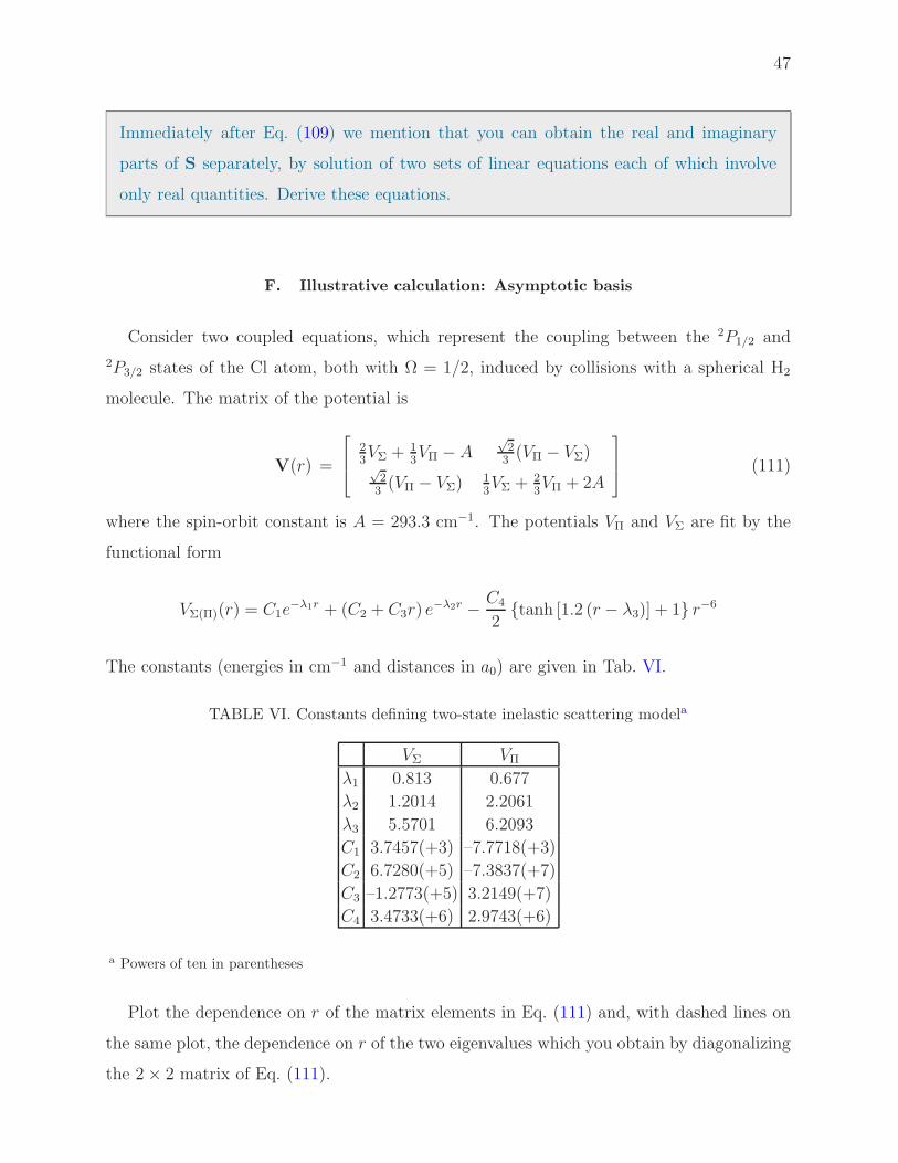
F. Illustrative calculation: Asymptotic basis
Consider two coupled equations, which represent the coupling between the 2P1/2 and
2P3/2 states of the Cl atom, both with Ω = 1/2, induced by collisions with a spherical H2
molecule. The matrix of the potential is
V(r) =
23VΣ + 1
3VΠ − A
√23(VΠ − VΣ)
√23(VΠ − VΣ)
13VΣ + 2
3VΠ + 2A
(111)
where the spin-orbit constant is A = 293.3 cm−1. The potentials VΠ and VΣ are fit by the
functional form
VΣ(Π)(r) = C1e−λ1r + (C2 + C3r) e
−λ2r − C4
2tanh [1.2 (r − λ3)] + 1 r−6
The constants (energies in cm−1 and distances in a0) are given in Tab. VI.
TABLE VI. Constants defining two-state inelastic scattering modela
VΣ VΠλ1 0.813 0.677
λ2 1.2014 2.2061
λ3 5.5701 6.2093
C1 3.7457(+3) –7.7718(+3)
C2 6.7280(+5) –7.3837(+7)
C3 –1.2773(+5) 3.2149(+7)
C4 3.4733(+6) 2.9743(+6)
a Powers of ten in parentheses
Plot the dependence on r of the matrix elements in Eq. (111) and, with dashed lines on
the same plot, the dependence on r of the two eigenvalues which you obtain by diagonalizing
the 2× 2 matrix of Eq. (111).
48
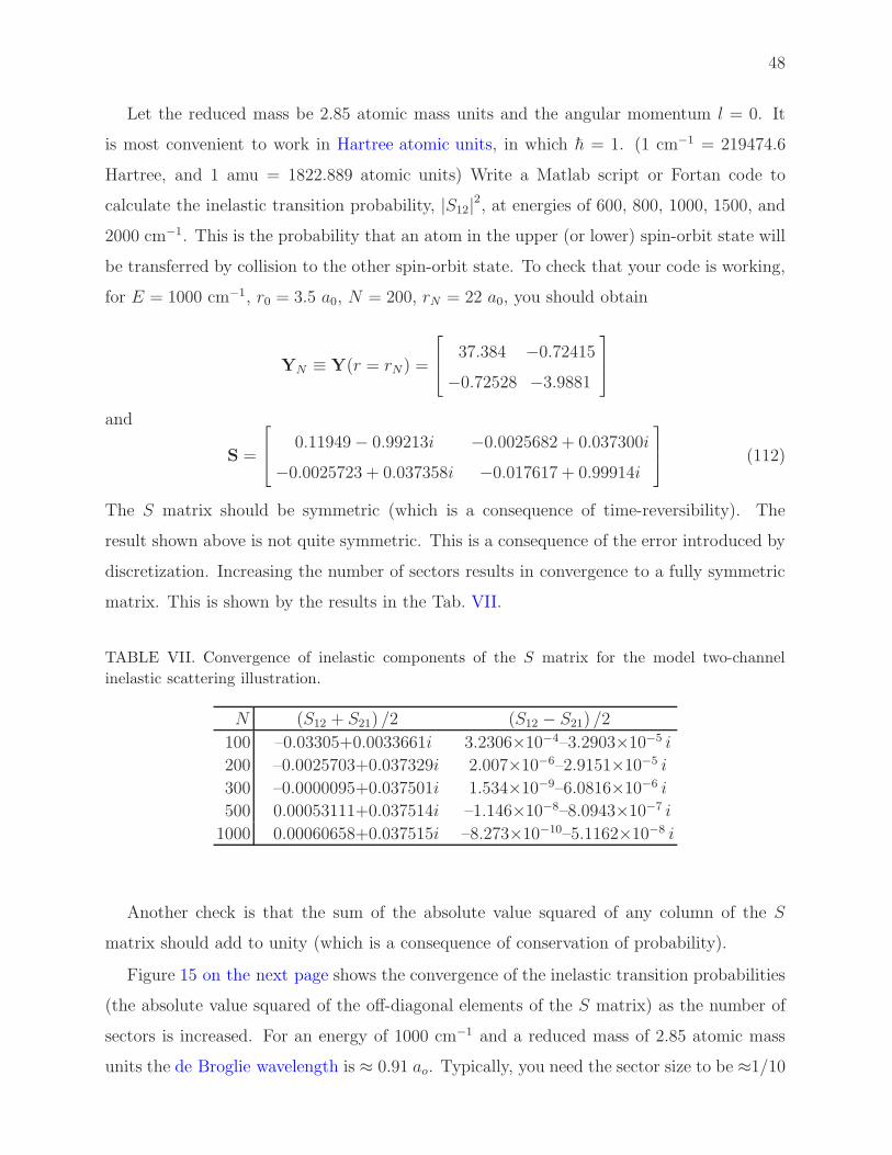
Let the reduced mass be 2.85 atomic mass units and the angular momentum l = 0. It
is most convenient to work in Hartree atomic units, in which h = 1. (1 cm−1 = 219474.6
Hartree, and 1 amu = 1822.889 atomic units) Write a Matlab script or Fortan code to
calculate the inelastic transition probability, |S12|2, at energies of 600, 800, 1000, 1500, and2000 cm−1. This is the probability that an atom in the upper (or lower) spin-orbit state will
be transferred by collision to the other spin-orbit state. To check that your code is working,
for E = 1000 cm−1, r0 = 3.5 a0, N = 200, rN = 22 a0, you should obtain
YN ≡ Y(r = rN) =
37.384 −0.72415
−0.72528 −3.9881
and
S =
0.11949− 0.99213i −0.0025682 + 0.037300i
−0.0025723 + 0.037358i −0.017617 + 0.99914i
(112)
The S matrix should be symmetric (which is a consequence of time-reversibility). The
result shown above is not quite symmetric. This is a consequence of the error introduced by
discretization. Increasing the number of sectors results in convergence to a fully symmetric
matrix. This is shown by the results in the Tab. VII.
TABLE VII. Convergence of inelastic components of the S matrix for the model two-channel
inelastic scattering illustration.
N (S12 + S21) /2 (S12 − S21) /2
100 –0.03305+0.0033661i 3.2306×10⁻⁴–3.2903×10⁻⁵ i
200 –0.0025703+0.037329i 2.007×10⁻⁶–2.9151×10⁻⁵ i
300 –0.0000095+0.037501i 1.534×10⁻⁹–6.0816×10⁻⁶ i
500 0.00053111+0.037514i –1.146×10⁻⁸–8.0943×10⁻⁷ i
1000 0.00060658+0.037515i –8.273×10⁻¹⁰–5.1162×10⁻⁸ i
Another check is that the sum of the absolute value squared of any column of the S
matrix should add to unity (which is a consequence of conservation of probability).
Figure 15 on the next page shows the convergence of the inelastic transition probabilities
(the absolute value squared of the off-diagonal elements of the S matrix) as the number of
sectors is increased. For an energy of 1000 cm−1 and a reduced mass of 2.85 atomic mass
units the de Broglie wavelength is ≈ 0.91 ao. Typically, you need the sector size to be ≈1/10

49
50 100 150 200 250 300 350 4000
0.5
1
1.5x 10
−3
N
1 →
2 tr
ansi
tion
prob
abili
ty
FIG. 15. Convergence of the inelastic transition probability for the model two-channel inelastic
scattering illustration.
the deBroglie wavelength for the numerical integration to be accurate. Here that translates
to a sector size of ≈ 0.09 ao, or ≈ 200 sectors to cover the range 3.5 ≤ r ≤ 22. We see from
Fig. 15 that even with ≈ 150 sectors the calculated inelastic probabilities have converged to
within 1 %.
G. Using the renormalized Numerov method in the locally adiabatic basis
An alternative solution scheme involves propagating in a locally adiabatic basis (see also
Ref. [14]). We refer the reader back to Fig. 14 on page 44. Let VM be the matrix of the
potential [Eq. (80)] at r = rM , namely VM ≡ V(rM) . Then, let XM be the matrix which
diagonalizes VM , namely
XTM V(rM)XM = XT
M VM XM = vM (113)
where vM is the diagonal matrix of the eigenvalues. Since the matrix of the potential
is either symmetric (or Hermitian), the matrix X will define an orthogonal (or unitary)
transformation. We shall assume that V is a real, symmetric matrix. Hereafter, we use
the superscript tilde to designate quantities in the locally adiabatic basis. The columns of
the matrix XM are the linear combinations of the functions χ(q) in which the matrix of

50
H(r, q) is diagonal at r = rM . We will designate these functions φM(q), so that
φM = XTM χ
Here, both φM(q) and χ(q) are column vectors.
The goal is to obtain the matrix C(r) which is a set of linearly-independent combinations
of the internal states χ(q) which solve Eq. (81). The renormalized Numerov method works
by propagating the ratio matrix which [as seen in Eq. (96)] is related to a product of the
solution matrix C at one point and the inverse of the solution matrix at the previous point.
Now, suppose we chose to propagate the solution in the locally adiabatic basis. In this ap-
proach we will seek, in each sector, the matrix CM(r) which is the set of linearly-independent
combinations of the locally adiabatic states φM which are solutions to the CC equations.
For simplicity, we shall suppress the variable q unless needed. In the preceding sections, we
considered solution of the close-coupled equations in the asymptotic basis χ.
Obviously, the CM(r) matrix is related to the CM(r) matrix by the transformation XM .
The application of the renormalized Numerov method in the locally-adiabatic basis will
require first working through the algebra associated with propagating the ratio matrix in
the locally-adiabatic basis. At first thought this seems like a more cumbersome way to solve
the equations, especially since matrix diagonalization is required at each additional grid
point. However, it will offer some advantages, particularly if one is interested in determining
cross sections for scattering at a large number of collision energies or if one has access to
computational hardware and vector libraries which permit a high degree of parallelization.
Propagation in the locally adiabatic basis will make use of the locally-adiabatic equivalent
of the FM matrix of Eq. (93), which we will designate by the superscript tilde, namely
FM =(
I− TM
)
CM (114)
where
TM = XTMTMXM (115)
Now, since CM = XTMCM and since I = XT
M I XM , we can rearrange Eq. (114) as
FM =(
I− TM
)
CM = XTM (I−TM)XMCM = XT
M (I−TM)CM (116)
51
Comparing the right-hand side with Eq. (93), we conclude that
FM = XTMFM (117)
This demonstrates that the F matrix transforms as the basis functions. This is reasonable,
since [Eq. (114)] reveals that F is just a linear combination of the solutions C.
The Numerov propagation relation in the asymptotic basis is given by Eq. (94), which
we repeat here:
FM+1 −UMFM + FM−1 = 0 (118)
Using Eq. (117) to transform the three F matrices into the locally adiabatic basis, we find
XM+1FM+1 = UMXM FM −XM−1FM−1 (119)
We then postmultiply by F−1M and premultiply by XT
M to get
XTMXM+1FM+1F
−1M = XT
MUMXM −XTMXM−1FM−1F
−1M (120)
Now, the overlap between the locally-adiabatic functions in sector M and those in sector
M + 1 is
OM,M+1 = XTMXM+1 (121)
so that the preceding equation can be written as
OM,M+1FM+1F−1M = XT
MUMXM −OTM−1,M FM−1F
−1M (122)
If we define the ratio matrix in the locally-adiabatic basis as
RM ≡ OM−1,M FM F−1M−1 (123)
then Eq. (122) becomes
RM+1 = XTMUMXM −OT
M−1,MR−1M OM−1,M
52
= UM −OTM−1,MR−1
M OM−1,M (124)
where UM is the transform of the UM matrix into the locally adiabatic basis. Now, we
remember that
UM = (2I+ 10TM) (I−TM)−1
Premultiplying by XTM , postmultiplying by XM , and inserting a factor of I = XMXT
M
immediately after the term (2I+ 10TM) gives
XTMUMXM = XT
M (2I+ 10TM)XMXTM (I−TM)−1
XM
= XTM (2I+ 10TM)XM
[
XTM (I−TM)XM
]−1(125)
We recall that the T matrix is defined by Eq. (92). Since the V matrix is diagonalized
by the X matrix, it follows that the T matrix is also diagonalized, with elements
(
TM
)
nn= −h
2
122µ [E − vn(r = rM)] (126)
Consequently, we conclude from Eq. (125) that the UM matrix is also diagonal, namely
XTMUMXM = uM
with elements
(uM)nn =[
2 + 10(
tM)
nn
]/ [
1−(
tM)
nn
]
(127)
Consequently, Eq. (124) becomes (see Ref. [11] for an alternate explanation of this entire
derivation)
RM+1 = uM −OTM−1,MR−1
M OM−1,M (128)
Suppose we are interested in running scattering calculations at multiple energies. The
transformation matrices XM and, thus, OM−1,M are independent of energy. Thus the
OM−1,M matrices need only be computed once. Once the O matrices are computed and
stored, the propagation of Eq. (128) involves just a linear equation solution followed by a
matrix multiply to propagate the ratio matrix from one sector to the next. This is particu-
larly efficient if one wants solutions at a lot of energies. The detailed algorithm is as follows:

53
1. Solve a set of simultaneous linear equations for the (temporary) matrix B, namely
RMBM = OM−1,M
2. Obtain RM+1 from B as
RM+1 = uM −OTM−1,MBM
Typically one would use the Lapack routines DGESV for step 1 and DGEMM for step 2. In the
solution of the matrix equations AB = C, the routine DGESV overwrites both A and C.
Thus, it will be necessary to store OM−1,M , obtain B, then used the stored matrix OM−1,M
to obtain OTM−1,MB.
Propagation in the locally-adiabatic basis produces the ratio matrices in the locally-
adiabatic basis. It is easy to show using Eqs. (117) and (121) that
RM ≡ OM−1,M FM F−1M−1
= XTM−1FMF−1
M−1XM−1 = XTM−1RMXM−1 (129)
Reversing the transformation gives
RM = XM−1RMXTM−1 (130)
so that the ratio matrix in the asymptotic basis is the inverse transform of the ratio matrix
in the locally-adiabatic basis.
H. Determination of the log-derivative matrix in the asymptotic basis
We know from Sec. VE that the S matrix can be determined from a knowledge of the log-
derivative matrix at r = rN . In the asymptotic basis, Eq. (105) gives the relation between
YN and the T and R matrices at points N − 1, N , and N + 1. Making use of Eqs. (115)
and (129), we can rewrite Eq. (105) as
YN∼= 1
h
[
XN+1
(
1
2I− TN+1
)
(
I− TN+1
)−1OT
N,N+1RN+1

54
−XN−1
(
1
2I− TN−1
)
(
I− TN−1
)−1R−1
N ON−1,N
]
(
I− TN
)
XTN (131)
Problem 27
Carry out the algebra leading from Eqs. (117) and (121) to Eq. (129). Then, make use
of Eqs. (115) and (129) to transform Eq. (105) into Eq. (131).
I. Initialization and propagation algorithm: locally-adiabatic basis
How is the renormalized Numerov propagator in the locally-adiabatic basis initialized? In
sector 1 2
r0 r2r1
FIG. 16. Initial sectors
the initial sector we diagonalize theV(r) matrix at r = r0. The diagonalizing transformation
is X0. We then initiate propagation in the locally adiabatic basis using Eq. (98), namely
R1 = u0 (132)
where u0 is given by [see Eq. (127)]
(u0)n =[
2 + 10(
t0)
n
]/ [
1−(
t0)
n
]
(133)
At the right hand side of the first sector (at r = r1), we obtain the next diagonalizing
transform X1 and then the first overlap matrix [Eq. (121)]
O0,1 = XT0X1

55
The locally-adiabatic matrix at r = r1 is then obtained from Eq. (128) as
R2 = u1 −OT0,1R
−11 O0,1
The operational outline of the renormalized Numerov propagation in the locally adiabatic
basis is as follows (let M be the sector index, ranging from M = 1 to M = N .
a. At the first integration point (r = r0) determine V0. Diagonalize V0 to obtain X0. Call
this XMm1.
b. Determine T0 and u0 from Eqs. (126) and (127) for M = 0. Call these ttMm1 and uMm1.
c. Determine the ratio matrix R1 from Eq. (132). Call this RtM.
d. Determine V at the right-hand-side of the sector (r = rM). Diagonalize this matrix
to obtain XM . Call this XM. From this, and the matrix XM−1, which you have already
calculated (see step a above), obtain the overlap matrix OM−1,M = XTM−1XM . Call this
OMm1M.
e. From V(rM) and XM Determine T and u at the right-hand-side of the sector. Call these
ttM and uM.
f . Except for the last sector, update the T, u, X, R, and O matrices, namely
ttMm1 → ttMm2 ttMm → ttMm1 XMm1 → XMm2 XM → XMm1 RtM → RtMm1 uMm → uMm1 OMm1M → OMm2Mm1
Then repeat steps c− f for sectors 2, 3, . . . , N + 1, replacing step c with
c′. From uM−1 and OM−2,M−1 (which you have already calculated as uMm1 and OMm2Mm1),
determine the ratio matrix RM from Eq. (128).
g. Upon finishing the N th sector, we carry out one more repetition out to rN+1 = rN + h,
without the update step f .
When propagation is completed, we have calculated TN−1, TN , TN+1, XN−1, XN , XN+1
as well as RN , and, finally, RN+1. We use these matrices to determine, from Eq. (131), the
log-derivative matrix at r = rN (YN). Determination of the S-matrix is done according to
Sec. VE, identical to when propagation is carried out in the asymptotic basis.

56
J. Illustrative calculation
Carry out the sample two-state calculation of Sec. VF in the locally adiabatic treatment.
I would encourage you to write your own Matlab script, but, just in case you’re lazy, you can
get a copy of the script here. You should get exactly the same results as in the calculation
using the asymptotic basis. In fact, for the illustrative calculation done in Sec. VF you
should obtain
S =
0.11959− 0.99213i −0.0025682 + 0.037299i
−0.0025777 + 0.037358i −0.017805 + 0.99914i
(134)
Which differs insignificantly from Eq. (112). Table VII, which compares the symmetry of
the calculated inelastic S-matrix elements as a function of the number of steps, becomes
replaced here by
TABLE VIII. Convergence of inelastic components of the S matrix for the model two-channel
inelastic scattering illustration. Propagation in the locally adiabatic basis.a
N (S12 + S21) /2 (S12 − S21) /2
100 –0.03305+0.0033566i 3.2306×10⁻⁴–3.2903×10⁻⁵ i
200 –0.0025703+0.037329i 2.007×10⁻⁶–2.9151×10⁻⁵ i
300 –0.00001311+0.037501i 1.534×10⁻⁹–6.0816×10⁻⁶ i
500 0.00052891+0.037514i –1.146×10⁻⁸–8.0943×10⁻⁷ i
1000 0.00060658+0.037515i –8.273×10⁻¹⁰–5.1162×10⁻⁸ i
a The differences with Tab. VII are given in red.
K. Enhanced Numerov propagator
The conventional Numerov propagator, in either the original or renormalized versions, is
based on Eq. (94). For a set of uncoupled equations, as we have in each locally-adiabatic sec-
tor, theUmatrix is diagonal with elements defined by Eq. (127). Thorlacius and Cooper [15]
suggest a slightly different propagator, in which all elements of the diagonal uM matrix given
in Eq. (127) for which Tnn < 0 are replaced by
(uM )n = 2 cos[
(
−12Tnn)1/2
]
.

57
This modification is called the “enhanced Numerov algorithm”. Figure 17 compares the
inelastic transition probabilities and the relative fractional error in the inelastic transition
probability for the two-channel problem of Sec. VF, as computed by the Renormalized
Numerov method in the asymptotic basis and by the enhanced Numerov method in the
locally adiabatic basis. We see that although at low energy both methods, and, in particular,
50 100 150 2000
0.5
1
1.5
2x 10
−3
N
tra
nsitio
n p
rob
ab
ility
50 100 150 2000
0.2
0.4
0.6
0.8
1
N
fra
ctio
na
l e
rro
r
FIG. 17. Comparison of calculated transition probabilities (left panel) and relative fractional
error (right panel) for the two-state problem of Sec. V F. The blue and green curves correspond,
respectively, to using enhanced renormalized Numerov propagation in the locally-adiabatic basis
and conventional renormalized Numerov propagation in the asymptotic basis
the enhanced renormalized version fails miserably. However, for N ≃ 75, the enhanced
renormalized Numerov method is dramatically more accurate.
L. Advantages of the locally-adiabatic propagation
Solution of the close-coupled equations in the asymptotic basis requires two matrix inver-
sions per sector. The operational count for this is 8n3/3 where n is the number of coupled
equations. Solution of the close-coupled equations in the locally-adiabatic basis requires
solution of a full (n right-hand-sides) set of linear equations followed by a matrix multiply.
The operational count is 4n3/3 + n3 = 7n3/3, slightly less. However, to determine the
locally-adiabatic basis requires one matrix diagonalization per sector, as well as a matrix
multiply to determine the overlap matrix ON−1,N , roughly 11n3/3 operations
Thus, for solution of the close-coupled equations at a single collision energy, the asymptotically-
based method is to be preferred. However, if one is interested in solutions at m collision
58
energies. The operational count will be 8mn3/3 for the asymptotically-based method. Since
the diagonalization is independent of the collision energy, since the potential matrix V(r)
is unchanged, this operation, and the determination of the overlap matrix, need be done
only once. Consequently, the operational count for the locally-adiabatic method will be
(7m+ 11)n3/3 operations. This will become competitive for m > 11.
Also, since matrix multiplication will benefit the most (or the easiest) from parallelization,
in a parallel environment the locally-adiabatic method, which involves one matrix multiply
and one solution of a set of linear equations, may be practically more efficient than the
asymptotically-based method, which involves two matrix inversions.
In addition, in the locally-adiabatic method one can exploit the Thorlacius-Cooper en-
hanced propagator to gain a sufficient degree of accuracy with fewer sectors.
VI. ROTATIONALLY INELASTIC SCATTERING
Here we will adapt the general discussion of inelastic scattering from the previous section
to the particular case of collisions of a rigid rotor with a closed-shell, spherical partner. The
states of the rigid-rotor target will the labelled with the space-frame quantum numbers j
and m with energy εj (independent of mj) and coordinate representation
|jmj〉 ≡ Yjmj(r)
where r is the orientation of the molecular axis. Asymptotically, the wave function for
the scattering system describes an incoming plane wave with the molecule in rotational
state |jmj〉 and a scattered wave including a contribution from all energetically accessible
rotational states, namely
limR→∞
Ψ(jmj)(~R, r) = eikjZ |jmj〉+∑
j′mj′
1√
kjkj′fjmj→j′mj′
(R) |j′mj′〉eikj′R
R(135)
where the wave vectors are (in atomic units) kj = [2µ(E − εj)]1/2. Here upper-case R
designates the atom-molecule separation coordinate, while ~r which designates the orientation
of the bond axis of the diatomic. Note that the elastic term (j′ = j and mj′ = mj) reduces
to Eq. (60) which we derived in the section on quantum elastic scattering
59
Following the analysis of the scattering wave function in the Section on Elastic Scattering
(see ??), the ratio of the outgoing flux per unit solid angle in state |j′mj′〉 to the incoming
flux per unit area in |jmj〉 is |fjmj→j′mj′|2/k2j . This quantity has the dimensions of area and
is the differential cross section associated with the transition jmj → j′mj′.
A. Partial Wave Decomposition
We can easily extend Eq. (68) to the inelastic case, (but here using upper-case R to
designate the atom-molecular separation coordinate) writing
limr→∞
Ψ(~R, r) =∑
l
(2l + 1)
i
2
∑
j′mj′
f(l)jmj→j′mj′
eikj′R
kj′R|j′mj′〉+ iljl(kR) |jmj〉
Pl(cos θ) (136)
where we have followed Eq. (66) in expanding the elastic and inelastic scattering amplitudes
in Legendre polynomials, namely
fjmj→j′mj′(R) =
∑
l
1
2(2l + 1)f
(l)jmj→j′mj′
Pl(cos θ) = i∑
l
1
2i(2l + 1)f
(l)jmj→j′mj′
Pl(cos θ) (137)
The scattering will be azimuthally symmetric, so that the results will depend only on the po-
lar angle θ. Note that we are using upper-case R to designate the atom-molecule separation
coordinate, as opposed to ~r which designates the bond axis of the diatomic.
VII. COLLINEAR REACTIVE SCATTERING
A. Bond, Jacobi, and mass-scaled Jacobi coordinates
Consider the collinear reaction A+BC→AB+C. Let xi (where i = a, b, c) designate the
position of each atom. The kinetic energy operator is
T = − 1
2ma
d2
dx2a− 1
2mb
d2
dx2b− 1
2mc
d2
dx2c(138)
Define three new coordinates (which we shall designate collectively q), namely the position
of the center-of-mass
R =maxa +mbxb +mcxc
M

60
where M = ma +mb +mc, as well as the two bond distances
u1 = xb − xa
and
u2 = xc − xb
Problem #21 Using the chain rule
d
dxa=
d
du1
du1dxa
+d
du1
du1dxb
+d
dR
dR
dxa
(and, similarly, for dx/dxb and d/dxc) show that the second derivatives which enter into
Eq. (138) are given byd2
dx2a=
d2
du21− 2ma
M
d2
du1dR+m2
a
M2
d2
dR2
d2
dx2b=
d2
du21− 2
d2
du1du2+
d2
du22− 2mb
M
d2
du1dR− 2mb
M
d2
du2dR+m2
b
M2
d2
dR2
andd2
dx2c=
d2
du22− 2mc
M
d2
du2dR+m2
c
M2
d2
dR2
Consequently, in terms of the variables u1, u2 and R the kinetic energy operator is
T = −1
2
[
1
M
d2
dR2+
1
µab
d2
du21+
1
µbc
d2
du22− 2
mb
d2
du1du2
]
where µab is the AB reduced mass
µab =mamb
ma +mb
and similarly for µbc.
If we define the row vectord
du=
[
d
du1
d
du2
d
dR
]
Then we can rewrite the kinetic energy operator in matrix form
Tq =1
2
d
duµ
−1q
d
du
T
(139)
61
where
µq =1
M
ma(mb +mc) mamc 0
mamc mc(ma +mb) 0
0 0 M2
and
µ−1q =
1
M
µ−1ab −1/mb 0
−1/mb µ−1bc 0
0 0 1
Here µab and µbc are the usual AB and BC reduced masses, namely µab = mamb/(ma +mb)
and similarly for µbc. The motion of the center of mass is uncoupled from the two other
coordinates. For simplicity, we will drop R.
In classical mechanics, the kinetic energy is
T =1
2
(
v2a + v2b + v2c)
We now define the Jacobi coordinates suitable to the reactant (A+BC) arrangement. These
are the distance between A and the center-of-mass of the BC molecule, and
v1 = u1 +mc
mb +mcu2
and the BC bond distance
v2 = u2
The relation between the row vector of Cartesian coordinates q and the row vector of reactant
Jacobi coordinates v is
v = qTqv = q
1 0
mc
mb+mc1
or q = vTvq where
Tvq = T−1qv =
1 0
−mc
mb+mc1
62
The relation between the row vector of the gradients dq and dv is
[
ddq1
ddq2
]
=[
ddv1
ddv2
]
dv1dq1
dv1dq2
dv2dq1
dv2dq2
= dvTTqv
Thus, in Jacobi coordinates, the matrix of the kinetic energy operator, analogous to
Eq. (139), is
Tv =1
2
d
dvTT
qv µ−1q Tqv
d
dv
T
=1
2
d
dvµ−1v
d
dv
T
(140)
where
µv =
µa,bc 0
0 µbc
Consequently, the matrix of the kinetic energy is diagonal in Jacobi coordinates. We shall
make one more simplification, by transforming to mass-scaled Jacobi coordinates,
S = λ1/2v1
and
s = λ−1/2v2
with
λ =
[
µa,bc
µbc
]1/2
Or
s = [S s] = [v1 v2]Tvs
where
Tvs =
λ1/2 0
0 λ−1/2
Following the development earlier in this section, leading from the Cartesian to the Jacobi
63
coordinates, we find
dv = dsTTvs = ds
λ1/2 0
0 λ−1/2
so that, in the mass-scaled Jacobi coordinates the matrix of the kinetic energy operator is
Ts1
2
d
dsTT
vs µ−1v Tvs
d
ds
T
=1
2
d
dsµ−1s
d
ds
T
=1
2µ
d
dsId
ds
T
(141)
where I is the unit matrix and µ is the system reduced mass
µ =[
mambmc
ma +mb +mc
]1/2
Thus, in mass-scaled Jacobi coordinates, the matrix of the kinetic energy operator is
independent of the choice of the arrangement used to define the Jacobi coordinates.
B. Relation between arrangement Jacobi coordinates
The relation between the mass-scaled Jacobi and the bond coordinates is
sa = qTqva TvaSa= qTqsa
Here, we have added the subscript a, to designate the arrangement A–BC.
Problem 28
Show that
Tqsa =
(
µa,bc
µbc
)1/4
1 0
µbc/mb (µbc/µa,bc)1/2
The relation for the arrangement AB–C is identical, except that the diatomic bond is
now q1. Thus
Tqsc =
(
µab,c
µab
)1/4
µab
mb
(
µab
µab,c
)1/2
1 0

64
Now, consider the mass-scaled Jacobi coordinates in arrangements a and c. From Eq. (??)
you can show that
sc = sa T−1qsa Tqsc = saTa
where the transformation T is
Ta = [(ma +mb) (mb +mc)]−1/2
[mamc]1/2 [mbM ]1/2
[mbM ]1/2 − [mamc]1/2
(142)
Problem 29
Show that the transformation matrix T is orthogonal, namely T T T = I.
As is shown schematically in Fig. 18 the Jacobi coordinates corresponding to the product
(AB+C) arrangement Rc, rc corresponds to a rotation of the reactant (A+BC) arrange-
ment Jacobi coordinates through an angle Θ followed by a reflection in the Rc axis. This
combined transformation is
1 0
0 −1
cosΘ sinΘ
− sin Θ cosΘ
=
cosΘ sinΘ
sinΘ − cosΘ
(143)
Be comparison of this last equation with Eq. (142), we see that the rotation angle, called
the skew angle, is
Θ = tan−1
[
(
mbM
mamc
)1/2]
The skew angle ranges from nearly 0, for a reaction involving exchange of a light atom
between two heavy atoms (Cl+HCl→ClH+Cl, for example), to 60o, for a reaction with
equal masses (H+H2, for example), to 90o, for a reaction involving exchange of a heavy
atom between two light atoms (H+ClH→HCl+H, for example).

65
Ra
Rc
rc
ra AB+C
ΘA+BC
FIG. 18. Reactant (solid) and product (dashed) Jacobi coordinates for a typical reactive system.
The two sets of coordinates are related by a rotation through the angle Θ followed by a reflection
in the new Rc axis. (Figure taken from Ref. a).
a D. E. Manolopoulos, “Encylopedia of Computational Chemistry,” P. v. R. Schleyer, ed. (Wiley,
Chichester, 1998) pp. 2699–2708
VIII. FINITE ELEMENT SOLUTION OF THE SCHROEDINGER EQUATION
A. Generalities
In mass-scaled reactant-arrangement Jacobi coordinates the Schroedinger equation is
[
− 1
2µ∇2
a + V (Sa, sa)− E
]
ψ(Sa, sa) = 0
If we premultiply by any arbitrary function (designated a test function in the FEM literature)
φ(Sa, sa)∗, and integrate over a domain Ω in the variables Sa and sa, we obtain
∫
Ωφ(Sa, sa)
∗[
− 1
2µ∇2
a + V (Sa, sa)−E
]
ψ(Sa, sa) dΩ = 0

66
Using Green’s theorem (integration by parts) and making the further simplification that
φ(Sa, sa) is real, we can transform this to
∫
Ω∇φ · ∇ψ dΩ−
∫
Γφ(~n · ∇ψ) dΓ + 2µ
∫
Ωφ(V − E)ψ dΩ = 0 (144)
Here, dΩ = dSadsa and we have suppressed the coordinate dependence of the potential.
The domain Ω is subtended by the surface Γ; to which ~n is the outward normal. Figure 19
illustrates the boundary (delimited by green lines) for the reactive scattering system shown
in Fig. 18.
Ra
Rc
rc
ra AB+C
A+BC
Γc
Γa
Γo
FIG. 19. Illustration of the boundary (drawn in green) of the domain Ω of solution of the
Schroedinger equation. The boundary is broken into threes sections: the outer boundary along
which the scattering wave function vanishes, and the reactant and product boundaries, along
which the wave function is described by the usual scattering boundary conditions; see subsection
VIII B.
The integrals which appear in Eq. (144) are functionals of two arbitrary functions of the
coordinates u(Sa, sa) and v(Sa, sa), namely
A(u, v) =∫
Ω∇u · ∇v dΩ
(In the FEM literature, this term is called the bilinear form), as well as a boundary integral

67
.
B(u, v) =∫
Γu(n · ∇v) dΓ
a potential matrix
C(u, v) =∫
ΩuV v dΩ
and an overlap matrix
D(u, v) =∫
Ωuv dΩ
With these definitions, then, the Schroedinger equation becomes
A(φ, ψ) + 2µC(φ, ψ)− 2µED(φ, ψ) = B(ψ, φ) (145)
We will now triangulate the domain (illustrated also in Fig. 19) by defining n nodes which
break up the domain into N triangular elements. We denote by the single coordinate qi the
position of the ith node Si, si. Note that we we use reactant (A+BC) Jacobi coordinates,
and will suppress, again for notational simplicity, the subscript a. We expand both the test
function and the solution in a set of n functions, denoted ξi, which are unity at the ith
node and vanish in every triangle which does not include the point qi as one vertex. Inside
this polygonal region these functions are polynomials in Sa and sa. If these polynomials
are restricted to 1st order, the basis functions are irregular pyramids, with the apex located
at the point qi. These 1st order basis functions are designated hat functions in the FEM
literature, for obvious reason. Expanding gives
ψ =n∑
i=1
ciξi (146)
Substituting this into Eq. (145), we obtain
n∑
i=1
[A(φ, ξi) + 2µC(φ, ξi)− 2µED(φ, ξi)] ci = B(φ, ψ)
Note that we have retained ψ(q) unexpanded in the boundary integral, rather than using
the expansion of Eq. (146).
Now, we can replace the arbitrary test function, φ(q) with any one of the n basis functions.

68
If, specifically, we chose φ(q) = ξj, we obtain
n∑
i=1
[A(ξj, ξi) + 2µC(ξj, ξi)− 2µED(ξj, ξi)] ci = B(ξj, ψ)
Since we have n basis functions, we get a similar equation for each choice of test function
with j = 1 · · ·n. This implies that we can rewrite the integrated Schrodinger equation in
matrix form as
[A+ 2µ(C−ED)] c = b (147)
Here, we use the notation
Aij ≡ A(ξi, ξj) =∫
Γ∇ξi · ∇ξj dΩ
and, similarly, for the other matrices. Note that b is a vector, not a matrix, since we haven’t
expanded the solution ψ.
B. Boundary integral
As shown in Fig. 19, we define the domain Γ by breaking up the boundary into four
pieces: ΓI , ΓO, Γa, and Γc, so that
bi =∫
ΓI
ξi (nI · ψ) dΓI +∫
ΓO
ξi (nO · ψ) dΓO +∫
Γa
ξi (na · ψ) dΓa +∫
Γc
ξi (nc · ψ) dΓc (148)
The inner ΓI and outer ΓO delimit regions of high potential energy. Along ΓI and ΓO the
wave function will be vanishingly small, as will be its derivative footnote explaining this?.
Thus, the first two integrals in Eq. (148) will vanish.
At large A–BC separation, the wave function must describe an incoming wave in vi-
brational state m0 with outgoing (scattered) waves in all the other energetically accessible
vibrational levels, namely
limRa→∞
ψ(Ra, ra) = exp(−ikm0Ra)χm0
(ra) +M∑
m=0
S(a)m0,m exp(ikmRa)χm(ra) (149)
69
Here χm(ra) is the coordinate-space wave function for the mth vibrational level of the BC
fragment with energy εm. The wave vector km is defined by (in atomic units)
km = [2µa,bc(E − εm)]1/2
Finally, the summation in Eq. (149) extends over all M+1 energetically allowed vibrational
levels of the BC reactant (m = 0 · · ·M). The quantity S(a)m0,m
is a matrix element of the
scattering matrix. The superscript (a) indicates that the individual S-matrix elements refer
to initial and final vibrational states in the A+BC arrangement. The absolute value squared
of S(a)m0,m
is the probability of the collisional event A+BC(m0) → A+BC(m).
Along the boundary Γa the outward normal is just ~Ra, so that
na · ∇ψ =dψ
dRa
= i
[
−km0exp(−ikm0
Ra)χm0(ra) +
M∑
m=0
kmRm0,m exp(ikmRa)χm(ra)
]
Thus, the contribution of the Γa boundary to Eq. (148) is
b(Γa)i = −ikm0
exp(−ikm0Rai)
∫
Γa
ξi(Rai, ra)χm0(ra)dra
+iM∑
m=0
kmSm0,m exp(ikmRai)∫
Γa
ξi(Rai, ra)χm(ra)dra
= gi,m0+
M∑
m=0
Fi,mSm0,m (150)
Here
gi,m0= −ikm0
exp(−ikm0Rai)
∫
Γa
ξi(Rai, ra)χm0(ra)dra
and
Fi,m = exp(ikmRai)∫
Γa
ξi(Rai, ra)χm(ra)dra
Similarly, the contribution of the product boundary Γc can be written in terms of a sum
over all energetically accessible product vibrational levels m′ = 0 · · ·M′ (where the primes
designate the AB product vibrational levels) and the component of the S matrix associated
with reactive events, namely
b(Γc)i =
M′
∑
m′=0
Tm0,m′ exp(ikm′Rc)∫
Γc
ξi(Rai, ra)χm′(rc)drc

70
=M′
∑
m′=0
Fi,m′S(c)m0,m′ (151)
I believe that this integral can be evaluated numerically by using Eq. (143) and
drc = dradrcdra
+ dRadrcdRa
= − cosΘdra + sinΘdRa
Formally, then, the boundary vector of Eq. (147) can be written in matrix form as
b = Fsm0+ g (152)
Here F is a matrix of N rows (the number of nodes) and Nv columns (the total number of
accessible vibrational levels, with Nv = M+M′ + 2); sm0is a column vector of the S(a)
mo,m
S(c)mo,m′ matrix elements and g is a column vector of length N . Note because the bi elements
all involve integrals over the hat test functions ξi(Rai, rai), the elements of both the b and g
vectors will vanish except when the index i corresponds to a node located along the Γa and
Γc boundaries.
We can now combine Eqs. (147) and (152) as
[GF]d = g (153)
where G is an n × n matrix, F is an n × nv matrix, d and g are (n + nv) × 1 column
vectors. The first n elements of the g vector are the expansion coefficients of Eq. (146). The
(n+ 1)st − (n+ nv)th elements of the d vector are the reflection or transmission coefficients
sm0. The matrix F and the vector g are zero except for rows corresponding to nodes lying
along the Γa and Γc boundaries. Solution of this set of linear equations [Eq. (153)] will yield
the scattering wave function as well as the reflection and transmission coefficients.
Unfortunately, this set of equations is underdetermined, since the solution vector d has
more elements than the number of nodes. We can eliminate this deficiency by taking into
account the fact that the wave function along the boundaries Γa and Γc is doubly defined
by Eqs. (146) and (149). In other words, for each value of the index i corresponding to a
node lying on the Γa or Γc boundaries, we have

71
ψ(Rai, rai) = ci = exp(−ikm0Rai)χm(rai) +
M∑
m=0
Rm0,m exp(ikmRai)χm(rai) (154)
or, in matrix notation
c = h+Psm0
Let nb be the number of nodes lying on the Γa and Γc boundaries. Then, the column vectors
c and h have nb rows, and the matrix P is dimensioned nb × nv.
We can combine this with Eq. (153) as follows:
G F
I −P
c
s
=
g
h
Here I is a matrix of dimensions nb × n with elements
Iij = δij
If nb > nv, this system of linear equations is overdetermined. However, the additional
equations reflect a linear dependency, because the coefficients of the large number of hat
functions along the Γa and Γc boundaries are constrained to be a linear combination of a
smaller number of vibrational functions multiplied by incoming or outgoing waves. Solution
will yield both the scattering wave function as well as the reactive transmission and inelastic
reflection coefficients, subject to this linear dependency.
IX. EVALUATION OF THE MATRICES
A given triangle Consider a triangle formed by the vertices qi, qj , and qk. In the 1st order
limit, within this triangle the basis function ξi(Sa, sa) can be written as
ξi(Sa, sa) = ai;jkSa + bi;jksa + ci;jk

72
[1] J. M. Blatt, J. Comput. Phys., 1, 382 (1967); M. S. Child, Molecular Collision Theory, 2nd
ed. (Academic, New York, 1974); http://en.wikipedia.org/wiki/Numerov%27s method.
[2] E. W. McDaniel, J. B. A. Mitchell, and M. E. Rudd, Atomic Collisions: Heavy Particle
Projectiles, (Wiley-Interscience, 1995).
[3] H. Goldstein, Classical mechanics, (Cambridge, Addison-Wesley, 1951). This book is now in
the third edition and remains a classic.
[4] Http://integrals.wolfram.com/index.jsp.
[5] At large r the integrand behaves as r−3/2 which integrates to 1/√r, which goes to zero very,
very slowly.
[6] Http://en.wikipedia.org/wiki/Double-slit experiment.
[7] M. Abramowitz and I. Stegun, Natl. Bur. Stand. Appl. Math. Ser. (1965), Vol.
55, Chapter 10; see http://www.iopb.res.in/∼somen/abramowitz and stegun/intro.htm#00;
http://wapedia.mobi/en/Bessel function.
[8] Http://en.wikipedia.org/wiki/List of integrals of irrational functions.
[9] The presence of the k in the denominator ensures that both terms on the right hand side
of Eq. (60) will be dimensionless. The scattering amplitude, as we have defined it, is dimen-
sionless. Most often, you see Eq. (60) without the k in the denominator, in which case the
scattering amplitude has dimensions of length.
[10] Equation (74) differs from many statements of the optical theorem (see, for example,
http://en.wikipedia.org/wiki/Optical theorem) by the presence of an additional factor of k
in the denominator. This is because we have chosen the scattering amplitude to be dimen-
sionless. Many authors do not include the factor of k in the denominator of the 2nd term in
Eq. (60), in which case their scattering amplitude is equal to our definition divided by k.
[11] F. D. Colavecchia, F. Mruga la, G. A. Parker, and R. T Pack, J. Chem. Phys. 118, 10387
(2003).
[12] B. R. Johnson, J. Chem. Phys. 69, 4678 (1978).
[13] J. M. Blatt, J. Comput. Phys. I, 382 (1967).
[14] K. Smith, The Calculation of Atomic Collision Processes, Wiley-Interscience, New York, 1971.
73
[15] A. E. Thorlacius and E. D. Cooper, J. Comp. Phys. 72, 70 (1987). Note that on page 73,
these authors recommend using the new propagator only beyond the classical turning point,
in other words, only when Tnn is negative.