quasi-3dnearshore circulation model … circulation model shorecirc version 2.0 ... 5.2.4 major...
TRANSCRIPT
Quasi-3D NearshoreCir culation Model SHORECIRC
Version 2.0
Ib A. Svendsen,Kevin Haas,andQunZhao.
Centerfor AppliedCoastalResearchUniversity of Delaware
Newark,DE 19716U.S.A.
Quasi-3DNearshoreCirculationModelSHORECIRC
Contents
1 ACKNOWLE DGMENT S 3
2 INTRODUCTION 42.1 Introductory information . . . . . . . . . . . . . . . . . . . . . . . . . . . . . . . . 4
3 THEORETICAL BACKGROUND 53.1 Governing equations . . . . . . . . . . . . . . . . . . . . . . . . . . . . . . . . . . 5
3.1.1 Current profiles . . . . . . . . . . . . . . . . . . . . . . . . . . . . . . . . . 73.1.2 Dispersive mixing coefficients(3-D version) . . . . . . . . . . . . . . . . . 93.1.3 Final form of thebasicequations . . . . . . . . . . . . . . . . . . . . . . . . 10
3.2 Shortwave quantities . . . . . . . . . . . . . . . . . . . . . . . . . . . . . . . . . . 113.2.1 Thewave driver . . . . . . . . . . . . . . . . . . . . . . . . . . . . . . . . . 113.2.2 Theshort wave forcing . . . . . . . . . . . . . . . . . . . . . . . . . . . . . 11
3.3 Turbulencemodelling . . . . . . . . . . . . . . . . . . . . . . . . . . . . . . . . . . 133.3.1 Thequasi-3D version . . . . . . . . . . . . . . . . . . . . . . . . . . . . . . 133.3.2 The2-D modelversion . . . . . . . . . . . . . . . . . . . . . . . . . . . . . 14
3.4 Bottomtopography . . . . . . . . . . . . . . . . . . . . . . . . . . . . . . . . . . . 163.5 Bottomfricti on . . . . . . . . . . . . . . . . . . . . . . . . . . . . . . . . . . . . . 163.6 Boundary conditions . . . . . . . . . . . . . . . . . . . . . . . . . . . . . . . . . . 17
3.6.1 Offshore boundaries . . . . . . . . . . . . . . . . . . . . . . . . . . . . . . 193.6.2 Cross-shoreboundaries . . . . . . . . . . . . . . . . . . . . . . . . . . . . . 193.6.3 Shoreline boundary . . . . . . . . . . . . . . . . . . . . . . . . . . . . . . . 20
3.7 Wind surfacestress . . . . . . . . . . . . . . . . . . . . . . . . . . . . . . . . . . . 203.8 Numerical solution scheme . . . . . . . . . . . . . . . . . . . . . . . . . . . . . . . 21
4 CAPABILITIES AND LIMIT ATIONS OF THE SHORECIRC 21
5 USERGUIDE 235.1 Introduction . . . . . . . . . . . . . . . . . . . . . . . . . . . . . . . . . . . . . . . 235.2 SHORECIRCrevision history . . . . . . . . . . . . . . . . . . . . . . . . . . . . . 23
5.2.1 Original version of themodel . . . . . . . . . . . . . . . . . . . . . . . . . 235.2.2 Major changesappearing in version 1.1 . . . . . . . . . . . . . . . . . . . . 235.2.3 Major changesappearing in version 1.2 . . . . . . . . . . . . . . . . . . . . 235.2.4 Major changesappearing in version 1.3 . . . . . . . . . . . . . . . . . . . . 245.2.5 Major changesappearing in version 2.0 . . . . . . . . . . . . . . . . . . . . 24
5.3 Overviewof modelandflow chart. . . . . . . . . . . . . . . . . . . . . . . . . . . . 245.4 Interaction betweenshort wave driver andcurrent model . . . . . . . . . . . . . . . 305.5 Input files . . . . . . . . . . . . . . . . . . . . . . . . . . . . . . . . . . . . . . . . 31
5.5.1 Thecontrol input files . . . . . . . . . . . . . . . . . . . . . . . . . . . . . 315.5.2 Datainput files . . . . . . . . . . . . . . . . . . . . . . . . . . . . . . . . . 37
5.6 Compiling instructions. . . . . . . . . . . . . . . . . . . . . . . . . . . . . . . . . . 375.7 Operating procedure . . . . . . . . . . . . . . . . . . . . . . . . . . . . . . . . . . 395.8 Model output . . . . . . . . . . . . . . . . . . . . . . . . . . . . . . . . . . . . . . 40
5.8.1 Screenoutput . . . . . . . . . . . . . . . . . . . . . . . . . . . . . . . . . . 405.8.2 Outputto files . . . . . . . . . . . . . . . . . . . . . . . . . . . . . . . . . 41
1
Quasi-3DNearshoreCirculationModelSHORECIRC
5.9 Testexamples . . . . . . . . . . . . . . . . . . . . . . . . . . . . . . . . . . . . . . 475.9.1 TestCase:A stationarylongshorecurrent on a long plane beach . . . . . . . 475.9.2 Example:Cold start of longshorecurrenton a long planebeach . . . . . . . 51
6 List of symbols 60
7 List of references 62
2
Quasi-3DNearshoreCirculationModelSHORECIRC
1 ACKNOWLEDGMENT S
The developmentof the SHORECIRC modelhasbeena longtermeffort which startedin1992. The presentversionof the modelis thereforethe resultof the joint efforts of manypeoplewhosecontributionswe gratefullyacknowledge. Thefirst - very preliminary - ver-sionwasdevelopedby UdayPutrevu in 1992-93whenheworkedasapostdoctoralresearchassistanthereattheCenterfor AppliedCoastalResearchafterfinishinghisPhDdegreehere.A muchimprovedversionwasdevelopedby Ap VanDongerenandalmostsimultaneouslyfurther improvementswere introducedby FranciscoSancho,as part of their PhD theses(1997). Sincethenthe presentteamhasintroducedmany further improvementsandalsotestedthe modelfurther with continuedvaluableinput from Uday Putrevu, Ap Van Don-geren,andFranciscoSancho.During this processJamesKaihatu’s extensivework with themodelhaslead to many improvementsandclarifications. WenkaiQin andJunwoo Choihave meticulously scrutinizedboth manualandcodefor typos, inconsistenciesandbugs,andJeremyKalmbacherhasassistedin analysingnew elementsfor thecode. We want tothankthemandwe alsowantto thankBradley Johnsonfor pointing outaweakpoint in thecode,andFengyanShi for his contributionslinkedto his work with thecurvilinearversionof thecode.
Fundingfor the work hascomefrom many differentsources.A continuous sourceoffundingfrom theverybeginninghasbeentheDelawareSeaGrantprogramwhichthroughaseriesof two yearprojects1991-2001hasprovidedthebackboneof theenvironmentthathasmadethis possible. Furtherfundinghasbeenprovidedby theArmy Research Office (Uni-versity ResearchInitiative, contractDAAL 03-92-G-0016),the Office of Naval Research(contractsN00014-95-0011(UP),andN00014-95-C-0075,N00014-99-1-0075).
3
Quasi-3DNearshoreCirculationModelSHORECIRC
2 INTR ODUCTION
2.1 Intr oductory information
About this manualThis manualis intendedto serve two purposes.Oneis to make it possibleto usethe
modelwithouta detailedinsight into thetheoreticalbackgroundfor themodel,theothertomake it possible to usethemodelasa researchtool.
All usersshouldfind thedescription of thecapabilitiesandlimitationsof themodelinChapter4 andthedescriptionin Chapter5 of how to operatethemodelparticularlyuseful.Thesetwo chaptersaremeantto containtheinformationneededfor userswhomainlywantto usethemodelfor obtaining informationaboutnearshorewavesandcurrents.
However, asbackupfor any practicaluseof themodel,andto helpuserswho want toapply the modelasa researchtool andmaybedevelop it further we have alsoprovided abrief outline of thescientificbasisfor themodelincludingtheunderlyingequationssolvedor usedto compute many of the parametersusedin the model. This is primarily doneinChapter3. We have alsogivena ratherextensive list of referencesto sourceswheremoreinformation canbeobtained.About the computer code
Traditionally nearshorecirculationmodelshavebeen2-D horizontalmodelsthatassumedepthuniform currents.The presentmodelcanof coursebe operatedin a 2-D horizontalmode- andnew usersmaywantto startin thatway.
However, the nearshorewave generatedcurrentsaregenerallynot depthuniform andthe vertical variation is not just a curiosity that marks improved detailing. The verticalcurrentvariationplaysanintegral role in theway in which thecurrentsaredistributedin thehorizontalplanebecausethey contributedecisively to thehorizontalexchangeof momentumknown as”lateralmixing”.
ThenumericalmodelSHORECIRC is aquasi-3Dmodel,whichcombinestheeffectsofverticalstructureof thecurrentswith thesimplicity of a 2D-horizontalmodelfor nearshorecirculation.This is doneby usingananalyticalsolutionfor the3D currentprofilesin com-binationwith anumericalsolution for thedepth-integrated2D horizontalequations.
Thetheoreticalbackgroundfor SHORECIRCisdescribedin PutrevuandSvendsen(1999)which is an extension of SvendsenandPutrevu (1994),andthe first versionof the modelwasdescribedby Van Dongerenet al. (1994). The derivation of the modelequationsisomittedhere,but theresultinggoverningequationsusedin themodelandinformationaboutmodelelementssuchas the vertical flow structure,boundaryconditions,bottomfriction,turbulencerepresentation,etc. aregivenin Chapter3. This alsoincludesa brief outlineofthenumericalsolution method.As mentionedthecapabilitiesandlimitationsof themodelarediscussedin Chapter4. Userinformationandexamplesof inputfilesareshown in Chap-ter 5, which alsoincludessometestcasesthatcanbeusedasbenchmarksfor checkingthecorrectfunctionof themodel.Chapter5.7givesinstructionsin how to operatethemodel.
TheSHORECIRC modelsystemessentially consistsof two parts:
4
Quasi-3DNearshoreCirculationModelSHORECIRC
- A depthintegrated,shortwaveaveragedcomponentthatdeterminesthenearshorecurrentsandinfragravity wavemotion,includingtheverticalvariationover thedepthof thecurrentsandparticlemotionsin theIG waves.
- A short wave model - called the wave driver - which, in addition to wave heightsanddirection,determinesthe shortwave forcing for the time andspacevarying currentsandinfragravity wave motions. This forcing consistsof thedistribution of the shortwavegeneratedradiationstressesandmassfluxes.
Themodelpredictsthemotionin thetime domainandhenceis in principlecapableofdescribingtheeffectof randomwavemotions. SeealsoChapter4 for adiscussionof modelcapabilitiesandlimitations
TheSHORECIRC hasbeenverifiedby comparisonto datafrom detailedlaboratoryex-periments(Haaset al., 1998,HaasandSvendsen2000a,b,2002)andfrom the DELILAHfield experiment(Svendsenet al, 1997,VanDongerenet al., 2002),andit hassuccessfullybeenappliedto a wide variety of nearshorephenomena,suchassurfbeats(Van Dongerenet al., 1995),longshorecurrents(Sanchoet al., 1995),infragravity waves(VanDongerenetal.1996, 1998),shearwaves(SanchoandSvendsen,1998,Zhaoet al., 2002),flows arounddetachedbreakwaters(Sanchoet al., 1999,Drei et al., 2000)andrip currents(HaasandSvendsen,1998,2000,SvendsenandHaas,1999,2000,Haaset al., 2002).
3 THEORETICA L BACKGROUND
3.1 Governing equations
In theSHORECIRC, theinstantaneoustotal fluid velocity ������������ ����� is split into threecomponents ������������ ����� ��� � (3.1)
where � � � is the turbulentvelocity component, ����� is thewave componentdefinedso that������ below throughlevel, and � � is the currentvelocity, which in generalis varyingoverdepth.Theoverbardenotesshortwaveaveragingandthesubscripts! and " denotethedirectionsin ahorizontalCartesiancoordinatesystem.
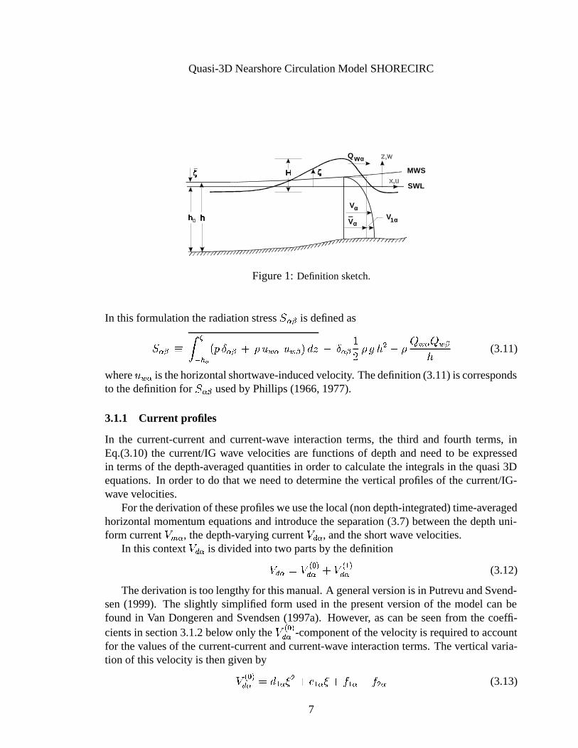
Fig 1 shows thedefinitionsof thecoordinatesystemandcomponentsof velocitiesusedin thefollowing. Thus
�#representsthemeansurfaceelevation and $�% is thestill waterdepth.
Thelocalwaterdepthi thendeterminedas$ � $�& � # (3.2)' � representsthetotal volumeflux which is definedby
' �(� )+*,.-0/ ���213� (3.3)
and' ��� is thevolumeflux dueto theshortwavemotion definedby
5
Quasi-3DNearshoreCirculationModelSHORECIRC
' ���4� ) *,.-5/ ��� �61.�7� ) **98 ��� �61.� (3.4)
where#5:
is theelevationof thewave trough.Hencewe have ' �;� )=<*,.- / � �213� � ' ��� (3.5)
The currentvelocity � � is divided into a depthuniform part ��> � anda depth-varyingpart ��? � by � �;� ��> � ����? � (3.6)
where ��> � is definedby ��> �;� ' �A@ ' � �$�% � �# (3.7)
This impliesthat ) <*-0/ ��? �213�4�B (3.8)
Thecurrent � � is thecurrentthatwould bemeasuredby a currentmeterplacedbelowtroughlevel. Noticethat thedefinitionsof ��> � and ��? � differ slightly from thedefinitionsof C� � and ��D � usedin Putrevu andSvendsenandin someof theearlierpublicationson themodel.Thisonly influencestheform of thedispersivemixing coefficientsdescribedbelow,but hasbeenfoundto havea favorableinfluenceon therobustnessof themodel.
In theequationsbelow E �GF is theReynoldsstress,while E�HF and E�IF representthesurfaceandthebottomshearstress,respectively.
The SHORECIRCmodel is basedon the depth-integrated, time-averagedequationswhich in completeform andin tensornotationread:J �#J � � J ' �J ��� �K (3.9)
J ' FJ � � JJ ���+L ' � ' F$ M � JJ ��� ) <*,.-ON ��? � ��? FP1.� � JJ ��� ) ** 8 ��� � ��? F � ��� F ��? �213�� Q � $�& � �# � J �#J ��F @ E HFR � E IFR � SR JJ ���UTWV �GFX@ ) *,.- N E �GF213�ZY[�\ (3.10)
6
Quasi-3DNearshoreCirculationModelSHORECIRC
VααV1αα
Vαα
Q ααw
SWL
MWS
Figure1: Definition sketch.
In this formulation theradiationstressV �GF is definedas
V �GF7] ) *,.- / �_^�`O�GF � Ra��� �b��� FZ��13�c@d`O�GF Se R Q $�f @4R ' ��� ' �gF$ (3.11)
where��� � is thehorizontalshortwave-inducedvelocity. Thedefinition(3.11)iscorrespondsto thedefinitionfor V �GF usedby Phillips (1966,1977).
3.1.1 Curr ent profiles
In the current-currentand current-wave interactionterms, the third and fourth terms, inEq.(3.10)the current/IGwave velocitiesare functionsof depthandneedto be expressedin termsof thedepth-averagedquantities in orderto calculatethe integralsin thequasi3Dequations.In orderto do thatwe needto determinetheverticalprofilesof thecurrent/IG-wavevelocities.
For thederivation of theseprofilesweusethelocal(nondepth-integrated)time-averagedhorizontalmomentum equationsandintroducetheseparation(3.7) betweenthedepthuni-form current ��> � , thedepth-varyingcurrent �h? � , andtheshortwavevelocities.
In thiscontext �h? � is dividedinto two partsby thedefinition��? ��� �ji &lk? � ���ji D k? � (3.12)
Thederivation is toolengthyfor thismanual.A generalversionis in Putrevu andSvend-sen(1999). The slightly simplified form usedin the presentversionof the modelcanbefound in Van DongerenandSvendsen(1997a). However, ascanbe seenfrom the coeffi-cientsin section3.1.2below only the �mi &lk? � -componentof thevelocity is requiredto accountfor thevaluesof thecurrent-currentandcurrent-wave interactionterms.Theverticalvaria-tion of thisvelocity is thengiven by��i &lk? � �\1 D �on f �qpoD �rn �qstD � ��s f � (3.13)
7
Quasi-3DNearshoreCirculationModelSHORECIRC
where nA�\� � $�& (3.14)
and 1 D � � @vu �erw : (3.15)poD � � E�I�R w : (3.16)srD � � @ $ e E�I�Rh� w : � (3.17)s f � � $ f u �x � w : � (3.18)
(3.19)
with u � givenby
u �;�dy SR $ J V ��GFJ ��F � E I�R $ @ s ��z|{ (3.20)
where s �j� JJ ��� � ��� �Z��� FZ� � JJ � � ��� �r}~���O{ (3.21)
In addition, � i D k? � is givenby� i D k? � � � i D�� � k? � �q� i D�� � k? � ��� i D�� � k? � ��� i D�� � k? � (3.22)
with ��i D�� � k? � � ��i D�� �0� � k? � n � ����i D�� �0� � k? � n � �q��i D�� �5� f k? � n f (3.23)� i D�� � k? � � � i D�� ��� � k? � n � ��� i D�� ��� � k? � n � ��� i D�� ��� f k? � n f (3.24)� i D�� � k? � � � i D�� � � � k? � n � ��� i D�� � � � k? � n � �q� i D�� � � f k? � n f (3.25)
and � i D�� � k? � � � � i D�� �0� � k? � ��� i D�� ��� � k? � �q� i D�� � � � k? � � $ ��� � i D�� �0� � k? � ��� i D�� ��� � k? � �q� i D�� � � � k? � � $ ��� �ji D�� �0� f k? � ���ji D�� ��� f k? � �q�ji D�� � � f k? � � $ f� { (3.26)
Furtherdetailsabout ��i D k? � canbefoundin HaasandSvendsen(2000).
8
Quasi-3DNearshoreCirculationModelSHORECIRC
3.1.2 Dispersivemixing coefficients(3-D version)
Fromthecurrent/IG-wavevelocityprofilesthecurrent-currentandcurrent-wave interactiontermsin (3.10)canberewritten in termsof a setof coefficients � �GF , � ��� , � �GF , and � �GFO�which are the 3D dispersioncoefficients. As shown by SvendsenandPutrevu (1994)thedispersive mixing representedby thesecoefficientscanaccountfor a majorpartof the lat-eralmixing in thenearshoreregion. Thesecoefficientscanall becalculatedfrom thedepthvaryingpart ��? � of thecurrentvelocity profiles. Thegeneraldefinitionsof thecoefficientsaregiven in Putrevu andSvendsen(1999).Theversionusedherecorrespondsto themodi-fiedversionversionusedby HaasandSvendsen(2000a)whichdiffersin thewaythecurrentvelocity is split in meananddepthvaryingpartsasshown in (3.6).The3D-dispersioncoef-ficientsaredefinedby
� �GF�� � @�� ) *,.- / S� w : ��T )q�,.- / J � i &lk? �J ��� @ J6���G�-J ��� @ J $�%J ��� J � i &lk? �J � Y L )��,.- / ��i &lk? F @ ' � F$ 13� � M 13�� ) *,.-0/ S� w : ��T ) �,.-0/ J � i &lk? FJ ��� @ J � �G�-J ��� @ J $�%J ��� J � i &lk? FJ � Y L ) �,.-0/ � i &lk? � @ ' ���$ 13� � M 1.���(3.27)� �GF ��@ S$ � ) *,.-0/ S� w : ��T ) �,.-0/ � $�% � � � � J � i &lk? �J � 13� � Y L ) �,.-0/ � i &lk? F @ ' �gF$ 13� � M 1.� �) *,.- / S� w : ��T ) �,.- / � $�% � � � � J � i &lk? FJ � 13� � Y L ) �,.- / � i &lk? � @ ' ���$ 1.� � M 13��� (3.28)
� �GF � S$ ) *,.- / S� w : � L )��,.- / �ji &lk? � @ ' ���$ 1.� � M L )��,.- / ��i &lk? F @ ' � F$ 1.� � M 13� (3.29)
� �GF � ) *,.- / � i &lk? � � i &lk? F 1.� �q� i &lk? F � # � ' � � ��� i &lk? � � # � ' � F (3.30)
The valuesof the 3D-dispersion coefficients implementedin the presentform of theSHORECIRChavebeendeterminedfor thesimplifiedcaseof adepthuniformeddyviscos-ity
w :andquasisteadyflow. 1
In theprogramthereareoptionsto usethe3-D dispersionor to do computations in the2-D horizontalmodewith depthuniform currents.Operationwith depthuniform currentsimpliesthatthedispersivemixing is turnedoff. Theonly lateralmixing is thenprovidedbyw :
in (3.49). This will usuallyprovide too litt le lateralmixing. Dependingon theproblemunderstudythevaluesof
w :in (3.49)mayhave to be increasedsubstantially (typically by
1It is emphasizedherethat although theseformulas only contain �� ¢¡¤£¥�¦ the full effect of �§ ©¨9£¥�¦ in (3.12) isincluded becausein the above expressionsfor thedispersive mixing coefficientsthecontributions involving� ©¨9£¥�¦ havebeenexpressedanalytically in termsof � ¢¡¤£¥�¦ . SeePutrevu andSvendsen(1999),Appendix B.
9
Quasi-3DNearshoreCirculationModelSHORECIRC
a factorof 10 - 20) to compensatefor themissing 3-D mixing. For further discussion seesection3.3.2.
3.1.3 Final form of the basicequations
Using thesecoefficientstheequationscanthenbe written in termsof surfaceelevations#
andthetotal volumeflux components'�ª
and'¬«
asdependentunknowns. TheresultisJ #J � � J '¬ªJ � � J '¬«J �\ (3.31)
and J 'ªJ � � JJ � � ' fª$ � � ª0ª � � JJ � 'ª®'¬«$ � � ª0« �@ JJ � $°¯ � e � ª0ª � � ª0ª � JJ � � '¬ª$ � � e � ª0« JJ � '¬ª$ � � � ª0ª JJ � '«$ �l±@ JJ $�¯ � � ª0« � � ª0« � JJ � � 'ª$ � � � «�« JJ � 'ª$ � � � ª0ª JJ � � '¬«$ � � � � ª0« � � ª0« � JJ � '«$ �l±� JJ � ¯²� ª0ª0ª 'ª$ � � ª0ª0« '«$ ± � JJ ¯²� ª0«³ª 'ª$ � � ª0«�« '¬«$ ±��@ Q $ J �#J � @ SR � J V ª0ªJ � � J V ª0«J � � SR � JJ � ) *,.-5N E ª0ª 13� � JJ ) *,.-ON E ª0« 1.�r�� E�Hª @ E�IªR (3.32)
J '¬«J � � JJ � � '¬ª®'¬«$ � � ª0« � � JJ � ' f«$ � � «³« �@ JJ � $°¯ � � ª0« � � ª0« � JJ � � '¬ª$ � � � «³« JJ � '¬ª$ � � � ª0ª JJ � � '¬«$ � � � � ª0« � � ª0« � JJ � '¬«$ �l±@ JJ $°¯´� «³« JJ � � '¬ª$ � � e � ª0« JJ � � '¬«$ � � � e � «³« � � «�« � JJ � '¬«$ �l±� JJ � ¯²� ª0«³ª 'ª$ � � ª0«³« '¬«$ ± � JJ ¯²� «³«³ª 'ª$ � � «³«�« '«$ ±�µ@ Q $ J �#J @ SR � J V ª0«J � � J V «³«J � � SR � JJ � ) *,.-5N E ª0« 13� � JJ ) *,.-ON E «³« 13�t�� E�H« @ E�I«R (3.33)
In theabove, E�I� � E � , arethebottomshearstresses,thesurface(wind) shearstresses,andV �GFg� E �GF aretheradiationstressesandtheturbulentReynold’sstresses,respectively.
10
Quasi-3DNearshoreCirculationModelSHORECIRC
The equations(3.31), (3.32)and(3.33)arethe equationssolved by the SHORECIRCmodel.
As mentionedthevaluesofw :
and E IF usedin themodelarespecifiedin sections3.5and3.3,respectively.
3.2 Short wavequantities
3.2.1 The wavedri ver
Theshortwavedriverdeterminestheshortwavemotionandcalculatestheshortaveragedforcing thatdrivesthecurrentsandIG waves.Therearetwo optionsfor modelingtheshortwaves: usingthe built in wave driver, or usinga separatewave driver andspecifyingthewave inputvia datafiles. Additional informationaboutwhatdatafiles to includeis giveninsection5.4
In thepresentversionof theSHORECIRCmodel,animprovedversionof theREF/DIF1(Kirby andDalrymple,1994)is incorporatedastheshortwavedriver. TheREF/DIFpackageis includedasa subroutinewithin the code. However, it only provides the wave heights,wave angles,wave celeritiesand group velocities. The associatedshort wave forcing iscalculatedin aseparatesubroutine¶0·�¸º¹5»9¼2½Z¾Z¿ ÀZ¹5Á�¾Z¿O¹ whichalsocallstheREF/DIF.
The REF/DIF wave driver is basedon the parabolicapproximationof the mild-slopeequation,andaccountsfor refraction, diffraction,shoalingandbreakingphenomena.Thepresentversionusesa single offshorewave heightanddirection,althoughit canrepresentthepeakin aspectrum.
Wave/currentinteractionis importantfor many applicationswith strongcurrentssuchasrip currents.It is modelledby periodicallyrecalculatingthewave forcing including theef-fectsof currentsandsetup.Theintervalsbetweeneachrecalculationof thewaveconditionscanbechosenin theinput for thecalculation.
Thewave-currentinteractionis includedasanoptionin thecodewhenthebuild-in wavedriver is used.Whenusingaseparatewavedriver via thedatafileswave-currentinteractionis only possible by doing a hot startwith the newly calculatedwaveseachtime the waveconditionshavebeenupdated.
3.2.2 The short wave forcing
As mentionedtheshortwaveforcingrepresentsthetime-averagedcontributionsto themassandmomentumequationsgeneratedby theshortwave motion. Thesecontributionsaretheshortwavemassflux
' ��� andtheradiationstressesV �GF .Radiation StressUsingthe resultsof wave heightsandwave anglescalculatedby theshort-wave-driver theradiationstressesarecalculated.Thegeneralizedradiationstressestensoris givenbyV �GFA� p �GF V >� `O�GF V à (3.34)
11
Quasi-3DNearshoreCirculationModelSHORECIRC
where p �GFA�ÅÄ�Æ�ÇrÈ f ! � È�ÉËÊ ! � Æ�ÇZÈ ! �È�ÉËÊ ! � Æ�ÇrÈ ! � È�ÉËÊ f ! � Ì (3.35)
and ! � is thewave anglerelative to thepositive � axis. ThescalarsV > and V Ã aredefinedas
V > � ) *,.-5N Rt��� f 13� (3.36)
V Ã � @Í) *,.-5N Rt}~� f 13� �dSe R Q Î f (3.37)
where ���|�mÏ®��� �ÐÏ (3.38)
is thewaveparticlevelocity in thewavedirection.In thecalculationof V �GF themodelusesthelocal waveheightsdeterminedby thewave
driver(presentlyREF/DIF1).Outsidethesurfzonetheresultsfor sinusoidalwavesareused.For sinusoidalwaveswehave V > � SS x R QjÑ f � S �+Ò � (3.39)V Ã � SS x R QjÑ f Ò (3.40)
where Ò is Ò � erÓ $È�ÉËÊ Ô eZÓ $ (3.41)
Inside the surfzonethoseresultsare augmentedwith the contribution from the rollerusingtheresultsfrom Svendsen(1984).Thus V > and V Ã aredeterminedas
V > �KR QgÑ f°Õ fQ $ ¯´��& � �ÑvÖ $Ñ ±��KR Q Ñ f×Õ fQ $ ¯¢��& � �Ñ f $Ö ± (3.42)
and V à � Se R QgÑ f0��& (3.43)
where� is theroller areaand �§& is thewaveshapeparameterdefinedby��& � SØ )+Ù& � ÎÑ � f 1r� (3.44)
Thus V �GF is computedas
V �GFA� p �GFZR Q Ñ f Õ fQ $ ¯¢�§& � �Ñ f $Ö ± � `O�GF Se R QgÑ f��& (3.45)
12
Quasi-3DNearshoreCirculationModelSHORECIRC
A transition is establishedbetweenthe two expressionsfor V �GF to simulatethegrowthof theroller whenbreakingstarts.
Parameterizationsfor ��& canbefoundin Hansen(1990).For sinusoidal longwavesthevalueof ��& is
DÚ . In thepresentversionof themodelthis is usedasthedefault value.Noticethat Ö is calculatedas Õ Ø whereÕ is thelocal valueof thephasevelocity.
WaveVolumeFluxOutside thesurf zone,thewavevolumeflux is givenby' � �;� ��& QgÑ fÕ Ó �Ó (3.46)
whereÓ � is the wave numbervector in direction ��� , Ó �Û� Ó � Õ�ÜoÝ ! �°� ÝGÞ�ß ! ��� andc is the
valueof thephasevelocity.Insidethesurf zone,thewavevolumeflux is givenby (Svendsen1984)' ���;� QgÑ fÕ Õ fQ $ � ��& � �ÑvÖ $Ñ � Ó �Ó � QgÑ fÕ Õ fQ $ � ��& � �Ñ f $Ö � Ó �Ó (3.47)
As for the radiationstressa transition is establishedbetweenthe two expressionsfor' ��� to simulatethegrowth of theroller whenbreakingstarts.In theexpressions for boththeradiationstressandthevolumeflux theroller area� may
be approximatedby either {áà Ñ f (Svendsen,1984)or by {á x ÑvÖ (Okayasuet al., 1986).Thelatteris usedasdefault in thepresentversionof theprogram.
3.3 Turbulencemodelling
3.3.1 The quasi-3Dversion
In thequasi-3Dversionof themodeltheturbulentshearstressesarecalculatedby theeddyviscosity model,as E �GF;�KR w : � J ��> �J ��F � J ��> FJ ��� � (3.48)
(3.48)is depthuniform. However, sincethecontribution from E �GF is generallysmall this itis a reasonableapproximation.
Theeddyviscosity formulation accountsfor bothwave-breakingandbottomgeneratedturbulence.Outsidethesurf zone,themodelis basedon SvendsenandPutrevu (1994)andCoffey andNielsen(1984).Insidethesurfzone,amodifiedBattjes(1975)modelis applied.Thecombinedcontributionsto theeddyviscosity from thesesourcesis calculatedasw : �ãâ D³äæå s �e � &0$ � �ã$ � � R � Dèç¤� � w : � & � woé (3.49)
whereä is thevonKarmanconstant( ämê { � ), s � is thewaverelatedbottomfriction coeffi-cient(sect3.5). � & is theshort-waveparticlevelocity amplitudeevaluatedat thebottom, and
13
Quasi-3DNearshoreCirculationModelSHORECIRC
� is theenergy dissipation per unit areagiven by the formulationusedin theREFë DIF1.Thefirst termin equation(3.49)representsthebottominducedturbulencewhich is alwayspresentandthesecondtermrepresentsthewavebreakinginducedturbulencewhich is onlypresentin thesurf zone.By comparingtheeddyviscosity estimatesfrom thisequationwiththeexperimentalresultsof NadaokaandKondoh(1982) andthevaluessuggestedby Svend-sen(1987),â D~ê { e . For � valuesbetween0.05wnd 0.1arerecommended.As a defaultthevalue � �= {á rì shouldbeused.Theconstant
w : � & is anempiricalmeasureof theback-groundeddyviscosity foundoffshore.
ThesubgridstressesaremodelledbyusingtheSmagorinsky eddyviscositymodel(Smagorin-sky 1963). TheSmagorinsky eddyviscosity modelsthe turbulencegeneratedby theshearin theflow andaccountsfor thedissipationby theeddieswhicharetoosmallto beresolvedby thegrid resolution.
Thefollowingequationis usedto calculatetheSmagorinksyeddyviscositywoé ���èâ é³í � foî e p �GF p �GF (3.50)
where í � î í � í (3.51)ï �GFA� Se L J�ð > �J ��F � J�ð > FJ ��� M (3.52)â é is theSmagorinksycoefficientandhasa typicalvalueof {á ��ñ â éòñ g{ er� .While
w :is of relatively limiteddirect importancethrough(3.48)themajor functionofw :
is throughits influenceon theverticalcurrentprofilesandtherebytheexpressionsfor thedispersive lateralmixingcoefficientsgivenby (3.27),(3.28),(3.29),and(3.30).
3.3.2 The 2-D model version
If the quasi-3Doption is turnedoff the modelwill operateasa 2-D model. The 2-Dversionof themodelis enhancedrelative to traditional2-D modelsbecauseof theinclusionof
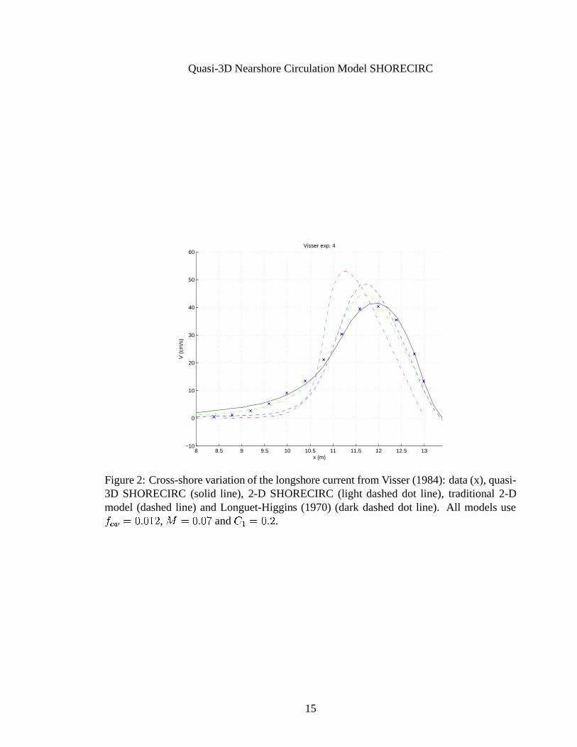
���G�º� �G�- in the modified radiationstressgiven by 3.11. This extra term enhancesthelateralmixing of atraditional2-D model.Figure(2) demonstratestheeffectof thequasi-3Dmixing, theenhanced2-D containedin SHORECIRC, thetraditional2-D andtheLonguet-Higgins(1970)analyticalsolution(hereafterreferredto asL-H) by showing thecross-shorevariationof thelongshorecurrentfrom thelaboratoryexperimentby Visser(1984).Clearlythequasi-3Dversionfits thedatathebest.The2-D versionshave largepeaksaswell asthewrong shapefor the cross-shoreprofile of the longshorecurrent. However, the additionalmixing containedby the2-D SHORECIRCis evidentby thechangein thepeakandwidthof thecross-shoreprofileof thelongshorecurrentrelativeto thetraditional 2-D version.ThedifferencebetweentheL-H andtraditional2-D is dueto thesimple wave forcing basedonasaturatedbreaker utilizedby L-H.
For mostpracticalapplications,whenonly usingthe2-D versionof themodel,theeddyviscosity needsto beenhancedsubstantially to compensatefor themissing dispersive mix-ing in orderto give reasonableresults.In doingso it shouldbe rememberedthat in nature
14
Quasi-3DNearshoreCirculationModelSHORECIRC
8 8.5 9 9.5 10 10.5 11 11.5 12 12.5 13−10
0
10
20
30
40
50
60
x (m)
V (
cm/s
)
Visser exp. 4
Figure2: Cross-shorevariationof thelongshorecurrentfrom Visser(1984):data(x), quasi-3D SHORECIRC(solid line), 2-D SHORECIRC(light dasheddot line), traditional 2-Dmodel(dashedline) andLonguet-Higgins (1970) (dark dasheddot line). All modelsuses®� �ó�\ {á S e , � �K {ô rõ and â D �ã { e .
15
Quasi-3DNearshoreCirculationModelSHORECIRC
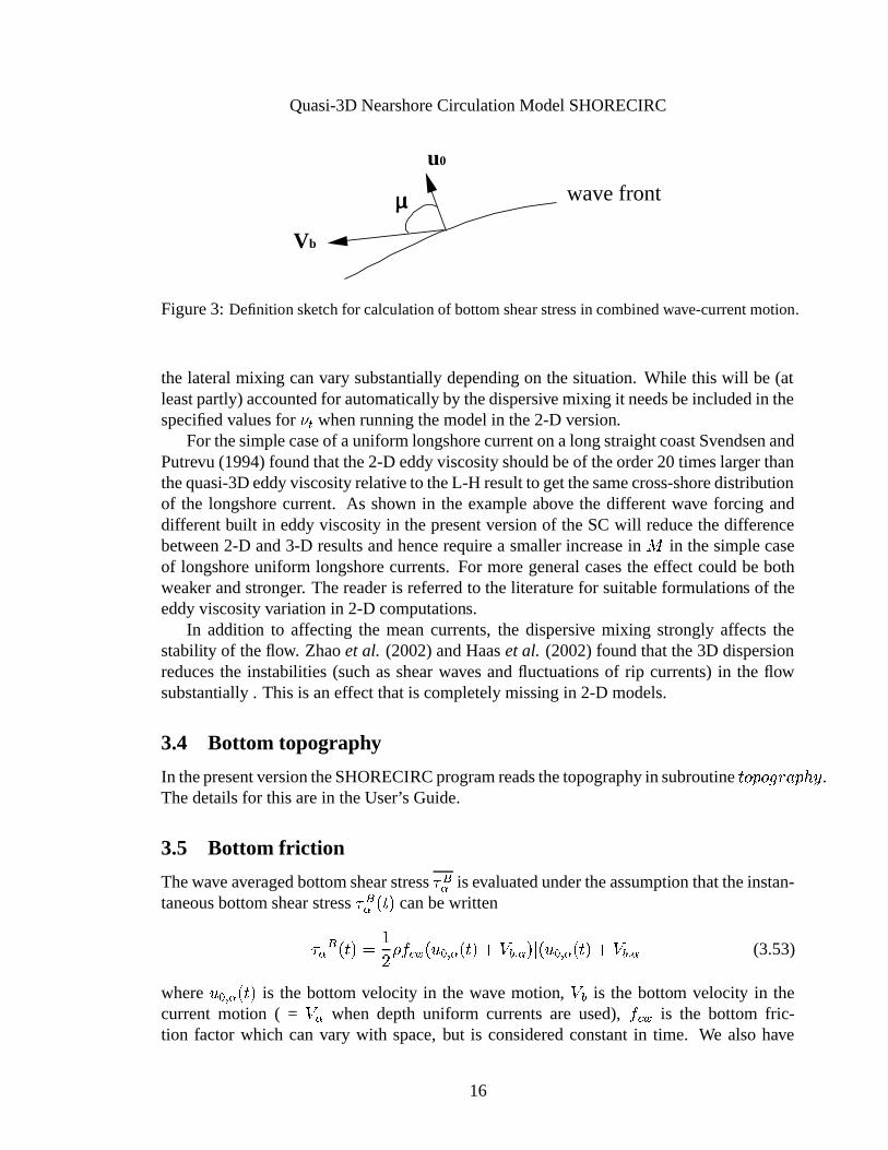
µ
Vb
u0
wave front
Figure3: Definition sketch for calculation of bottomshear stressin combinedwave-currentmotion.
the lateralmixing canvary substantially dependingon thesituation. While this will be (atleastpartly)accountedfor automaticallyby thedispersivemixing it needsbeincludedin thespecifiedvaluesfor
w :whenrunningthemodelin the2-D version.
For thesimplecaseof auniformlongshorecurrentonalongstraightcoastSvendsenandPutrevu (1994)foundthatthe2-D eddyviscosityshouldbeof theorder20timeslargerthanthequasi-3Deddyviscosityrelativeto theL-H resultto getthesamecross-shoredistributionof the longshore current. As shown in the exampleabove the differentwave forcing anddifferentbuilt in eddyviscosityin thepresentversionof theSC will reducethedifferencebetween2-D and3-D resultsandhencerequirea smallerincreasein � in thesimplecaseof longshoreuniform longshorecurrents.For moregeneralcasestheeffect could bebothweaker andstronger. Thereaderis referredto theliteraturefor suitableformulations of theeddyviscosityvariation in 2-D computations.
In addition to affecting the meancurrents,the dispersive mixing stronglyaffects thestability of theflow. Zhaoet al. (2002)andHaaset al. (2002)foundthatthe3D dispersionreducesthe instabilities (suchasshearwavesandfluctuationsof rip currents)in the flowsubstantially . This is aneffect thatis completelymissing in 2-D models.
3.4 Bottom topography
In thepresentversiontheSHORECIRCprogramreadsthetopographyin subroutine� Ü ^ Ü Qgöo÷ ^ $ .Thedetailsfor thisarein theUser’s Guide.
3.5 Bottom friction
ThewaveaveragedbottomshearstressE I� is evaluatedundertheassumptionthattheinstan-taneousbottomshearstressE I� �ø��� canbewrittenE � I �����2� Se R sº� �æ�9� & � ������� ������� �.�®Ï_�9� & � ������� ������� ��Ï (3.53)
where � & � ���ø��� is the bottomvelocity in the wave motion, ��� is the bottom velocity in thecurrent motion ( = � � when depth uniform currentsare used), sZ� � is the bottom fric-tion factorwhich canvary with space,but is consideredconstantin time. We alsohave
16
Quasi-3DNearshoreCirculationModelSHORECIRC� & �;�[�9� & ª ��� & « � , ��� �;�[� ��� ª � ��� « � .After shortwaveaveragingthisexpressionfor E I� canbewritten(SvendsenandPutrevu,
1990), E I� � Se R sº� ��� & � " D���� � � " f � & �3�5{ (3.54)
For sinusoidalwaves,with Ϻ� & � �ÐÏ´��� & ÕOÜZÝúù (3.55)
with ù the phaseanglein the wave motion, the weight factorsfor the currentand wavemotion " D and " f are,respectively.
" D � ¯ � ���� & � f � e ���� & Æ�ÇrÈ ù Æ�ÇrÈ�û � Æ�ÇZÈ f ù ± Dèç f (3.56)" f � Æ�ÇrÈ ù ¯ � ���� & � f � e ���� & Æ�ÇrÈ ù Æ�ÇrÈ�û � Æ�ÇZÈ f ù ± Dèç f (3.57)
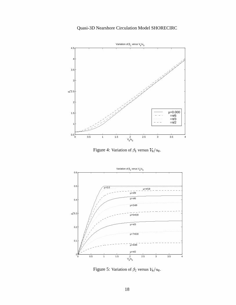
In theaboveequations,ù is theshort-wavephaseangle,ù ��ü6� @ÍýÂþÓ ÿ 1 þ� , and û is theanglebetweentheshort-wavedirectionandthecurrentvelocityat thebottom. For definitionsseefigure3. Wehavealsodefined ��� � Ï ����� ��Ï (3.58)
Thecorrespondingvariationsof " D and " f versus��� ë � & and û areshown in figure4 andfigure5.
In thecodethevaluesof " D and " f areapproximatedby simple curve fits to (3.57)and(3.57).
Steady-streamingIt hasbeenfound (seePutrevu andSvendsen,1995) that particularlyoutside the surf
zonethesteadystreaminginducedin theoscillatory bottomboundarylayeris importantforthepropermodellingof theundertow. In themomentumequationthis is representedby the���h}~� -stresswhich is modelledhereby theexpression foundby Longuet-Higgins,(1956).
3.6 Boundary conditions
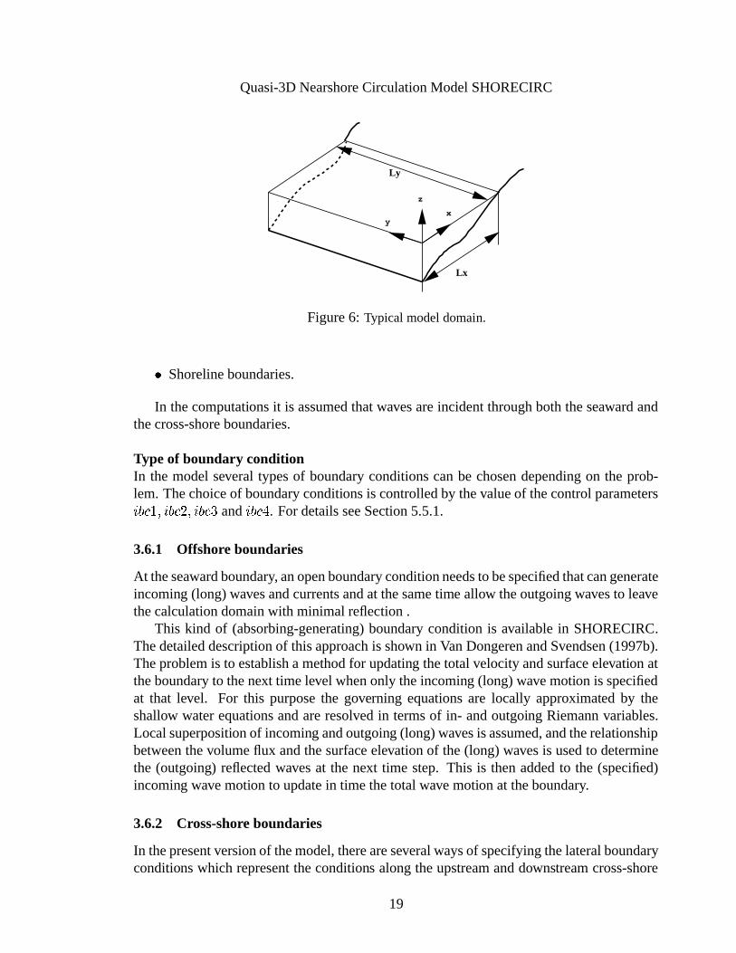
Theequationsaretypically solvedin a rectangulardomainof thecoastalregion. SeeFig. 6for a sketchof a typicalmodeldomain.Boundaryconditionsthereforeneedto bespecifiedalongthreedifferenttypesof boundaries:
� Seawardboundaries.
� Cross-shoreboundaries.
17
Quasi-3DNearshoreCirculationModelSHORECIRC
0 0.5 1 1.5 2 2.5 3 3.5 40.5
1
1.5
2
2.5
3
3.5
4
4.5
Variation of β1 verus V
b/u
0
Vb/u
0
β 1
µ=0.000 =π/6 =π/3 =π/2
Figure4: Variation of� D versus � ����� & .
0 0.5 1 1.5 2 2.5 3 3.5 40
0.1
0.2
0.3
0.4
0.5
0.6
µ=0.0 µ=π/18
µ=π/9
µ=π/6
µ=2π/9
µ=5π/18
µ=π/3
µ=7π/18
µ=4π/9
µ=π/2
Variation of β2 verus V
b/u
0
Vb/u
0
β 2
Figure5: Variation of� f versus � ����� & .
18
Quasi-3DNearshoreCirculationModelSHORECIRC
y
z
x
Lx
Ly
Figure6: Typical modeldomain.
� Shorelineboundaries.
In thecomputationsit is assumedthatwavesareincidentthroughboththeseawardandthecross-shoreboundaries.
Typeof boundary conditionIn the modelseveral typesof boundaryconditionscanbe chosendependingon the prob-lem. Thechoiceof boundaryconditionsis controlledby thevalueof thecontrolparametersÞ � Õ S � Þ � Õ e � Þ � Õ � and Þ � Õ � . For detailsseeSection5.5.1.
3.6.1 Offshoreboundaries
At theseawardboundary, anopenboundaryconditionneedsto bespecifiedthatcangenerateincoming (long)wavesandcurrentsandat thesametimeallow theoutgoingwavesto leavethecalculationdomainwith minimal reflection .
This kind of (absorbing-generating)boundarycondition is available in SHORECIRC.Thedetaileddescriptionof thisapproachis shown in VanDongerenandSvendsen(1997b).Theproblemis to establishamethodfor updating thetotal velocityandsurfaceelevationattheboundaryto thenext time level whenonly theincoming (long)wavemotion is specifiedat that level. For this purposethe governing equationsare locally approximated by theshallow waterequationsandareresolved in termsof in- andoutgoing Riemannvariables.Localsuperpositionof incoming andoutgoing (long)wavesis assumed,andtherelationshipbetweenthevolumeflux andthesurfaceelevationof the(long) wavesis usedto determinethe (outgoing) reflectedwavesat the next time step. This is thenaddedto the (specified)incoming wavemotion to updatein time thetotalwavemotionat theboundary.
3.6.2 Cross-shoreboundaries
In thepresentversionof themodel,thereareseveralwaysof specifyingthelateralboundaryconditionswhich representtheconditions alongtheupstreamanddownstreamcross-shore
19
Quasi-3DNearshoreCirculationModelSHORECIRC
boundaries(in the senseof the dominatinglongshorecurrent). The following optionsareavailable:
� A flux boundaryconditioncanbespecified. Thevolumeflux'�«
will thenneedto beprescribedatall pointsof thecross-shoreboundary.
� A wall alongtheboundarycanbeprescribed.In this caseboth';«
and * « areauto-maticallysetto zeroalongthecross-shoreboundary.
� A periodicboundaryconditioncanbeused.Thismeansthattheinstantaneousflow ateachpoint of oneof thecross-shoreboundariesis mirroredat theequivalent point oftheothercross-shoreboundary.
Noticethattheperiodicityconditiononly makessenseona coastwherethecross-shoreprofile is thesameat thetwo cross-shoreboundaries.
3.6.3 Shoreline boundary
Therearepresentlytwo optionsfor modeling theshoreline.Oneoptionis to usea no-fluxcondition which follows thestill watershorelineposition. Theboundarylocationis deter-minedwithin theprogrambasedon theinitial conditionsandis thenheldfixedthroughouttheentirecomputation. Both thecross-shoreandlongshorevolumefluxesaresetto zeroattheshoreline.
The otheroption is to placea vertical wall at a very small depth(a few cm) alongtheshoreline.Only thecross-shorevolumeflux is setto zero,no constraintis requiredon
'�«andin generalthe modelcomputes
';«�� alongthe shoreline.Analysisshows that thisusuallydoesnot influencethe circulationpatternnoticeably. However, the option of anartificial shelfat theshorelineis not recommendedbecausethis maydisturb thenearshoreflow significantly.
3.7 Wind surfacestress
Thewind-inducedsurfacestressis computedas(ChurchandThornton1993,Smithet al.,1993) E H� �Kâ �æRt��Ï�� Ï��Í� (3.59)
where � is the dragcoefficient, R3� is the air densityand � is the wind velocity at thestandard10melevation. Thewind dragcoefficient � is calculatedfrom the formula rec-ommendedby theWAMDI group(1988):
â � ê�� S { e ìtõ ��� S , � ð ñ õg{ ��� ë Ý�è g{ôì � g{ô xr� ð � � S , � ð�� õg{ ��� ë Ý (3.60)
20
Quasi-3DNearshoreCirculationModelSHORECIRC
3.8 Numerical solution scheme
Thesystemof governing equations(3.31)(3.32)(3.33)aresolvedusingPredictor-Correctorschemeoriginally developedfor Boussinesqequationsby Wei andKirby (1995). This isa centralfinite differenceschemeon a fixed spatialgrid which is implementedwith anexplicit third-orderAdams-Bashforthpredictoranda third-orderAdams-Moultoncorrectortime-stepping scheme.In spacethedifferenceschemeis fourthorderin thegrid size,exceptfor diffusion terms(termswith E �GF andthe3-D dispersive mixing terms)which aresecondorderin space.For detailsseeSanchoandSvendsen,(1997). In orderto solve thesystem,Eqs.(3.31)(3.32) and(3.33)arerewritten sothatonly the local accelerationappearson theleft-handside J��J � ��� (3.61)
where�
is thevectorquantitygivenby� � ¯ �# � '¬ª � '¬« ± Ù , and � is thevectorcorresponding
to theright handsideof thecontinuityandmomentumequations(3.31),(3.32),and(3.33).
In thepredictorstep,Eqs.(3.61) areapproximatedby theAdams-Bashforthscheme
��� � ! � ��" � ! �$#&% !(' � !*) � " � ! � !,+ � " , ) � ! � !(- � " , + � ! � �/. � #&% - � (3.62)
where !�& � S ë S e ! D � eZ� ! f ��@ S x ! � � �(3.63)
At thecorrectorstep,theAdams-Bashforth-Moultonmethodreads
��"10 ) � ! � ��" � ! �2#3% "4' �65 ) � � � ! � 5 + � " � ! � "4- � " , ) � ! � �/. � #&% - � (3.64)
and "�& � S ë S e ÷ D � � ÷ f �Kì " � ��@ S (3.65)
The grid sizesin the � and -directions (í ��� í respectively) canbe differentbut are
assumedto beconstantover thecomputationalregion.
FiltersFiltering of thesolution is usedto avoid unrealhigh-frequency disturbancesto develop.
Thefilters implementedin thecodearehighorderfilters whichdonotcreatenoticeablenumericaldissipation.
4 CAPABILITIES AND LIMIT ATIO NSOF THE SHORE-CIRC
The circulation part
21
Quasi-3DNearshoreCirculationModelSHORECIRC
Thecirculationpartof theSHORECIRC solvesthedepthintegratedcontinuity andmo-mentumequations, therebyproviding informationaboutthe total depthintegratedvolumefluxes
'ª � '« andthesurfaceelevations#. The vertical variationof the currentvelocities
(in magnitudeanddirection)arecalculatedaswell in theprocessandtheeffectof thisvari-ation is accountedfor in the determination of the solutions for
'�ª � '« , and#
throughthedispersivemixingcoefficients.
Thederivationof theseequationshave requiredonly thefollowing assumptions:- it is assumedthat the pressurein the currentandinfragravity wave motion is hydro-
static.- it is assumedthat it is possibleto do averagingover a wave period, if neededasa
moving average.Theserestrictionsareverymild andthebasiccirculationequationssolvedcantherefore
in generalbeconsideredveryaccurate.Inaccuraciesaremainlyassociatedwith theway theindividual termsareapproximated.
The computations of the nearshorecirculation takes placein the time domainand itoftenshows that,evenwhentheforcing is constantor slowly varying,theflow patternscanbehighly unsteady(shearwaves,time-varying rip currentsareexamples).
Essentiallimitationson the modelaccuracy arelinked to the approximations usedfortheturbulentstresses:
- Theturbulenceis representedonly by arelatively simplemodel.As aconsequencetheeddyviscosity governingtheverticalprofilesin thewave averagedmotion is constantoverdepth.
- Thebottomfriction is only representedby a simple friction factormodel.- Theflow in thebottomboundarylayeris notresolved.(For furtherdescriptionsee3.5).
The wavedri ver
The computations of the nearshorecirculationis basedon the distribution of the shortwavegeneratedmassflux andradiationstresseswhicharedeterminedfrom thewavedriver.At presenttheREF/DIFF1 is usedaswavedriver. This is imposesthefollowing limitationson themodelsystem:
- Theshortwavemotionmusthaveonewell definedfrequency andawaveheightwhichis constantin time. However, thesequantitiescanbethepeakvaluesof aspectrum.
- Theshortwave motionis supposedto have a dominating direction(parabolicapprox-imation). However theparabolicmodelusedin REF/DIF1is a ”wide anglemodel” whichallowssubstantialvariationsof thewavedirectionover themodeldomain.
- Reflection of theshortwave motionfrom steepslopesandobstaclescannotberepre-sented(mild slopeassumption).
The numerical scheme
Thenumericalschemeis of high orderwhich allows relatively largegrid-spacings,and
22
Quasi-3DNearshoreCirculationModelSHORECIRC
it is normallyquiterobust.Thoughnumericalinstabilitiesmayoccur, they areusuallycon-nectedwith unrealistically strongvariations over the vertical for the velocity profiles. Apossible remedyis to increasetheeddyviscosity.
However, thepresentversionof themodelhasseveralnumericalconstraints:- It is basedon a rectangulargrid in thehorizontalplanein thedirectionof thechosen
coordinatedirections.- Thegrid sizeis constantin acoordinatedirection(but candiffer in thetwo directions).
Too largegrid sizescanlimit theresolutionneartheshoreline.theWork is ongoingto lift someof theserestrictions.
5 USERGUIDE
5.1 Intr oduction
This sectionwill give a brief overview of theSHORECIRCmodelstructureandintroducetheprocedurefor usingthemodel.Thecompiling instructions,input files anddatafiles areall explained.Also, theoperatinginstructionsandmodeloutputarepresented.
5.2 SHORECIRC revision history
5.2.1 Original versionof the model
Thiswastheversionusedin theanalysisof VanDongerenet al. (1994)� Simplified dispersivemixing
� Analytical forcing
� Absorbing/generatingboundarycondition.
� Numericalschemeof 7 � í � � � í � f �5.2.2 Major changesappearing in version1.1
Thiswastheversiondescribedin VanDongeren& Svendsen(1997a)� First versionwith quasi-3Deffectsincluded.
5.2.3 Major changesappearing in version1.2
Thiswastheversiondescribedin SanchoandSvendsen(1997)� Numericalschemeof 7 � í � � � í � � �� REF/DIFforcing
� Basisfor first standardizedversion
23
Quasi-3DNearshoreCirculationModelSHORECIRC
5.2.4 Major changesappearing in version1.3
This is the model versionusedtill the end of 2001 and describedin Van DongerenandSvendsen(2000).
� Upgradeof quasi-3Dtermsto form describedin thismanual
� Wave/currentinteractionincluded.
� Createdmoreuserfriendly environmentwith many optional features
5.2.5 Major changesappearing in version2.0
This is essentiallytheversiondescribedin HaasandSvendsen(2000a).
� Changeddefinitionof thedepthaveragedvelocity from C� to ��> and ��D to ��? .� Equivalentchangesin thedispersivemixing coefficients.
� Many additionalsmallimprovementsandbug-removals
� Addedno-fluxboundaryconditionfollowing thestill waterline
5.3 Overview of modeland flow chart.
TheShorecircpackageconsists of thewave andcirculationmodelaswell asprogramsforcreatingthetopographyandthe input controlfiles. Noticethat thewave driver includedisbasedon theREF/DIF. TheREF/DIFusedis basedon the theModified REF/DIF, Version2.5,whichhasbeenmodifiedfurtherto serveourneeds.
TheShorecircpackageis containedin thearchivefile sc20.tar,In orderto extractthefiles usethecommand
tar -xvf sc2_0.tar
Thiswill extract9 Fortranfiles,3 Fortran“include” files and1 compiling file.Seven of the Fortranfiles andthe three”include” files comprisethe programcodefor
themodel:
winc std main.f,winc std deriv.f,winc std time.f,winc std filter.f,winc std sub1.f,infile1.f,refdif2v25a.faswell asthreeincludedfiles
24
Quasi-3DNearshoreCirculationModelSHORECIRC
winc std common.incparam.h.pass.inc.
Oneof thetwo additional Fortranfiles is aprogramelement
createbath.f,
which is includedfor creatingcertainsimpletopographies.Runningthis file will interac-tively guidetheuserthroughthegeneration.Thisprogramelementcancreate
� aplanebeachof any slope,
� abeachwith aplateauin front
� or anequilibriumtypebeachwith aprofilegivenby � �98 .It canadda bar, by specifyingits height,width andposition, andplaceany numberof
channelsin thebar, specifyingtheirwidth andlocation.To input a measuredtopographyusersneedto createtheir own files. Note that the
topographydatamust provide information aboutthe water depthat all grid points. Theprogramwill readcolumns correspondingto ���h� $ values.
TheotherFortranfile,
createinput.f
is usedto createtheusercontrolledinput (otherthantopography)for operatingthemodel.Thecompilingfile
Makefile.
producesthecompilationoperationandlinking of theexecutable files.
The main program and its subroutines.
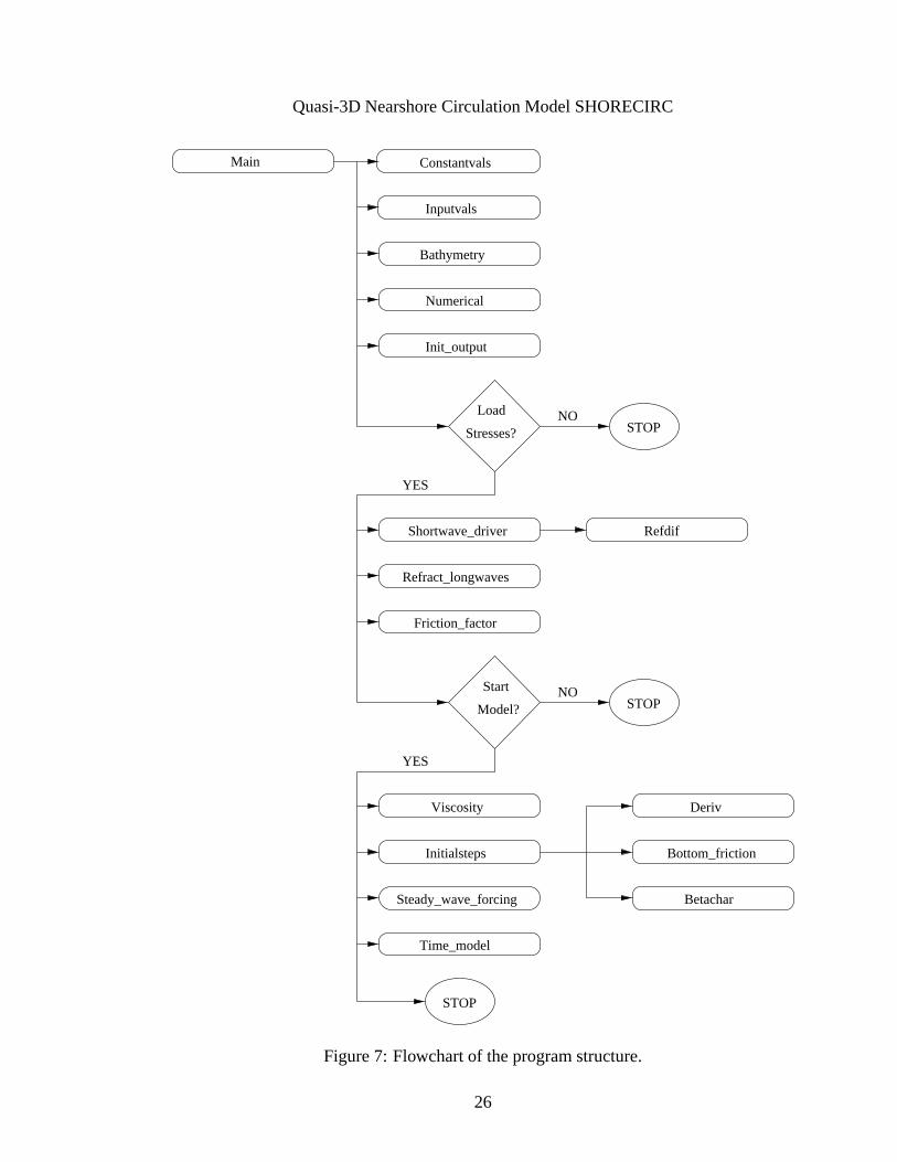
Thecentralelementof themodelis themainprogramcalledmain. Thefunctionof thispart is to call all therelevantsubroutines. Most of theseroutinesaswell asthemain itselfareall includedin the file calledwinc std main.f. Theseroutinesprimarily establishthebackgroundfor thecomputationandthuspreparesfor theintegrationin timethatconstitutesthemajorpartof a modelrun.
Thestructureof this partof theprogramis givenin Figure7. Theflowchartshows thesubroutinescalledby main in theorderthatthey arecalledaswell asany othersubroutinesthatarecalledby thesubroutines.
25
Quasi-3DNearshoreCirculationModelSHORECIRC
Load
Stresses?
Steady_wave_forcing
STOP
STOP
STOP
Numerical
Init_output
Shortwave_driver
Refract_longwaves
Friction_factor
Viscosity
Initialsteps
Time_model
Main Constantvals
Inputvals
Model?
Start
Deriv
Bottom_friction
Betachar
Bathymetry
NO
YES
NO
YES
Refdif
Figure7: Flowchartof theprogramstructure.
26
Quasi-3DNearshoreCirculationModelSHORECIRC
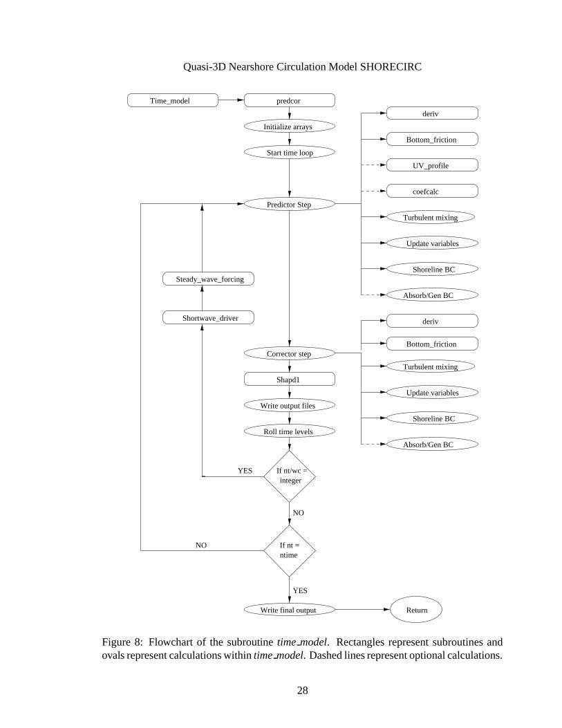
The last routinewhich is calledby main is the routine time model, locatedin the filewinc std time.f, which performsthe time integration. During this processis alsocalledaseriesof additionalsubroutines.Theseroutinesare containedin the otherprogramfileslistedabove. Thestructureof thesubroutinetime modelis shown in theflowchartFigure8.Theflowchartshows theorderin which thecalculationsareperformed.
Note that mostpertinentresultsarecalculatedduring the time integration. Thereforemostof the outputfiles aregeneratedduring the time computation within the time modelsubroutine.
List of program subroutinescalled fr om main.
Thefollowing is a list of thesubroutinescalledfrom main. It alsoidentifiesthefiles inwhich they arelocated.
� main. Themainprogramwhichcallsthefollowing routines.Containedinwinc std main.f.
� constantvals. This definesthe physical and mathematicalconstants.Containedinwinc std main.f.
� inputvals. Theinputfile is readfrom thissubroutine.Containedin winc std main.f.
� topography. Thisspecifiesthetopography, eitherfromafile oranalytically. Containedin winc std main.f.
� numerical. Thissetsup thenumericalparameters.Containedin winc std main.f.
� init output. This initializestheoutputfiles. Containedin winc std main.f.
� refract longwaves. Calculatestheangleof incidenceof longwavesenteringthecom-putationaldomainfrom outside.Containedin winc std main.f.
� shortwavedriver. This routinecalls theshortwave driver (REF/DIF)andcalculatestheshort-waveparameters.This includestheradiationstressV � � F andtheshortwaveinducedmassflux,
' � � . Containedin winc std main.f.
� friction factor. Thiscalculatesaspatiallyvaryingbottomfriction factor. It caneasilybesubstitutedby aconstantfriction factor. Containedin winc std main.f.
� viscosity. This evaluatesthe turbulent eddyviscosity coefficient,w :
. Containedinwinc std main.f.
� initialsteps. In this subroutine thearraysfor timesteps��� @ eZí �5�G@ í �5�0 arefilled.Containedin winc std main.f.
� waveforcing. The subroutine which is usedto calculatethe termsfor the velocityprofileusingtheshortwaveparameters.Containedin winc std sub1.f.
27
Quasi-3DNearshoreCirculationModelSHORECIRC
Initialize arrays
predcorTime_model
Absorb/Gen BC
UV_profile
Bottom_friction
deriv
Turbulent mixing
Update variables
Shoreline BC
Start time loop
Roll time levels
Write output files
Shapd1
Corrector stepBottom_friction
deriv
ReturnWrite final output
ntimeIf nt =
Predictor Step
coefcalc
Absorb/Gen BC
Turbulent mixing
Update variables
Shoreline BC
YES
integerIf nt/wc =
NO
YES
NO
Shortwave_driver
Steady_wave_forcing
Figure8: Flowchartof the subroutine time model. Rectanglesrepresentsubroutinesandovalsrepresentcalculationswithin time model. Dashedlinesrepresentoptionalcalculations.
28
Quasi-3DNearshoreCirculationModelSHORECIRC
: refdif. Thesubroutine containingtheREF/DIFmodel,calledin thesubroutineshort-wavedriver. Containedin refdif2v25a.f.
The time-integration component and its subroutines
This sectionlists theroutinesusedin thetime integrationandalsoidentifiesthefiles inwhich they canbefound.
: time model. This is thebulk of theprogramwherethe time loop is performed.Therestof thesubroutinesarecalledby thissubroutine. Containedin winc std time.f.
: betachar. Calculatesthe betacharacteristicsfor the absorbing-generatingboundarycondition. Containedin winc std main.f.
: bottom friction. Calculatesthe bottomfriction for the momentum equations.Con-tainedin winc std main.f.
: average 3ptx. Performsa 3-point averagein the x-directionfor every row in the y-direction.Containedin winc std main.f.
: average 3pty. Performsa 3-point averagein the y-directionfor every row in the x-direction.Containedin winc std main.f.
: UV profile. Thissubroutinecalculatesthelongshoreandcross-shoreverticalvelocityprofiles.Containedin winc std sub1.f.
: coefcalc. Calculatesthe3-D dispersioncoefficients.Containedin winc std sub1.f.
: shapd1. This subroutine is the Shapirofilter calledfrom severalof the subroutines.Containedin winc std filter.f.
: predcor. This subroutine calculatesthe coefficientsto be usedin the predictor, cor-rectornumericalscheme.Containedin winc std deriv.f.
: deriv. Thisis thesubroutinecalledwhencalculatingthespatialderivatives.Containedin winc std deriv.f.
: splinex. This subroutine is calledby deriv andactuallycalculatesthe 4th orderx-directionspatialderivatives.Containedin winc std deriv.f.
: spliney. This subroutine is calledby deriv andactuallycalculatesthe 4th ordery-directionspatialderivatives.Containedin winc std deriv.f.
29
Quasi-3DNearshoreCirculationModelSHORECIRC
5.4 Interaction betweenshort wavedri ver and curr ent model
Therearetwo optionsfor incorporatingtheshort-wave forcing.
Short-wavesforcing with REF/DIF
Thefirst optionis to usetheembeddedwavedriverREF/DIF. In thecodethewavedriverandthecirculationpartof thecodearecommunicatingvia acommonblockcontainedin thefile pass.inc. To functionthisway thewavedrivermustprovide
: thewaveheight Ñ ,
: thewavedirectionangle ;(< ,
: thephasevelocity = , andthegroupvelocity =?> for thewaves
Thecommonblockalsoincludestheparametersrequiredto describethecurrents@9ACB whichareusedby theshortwavedriver.
Theshortwave driver subroutine calculatestheshortwave forcing parametersfrom thedataprovidedby theshortwavedriver. This includes
: theradiationstressDEBGF H ,: theshortwave inducedmassflux, IJ<KB ,: thebottomwaveparticleamplitude L9M ,: thebottomshearstressNPO , and
:RQ B usedin thecurrentvelocity profiles.
Short-wave forcing fr om files
Thesecondoptionis to havethemodelreaddatafilescreatedby aseparatewavedriver.Therequiredfiles are
: sxx.datcontainsD9STS: sxy.datcontainsD9STU: syy.datcontainsD9UVU: qw.datcontainstheshort-wavevolumeflux
: height.dat containsthewaveheight
: angle.datcontainsthewaveangle
30
Quasi-3DNearshoreCirculationModelSHORECIRC
: diss.dat containsthedissipation dueto wavebreaking
: u0.datcontainstheamplitudeof thebottomorbital velocity
: k.datcontainsthewavenumber(WYXZ )
: freq.datcontainsthefrequency ( WYX[ )
: fx.datcontainsQ S givenby 3.21
: fy.datcontainsQ U givenby 3.21
: tsx.datcontainsthecross-shoresteadystreamingstress
: tsy.dat containsthelongshoresteadystreamingstress
The files must includea value for the wave heightat eachgrid point with the followingformat
do i=1,nxread(8,*) (H(i,j),j=1,ny)
end do
5.5 Input files
Two typesof input files areusedin theShorecircmodelingsystem:control files anddatafiles. They areexplainedin thefollowing two subsections.
5.5.1 The control input files
The control input files arethe files thatcontrol the variousmodesof the model. They arecontainedin theindat.dat(for Ref/Dif wavedriverpart)andinput winc.dat(for thecircula-tion part).
The REF/DIF1 control file indat.dat
The detailsfor this file are in the Ref/Dif manual. We have not includeda printoutof indat.datbecausethe form of it canvary basedon the choiceof parameters.Usersarereferredto the manualfor the REF/DIF1modelin Kirby andDalrymple(1994),which isvalid eventhoughweuseamodifiedversion2.5of themodel.
Makesurethegrid parametersmatchbetweenthecirculationandshortwave inputcon-trol files, althoughwhenusingcreatedat(seebelow) they will alwaysmatchproperly. Thefollowing list providessomeguidelinesfor themainparametersusedin indat.dat.
: icur = 1 (always)
: ibc: 0 for lateralwall boundaries,1 for all others
31
Quasi-3DNearshoreCirculationModelSHORECIRC
: dxr = dx (thismodel-notation)
: dyr = dy (thismodel-notation)
: freqs= shortwaveperiod(seconds)
: amp= shortwaveamplitude(= Ñ]\_^ ): dir = shortwavedirectionin degreescounterclockwisefrom thex-axis
The parameter representsthe wave heightto waterdepthratio Ña\_b at the initiationof breaking.When Ñ]\_b exceeds thewavesstartbreaking.Similar when Ña\_b decreasesbelow c thewavebreakingstops.Default valuesfor ` and c are dfehg�i and djelk , respectively.
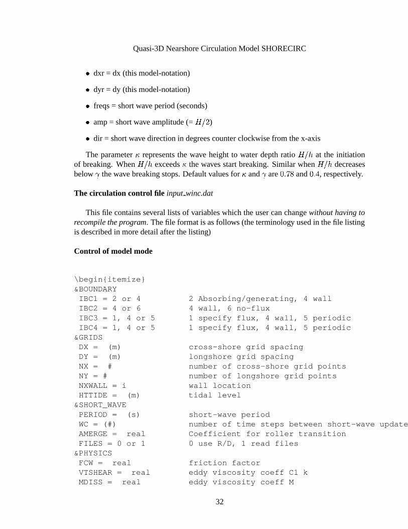
The circulation control file input winc.dat
This file containsseveral lists of variableswhich theusercanchangewithouthavingtorecompiletheprogram. Thefile formatis asfollows(theterminology usedin thefile listingis describedin moredetailafterthelisting)
Control of modelmode
\begin{itemize}&BOUNDARYIBC1 = 2 or 4 2 Absorbing/generating, 4 wallIBC2 = 4 or 6 4 wall, 6 no-fluxIBC3 = 1, 4 or 5 1 specify flux, 4 wall, 5 periodicIBC4 = 1, 4 or 5 1 specify flux, 4 wall, 5 periodic
&GRIDSDX = (m) cross-shore grid spacingDY = (m) longshore grid spacingNX = # number of cross-shore grid pointsNY = # number of longshore grid pointsNXWALL = i wall locationHTTIDE = (m) tidal level
&SHORT_WAVEPERIOD = (s) short-wave periodWC = (#) number of time steps between short-wave updatesAMERGE = real Coefficient for roller transitionFILES = 0 or 1 0 use R/D, 1 read files
&PHYSICSFCW = real friction factorVTSHEAR = real eddy viscosity coeff C1 kMDISS = real eddy viscosity coeff M
32
Quasi-3DNearshoreCirculationModelSHORECIRC
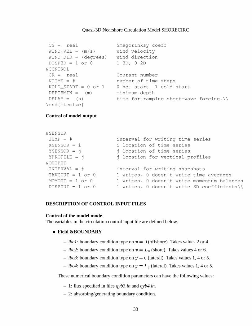
CS = real Smagorinksy coeffWIND_VEL = (m/s) wind velocityWIND_DIR = (degrees) wind directionDISP3D = 1 or 0 1 3D, 0 2D
&CONTROLCR = real Courant numberNTIME = # number of time stepsKOLD_START = 0 or 1 0 hot start, 1 cold startDEPTHMIN = (m) minimum depthDELAY = (s) time for ramping short-wave forcing.\\
\end{itemize}
Control of modeloutput
&SENSORJUMP = # interval for writing time seriesXSENSOR = i i location of time seriesYSENSOR = j j location of time seriesYPROFILE = j j location for vertical profiles
&OUTPUTINTERVAL = # interval for writing snapshotsTAVGOUT = 1 or 0 1 writes, 0 doesn’t write time averagesMOMOUT = 1 or 0 1 writes, 0 doesn’t write momentum balancesDISPOUT = 1 or 0 1 writes, 0 doesn’t write 3D coefficients\\
DESCRIPTION OF CONTROL INPUT FILES
Control of the modelmodeThevariablesin thecirculationcontrolinputfile aredefinedbelow.
: Field &BOUNDARY
– ibc1: boundarycondition typeon monpd (offshore).Takesvalues2 or 4.
– ibc2: boundarycondition typeon monpqrS (shore).Takesvalues4 or 6.
– ibc3: boundarycondition typeon stn�d (lateral).Takesvalues1, 4 or 5.
– ibc4: boundarycondition typeon stn�qrU (lateral).Takesvalues1, 4 or 5.
Thesenumericalboundaryconditionparameterscanhave thefollowing values:
– 1: flux specifiedin files qyb3.inandqyb4.in.
– 2: absorbing/generatingboundarycondition.
33
Quasi-3DNearshoreCirculationModelSHORECIRC
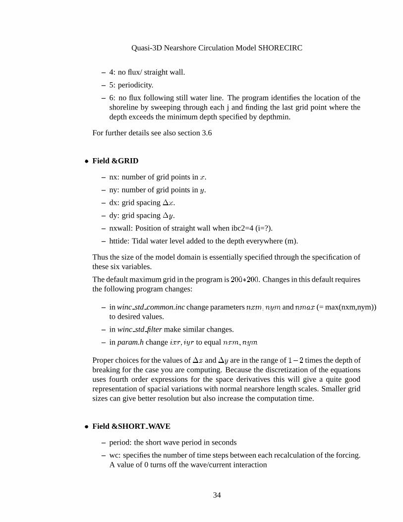
– 4: noflux/ straightwall.
– 5: periodicity.
– 6: no flux following still waterline. Theprogramidentifiesthe locationof theshorelineby sweepingthrougheachj andfinding the last grid point wherethedepthexceedstheminimumdepthspecifiedby depthmin.
For furtherdetailsseealsosection3.6
: Field &GRID
– nx: numberof grid pointsin m .
– ny: numberof grid points in s .– dx: grid spacingu�m .
– dy: grid spacinguvs .– nxwall: Positionof straightwall whenibc2=4(i=?).
– httide:Tidal waterlevel addedto thedeptheverywhere(m).
Thusthesizeof themodeldomainis essentiallyspecifiedthroughthespecificationofthesesix variables.
Thedefaultmaximumgrid in theprogramis ^ dGdKw ^ d_d . Changesin thisdefaultrequiresthefollowing programchanges:
– in winc std common.incchangeparametersxym�z3{|x}s~z andx}zo�_m (= max(nxm,nym))to desiredvalues.
– in winc std filter makesimilar changes.
– in param.hchange��m��P{|��sj� to equalxym�z3{|x}s~zProperchoicesfor thevaluesof uvm and uvs arein therangeof �}� ^ timesthedepthofbreakingfor thecaseyou arecomputing. Becausethediscretizationof theequationsusesfourth order expressionsfor the spacederivatives this will give a quite goodrepresentationof spacialvariationswith normalnearshorelengthscales.Smallergridsizescangivebetterresolution but alsoincreasethecomputation time.
: Field &SHORT WAVE
– period:theshortwaveperiodin seconds
– wc: specifiesthenumberof timestepsbetweeneachrecalculationof theforcing.A valueof 0 turnsoff thewave/currentinteraction
34
Quasi-3DNearshoreCirculationModelSHORECIRC
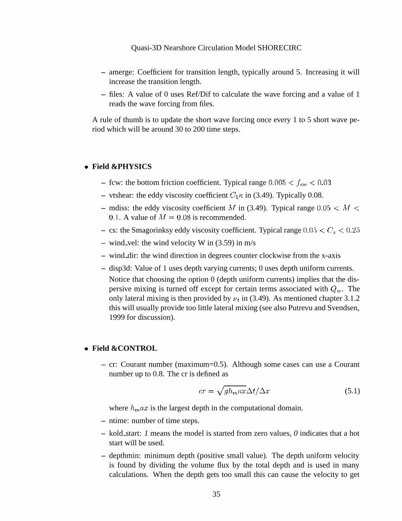
– amerge: Coefficient for transition length,typically around5. Increasingit willincreasethetransitionlength.
– files: A valueof 0 usesRef/Dif to calculatethe wave forcing anda valueof 1readsthewave forcing from files.
A rule of thumbis to updatetheshortwave forcing onceevery 1 to 5 shortwave pe-riod whichwill bearound30 to 200timesteps.
: Field &PHYSICS
– fcw: thebottomfriction coefficient. Typical rangedje�d_d_��� Q_� <3�Rdje�d_�– vtshear:theeddyviscosity coefficient ����` in (3.49).Typically 0.08.
– mdiss: theeddyviscositycoefficient � in (3.49). Typical rangedfeld������ �dfe�� . A valueof � npdfeld_i is recommended.
– cs: theSmagorinksyeddyviscositycoefficient. Typical rangedfe�d_�v�2�����Rdje ^ �– wind vel: thewind velocityW in (3.59)in m/s
– wind dir: thewind directionin degreescounterclockwisefrom thex-axis
– disp3d:Valueof 1 usesdepthvaryingcurrents;0 usesdepthuniformcurrents.
Noticethatchoosingtheoption0 (depthuniform currents)impliesthat thedis-persive mixing is turnedoff exceptfor certaintermsassociatedwith Iv< . Theonly lateralmixing is thenprovidedby ��� in (3.49).As mentionedchapter3.1.2thiswill usuallyprovide toolittle lateralmixing (seealsoPutrevu andSvendsen,1999for discussion).
: Field &CONTR OL
– cr: Courantnumber(maximum=0.5). Although somecasescanusea Courantnumberup to 0.8. Thecr is definedas
=���n�� � b A��_myu�� \ u�m (5.1)
where b Ar�_m is thelargestdepthin thecomputationaldomain.
– ntime:numberof timesteps.
– kold start:1 meansthemodelis startedfrom zerovalues,0 indicatesthata hotstartwill beused.
– depthmin:minimum depth(positive small value). The depthuniform velocityis found by dividing the volume flux by the total depthand is usedin manycalculations.Whenthe depthgetstoo small this cancausethe velocity to get
35
Quasi-3DNearshoreCirculationModelSHORECIRC
too largeandblow themodelup. Depthmin will betheminimum depthusedinall calculationspreventing this from occurring.Usevaluesaround0.01for fieldand0.001m for laboratorysimulations.
– delay:At cold startstheforcing for theflow is rampedin orderto reduceinitialoscillations andpreventinstabilities.A �V��x b W�� � \G�¡ 1¢ ��sK£ rampingwith a suitabletime constant�¡ 1¢ ��s ��¤ =�¥Px � ¤ £ is usedto phasein the forcing from zeroto fullvalue. This alsocontrolsthedelayfor computingthetime-averagedquantities:time-averagingbeginsafterdelay*5.
- Usevaluesaround40-80s for field conditions
- and10-20s for laboratorysimulations.
Makesurefor hotstartsto setthisparameterto asmallvaluesuchas0.01s.Notice that when the absorbinggeneratingboundarycondition is usedalongsomeof theboundariesany oscillationinitiatedby theupstartof themotionwillusuallypropagateoutof thesystemquitequickly. However, if theall boundariesarereflectingwalls (asin aclosedbasin)or boundarieswherethevolumeflux isspecified,thenoscillationsinitiatedatstartmaylastvery long. Suchoscillationscanbe reducedsignificantlyby choosinga valueof �¡ 1¢ �¡s which is reasonablylarge in comparisonto the basicoscillation periodsof the basin/computationaldomain. checkyour outputfor signsof basinoscillations andchose�¡ 1¢ ��s ac-cordingly.
Control of output
: Field &SENSOR
– jump: The interval (numberof time steps)which the time seriesarewritten tofiles. Typically shouldbearound10.
– xsensor:This field is a vectorthatcontainsthex-grid point numbersrequestedby the userfor the outputof time variationof ¦§ {TI¨H . (A maximum of 20 lo-cationscanbe specified. If thereare lessthan20 thenthe last oneshouldbespecifiedas0). Numbersarein grid units, between1 and x©m . Eachpair (xsen-sor(i),ysensor(i))identifiesasinglepointx andy-coordinates.
– ysensor:vectorcontainingthey-grid pointnumbersfor outputof time variationof ¦§ {TI�H . Numbersin grid units,between1 and x}s .
– yprofile: vector containing the y-grid numberfor the location for the verticalcurrentprofiles. The variation of in the cross-shoredirection of the verticalcurrentprofilesarewritten along8 sections.Must have exactly 8 j coordinates.A valueof 0 for thefirst onewill suppressthefile output
36
Quasi-3DNearshoreCirculationModelSHORECIRC
: Field &OUTPUT
– interval: interval at which “snapshots” of theflow variablesaretakenfor outputfiles.
– tavgout: Determinesif the the time-averagedpropertieswill be written to files(thefort.5xx series).A valueof 0 turnsit off anda valueof 1 turnsit on
– momout: Determinesif theinstantaneousmomentum balancewill bewritten tofiles (thefort.6xx series).A valueof 0 turnsit off anda valueof 1 turnsit on
– dispout:Determinesif the3D dispersivecoefficientswill bewritten to files (thefort.7xx series).A valueof 0 turnsit off andavalueof 1 turnsit on
5.5.2 Data input files
The data files containthe input of backgroundinformation for the modelcomputations:the bottomtopography, datafor hot startof the model,anddatafor the specifiedvolumeflux alongcross-shoreboundaries(whenthatoption is used).The following datafiles areavailable:: bath.dat: topographydatain 3 columns:x, y, depth.Theorderof thepointsis arbi-
traryandtheprogramwill checkto makesureadepthvalueis specifiedfor everygridpoint andthat thereareno duplicates.For moreinformationon topographyoptionsseeunder5.7.
: qyb3.in: (optional)Volumeflux specifiedat cross-shoreboundary3 in onecolumnstartingat monpd .
: qyb4.in: (optional)Volumeflux specifiedat cross-shoreboundary4 in onecolumnstartingat monpd .
: hot0.dat: (optional)Datafile for hot start �ªn«d . This file is automaticallygeneratedat theendof a (previous)modelrun.
: hot1.dat: (optional)Datafile for hotstart�¬n� � � . Thisfile isautomaticallygeneratedat theendof a (previous)modelrun.
: hot2.dat: (optional)Datafile for hot start �rn�� ^G� � . This file is automaticallygener-atedat theendof a (previous)modelrun.
5.6 Compiling instructions.
Important!!! For reasonsof efficiency the codeis set up to write to many datafiles inbinary form. As the first stepwhencompiling on different typesof platformsthe recordlengthfor writing directbinaryfiles mustbecheckedandadjusted.Writing to binaryfilesoccursin many locationswithin the two files winc std main.f andwinc std time.f. Do asearch-and-replacewithin thesetwo files to fix this problem. The recordlengthfor someknown platformsarelistedasfollows,
37
Quasi-3DNearshoreCirculationModelSHORECIRC
: CRAY : recl=1*ny
: SGI : recl=1*ny
: PC: recl=4*ny
: Solaris: recl=4*ny
: Digital : recl=1*ny
Compiling in Unix/LinuxThe Makefile for compiling andlinking is includedin the code. In order to createan
executablecodethreeprogramsneedto becompiled,all at onetime,usingthecommand
make shorecirc
Thenamesof theresulting threeexecutablefiles neededare
winc,createbath,createdat.
To compileonly oneof the programsusethefollowing correspondingcommandlistedbelow:
make wincmake createbathmake createdat
TheMakefilewill checkto seeif any componentof theprogramhasbeenchanged,thencompilethatfile andcreatetheexecutablefile.
Compiling in WindowsTheprogramhasbeentestedwith FortranPowerStationin Windows. To createtheexe-
cutableprogramfor generatingthetopographycompileandbuild createbath.fandwinc std common.inc.To createthe programfor generatingthe input files compileandbuild createinput.f, in-file1.f, winc std common.incand param.h. To createthe SHORECIRCexecutablepro-gramcompile andbuild winc std main.f, winc std deriv.f, winc std time.f, winc std filter.f,winc std sub1.f, infile1.f, refdif2v25a.f,winc std common.inc, param.handpass.inc.C-preprocessors
A versionof the modelutilizing C-preprocessorshasbeentested.This versionof themodelwasonly marginally fasterthanthe currentversion. Using C-preprocessorswouldrequirethatthemodelberecompiledevery time oneof theparametersis changed.Becausethe currentversionallows mostparametersto be changedwithout recompilingandis notmuchslower, wedecidednotto includethepreprocessoroptionin thisversionof themodel.
38
Quasi-3DNearshoreCirculationModelSHORECIRC
5.7 Operating procedure
Thissectionwill explain theprocedurefor runningthemodel.Thefirst stepis to createthetopographyfile bath.dat.If you want to useone of the simple topographiesdescribedin Section5.3 this can
be doneusingthe programcreatebath. This programwill interactively askfor a seriesofparametersandusethemto createthesimpletopographyof yourchoice.Theprogramwillendby creatingthe files bath.datanddim.dat. The latter file is usedby createdatwhencreatingtheinputcontrolfiles.
However, youcanalsocreateabath.datfile usingyouown topographyby following theformatdescribedin thesection5.5.2.
Thenext stepis tousetheprogramcreatedattocreatetheinputcontrolfiles input winc.datand indat.dat. This programasksinteractively what valueto usefor all the parametersinthe input files. The programwill give you the option to usethe dimensions from create-bath in thefile dim.dat. Thedetailsfor all theparametersin input winc.datarelistedin thenext section.Thedetailsfor indat.dat canbefoundin theREF/DIFmanualalthoughsomeguidelineshavebeenprovidedin thenext section.
Thecreatebathandcreatedatprogramsareprovidedfor easymeansof creatingthefilesinitially. However, againtheinputfilesdonothaveto becreatedusingthoseprograms.Youcancreatethemby handusingtheguidelinesin thenext few sections.If you only needtochangea few parametersthiscanbeaccomplishedby simply editingthefiles directly.
Themodelcanbeoperatedwith oneof two differenttypesof initial conditions: a coldstart or ahot start.
Cold StartIn a cold startthe initial conditions correspondto no flow or forcing at �®n«d . At that timetheforcingis startedbut in orderto preventunrealistic(andpotentiallyunstable)oscillationsto developtheforcingis rampedupfrom zeroat �¬n¯d to its full valueoveraperiodor sometimesteps,basedonthevalueof thedelay-parameterchosenin theinput winc.datinputfile.
Whenrunningtheprogramtherewill beaprompt
Load stresses? (0=no, 1=yes) :
By typing in 0 theprogramwill stoprunning. At this point theprogramwill have createdthe topographyandwritten it to a file called fort.311 which canbe checked to verify themodelis usingthecorrecttopography.
Thenext stepis to runtheprogramagainandcalculatetheforcingby hitting 1. Thenextpromptwill be
Start current model? (0=no, 1=yes) :
It is usuallybestto hit 0 andstoptheprogramagainto checkthat theforcing is calculatedcorrectlyby checkingtheoutputfiles describedin thenext section.
If everything checksout thentheprogramcanberun by startingtheprogramagainandhitting1 twice.
39
Quasi-3DNearshoreCirculationModelSHORECIRC
Sincemodelrunscantake a long time, a goodideais to run the programin theback-groundby usingthefollowingcommand(or something similar),
winc < screenin > screenout &
Thefile screenin containsthefollowing lines,
11
This file producesthe two keystrokesrequiredto run the model. Theotherfile, screenoutwill becreatedduringthecomputationwith all of thescreenoutputwritten to it.
Hot Start
The modelalsohasthe optionof beingoperatedfrom a hot start. A hot startrequiresinput of a setof realisticvaluesat all pointsfor the dependentvariables
§ {TItS�{T��x � I�U forthreeconsecutive time steps.Usually this informationis obtainedby storingthe valueofall variablesfrom the last threetime stepsin a previousmodelrun. Hencethe hot startisparticularlyaimedat makingit possibleto restart(andhenceextend)analreadyperformedmodelrun.
In themodelthisoptionis only providedwhenletting thecomputationrun to theendofthetime specifiedin theinput. Beforestopping themodelwill thenautomatically generatethe3 files,hot0.dat, hot1.datandhot2.dat, whichcontaintherequiredinformationfrom thelastthreetime stepsof therun. Themodelcanthenberestartedby changingtheparameterkold start to 0 andusingthosethreefiles asthe input for time steps��n°d , ��n±� � � and�vn²� ^G� � in the continuation of the previous run. Whendoing a hot startmake surethedelayis setto somesmall small valuesuchas0.01s. Otherwise,theoperatingprocedureremainsthesameasthecoldstart.
5.8 Model output
Thissectionwill describethemodeloutput,bothon thescreenandwritten to files.
5.8.1 Screenoutput
Thescreenoutputis fairly simpleandisonly reallyusefulfor debuggingpurposes.Whenthemodelis startedit will write to thescreenwhich subroutine it is working on. Theprogramalsowritesseveralof theuserdefinedparameterssotheusercanconfirmthat themodelisrunningproperly. Oncethemodelgetsto thetime loop it will write thefollowing,
Start Time Loopstep 10step 20step 30....
40
Quasi-3DNearshoreCirculationModelSHORECIRC
wherethenumberis thecurrentstep.This is repeatedevery tenstepsuntil themodelrun isdone.
Whenever themodelwritesoneof the”snapshots”thefollowing is writtento thescreen,
10001 316.1297809700816 120
wherethefirst number is thestepnumber, thesecondnumber is theactualtime associatedwith thatstepnumber, andthelastnumberis thefile which is beingcreated(seethelistingof snapshotfiles below).
Whentheprogramis doneit will write to thescreen
end
signaling thecompletionof themodelrun.
5.8.2 Output to files
The programwrites its output to files with namesfort.xxx. The xxx representsnumberswhich differentiatetheoutputfiles. Theoutputfiles arelistedasfollows with boththethe-oreticalandthe Fortranvariablenameslisted. The possible valuesof the indices(i,j) areindicatedfor eachgroupof files. Wherenothingelseis indicatedthefiles provide thepa-rametervaluesat thelasttimestepof thecomputation.
Printing out of input information
: Thefile status.datcontainsthefollowing informationdx,dy,dt,crnx,ny,ntime,interval
: Thefile numbers��³´k�µ arenotused.
Snapshotsof surfaceelevations,and depth averagedvelocities
: TimeSeriesof certainvariablesarewrittenevery jumptimesteps.Thevaluefor jumpis specifiedin input winc.dat
– �j�¶³ g�d Thesefiles will containthe time seriesof watersurfaceandvol-umefluxesat the � �·{¹¸~£ chosenfor thexsensorandysensorlocations(max20).Theoutputis
§( º �V��x � �·{¹¸~£ ), IJS ( »¼m�x � ��{¹¸~£ ), and I�U ( »¼sjx � �·{Y¸j£ ). Eachfile cor-
respondsto onesensorlocation.
: �½d_d�³ �f�½d Thesefiles containthesnapshots (up to a totalof 211)whicharetakenevery intervaltimestepsof thewatersurfaceelevation
§( º �V�¡x � ��{¹¸~£ ) andvolumefluxI�S ( »Pm�x � ��{¹¸~£ ), and I�U ( »¼sjx � ��{¹¸~£ ), respectively, at all grid points(i = 1:nx, j = 1:ny).
Thefile createdat �*n�d is numbered�1d_d . As eachnew file is createdateveryinterval,thefile number is incrementedupby 1. Thesefiles arewritten in binaryformat
41

Quasi-3DNearshoreCirculationModelSHORECIRC
: Printout of input and short wave forcing variablesis madeat all grid points � �¾n��¿�xym({¹¸ÀnÁ�¿¬x}sf£ . The constantvariables,suchastopography, areonly writtenonceat thebeginning. This appliesto theshortwave forcing whenno wave-currentinteractionis invoked. However, when utilizing wave/currentinteractionvariablessuchaswave height,changewith someinterval. Thefiles containingthosevariablesare thenoverwritten every interval time step. Hencethesefiles alwayscontainthevaluesat the last time stepof the interval-outputs. Again theseare all written inbinaryformat.
Topography information
: �j�_� topographyb�à : b � � ��{¹¸~£ .: �j� ^ Cross-shoredepthgradientsÄÆÅÆÇÄ STÈ : �~b ¥ � m�x � ��{¹¸~£ .: �j�1� LongshoredepthgradientsÄ�ÅTÇÄ U : �~b ¥ � s~x � ��{¹¸~£ .
Short wavedata
: �j�½k Shortwaveheight Ñ : Ñ � �·{¹¸~£ .: �j�P� Shortwaveanglein degrees; : � b4 �V� � ��{¹¸~£ \¼É w��½i_d .: �j�1Ê Shortwavecelerity = : = ¤½Ëv� �·{¹¸~£ .: �j�Pg Shortwave breakingindex �YÌT�GÍ � ��{¹¸~£ . Value1 meansbreakingand0 means
non-breaking.
: �j�1i Radiationstresscomponent,DESTS : DCm4m � �·{Y¸j£ .: �j�1µ Radiationstresscomponent,DESTU : DCm�s � ��{¹¸~£ .: � ^ d Radiationstresscomponent,DEU�U : DÎsjs � ��{¹¸~£ .: � ^ � �Ï Ä�Ð�ѹÑÄ S : � DCm4m � m�x �·� �·{¹¸~£ .: � ^_^ �Ï Ä�Ð�ѹÒÄ S : � DCm�s � m�x �·� �·{¹¸~£ .: � ^ � �Ï Ä�РѹÒÄ U : � DCm�s � s~x ��� ��{¹¸~£ .: � ^ k �Ï Ä�Ð�ÒYÒÄ U : � DÎs~s � s~x ��� �·{Y¸j£ .: � ^ � Shortwavebottomparticlevelocity L à : L©d � �·{Y¸j£ .: � ^ Ê Shortwavecross-shorevolumeflux I�<jS : » Ë m � ��{¹¸~£ .
42
Quasi-3DNearshoreCirculationModelSHORECIRC
: � ^ g Shortwave longshorevolume flux IJ<jU : » Ë s � ��{¹¸~£ .: � ^ i Shortwavedissipation Ó : � � ¤P¤ ��Ô��_���Õ¥¼x � �·{Y¸j£ .: � ^ µ Smoothedbreakingindex x Ë �YÌT� � �·{Y¸j£ usedwhencalculating�G� .: �G�_d Eddyviscosity ��� : Ö � � ��{¹¸~£ .
Velocity profile information: k_df��³ k�dGi Cross-shoresectionsof thecoefficientsfor theverticalvelocityprofiles
definedby equations(3.12), (3.13)and(3.22). Theselocationsarespecifiedby theinputparameteryprofile in input winc.dat. For onechosen thevariablesarewrittenout in the following orderstartingfrom the offshoreboundaryat �×n � andgoingshorewardto �,n�xym :d1x(i,j), 1x(i,j), f1x(i,j), f2x(i,j), d1y(i,j), e1y(i,j), f1y(i,j), f2y(i,j), ht(i,j), zetanp1(i,j),qxnp1(i,j),qynp1(i,j),uda4(i,j),uda3(i,j),uda2(i,j),vda4(i,j),vda3(i,j),vda2(i,j),udb4(i,j),udb3(i,j), udb2(i,j), vdb4(i,j),vdb3(i,j),vdb2(i,j),udw4(i,j),udw3(i,j),udw2(i,j),vdw4(i,j),vdw3(i,j), vdw2(i,j), udc(i,j), vdc(i,j), qwx(i,j), qwy(i,j) which provides35 columnswith nx rows. Thefiles arewritten in ASCII formatevery interval time steps,everytimeoverwriting thefiles from earliertimessothatonly thelastvaluesarekept.
Long term averagedresults.
: If tavgout= 1, thenlong term averagedvaluesof theshortwave averagedvariablesarecalculatedfrom �*np��w�Ø~Ù�ÚÜÛGÝ till theendof therun. This impliesthatunlesstotalrunningtimespecifiedfor themodelis largerthan �Cw*Ø~Ù�ÚÜÛGÝ therewill benooutputforlong termaveragedvalues.If so,awarningis written to thescreenof thecomputer.
In thefollowing ”cross-shore”referstox-components,”longshore”to they-componentsof theequations.
Theresultsarewritten in binaryformatat theendof themodelrun andcanbefoundin theoutputfiles listedbelow by their file number:
– �Gdf� Ä�Þ ÑÄ S : � � »Pm � m � ��{¹¸~£ßw���x}Ö¡à©��Ö �G�_� .– �Gd ^ Ä�Þ4ÒÄ U : � � »�s � s � �·{¹¸~£}w���x}Ö¡à©��Ö �G�_� .– �Gd_� Cross-shorebottomfriction componentáâTãÑÏ :� Q ���Õ=Æ�¹m � �·{¹¸~£,w���x}Ö�ày��Ö �G�_� .– �GdGk Cross-shoreturbulentmixing �Ï ÄÄ U ä*åà ÅÆæ N�STU � º�£ :� � �V��L � s � �·{¹¸~£(wr�Õx©Ö¡à©��Ö �G�_� .– �Gd�� Cross-shorepressuregradient� b Ä áåÄ S :� � º � m � �·{¹¸~£,w���x}Ö�à©��Ö ���_� .
43
Quasi-3DNearshoreCirculationModelSHORECIRC
– �Gd_Ê ÄÄ S � Þ Ñ·çÅ £ : ��»¼m�»Pm � m � �·{Y¸j£,wr�Õx©Ö¡à©��Ö ���_� .– �Gd�g ÄÄ U � Þ4ÑTÞ4ÒÅ £ : �¡»Pm�»¼s � s � �·{Y¸j£9w���x}Ö¡à©��Ö ����� .– �Gd_i Sumof all 3-D dispersionterms� ÄÄ S � �èSTU?£C� ÄÄ U � �èUVU1£é ÄÄ S©ê � Ó�STU
éÀë STU?£ìÄÄ S � Þ4ÑÅ £é Ó�U�U®ÄÄ U � Þ4ÑÅ £
é Ó�STS�ÄÄ S � Þ�ÒÅ £é � Ó�STU é$ë STU1£ÎÄÄ U � Þ4ÒÅ £�íé ÄÄ U ê ë U�U�ÄÄ S � Þ4ÑÅ £ é ^ Ó�STU�ÄÄ S � Þ�ÒÅ £ é � ^ Ó�U�U é$ë STU?£ÎÄÄ U � Þ4ÒÅ £�í�pÄÄ S ê�î STU�S Þ�ÑÅ é î STUVU Þ4ÒÅ í4�ÁÄÄ U êïî UVUVS Þ4ÑÅ é î UVU�U Þ4ÒÅ í :� � � ¤ Ôfm � �·{Y¸j£,wr�Õx©Ö¡ày��Ö ����� .
– �Gd_µ Longshorebottomfriction component. áâ ãÒÏ :� Q ���Õ=Æ��s � ��{¹¸~£(w���x}Ö�à©��Ö ���_� .– �j�1d Longshoreturbulentmixing. �Ï ÄÄ S ä åà ÅÆæ N�STU � º¡£ :� � �V��L � m � �·{Y¸j£ßwr�Õx©Ö¡à©��Ö ����� .– �j�_� Longshorepressuregradient.� b Ä áåÄ U :� � º � s � ��{¹¸~£ßw���x}Ö�ày��Ö ���_� .– �j� ^ ÄÄ U � Þ4Ò çÅ £ : �¡»¼s~»�s � s � �·{¹¸~£}w���x}Ö¡à©��Ö �G�_� .– �j�1� ÄÄ S � Þ4Ñ·Þ�ÒÅ £ : ��»¼m�»¼s � m � �·{¹¸~£(wr�Õx©Ö¡à©��Ö �G�_� .– �j�½k Time-averagedlongshore3-D dispersion� ÄÄ S � �èSTU?£C� ÄÄ U � �èUVU1£é ÄÄ S ê � Ó�STU éÀë STU?£ ÄÄ S � Þ ÑÅ £ é Ó�U�U ÄÄ U � Þ ÑÅ £ é Ó�STS ÄÄ S � Þ ÒÅ £ é � Ó�STU é$ë STU1£ ÄÄ U � Þ ÒÅ £�íé ÄÄ U ê ë U�U ÄÄ S � Þ ÑÅ £ é ^ Ó�STU ÄÄ S � Þ ÒÅ £ é � ^ Ó�U�U é$ë STU?£ ÄÄ U � Þ ÒÅ £�í�pÄÄ S}ê�î STU�S Þ�ÑÅ é î STUVU Þ4ÒÅ í4�ÁÄÄ U�êïî UVUVS Þ4ÑÅ é î UVU�U Þ4ÒÅ í :� � � ¤ ÔKs � �·{¹¸~£(wr�Õx©Ö¡à©��Ö �G�_� .
– �j�P� Watersurfaceelevation ¦§ : �¡º �V� � �·{¹¸~£ .– �j�1Ê Cross-shorevolumeflux I�S : ��»Pm�x � ��{¹¸~£ .– �j�Pg Longshorevolumeflux IJU : �¡»¼s~x � ��{¹¸~£ .– �j�1i ÄÄ S � Þ4Ñ Þ�ÒÅ £ calculatedfrom time-averagedquantities.
– �j�1µ ÄÄ U � Þ Ñ Þ ÒÅ £ calculatedfrom time-averagedquantities.
– � ^ d ÄÄ S � Þ4Ñ çÅ £ calculatedfrom time-averagedquantities.
– � ^ � ÄÄ U � Þ Ò çÅ £ calculatedfrom time-averagedquantities.
– � ^_^ Cross-shorepressuregradientcalculatedfrom time-averagedquantities
� b Ä áåÄ S .44
Quasi-3DNearshoreCirculationModelSHORECIRC
– � ^ � Longshorepressuregradientcalculatedfrom time-averagedquantities.
� b Ä áåÄ U .– � ^ k Cross-shorebottomfriction calculatedfrom time-averagedquantities.
– � ^ � Longshorebottomfriction calculatedfrom time-averagedquantities
Terms in the instantaneousmomentum balance
: If momout= 1, thentermsin theinstantaneousmomentumbalancearewritten everyinterval time steps.Written in binaryformat.
– Ê_df� � �Ï Ä�Ð�ѹÑÄ S : � Q ¥P��= m4m � ��{¹¸_{·��£ .– Ê_d ^ � �Ï Ä�РѹÒÄ U : � Q ¥¼��= m�s � ��{¹¸_{·��£ .– Ê_d_� Cross-shorebottomfriction component� áâ ãÑÏ : � Q �¼�Y=T�¹m � �·{Y¸j£ .– Ê_dGk Cross-shoreturbulentmixing �Ï ÄÄ U ä åà ÅÆæ N�STU � º�£ : � �V�¡L4m � s � �·{Y¸j£ .– Ê_d�� Cross-shorepressuregradient�ª� b Ä áåÄ S : �ª� w b �¹� � ��{¹¸~£4w � º �V� � m ¤ �V�¡� � ��{¹¸~£ .– Ê_d_Ê Cross-shorenonlinearconvective terms � ÄÄ S � Þ Ñ çÅ £C� ÄÄ U � Þ Ñ Þ ÒÅ £ :��»Pm�»¼m � m � �·{¹¸~£Î�ð»¼m�»¼s � s � ��{¹¸~£ .– Ê_d�g � �Ï Ä�Ð�ѹÒÄ S : � Q ¥¼��= m�s � ��{¹¸_{·��£ .– Ê_d_i � �Ï Ä�Ð�ÒYÒÄ U : � Q ¥P�G= sjs � ��{¹¸_{·��£ .– Ê_d_µ Longshorebottomfriction component. � �Ï áâ ãÒÏ : � Q ���Õ=Æ��s � ��{¹¸~£ .– Êf�1d Longshoreturbulentmixing �Ï ÄÄ S ä åà ÅÆæ N�STU � º¡£ : � �V��L4m � m � �·{Y¸j£ .– Êf�_� Longshorepressuregradient�®� b Ä áåÄ U : �ª��w b �¹� � ��{¹¸~£,w � º �V� � s ¤ �V��� � �·{Y¸j£ .– Êf� ^ Longshorenonlinearconvective terms �pÄÄ U � Þ4Ò çÅ £C�ñÄÄ S � Þ4ÑTÞ4ÒÅ £ :��»Pm�»�s � m � ��{¹¸~£C�ð»�s~»�s � s � �·{¹¸~£ .– Êf�1� Cross-shore3-D dispersion� ÄÄ S � �èSTS1£C� ÄÄ U � �èSTU1£é ÄÄ S©ê � ^ Ó�STS é$ë STS1£ìÄÄ S � Þ ÑÅ £ é ^ Ó�STU®ÄÄ U � Þ ÑÅ £ éÀë STS�ÄÄ U � Þ4ÒÅ £¹íé ÄÄ U�ê � Ó�STU éÀë STU?£ìÄÄ S � Þ4ÑÅ £ é Ó�U�U®ÄÄ U � Þ4ÑÅ £ é Ó�STS�ÄÄ S � Þ�ÒÅ £ é � Ó�STU é$ë STU½£*ÄÄ U � Þ�ÒÅ £�í�´ÄÄ S êïî STSTS Þ4ÑÅ é î STSTU Þ4ÒÅ íK�ÁÄÄ U êïî STUVS Þ4ÑÅ é î STUVU Þ�ÒÅ í :� � ¤ ÔKm � ��{¹¸~£ .– Êf�½k Longshore3-D dispersion� ÄÄ S � �èSTU?£C� ÄÄ U � �èUVU1£é ÄÄ S©ê � Ó�STU é$ë STU1£*ÄÄ S � Þ4ÑÅ £ é Ó�UVU®ÄÄ U � Þ4ÑÅ £ é Ó�STS�ÄÄ S � Þ ÒÅ £ é � Ó�STU é$ë STU½£ÎÄÄ U � Þ ÒÅ £¹í
45
Quasi-3DNearshoreCirculationModelSHORECIRC
é ÄÄ U ê ë UVU�ÄÄ S � Þ�ÑÅ £ é ^ Ó�STU®ÄÄ S � Þ4ÒÅ £ é � ^ ÓvUVU éÀë STU?£*ÄÄ U � Þ4ÒÅ £¹í�´ÄÄ S êïî STUVS Þ4ÑÅ é î STU�U Þ4ÒÅ íK�ÁÄÄ U êïî UVU�S Þ4ÑÅ é î U�UVU Þ�ÒÅ í :� � ¤ Ô4s � �·{¹¸~£ .– Êf�P� Cross-shorelocalacceleration� Ä�Þ ÑÄ � : � � »Pm�xjÔE� � �·{Y¸j£Î�ð»Pm�x � �·{¹¸~£·£ \G� � .– Êf�1Ê Longshorelocalacceleration� Ä�Þ ÒÄ � : � � »¼s~xjÔE� � �·{¹¸~£,�ð»¼s~x � ��{¹¸~£·£ \G� � .– Êf�Pg ÄÄ S � Þ Ñ·çÅ £ :»¼m�»Pm � m � �·{Y¸j£ .– Êf�1i ÄÄ U � Þ4ÑTÞ4ÒÅ £ : »¼m�»¼s � s � ��{¹¸~£ .– Êf�1µ ÄÄ U � Þ Ò çÅ £ :»�s~»�s � s � �·{¹¸~£ .– Ê ^ d ÄÄ S � Þ4Ñ·Þ�ÒÅ £ : »Pm�»�s � m � �·{Y¸j£ .– Ê ^ � Cross-shorewind stress
âÆòÑÏ : Ë ��x � S � ��£ .– Ê ^_^ Longshorewind stress
âÆòÒÏ : Ë ��x � U � ��£ .: g�df� Position of the lastwet point x©my� � ��{¹¸~£ written in ASCII every interval time
steps.
The valuesof the dispersivemixing coefficients.
: Whenthemodelis run in quasi-3Dmodeanddispout= 1, thenthedispersivemixingcoefficientsarewritten every interval time steps.Theseresultsarewritten in binaryformaton thefollowing files (whichareoverwrittenat eachinterval time steps):
– g�k�Ê ë B½H : ë m4m � ��{¹¸~£ , ë m�s � ��{¹¸~£ , ë s~s � �·{Y¸j£– g�k¡g ÓvB½H : Óóm4m � �·{¹¸~£ , Óóm�s � �·{¹¸~£ , Óas~s � �·{¹¸~£– g�k�i ��B½H : �ôm4m � �·{Y¸j£ , �¯m�s � �·{Y¸j£ , ��s~s � �·{¹¸~£– g�k�µ î B½H?S : î m4m4m � �·{¹¸~£ , î m�s~m � �·{¹¸~£ ,î s~s~m � �·{¹¸~£– g�k�µ î B½H?U : î m4m�s � �·{¹¸~£ , î m�sjs � ��{¹¸~£ ,î s~sjs � ��{¹¸~£
Data for next hot start
– hot0.dat, hot1.datandhot2.datarecreatedat theendof everymodelrunandcanbeusedfor a hot start.They containwaterlevelsandvolume fluxesfor thelastthreetimesteps.
46
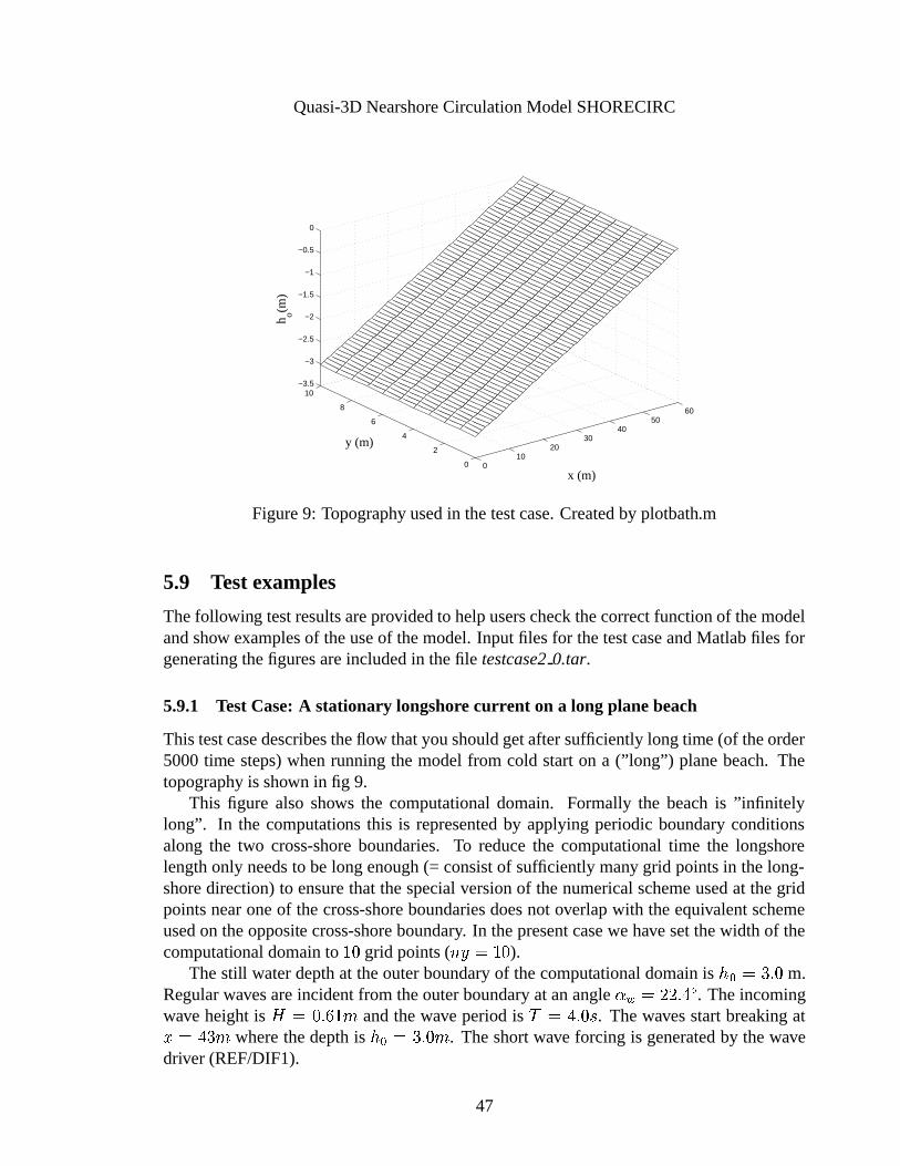
Quasi-3DNearshoreCirculationModelSHORECIRC
010
2030
4050
60
0
2
4
6
8
10−3.5
−3
−2.5
−2
−1.5
−1
−0.5
0
x (m)
y (m)
h o(m)
Figure9: Topographyusedin thetestcase.Createdby plotbath.m
5.9 Testexamples
Thefollowing testresultsareprovidedto helpuserscheckthecorrectfunctionof themodelandshow examplesof theuseof themodel.Input files for thetestcaseandMatlabfiles forgeneratingthefiguresareincludedin thefile testcase20.tar.
5.9.1 TestCase:A stationary longshorecurrent on a long planebeach
This testcasedescribestheflow thatyoushouldgetaftersufficiently longtime(of theorder5000time steps)whenrunningthe modelfrom cold starton a (”long”) planebeach.Thetopographyis shown in fig 9.
This figure also shows the computationaldomain. Formally the beachis ”infinitelylong”. In the computations this is representedby applyingperiodicboundaryconditionsalong the two cross-shoreboundaries. To reducethe computational time the longshorelengthonly needsto belongenough(= consistof sufficiently many grid pointsin thelong-shoredirection)to ensurethat thespecialversionof thenumericalschemeusedat thegridpointsnearoneof thecross-shoreboundariesdoesnot overlapwith theequivalentschemeusedon theopposite cross-shoreboundary. In thepresentcasewe have setthewidth of thecomputationaldomainto �1d grid points( x}s×n��½d ).
Thestill waterdepthat theouterboundaryof thecomputationaldomainis b M�n�je�d m.Regularwavesareincidentfrom theouterboundaryat anangle;,<¾n ^_^ eõk�ö . Theincomingwave heightis ÷´nødfelÊf�½z andthewave periodis ù�nøkKeld ¤ . Thewavesstartbreakingatm3n«k��Gz wherethedepthis b M�n«�feldGz . Theshortwave forcing is generatedby thewavedriver (REF/DIF1).
47
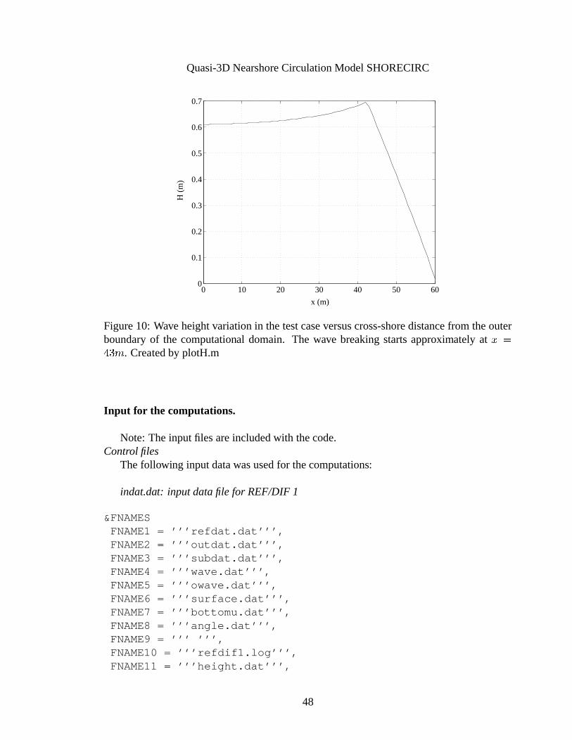
Quasi-3DNearshoreCirculationModelSHORECIRC
0 10 20 30 40 50 600
0.1
0.2
0.3
0.4
0.5
0.6
0.7
x (m)
H (
m)
Figure10: Wave heightvariationin thetestcaseversuscross-shoredistancefrom theouterboundaryof the computational domain. The wave breakingstartsapproximately at múnk���z . Createdby plotH.m
Input for the computations.
Note:Theinputfiles areincludedwith thecode.Control files
Thefollowing inputdatawasusedfor thecomputations:
indat.dat: inputdatafile for REF/DIF1
&FNAMESFNAME1 = ’’’refdat.dat’’’,FNAME2 = ’’’outdat.dat’’’,FNAME3 = ’’’subdat.dat’’’,FNAME4 = ’’’wave.dat’’’,FNAME5 = ’’’owave.dat’’’,FNAME6 = ’’’surface.dat’’’,FNAME7 = ’’’bottomu.dat’’’,FNAME8 = ’’’angle.dat’’’,FNAME9 = ’’’ ’’’,FNAME10 = ’’’refdif1.log’’’,FNAME11 = ’’’height.dat’’’,
48
Quasi-3DNearshoreCirculationModelSHORECIRC
FNAME12 = ’’’sxx.dat’’’,FNAME13 = ’’’sxy.dat’’’,FNAME14 = ’’’syy.dat’’’,FNAME15 = ’’’depth.dat’’’/
&INGRIDMR = 61,NR = 11,IU = 1,NTYPE = 0,ICUR = 1,IBC = 1,ISMOOTH = 0,DXR = 1.,DYR = 1.,DT = 0.005,ISPACE = 0,ND = 1,IFF = 1 0 0,ISP = 0,IINPUT = 1,IOUTPUT = 1/
&WAVES1AIWAVE = 1,NFREQS = 1,KAPP = 0.78,GAMM = 0.4/
&WAVES1BFREQS = 4.,TIDE = 0.,NWAVS = 1,AMP = 0.305,DIR = 22.4/
input winc.dat: Inputdatafile for circulationpart of themodel.
&BOUNDARYIBC1 = 2,IBC2 = 4,IBC3 = 5,IBC4 = 5/
&GRIDSDX = 1.,DY = 1.,
49
Quasi-3DNearshoreCirculationModelSHORECIRC
NX = 61,NY = 11,NXWALL = 61,HTTIDE = 0./
&SHORT_WAVEPERIOD = 4.,WC = 0,AMERGE = 5.,FILES = 0/
&PHYSICSFCW = 0.012,VTSHEAR = 0.08,MDISS = 0.05,CS = 0.2,WIND_VEL = 0.,WIND_DIR = 0.,DISP3D = 1/
&CONTROLCR = 0.5,NTIME = 5001,KOLD_START = 1,DEPTHMIN = 0.002,DELAY = 40./
&SENSORJUMP = 10,XSENSOR = 0 0 0 0 0 0 0 0 0 0 0 0 0 0 0 0 0 0 0 0,YSENSOR = 0 0 0 0 0 0 0 0 0 0 0 0 0 0 0 0 0 0 0 0,YPROFILE = 5 0 0 0 0 0 0 0/
&OUTPUTINTERVAL =100,TAVGOUT = 0,MOMOUT = 0,DISPOUT = 1/
DatafilesThebottom topographyis a planebeachwith a slopeof 1:20which is generatedby
usingtheprogramcreatebathdescribedin Sections5.3and5.7. Theshorelineis at x = 60m.
Results.
Theresultsfrom thecomputationsareshown in thefollowingfigures.They areobtainedafter �GdGd_d timestepsandrepresentthenearlysteadyflow conditions.
50
Quasi-3DNearshoreCirculationModelSHORECIRC
0 10 20 30 40 50 600
0.2
0.4
0.6
0.8
1
1.2
cross−shore distance (m)
long
−sh
ore
curr
ent (
m/s
)
Figure11: Thelongshorevelocities û@ for thetestcaseversuscross-shoredistance.Createdby currentV.m
Thewaveheightvariationin thecross-shoredirectionis shown in fig 10. Similarly, Fig11 shows thecross-shoredistribution of thelongshorecurrents û@ . Theverticalvariationofthe velocitiesarea combination of the the depthvarying undertow andthe depthvaryinglongshore currents.Fig 12 shows thevariationof thecross-andlongshorevelocities overdepth(left two panels)andthe3-D profilesof thetotal currentsvelocitiesat four differentcross-shorepositions(right panel).Thetop 2 rows areoutsidethesurfzoneandthebottom2 rowsareinsidethesurfzone.Thesameprofilesareshown with thetopographyin Fig 13.
5.9.2 Example: Cold start of longshorecurr ent on a long planebeach
The purposeof this exampleis to demonstratethe capabilitiesof the modelto handlethecomplexitiesof aseeminglysimplecase.Thesituationconsideredin thisexample is thecoldstartof a longshore currentona longstraightcoast.This is thesamesituation thatwasanalysedby VanDongerenetal (1994).However, becausethemodelhasdevelopedconsid-erablysincethentheactualresultsdiffer somewhat from theresultsof thatpublication.
Thisexampleis essentially thesameflow situation thatwasshown in Example1 above.However, in thepresentexamplewe examinetheflow in time asit develops from thecoldstart. The idea is to illustratehow complicatedthe detailsof the flow patternareuntil iteventually reachestherelatively simplesteadysituationshown in thetestcase.Despitethecomplicatedbehavior, theflow remainslongshoreuniform throughout thedevelopment tothesteadystate.
This example demonstratesall partsof themodelexceptthevariationsin thelongshore
51
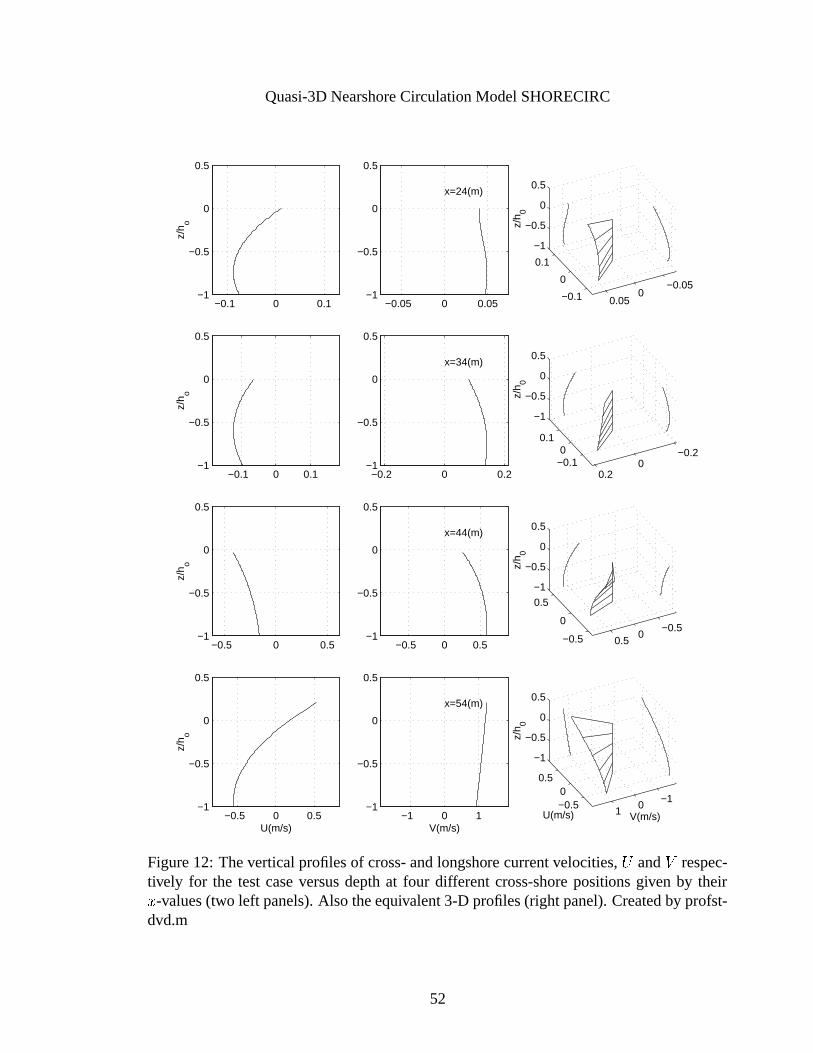
Quasi-3DNearshoreCirculationModelSHORECIRC
−0.1 0 0.1−1
−0.5
0
0.5z/
h o
−0.05 0 0.05−1
−0.5
0
0.5
x=24(m)
−0.1
0
0.1
−0.050
0.05
−1
−0.5
0
0.5
z/h 0
−0.1 0 0.1−1
−0.5
0
0.5
z/h o
−0.2 0 0.2−1
−0.5
0
0.5
x=34(m)
−0.10
0.1−0.2
00.2
−1
−0.5
0
0.5
z/h 0
−0.5 0 0.5−1
−0.5
0
0.5
z/h o
−0.5 0 0.5−1
−0.5
0
0.5
x=44(m)
−0.5
0
0.5
−0.50
0.5
−1
−0.5
0
0.5z/
h 0
−0.5 0 0.5−1
−0.5
0
0.5
U(m/s)
z/h o
−1 0 1−1
−0.5
0
0.5
V(m/s)
x=54(m)
−0.50
0.5
−10
1
−1
−0.5
0
0.5
V(m/s)U(m/s)
z/h 0
Figure12: Theverticalprofilesof cross-andlongshore currentvelocities, ü and @ respec-tively for the testcaseversusdepthat four differentcross-shorepositionsgiven by theirm -values(two left panels).Also theequivalent3-D profiles(right panel).Createdby profst-dvd.m
52
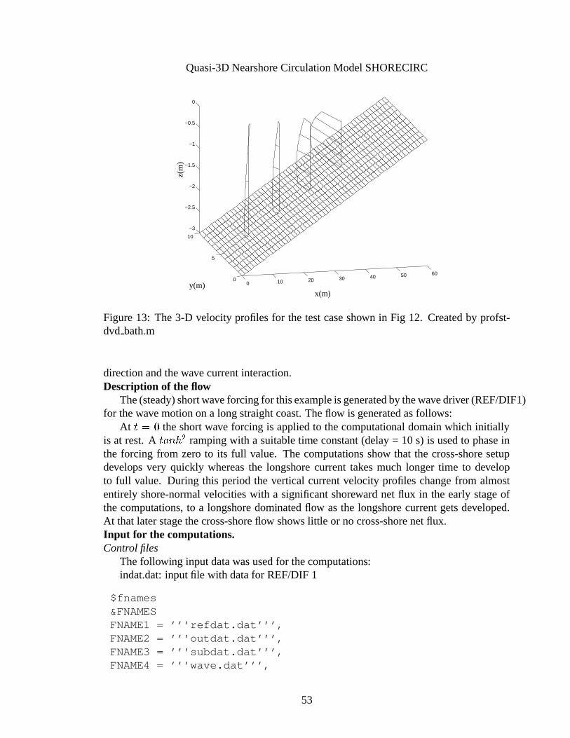
Quasi-3DNearshoreCirculationModelSHORECIRC
0 10 20 30 40 50 600
5
10
−3
−2.5
−2
−1.5
−1
−0.5
0
x(m)y(m)
z(m
)
Figure13: The3-D velocity profilesfor the testcaseshown in Fig 12. Createdby profst-dvd bath.m
directionandthewavecurrentinteraction.Description of the flow
The(steady)shortwaveforcingfor thisexampleisgeneratedby thewavedriver (REF/DIF1)for thewavemotionona longstraightcoast.Theflow is generatedasfollows:
At �ªn�d theshortwave forcing is appliedto thecomputational domainwhich initiallyis at rest. A �V��x b W rampingwith a suitabletime constant(delay= 10 s) is usedto phaseinthe forcing from zeroto its full value. The computationsshow that the cross-shoresetupdevelops very quickly whereasthe longshore currenttakesmuch longer time to developto full value. During this periodthe vertical currentvelocity profileschangefrom almostentirely shore-normalvelocities with a significantshoreward net flux in the early stageofthe computations,to a longshore dominatedflow asthe longshorecurrentgetsdeveloped.At thatlaterstagethecross-shoreflow shows litt le or nocross-shorenetflux.Input for the computations.Control files
Thefollowing inputdatawasusedfor thecomputations:indat.dat:inputfile with datafor REF/DIF1
$fnames&FNAMESFNAME1 = ’’’refdat.dat’’’,FNAME2 = ’’’outdat.dat’’’,FNAME3 = ’’’subdat.dat’’’,FNAME4 = ’’’wave.dat’’’,
53
Quasi-3DNearshoreCirculationModelSHORECIRC
FNAME5 = ’’’owave.dat’’’,FNAME6 = ’’’surface.dat’’’,FNAME7 = ’’’bottomu.dat’’’,FNAME8 = ’’’angle.dat’’’,FNAME9 = ’’’ ’’’,FNAME10 = ’’’refdif1.log’’’,FNAME11 = ’’’height.dat’’’,FNAME12 = ’’’sxx.dat’’’,FNAME13 = ’’’sxy.dat’’’,FNAME14 = ’’’syy.dat’’’,FNAME15 = ’’’depth.dat’’’/
&INGRIDMR = 61,NR = 11,IU = 1,NTYPE = 0,ICUR = 1,IBC = 1,ISMOOTH = 0,DXR = 1.,DYR = 1.,DT = 0.005,ISPACE = 0,ND = 1,IFF = 1 0 0,ISP = 0,IINPUT = 1,IOUTPUT = 1/
&WAVES1AIWAVE = 1,NFREQS = 1,KAPP = 0.78,GAMM = 0.4/
&WAVES1BFREQS = 4.,TIDE = 0.,NWAVS = 1,AMP = 0.305,DIR = 22.4/
input winc.dat: Inputdatafile for circulationpart of themodel.
&BOUNDARY
54
Quasi-3DNearshoreCirculationModelSHORECIRC
IBC1 = 2,IBC2 = 4,IBC3 = 5,IBC4 = 5/
&GRIDSDX = 1.,DY = 1.,NX = 61,NY = 11,NXWALL = 61,HTTIDE = 0./
&SHORT_WAVEPERIOD = 4.,WC = 0,AMERGE = 5.,FILES = 0/
&PHYSICSFCW = 0.012,VTSHEAR = 0.08,MDISS = 0.05,CS = 0.2,WIND_VEL = 0.,WIND_DIR = 0.,DISP3D = 1/
&CONTROLCR = 0.5,NTIME = 5001,KOLD_START = 1,DEPTHMIN = 0.002,DELAY = 10./
&SENSORJUMP = 10,XSENSOR = 0 0 0 0 0 0 0 0 0 0 0 0 0 0 0 0 0 0 0 0,YSENSOR = 0 0 0 0 0 0 0 0 0 0 0 0 0 0 0 0 0 0 0 0,YPROFILE = 5 0 0 0 0 0 0 0/
&OUTPUTINTERVAL =47,TAVGOUT = 0,MOMOUT = 0,DISPOUT = 1/
Results.Thefollowing resultsareshown from thecomputations:
55
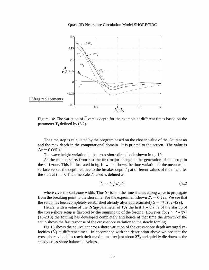
Quasi-3DNearshoreCirculationModelSHORECIRC
0 0.5 1 1.5 2−0.1
−0.05
0
0.05
0.1
0.15
0.2
Tb/2
Tb
2Tb
4Tb
8Tb
16Tb
25Tb
PSfragreplacements
ýþ ÿ��
b M \Gb��
Figure14: Thevariationof§
versusdepthfor theexampleat differenttimesbasedon theparameterù � definedby (5.2).
Thetime stepis calculatedby theprogrambasedon thechosenvalueof theCourantnoandthe max depthin the computational domain. It is printedto the screen.The valueisu��¬n�dfe�dGÊ�� ¤
Thewaveheightvariation in thecross-shoredirectionis shown in fig 10.As the motion startsfrom rest the first major changeis the generationof the setupin
thesurf zone.This is illustratedin fig 10which shows thetime variationof themeanwatersurfaceversusthedepthrelative to thebreaker depth b�� at differentvaluesof thetime afterthestartat �*n�d . Thetimescaleù � usedis definedas
ù � n�q �V\ � � b�� (5.2)
whereq � is thesurfzonewidth. Thusù � is half thetimeit takesalongwaveto propagatefrom thebreakingpoint to theshoreline.For theexperimentshown ù � npÊje�� ^ ¤ . Weseethatthesetuphasbeencompletelyestablishedalreadyafterapproximately���ðg¼ù � (32-45s).
Hence,with a valueof the �¡ 1¢ ��s -parameterof �1d ¤ thefirst � � ^ w®ù � of thestartupofthecross-shoresetupis flavoredby therampingupof theforcing. However, for ��� ^ � ��ù �(15-20s) the forcing hasdevelopedcompletelyandhenceat that time the growth of thesetupshowsthefastresponseof thecross-shorevariation to thesteadyforcing.
Fig 15 shows theequivalentcross-shorevariation of thecross-shoredepthaveragedve-locities ( ûü ) at different times. In accordancewith the description above we seethat thecross-shorevelocitiesreachtheirmaximumafterjustabout ù � andquickly diedown asthesteadycross-shorebalancedevelops.
56

Quasi-3DNearshoreCirculationModelSHORECIRC
0 0.5 1 1.5 2−0.02
0
0.02
0.04
0.06
0.08
0.1
Tb/2
Tb
2Tb
8Tb
4Tb 16T
b PSfragreplacements
�þ� �ÿ��
b M \Gb��
Figure15: The cross-shorevelocities ûü \� � b�� versusdepthfor the exampleat differenttimesbasedon theparameterù � definedby (5.2).
In contrastto the cross-shoreflow, the longshore flow develops quite slowly. Fig 16shows the longshorecurrentvelocities. Here the timescalefor the growth of the flow isclearlymuchlonger. Evenafter �1Ê�ù � ( � �1dGd ¤ ) thevelocity hasonly reachedabout i���� ofthefull value.
I may be worth mentioning that, becausewe usea periodicboundaryconditionin thelongshoredirectionthereareno longshoreoscillationsfrom thestartup. If, however, a fluxcondition is specifiedateachof thecross-shoreboundariesthiswouldneedto berampedupatthesamerateasthestart-upratefor thelongshoreuniformlongshorecurrentin themiddleof the computational domainin order to prevent longshoreoscillations to develop. Suchoscillationswouldtypically haveatimescaleof ù���npqÎU \� � b�� whichcouldbemuchlongerthan ù � . Furthermore,sincecross-shoreboundarieswith a flux conditionwill fully reflectall (oscillatory) deviationsfrom the specifiedflux, suchoscillationswill generallyremainpresentfor a long time and essentiallyonly propagateout of the computational domainthroughthe absorbingoffshoreboundary(as they turn into 2DH oscillations due to thecross-shoredepthvariation).
As mentionedthevelocitiesshown in thepreviousfiguresaredepthaveragedvelocities.However, the actualvelocitiesvary over depth. Fig 17 shows the verticalprofilesat threedifferentpositions(at b�\_b�� n �Geh� , �_eld and dfe ^ � ) at threedifferenttimes( ��n ^ ù � , ʼù � , and^ d¼ù � respectively).
At b�\_b�� n �_e�� , which is well outside the surf zonethe longshorevelocities arequitesmallandthecross-shorevelocitiesdominate.
Around the breakingpoint the two velocity components areof the sameorderbut not
57
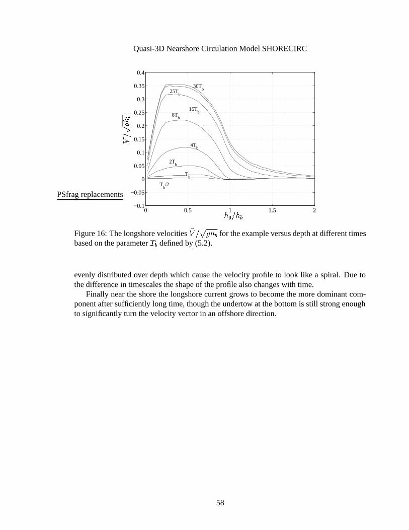
Quasi-3DNearshoreCirculationModelSHORECIRC
0 0.5 1 1.5 2−0.1
−0.05
0
0.05
0.1
0.15
0.2
0.25
0.3
0.35
0.4
Tb/2
Tb
2Tb
4Tb
8Tb
16Tb
25Tb
30Tb
PSfragreplacements
��þ� �ÿ �
b M \Gb��
Figure16: Thelongshorevelocities û@ \� � b�� for theexampleversusdepthatdifferenttimesbasedon theparameterù � definedby (5.2).
evenly distributedover depthwhich causethevelocity profile to look like a spiral. Duetothedifferencein timescalestheshapeof theprofilealsochangeswith time.
Finally neartheshorethe longshorecurrentgrows to becomethemoredominantcom-ponentaftersufficiently long time,thoughtheundertow at thebottomis still strongenoughto significantlyturn thevelocity vectorin anoffshoredirection.
58
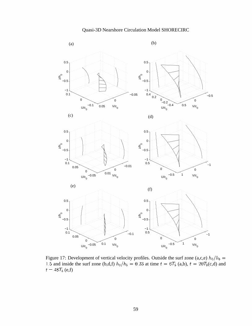
Quasi-3DNearshoreCirculationModelSHORECIRC
−0.050
0.050.1
−0.010
0.01
−1
−0.5
0
0.5
V/c0U/c
0
z/h 0
−0.1
0
0.1 −0.05
0
0.05
−1
−0.5
0
0.5
V/c0U/c
0
z/h 0
−0.4−0.2
00.2
0.4 −0.5
0
0.5
−1
−0.5
0
0.5
V/c0U/c
0
z/h 0
−0.5
0
0.5 −1
0
1
−1
−0.5
0
0.5
V/c0U/c
0
z/h 0
−0.5
0
0.5−1
0
1
−1
−0.5
0
0.5
V/c0U/c
0
z/h 0
−0.050
0.050.1 −0.1
0
0.1
−1
−0.5
0
0.5
V/c0U/c
0
z/h 0
(a) (b)
(c) (d)
(f) (e)
Figure17: Developmentof verticalvelocityprofiles.Outsidethesurf zone(a,c,e)b M \_b�� n�_e�� andinside thesurf zone(b,d,f) b M \_b�� n�dfe ^ � at time � n�Ê�ù � (a,b), � n ^ d�ù � (c,d) and�*n¯k�i�ù � (e,f)
59
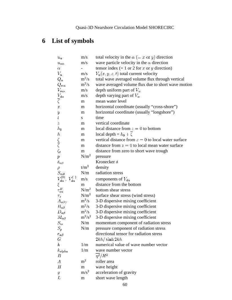
Quasi-3DNearshoreCirculationModelSHORECIRC
6 List of symbols
LyB m/s total velocity in the ; � nôm����*sf£ directionL�<fB m/s waveparticlevelocity in the ; direction; - tensorindex (= 1 or 2 for m or s direction)@�B m/s @yB � m({|sy{Tºf{·��£ total currentvelocityI�B mW /s totalwaveaveragedvolumeflux throughverticalI¨<fB mW /s waveaveragedvolumeflux dueto shortwavemotion@4A,B m/s depthuniformpartof @}B@���B m/s depthvaryingpartof @©B§m meanwaterlevelm m horizontalcoordinate(usually“cross-shore”)s m horizontalcoordinate(usually“longshore”)� s timeº m verticalcoordinateb M m localdistancefrom ºJnpd to bottomb m localdepth= b M é §§m verticaldistancefrom ºJnpd to localwatersurface§m distancefrom º�n�d to localmeanwatersurface§ � m distancefrom zeroto shortwave troughÔ N/mW pressure� B½H Kronecker
�� t/m� densityD}BPO N/m radiationstress@�� M ���B {r@!� �"���B m/s componentsof @#��B$
m distancefrom thebottomN OB½S N/mW bottomshearstressN½� N/mW surfaceshearstress(wind stress)
î B½H&% mW /s 3-D dispersivemixing coefficientë B½H mW /s 3-D dispersivemixing coefficientÓtB½H mW /s 3-D dispersivemixing coefficient��B½H m� /sW 3-D dispersivemixing coefficientD©A N/m momentumcomponentof radiationstressD(' N/m pressurecomponentof radiationstress B½H directionaltensorfor radiationstress) ^ Í b�\+*-,/.�0ª^ Í bÍ 1/m numericalvalueof wavenumber vectorÍ213� ' Å 1 1/m wavenumbervectorë 4 W \ ÷ Wî mW roller area÷ m waveheight� m/sW accelerationof gravityq m shortwave length
60
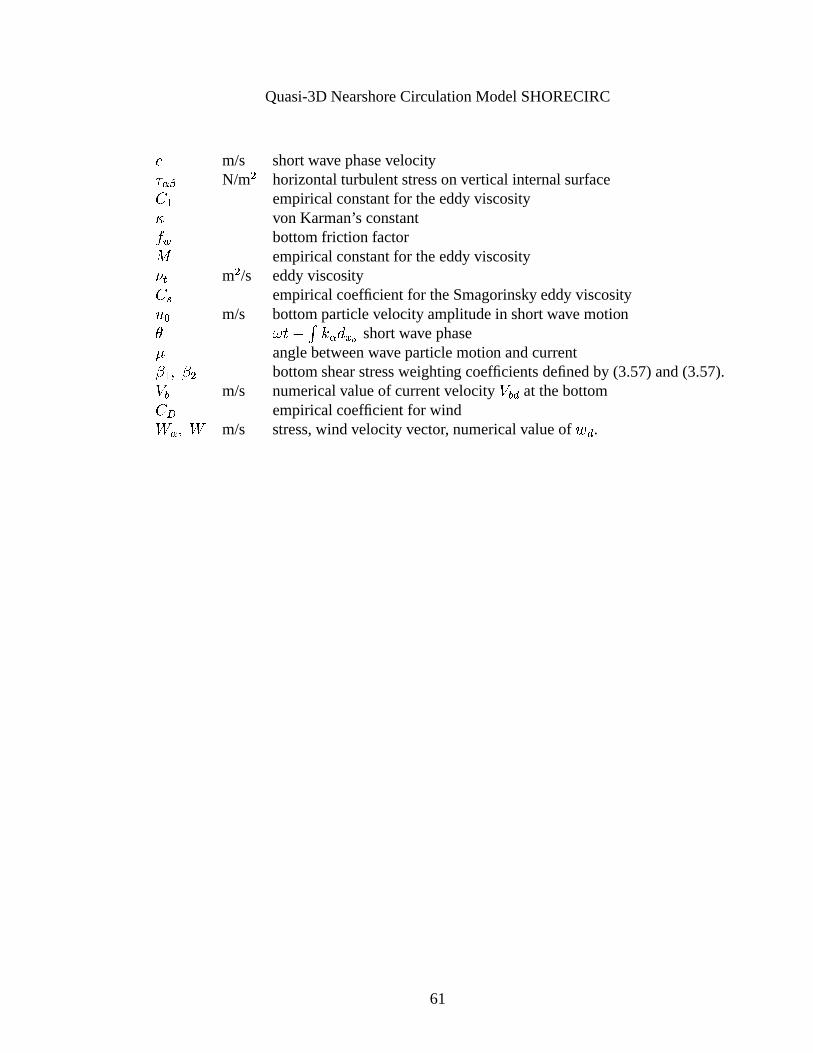
Quasi-3DNearshoreCirculationModelSHORECIRC
= m/s shortwavephasevelocityN�B½H N/mW horizontalturbulentstressonverticalinternalsurface��� empiricalconstantfor theeddyviscosity` vonKarman’s constantQ < bottomfriction factor� empiricalconstantfor theeddyviscosity�1� mW /s eddyviscosity� � empiricalcoefficient for theSmagorinsky eddyviscosityL�M m/s bottomparticlevelocityamplitudein shortwavemotion5 6 �,� ä Í�B � S È shortwavephase7 anglebetweenwaveparticlemotion andcurrent8 �Æ{ 8 W bottomshearstressweighting coefficientsdefinedby (3.57)and(3.57).@ � m/s numericalvalueof currentvelocity @ � � at thebottom�:9 empiricalcoefficient for wind; BK{ ;m/s stress,wind velocityvector, numericalvalueof Ë � .
61
Quasi-3DNearshoreCirculationModelSHORECIRC
7 List of references< Battjes,J. A. (1975): Modeling of turbulencein the surf zone. ASCEProc. Symp. on Modelling
Techniques, SanFrancisco,1050-1061.< Church, J.C.andE. B. Thornton (1993): Effects of breaking wave inducedturbulencewithin a long-
shorecurrent model.CoastalEngineering20, 1-28.< Coffey, F.C. andP. Nielsen(1984): Aspectsof wave currentboundarylayerflows. In Proc.,19thInt.
Conf. onCoast.Engrg., ASCE,2232-2245.< Drei, E. , A. Lamberti, andI. A. Svendsen(2000). Currentanalysisaround a submergedbreakwater.
Proc.IVth Int. Conf. Hydrodyn. Yokohama,(edsGoda, Ikehata,Suzuki). 693– 698< Haas,K. andI.A. SvendsenandM.C. Haller (1998): Numericalmodelingof nearshorecirculation on
abarredbeachwith rip channels. In Proc.,26thInt. Conf. onCoast.Engrg., ASCE,801-814.< Haas,K. A. & I. A. Svendsen(2000a).Three-dimensional modelling of rip currentsystems.Rep.No.
CACR-00-06, 250pp.< Haas,K. A. , I. A. Svendsen(2000b). 3-D modeling of rip currents. ICCE2000, Sydney, Australia,< Haas,K. A. , I. A. Svendsen(2002). Laboratorymeasurementsof theverticalstructure of rip currents.
To appearin JGR.< Haas,K. A. , I. A. Svendsen,M. C. Haller andQ. Zhao(2002). Quasi3-D modelling of rip currents:
horizontalproperties.Submitted for publication.< Hansen,J.B. (1990)Periodicwavesin thesurfzone:Analysisof experimentaldataCoastalEngineer-
ing. 14, 19–41.< Kirby, J.T. andR.A. Dalrymple (1994): Combinedrefraction/diffractionmodel REF/DIF1,Version
2.5. Res.ReportCACR-94-22, Centerfor AppliedCoastalResearch,Univ. of Delaware.< Longuet-Higgins,M.S. (1956): Themechanicsof theboundary-layer nearthebottom in a progressive
wave. Proc. 6th Int. Conf. Coast.Engrg., ASCE,184-193.< Longuet-Higgins,M.S. (1970). Longshorecurrentsgeneratedby obliquely incidentseawaves.Parts1
and2. Journal of GeophysicalResearch, 75, pp. 6778-6789andpp. 6790-6801.< Mei, C.C.(1983, 1989): TheAppliedDynamics of OceanSurfaceWaves.Singapore:World Scientific.
PP. 740< Nadaoka,K. andT. Kondoh (1982): Laboratorymeasurementsof velocity field structure in surf zone
by LDV. CoastalEngineeringin Japan25, 125-145.< Okayasu,A. ,T. Shibayama andN. Mimura(1986): Velocityfield underplunging breakers. Proc. 20th
Int. Conf. Coast.Engrg., ASCE,660-674.< Putrevu, U. andI. A. Svendsen(1995): Vertical structure of the undertow outside the surf zone. J.
Geophys.Res.98(C12), 22,707-22,716.< Putrevu, U. andI. A. Svendsen(1999): Three-dimensional dispersionof momentumin wave-induced
nearshorecurrents. Eur. J. Mech. B/Fluids, 83-101.< Sancho, F. E. , I. A. Svendsen,A. R. VanDongerenandU. Putrevu (1995): Longshorenonuniformities
of nearshorecurrents. CoastalDynamics’95, 425-436.< Sancho, F. E. andI. A. Svendsen(1997): Unsteadynearshore currents on longshorevarying topogra-
phies.Res.Report CACR-97-10, Centerfor AppliedCoastalResearch,University of Delaware.< Sancho, F. E. andI. A. Svendsen(1998): Shearwavesover longshore nonuniform barred beaches.In
Proc.,26thInt. Conf. onCoast.Engrg., ASCE,230-243.
62
Quasi-3DNearshoreCirculationModelSHORECIRC
< Sancho, F. , C. J. Fortes,J. L. FernandesandI. A. Svendsen(1999). On the wave field andwave-inducedcurrents around adetachedbreakwater”,ASCEProcCoastalStructuresConf,Santander.
< Shapiro, R. (1970): Smoothing filtering and boundary effects. Reviews of Geophysicsand SpacePhysics8(2), 359-387.
abeach:Fieldmeasurements< Svendsen,I. A. (1984)Massflux andundertow in a surf zone. CoastalEngineering. 8, 347-365.< Svendsen,I.A., H. A. Sch=> ffer, andJ.BuhrHansen(1987): Theinteractionbetweenundertow andthe
boundarylayerflow onabeach.J. Geophys.Res.92(C11), 11,845-11,856.< Svendsen,I. A. (1987): Analysisof surf zoneturbulence.J. Geophys.Res.92(C5),5115–5124,< Svendsen,I. A. andU. Putrevu (1990): Nearshorecirculationwith 3-D profiles. Proc 22thInt. Conf.
CoastalEngrg. , ASCE,241-254.< Svendsen,I. A. andU. Putrevu (1993): Surf-zonewave parametersfrom experimentaldata. Coastal
Engineering, 19, 282-310.< Svendsen,I. A. andU. Putrevu (1994): Nearshoremixing anddispersion. Proc. Roy. Soc. LondA
445, 561-576.< Svendsen,I. A., andU. Putrevu (1996): Surf Zone Hydrodynamics,Review paperto in ”Advancesin
CoastalandOceanEngineering”, vol 2, World ScientificPubl.,1 - 79.< Svendsen,I. A. F. E.SanchoJ.Oltman-Shay, & E.B. Thornton(1997). Modellingnearshorecirculation
underfield conditions. ProceedingsASCEWaves’97conference,Virginia Beach,p 765– 776.< Svendsen,I. A. andK. Haas(1999): Interactionof undertow andrip currents. In Proc 5th Int. Conf.
CoastalandPort Engrg. DevelopingCountries, ASCE,218-229.< Svendsen,I. A. andK. A. Haas(2000). Analysisof rip currentsystems.ICCE2000, Sydney, Australia,< VanDongeren,A. R. , F. E. Sancho, I. A. SvendsenandU. Putrevu(1994): SHORECIRC:A quasi3-D
nearshoremodel.In Proc.,24thInt. Conf. onCoast.Engrg., ASCE,2741-2754.< VanDongeren,A. R. , I. A. SvendsenandF. E.Sancho(1995): Application of theQ-3DSHORECIRC
model to surfbeat.CoastalDynamics’95, 233-244.< VanDongeren,A. R. , I. A. SvendsenandF. E. Sancho (1996): Generation of infragravity waves. In
Proc.,25thInt. Conf. onCoast.Engrg., ASCE,1335-1348.< VanDongeren,A. R. andI. A. Svendsen(1997a): Quasi3-D modelingof nearshore hydrodynamics.
Res.Report CACR-97-04, Centerfor AppliedCoastalResearch,Universityof Delaware.< Van Dongeren,A. R. andI. A. Svendsen(1997b): An absorbing-generatingboundarycondition for
shallow watermodels. J. Waterway, Port, Coastal,andOceanEng. 123(6), 303-313.< VanDongeren,A. R. , I. A. SvendsenandU. Putrevu (1998): Quasi3-D effectsin infragravity waves.
In Proc.,26thInt. Conf. onCoast.Engrg., ASCE,1323-1336.< VanDongeren,A. R. , I. A. Svendsen(2000). Nonlinearandquasi3-D effects in leaky infragravity
waves.CoastalEngineeringvol. 41,4, pp. 467-496.< Visser, P.J. (1984). A mathematical modelof uniform longshore currents andcomparison with lab-
oratory data. Communications on Hydraulics. Report84-2, Department of Civil Engineering, DelftUniversity of Technology, 151pp.
< WAMDI Group(1988): The WAM model: A third generation oceanwave prediction model. J. ofPhysicalOceanography18, 1775-1810.
63
Quasi-3DNearshoreCirculationModelSHORECIRC
? Wei, G. andJ.T. Kirby (1995). A time dependentnumericalcode for extendedBoussinesqequations.J. Waterway, Port, Coastal,andOceanEng. 120, 251-261.
flows.? Zhao, Q. , I. A. Svendsen,andK. A. Haas(2002). Three-dimensionalanalysisof shearwaves. (sub-
mittedfor publication).
64