quasi-incompressible cahn{hilliard fluids and...
TRANSCRIPT
Quasi-incompressible Cahn–Hilliard fluidsand topological transitions
By J. Lowengrub1 and L. Truskinovsky2
1Department of Mathematics,2Department of Aerospace Engineering and Mechanics,University of Minnesota, Minneapolis, MN 55455, USA
Received 6 January 1997; revised 19 August 1997; accepted 20 November 1997
One of the fundamental problems in simulating the motion of sharp interfacesbetween immiscible fluids is a description of the transition that occurs when theinterfaces merge and reconnect. It is well known that classical methods involvingsharp interfaces fail to describe this type of phenomena. Following some previouswork in this area, we suggest a physically motivated regularization of the Eulerequations which allows topological transitions to occur smoothly. In this model,the sharp interface is replaced by a narrow transition layer across which the fluidsmay mix. The model describes a flow of a binary mixture, and the internal struc-ture of the interface is determined by both diffusion and motion. An advantage ofour regularization is that it automatically yields a continuous description of surfacetension, which can play an important role in topological transitions. An additionalscalar field is introduced to describe the concentration of one of the fluid compo-nents and the resulting system of equations couples the Euler (or Navier–Stokes)and the Cahn–Hilliard equations. The model takes into account weak non-locality(dispersion) associated with an internal length scale and localized dissipation dueto mixing. The non-locality introduces a dimensional surface energy; dissipation isadded to handle the loss of regularity of solutions to the sharp interface equationsand to provide a mechanism for topological changes. In particular, we study a non-trivial limit when both components are incompressible, the pressure is kinematicbut the velocity field is non-solenoidal (quasi-incompressibility). To demonstrate theeffects of quasi-incompressibility, we analyse the linear stage of spinodal decomposi-tion in one dimension. We show that when the densities of the fluids are not perfectlymatched, the evolution of the concentration field causes fluid motion even if the flu-ids are inviscid. In the limit of infinitely thin and well-separated interfacial layers,an appropriately scaled quasi-incompressible Euler–Cahn–Hilliard system convergesto the classical sharp interface model. In order to investigate the behaviour of themodel outside the range of parameters where the sharp interface approximation issufficient, we consider a simple example of a change of topology and show that themodel permits the transition to occur without an associated singularity.
Keywords: immiscible binary fluids; numerical front capturing; level set methods;mixture theory; singularities on interfaces; variational methods
1. Introduction
In classical hydrodynamics, a narrow zone separating two ideal immiscible fluids isoften represented as a discontinuity of density and tangential velocity. This is a good
Proc. R. Soc. Lond. A (1998) 454, 2617–2654Printed in Great Britain 2617
c© 1998 The Royal SocietyTEX Paper
2618 J. Lowengrub and L. Truskinovsky
approximation if the interfacial thickness is small compared with other characteristicscales of the flow. The classical fluid equations are then posed on both sides of theinterface and jump conditions are prescribed across the surface of discontinuity. Thesharp interface model, however, breaks down when the interfacial thickness becomescomparable to either the radius of curvature or the distance between surfaces. Thishappens, for example, when material surfaces collide. In this case, the collapse ofthe sharp interface model, which can be strongly enhanced by surface tension, isaccompanied by topological singularities (see, for instance, Hou et al . 1994, 1997).Changes in interface topology are commonly observed in real fluid flows, with thestandard example being the pinching and fissioning of liquid jets.
In this paper, following some previous work outlined below, we suggest a physicallymotivated regularization of the Euler equations which allows topological transitionsto occur smoothly. In this model, the sharp interface is replaced by a narrow tran-sition layer across which the fluids may mix. Although viscosity is known to bean important factor in topological transitions, it does not provide a regularizationmechanism to transit through a topology change. An alternative mechanism of dissi-pation, which we explore in this paper as a regularization of the Euler equations, isthe molecular mixing of ‘immiscible’ fluids in the thin transition layer. Our approachis motivated in part by the formal (computational) smoothing of flow discontinuitiesin the so-called level set method (e.g. Osher & Sethian 1988).
Traditionally, numerical simulations of sharp interface evolution have taken oneof two forms: front tracking or front capturing. In the front tracking method, theposition of the interface is explicitly traced, and, if necessary, the topology is changedby using an ad hoc rule (e.g. Mansour & Lundgren 1990; Univerdi & Trygvason1992). In a few special cases, reconnection conditions can be derived directly fromthe Euler and Navier–Stokes equations by matching local similarity solutions validnear the transition point before and after pinch-off (e.g. Keller & Miksis 1983; Eggers& Dupont 1994; Eggers 1995).
In the front capturing method, an additional scalar field (level set function) is intro-duced whose zero level set marks the transition between the two fluid components.This method yields a singularity-free description of topological transitions and theinternal structure of the interface layer is determined by explicit smoothing of the flowdiscontinuities. In spite of the general computational success of this method, whichcan be modified to include surface tension (Brackbill et al . 1994; Chang et al . 1996),one discovers that solutions depend essentially on the type of smoothing and, unlessthe fine structure of the interface is constantly modified, the level set function typi-cally develops singularities in finite time (Sussman et al . 1994). This makes it naturalto consider a physically realistic scalar field instead of an artificial level set function.
We suggest the mass concentration of one of the constituents as the additionalfield. This accounts for mixing (at the molecular level) in the interface region, areflection of the partial miscibility that real fluids always display. According to thethermodynamics of ‘immiscible’ fluids, there is a range of concentrations where thefree energy is concave and homogeneous states are unstable (e.g. Landau & Lifshitz1958). An interface between two immiscible fluids can then be described as a layerwhere thermodynamically unstable mixtures are stabilized by weakly non-local (gra-dient) terms in the energy, an idea which can be traced to van der Waals (1894).This approach was first constructively used by Cahn & Hilliard (1958) in the con-text of a purely diffusional problem. In its original form, the Cahn–Hilliard (CH)
Proc. R. Soc. Lond. A (1998)
Quasi-incompressible Cahn–Hilliard fluids 2619
model oversimplifies the physical situation by assuming that there is no couplingbetween diffusion and mechanics; in this setting, the model describes solids and flu-ids equally well. The coupling of the equations of fluid dynamics with CH diffusionis non-trivial because of the dependence of the energy upon concentration gradientsand the associated reactive forces exerted on the fluid.
In this paper, following Truskinovsky (1993), we develop a thermodynamically andmechanically consistent model which extends the Euler (E) and Navier–Stokes (NS)models to the case of compressible binary CH mixtures. Compared to the classicalequations of fluid mechanics, our system of equations includes two additional smallparameters.
One parameter introduces an internal length scale (dispersion, non-locality) whichyields extra non-hydrostatic (reactive) stresses even in the absence of viscosity. Thisgives rise to the effects of surface tension and provides an extra coupling betweenthe fluid flow and the diffusion of the component. As a result, the fluid inside thetransition layers behaves like an anisotropic solid. However, this solid is very specialsince the equations (in the dissipation free case) are compatible with a hydrodynamicCauchy–Lagrange integral as well as with a Clebsch representation for the velocityfield.
The other parameter prescribes the rate of non-viscous dissipation which is addedto handle the loss of regularity of the solutions of the sharp interface model andto provide a mechanism for topological changes. Notice that the sharp interfacemodel, which we consider as a limiting case, is dissipation free. Dissipation, therefore,becomes important where the sharp interface system breaks down, in particular,near the point of a topological transition. In this sense, topological transitions aresimilar to classical shock waves in hyperbolic conservation laws where the dissipation(usually due to viscosity) is relevant only inside the shock wave. This analogy isilluminating since shock waves generically occur in the level set model when thelevel set function is advected by a given velocity field (Sethian 1996). Our approachcan then be interpreted as smoothing these shock waves by a diffusional, rather thana viscous, regularization.
This model fits naturally into the general framework of the so-called phase fieldmodels which have been widely used in the study of free boundary problems (seeGurtin & McFadden (1992) for a collection of recent references).
An abstract model which couples fluid flow with dissipative Ginzburg–Landaudynamics of a non-conserved order parameter (known as model E in the nomencla-ture of Hohenberg & Halperin (1977)) was suggested as a means to simulate smoothtopology changes in interfacial flows of incompressible fluids by Goodman (1993, per-sonal communication). Here we take an alternative approach and consider an orderparameter which is conserved (concentration). An abstract model, which couplesfluid flow with Cahn–Hilliard diffusion for a conserved order parameter, is known asmodel H (Hohenberg & Halperin 1977). Recently, Starovoitov (1994) and Gurtin etal . (1996) rederived model H by using the classical formalism of continuum mechan-ics. Jasnow & Vinals (1996) modified model H to study thermocapillary flow andgave an analysis of the Hamiltonian structure of the associated system of equations.Model H has been successfully used to simulate complicated mixing flows involvingincompressible components with matched densities (see, for instance, Chella & Vinals1996). This model, however, cannot be used if the incompressible fluid componentshave different densities (or if the fluids are compressible).
Proc. R. Soc. Lond. A (1998)
2620 J. Lowengrub and L. Truskinovsky
An important observation which distinguishes our model from model H is thatbinary fluids with incompressible components may in fact be compressible. We referto such fluids as quasi-incompressible. In the non-trivial quasi-incompressible limit,the velocity field is non-solenoidal, even though the pressure is no longer defined bythe thermodynamic formulas and is purely kinematic. Moreover, in this case, thechemical potential (which enters the diffusion equation) depends explicitly on thekinematic pressure.
The fact that the velocity field in quasi-incompressible mixtures can be non-sole-noidal was recently pointed out by Joseph (1990) in the context of a theory describingthe transient surface tension in mixtures of miscible fluids. His model, however, can-not be directly compared to ours since the transport of the component is based onthe classical (local) diffusion equation, rather than the CH (non-local) model.
In the case of compressible fluids, considerable attention has been given to analysisof the van der Waals model (see, for instance, Davis & Scriven 1982) in which theenergy depends on density gradients (rather than concentration gradients). Thismodel provides a continuous description of interfaces between different phases ofthe same fluid. Some of the issues discussed in the general framework of this modelare: kinetics of phase boundaries (Slemrod 1983; Truskinovsky 1982); gravity andcapillary waves (Anderson & McFadden 1997); wetting phenomena (Seppecher 1996;Jacqmin 1998); and nucleation (Dell’Isolla et al . 1998). In Joseph’s study of misciblefluids (see Joseph & Rennardy 1993), the coupling of the concentration field withfluid flow was based on a general Korteweg-type (non-variational) dependence ofextra stresses on density gradients and the assumption of ideal mixing (see alsoAifantis & Serrin 1983; Falk 1992).
The effects of compressibility in models with an extra non-conserved order param-eter were considered in Truskinovsky (1988), where a (compressible) generalizationof the reactive stress tensor and chemical potential of model H were derived. Consis-tent thermomechanical models of Ginzburg–Landau-type (model E) were later usedby Roshin & Truskinovsky (1989) and Myasnikov et al . (1990) for simulations ofacoustic and shock waves in relaxing fluids.
The fully compressible model for the fluid flow coupled with the evolutionaryequation for the conserved order parameter (Cahn–Hilliard diffusion) was suggestedin Truskinovsky (1993) (see Appendix A). Later, Antanovskii (1995) presented aderivation of a quasi-incompressible version which has some common features withthe model discussed in this paper, although the crucial dependence of the chemicalpotential on the kinematic fluid pressure was missing.
Our derivation of the governing equations for the quasi-incompressible case differsin several important ways from the general case of binary compressible mixtures. Forexample, in the quasi-incompressible limit, the structure of the independent fluxesand forces in the entropy inequality has to be modified, and the description in termsof the Helmholtz free energy ceases to be complete. To demonstrate the effects ofquasi-incompressibility, we analyse the linear stage of spinodal decomposition in onedimension. In the original treatment of this problem (Cahn 1961), the evolution ofthe concentration field does not cause any fluid motion. Here, we show that whenthe densities of the fluids are not perfectly matched, the evolution of the concentra-tion field induces fluid motion even if the fluids are inviscid (compare with Koga &Kawasaki (1991) and Gurtin et al . (1996), where an overdamped (viscous) approxi-mation was considered).
Proc. R. Soc. Lond. A (1998)
Quasi-incompressible Cahn–Hilliard fluids 2621
We then introduce a scaling that allows one to obtain the classical sharp interfacemodel (with a finite surface tension) as a limit of the dissipative quasi-incompressibleEuler–Cahn–Hilliard (ECH) equations. The corresponding separation of scales isvalid when the radius of curvature of the layers and their relative distance is smallcompared with their thickness. Since the sharp interface model is conservative, thedissipative terms disappear in this limit, which suggests that localized topologicaltransitions may be associated with localized dissipation. This general observation issupported by the fully nonlinear computations on the pinching of two-dimensionalfluid–fluid jets, which we report elsewhere (Lowengrub et al . 1998a, b). In that work,calculations were performed by using the quasi-incompressible ECH model and thesmooth break-up of a periodic jet into a system of droplets was captured. Thetransition is marked by an abrupt decrease in the energy, and the dissipation islocalized, both spatially and temporally, near the point of the topological transi-tion.
In order to investigate the behaviour of the model outside the range of parame-ters where the sharp interface approximation is sufficient, we consider a quasi-staticdescription of the simplest topological transition: the annihilation (nucleation) of aspherical droplet. When the radius of curvature is comparable to the thickness ofthe layer, the classical behaviour associated with the Laplace formula is no longerobserved. We show that the ECH model permits the topological transition to occurwithout an associated singularity. Our results, which are in accordance with an anal-ysis of the CH model (Cahn & Hilliard 1959), suggest that the radius of curvatureof the diffuse droplets never decreases below a certain minimum value and that theeffective surface tension is a non-trivial function of the droplet size. We remark thatnon-trivial curvature corrections to the ‘constant’ surface energy have also been stud-ied by using first principles modelling based on particular intermolecular potentials(see, for instance, Keller & Merchant 1991); the corresponding asymptotic expan-sions, however, are only valid at small curvatures.
In § 2, we begin with a motivation of the partial miscibility regularization fromthe perspective of a level set method and introduce specific expressions for the extrastress tensor and extra energy density associated with the level set field. In § 3,we give a new derivation of the Navier–Stokes–Cahn–Hilliard (NSCH) system andanalyse the special structure of the non-hydrostatic reactive stress tensor. We alsonon-dimensionalize the NSCH system and introduce four independent dimensionlessconstants of the model. In § 4, we discuss the concept of quasi-incompressibility andderive the limiting system of governing equations. We then investigate its implica-tions by including the effects of fluid motion in the classical analysis of spinodaldecomposition. In § 5, we show that when the internal length scale goes to zero,an appropriately scaled quasi-incompressible system converges to the classical sharpinterface model. In § 6, we study the alternative case when the radius of curvature iscomparable to the thickness of the layer and consider the annihilation (or nucleation)of a spherical droplet. Section 7 contains some concluding remarks.
2. Motivation
We begin by recalling the classical model of an inviscid one-component compressiblefluid at a constant temperature. The motion of the fluid is governed by the Euler
Proc. R. Soc. Lond. A (1998)
2622 J. Lowengrub and L. Truskinovsky
equations,
ρ+ ρ div v = 0, (2.1)ρv − divP = 0, (2.2)
where v is the fluid velocity, ρ is the fluid density, P = −(ρ2∂f/∂ρ)1 is the sphericalstress tensor, and f(ρ) is the specific free energy. The notation (˙) = ( )t + v · ∇( ) isused to denote the convective time derivative.
In the case of two immiscible fluids, equations (2.1) and (2.2) are assumed tohold in the two fluid domains which are separated by a single smooth interfaceΣ(t) = x | ζ(x, t) = 0 that travels with the flow, i.e.
ζ = 0. (2.3)
Let fluid 1 be in the domain Ω1, where ζ(x, t) > 0 and fluid 2 be in the domainΩ2, where ζ(x, t) < 0. We use the indices 1 and 2 to denote the fluid quantitiesin the corresponding domains. Further, let H(ζ) be the Heaviside function. Thenχ(x, t) = H(ζ(x, t)) is the characteristic function of the domain Ω1. Introduce thedensity and velocity as follows:
ρ = ρ1χ+ ρ2(1− χ), v = v1χ+ v2(1− χ). (2.4)
Taking surface energy into account, the free energy can be written as
ρf = ρ1f1(ρ1)χ+ ρ2f2(ρ2)(1− χ) + σδΣ(x, t), (2.5)
where δΣ(x, t) = |∇ζ|δ(ζ) is the surface delta function, δ(ζ) is the one-dimensionaldelta function, and σ is the surface energy per unit area, which is assumed to beconstant. The corresponding stress tensor P includes singular (in-plane) componentsand is given by
P = −[p1(ρ1)χ+ p2(ρ2)(1− χ)]1 + σ(1− n⊗ n)δΣ(x, t), (2.6)
where p1,2 = (ρ2∂f/∂ρ)1,2 and
n(x, t) =∇ζ|∇ζ| (2.7)
is the normal to the interface Σ(t).In order to derive the corresponding jump conditions on Σ(t), we substitute (2.4)
into the governing equations (2.1)–(2.3) and separate the regular and singular partsof the result by using the following relations:
∇H = nδΣ , Ht = −DδΣ , (2.8)div(n⊗ n) = −2κn+ (1− n⊗ n)∇ ln |∇ζ|, (2.9)
whereD = −ζt/|∇ζ| is the normal velocity of the surface and κ is the mean curvature,which is chosen to be positive if the surface is convex. Then, we obtain the classicaljump conditions,
[[ρ(D − v · n)]] = 0, (2.10)[[ρ(D − v · n)(v · t)]] = 0, (2.11)
[[ρ(D − v · n)v + pn]] = 2σκn, (2.12)
where t is either of the two independent vectors tangential to the surface of discon-tinuity (t · n = 0), and [[ ]] = ( )1 − ( )2 denotes the jump of limiting values across
Proc. R. Soc. Lond. A (1998)
Quasi-incompressible Cahn–Hilliard fluids 2623
the interface. Since the surface Σ(t) is advected by the flow, (v · n)1,2 = D, (2.10)and (2.11) are satisfied automatically while (2.12) reduces to the classical Laplaceformula,
[[p]] = 2σκ. (2.13)
Although the classical sharp interface theory adequately describes the motion ofsmooth interfaces, the model breaks down when interfaces intersect or the surfacecurvature diverges (e.g. Hou et al . 1994, 1997). To describe the evolution beyondthese singular events, a continuous description of the surface layer is necessary. Astraightforward way to obtain such a description is to smooth the characteristicfunction χ and to derive a desingularized system of equations. This approach isknown as a level set method, since the interface is assumed to be the zero level set ofthe function ζ. Below, we briefly sketch our version of this approach which includesa continuous description of surface tension (see also Brackbill et al . 1994; Chang etal . 1996; Sussman et al . 1994). For a general background on level set methods, werefer the reader to Sethian (1996).
Introduce a one-parameter sequence of functions χε, representing smooth approx-imations of the Heaviside function H(ζ). An additional constraint must be imposedon the sequence χε, in order to fix the numerical value of surface tension. Let usassume that
limε→0
∫ +∞
−∞εχ′ε(ζ)2 dζ = σ. (2.14)
Then εχ′ε(ζ)2 → σδ(ζ) and ε|∇ζ|χ′ε(ζ)2 → σδΣ as ε→ 0. This suggests the followingregularization of the excess free energy associated with the surface,
ρf surfε =
ε
|∇ζ|∇χε(ζ)2 = ε|∇ζ|(χ′ε(ζ))2, (2.15)
which agrees with the singular part of (2.5) in the limit ε → 0. In order to obtainthe expression for the corresponding excess stress tensor P surf
ε , we calculate the rateof change of the surface energy,
F surfε =
∫Ω
ρf surfε dx, (2.16)
where Ω = Ω1 ∪Ω2. Since the interface is advected with the flow and the followingidentities hold:
(∇ζ)· = −∇v · ∇ζ,ddt
(∫Ω
|∇ζ|d3x
)=∫Ω
|∇ζ|[(1− n⊗ n) : ∇v] d3x,
we get
ddt
(F surfε ) =
∫Ω
ε|∇ζ|χ′ε(ζ)2(1− n⊗ n) : ∇v d3x, (2.17)
where a : b = aijbij . Given that the time derivative of the energy equals the rate ofwork done on the surface, it is straightforward to conclude that
P surfε = ε|∇ζ|χ′ε(ζ)2(1− n⊗ n), (2.18)
Proc. R. Soc. Lond. A (1998)
2624 J. Lowengrub and L. Truskinovsky
which agrees with the singular part of (2.6) in the limit ε→ 0. By direct calculation,the divergence of the stress tensor in (2.18) is
divP surfε = 2ε|∇ζ|χ′χ(ζ)2κ(ζ)n. (2.19)
Notice that n (normal) and κ (curvature) are interpreted here as parameters corre-sponding to the appropriate contour line ζ(x, t) = const. The term (2.19) is respon-sible for the pressure jump across the interface in the limit ε → 0 (Laplace formula(2.13)). This term was first introduced by Brackbill et al . (1994). To our knowledge,the above derivation and the expression for the excess stress (2.18) are new.
Let us now show that the regularized stress tensor (2.18) is sensitive to the choice ofsmoothing, particularly when the interface curvature is large. Consider, for simplicity,a spherically symmetric solution of the level set equations describing a sphericaldroplet of fluid 1 inside an infinite domain occupied by the fluid 2. In statics, thefollowing equilibrium equation holds:
div(−p1 + ε|∇ζ|χ′ε(ζ)2(1− n⊗ n)) = 0, (2.20)
or, equivalently,
pr +2εrχ′ε(ζ)2ζr = 0. (2.21)
Since χε(ζ) and ζ(r) are given functions, we integrate (2.20) to get the resultingjump in pressure,
p0 = p∞ + 2ε∫ ∞
0
1rχ′ε(ζ)2ζr dr, (2.22)
where p0 = p(0) and p∞ = p(∞). Assume for determinacy that the level set functionis the distance function from a sphere with radius R0 centred at the origin, i.e.ζ(r) = r−R0. Let χε(ζ) be the simple piecewise linear approximation of the Heavisidefunction,
χ′ε(ζ) =
0, ζ 6 0,σ/ε, ε/σ > ζ > 0,0, ζ > ε/σ.
(2.23)
Then, if the radius is large (R ε/σ), we obtain
p0 − p∞ =2σR0
+O
(ε
σR0
), (2.24)
which yields the Laplace formula (2.13) in the limit. However, if the radius is small(0 < R0 < ε/σ), we obtain
p0 − p∞ = 2σ2
εln[1 +
ε
σR0
], (2.25)
which, for fixed ε, diverges logarithmically as R0 → 0. This is to be compared withthe 1/R0 divergence in the classical case (2.13). A different behaviour is obtained bytaking
εχ′ε(ζ)2 =
σ(1 + cosπζ)/2ε, |ζ| 6 ε,0, |ζ| > ε,
(2.26)
Proc. R. Soc. Lond. A (1998)
Quasi-incompressible Cahn–Hilliard fluids 2625
which is the approximation of a delta function originally used by Peskin in the bound-ary method (Peskin 1977). For large R0, the formula (2.24) is recovered, however,now there is a finite critical radius R∗0 = ε such that the pressure jump is finite inthe limit R0 → R∗0 and is not defined for R0 < R∗0. These two examples certainly donot cover all the possibilities.
We observe, however, that the field χε, which is trivially advected by the flow inthe level set method, can be interpreted as describing the concentration of one ofthe components of the binary fluid. This suggests that the theory should involve thepossibility of mixing of the two fluids and should introduce a realistic concentrationfield c(x, t), evolving according to a suitable diffusion model coupled to the equationsof fluid flow. This idea of a physically motivated level set method constitutes the basisof our partial miscibility regularization.
To be more specific, consider a heterogeneous mixture of two fluids with massconcentrations ci = Mi/M , i = 1, 2. Here, Mi are the masses of the components inthe representative material volume V . Since M = M1 + M2, we have c1 + c2 = 1,and let c = c1. Suppose that the two fluids move with different velocities vi and havedifferent apparent densities ρi = Mi/V . Then the equation of mass balance for eachcomponent can be written in the form,
∂ρi∂t
+ div(ρivi) = 0.
Introduce the mass-averaged velocity ρv = ρ1v1 + ρ2v2, where ρ = ρ1 + ρ2 = M/Vis the total density. Then
∂ρ
∂t+ div(ρv) = 0.
The actual mass densities ρi = Mi/Vi are related to apparent mass densities ρithrough ρi = γiρi, where γi = Vi/V are the volumetric fractions. If the excess volumeof mixing is equal to zero (for instance, if γ1 is identified with V −1
∫Vχdx), we obtain
an approximation of simple mixture (e.g. Joseph & Rennardy 1993), in particularρ−1(c) = ρ−1
1 + ρ−12 (1 − c). We remark that the above model of the mixing layer is
different from the more traditional models of homogeneous mixtures (see Atkin &Crane (1976) and Bedford & Drumheller (1983) for comprehensive reviews).
Now we make assumptions about the energy of mixing. A fundamental fact of thechemical thermodynamics of fluid mixtures is that even at low temperatures, thereis a limited miscibility between the so-called immiscible fluid components. This par-tial miscibility is characterized by equilibrium concentrations c1 ≈ 0 (of the secondcomponent in fluid 1) and c2 ≈ 1 (of the second component in fluid 2). As thetemperature increases, the two equilibrium concentrations approach each other andeventually coincide so that the miscibility gap c2 − c1 closes at a critical tempera-ture. Above the critical temperature, the system exhibits a continuous sequence ofmolecular mixtures (solutions), for all c ∈ [0, 1], and the fluids are considered to becompletely miscible. Below the critical temperature, the equilibrium concentrationscan be obtained by the standard methods of equilibrium thermodynamics. The par-ticular model of mixing at a given temperature is formulated in terms of the specificfree energy f = f(c) which is assumed to be convex if fluids are miscible and non-convex if fluids are only partially miscible. The method of determining equilibrium
Proc. R. Soc. Lond. A (1998)
2626 J. Lowengrub and L. Truskinovsky
concentrations is based on the following common tangent construction:
dfdc
∣∣∣∣c1
=dfdc
∣∣∣∣c2
,
(f − cdf
dc
)∣∣∣∣c1
=(f − cdf
dc
)∣∣∣∣c2
, (2.27)
which is due to Gibbs (1875a,b). Further details concerning the thermodynamics ofpartially miscible fluids can be found in Landau & Lifshitz (1958).
In order to describe a continuous time-dependent concentration profile, we needan additional dynamical equation for c(x, t) that is compatible with the equilibriumconditions (2.27). We postulate that the relative motion of the fluids can be describedby a diffusional model. Then
ρc = div(J), (2.28)
where the classical assumption for diffusional flux J is Fick’s law,
J = ν∇dfdc. (2.29)
The convective derivative in (2.28) uses the mass-averaged velocity (introducedabove) and ρ is the total density of the mixture. The diffusion equation (2.28) cannow be written as
ρc = div(D∇c), D = νd2f/dc2. (2.30)
If f(c) is non-convex, there is a domain of concentrations where the mixture isunstable (d2f/dc2 < 0) and the diffusivity is negative (D(c) < 0). This domain isknown as the spinodal region and, inside this domain, the initial-value problem for(2.30) is ill-posed (backwards diffusion). To regularize the problem, Cahn & Hilliard(1958) added concentration gradients to the expression for the free energy (weaknon-locality)
f(c,∇c) = f0(c) + 12ε|∇c|2, (2.31)
and replaced the derivative df/dc in (2.29) by the variational derivative
δf
δc=∂f
∂c− div
(∂f
∂∇c). (2.32)
Then, (2.28) takes the form
ρc = div(ν∇(
df0
dc− ε∇2c
)), (2.33)
which is known as the Cahn–Hilliard (CH) equation. In the case of planar equilibrium,this model is compatible with the conditions (2.27). The CH equation was originallyderived to describe the linear regime of spinodal decomposition, or the near-criticalbehaviour of mixtures, when the concentration gradients are small. Equation (2.31),however, is generally considered to be valid throughout the nonlinear regime of fluidseparation even when the concentration gradients become large (see, for instance,Kikuchi & Cahn 1962; Elliot 1989).
3. Governing equations
In this section, we derive a system of equations for two-component (binary) fluidsin which the components are immiscible and Cahn–Hilliard diffusion is coupled with
Proc. R. Soc. Lond. A (1998)
Quasi-incompressible Cahn–Hilliard fluids 2627
inertial fluid motion. Suppose that the specific free energy depends, in addition todensity ρ and temperature T , on both the concentration of the constituent c and itsspatial gradient ∇c, i.e.
f = f(ρ, T, c,∇c). (3.1)
In order to emphasize the role of reactive coupling, and the particular kind of elas-ticity which the dependence of the energy on gradients brings to the fluid flow, webegin with an analysis of the conservative variant of the model. We assume thatthe motion is isothermal and that all dissipative processes are infinitely slow on thetime-scale of the hydrodynamic problem. Later, we focus on dissipative mechanismssuch as diffusion, viscosity and heat conductivity.
For dissipation free flow, the system of governing equations can be obtained froma variational principle where the Lagrangian takes the classical form
L =∫ t2
t1
∫Ω
ρ(12 |v|2 − f) d3xdt. (3.2)
Here, 12 |v|2 is the kinetic energy per unit mass and f(ρ, c,∇c) is the specific Helm-
holtz free energy at a given temperature. The five unknown fields are the fluid velocityv(x, t), the mass density ρ(x, t), and the concentration c(x, t). The constraints onthe variations of the independent variables are conveniently prescribed in terms ofLagrangian variables.
Let the coordinates ξ label the material particles in the initial configuration andconsider a motion of the fluid in the form x = x(ξ, t), where x is the current positionof the material particle and x(ξ, 0) = ξ. Then, the velocity is given by
v(ξ, t) = x(ξ, t),
where the dot now denotes the partial time derivative at constant ξ. The density isgiven by
ρ(ξ, t) =ρ0(ξ)
det |dx/dξ| , (3.3)
where ρ0(ξ) is a given function. In the absence of chemical diffusion, the concentrationis advected by the flow, which means
c(x, t) = c0(ξ). (3.4)
Now, consider a class of competitors of the fluid flow x = x(ξ, t, ε). In order tosatisfy condition (3.4), we simultaneously vary the concentration field and let c =c(x, t, ε). Introduce δ = d/dε|ε=0 and calculate the first variation of the Lagrangian(3.2). This yields
δL = −∫ t2
t1
∫Ω
((ρv − divP ) · δx+ µρδc) d3xdt
−∫ t2
t1
∫∂Ω
(Pn · δx+ t · nδc) dS dt+∫Ω
(ρv · δx)d3x∣∣∣t2t1, (3.5)
where we have used the divergence theorem and the commutation relations respon-sible for the non-trivial coupling between x and c, i.e.
δ∇c−∇δc = −(∇δx)∇c.
Proc. R. Soc. Lond. A (1998)
2628 J. Lowengrub and L. Truskinovsky
In equation (3.5), the non-hydrostatic Cauchy stress tensor P is defined by
P = −ρ2 ∂f
∂ρ1− ρ∇c⊗ ∂f
∂∇c . (3.6)
The second term in P is the extra reactive stress associated with the presence of con-centration gradients (Ericksen’s stress (e.g. Ericksen 1991)). The vector t is definedby
t = ρ∂f
∂∇c (3.7)
and is a generalized surface force associated with the variation of the concentrationon the boundary. The generalized chemical potential µ is defined by
µ =∂f
∂c− 1ρ
div(ρ∂f
∂∇c). (3.8)
We now fix the boundary and the initial displacements and use the constraintδc = 0. Then, from the condition δL = 0, we obtain the linear momentum equation,
ρv − divP = 0. (3.9)
The balance equations of the mass and the constituent follow from the constraints(3.3) and (3.4) and are given by
ρ+ ρ div v = 0, (3.10)ρc = 0. (3.11)
Equations (3.9)–(3.11) form a closed system. The velocity and concentration fieldsare coupled through the stress tensor (3.6) and through the convective component ofthe time derivative in (3.11). Because of the assumption (3.4), neither the chemicalpotential µ nor the generalized force t is manifestly present in (3.9)–(3.11). Both µand t, however, will play an important role in the diffusive part of the model.
Before we add the dissipative terms to the main system of equations, we discusssome important properties of (3.9). Although the stress tensor P is non-hydrostatic,it has a special structure. A direct calculation yields
divP = −ρ(∇g − µ∇c), (3.12)
where
g(ρ, c,∇c) = f + ρ∂f
∂ρ(3.13)
is the specific Gibbs free energy. The identity (3.12) was obtained in Roshin & Truski-novsky (1989) for the special case µ = 0, but for a more general energy functiondepending on the gradients of arbitrary order. From (3.9) and (3.12), the followingexpression for the particle acceleration is obtained:
v = −(∇g − µ∇c). (3.14)
This formula suggests a generalization of the classical Clebsch representation (Lamb1945). Let us introduce three auxiliary functions Ψ(x, t), α(x, t), β(x, t) which satisfy
Ψ = µ, α = 0, β = 0. (3.15)
Proc. R. Soc. Lond. A (1998)
Quasi-incompressible Cahn–Hilliard fluids 2629
Then, the fluid velocity can be expressed as
v = ∇ϕ+ Ψ∇c+ α∇β, (3.16)
where the potential ϕ(x, t) satisfies the generalized Cauchy–Lagrange integral,
ϕ = 12v
2 − g. (3.17)
To motivate the choices of the Clebsch potentials Ψ(x, t), α(x, t), β(x, t), we presenthere an alternative (Eulerian) variational derivation of the main system of equations.
Consider the original functional L from (3.2) defined in Eulerian coordinates. Theindependent fields (velocity, density and concentration) are now functions of x andt. We introduce the following class of variations: v = v(x, t, ε), ρ = ρ(x, t, ε) andc = c(x, t, ε). The constraints (3.10) and (3.11) can be added to the functional Lwith Lagrangian multipliers. As is well known, it is necessary to add an additionalconstraint in the form β = 0, where β(x, t) is an arbitrary function (e.g. Davydov1949; Salmon 1988). The Lagrangian then takes the form
L =∫ t2
t1
∫Ω
ρ(12 |v|2 − f(ρ, c,∇c)− Ψc− αβ) + ϕ(ρ+ ρ div v) d3xdt,
where ϕ(x, t), Ψ(x, t), α(x, t) are Lagrange multipliers. We assume that the initialand boundary conditions are prescribed in such a way that no boundary terms arisewhen we vary the functional L. Then, a straightforward calculation shows
δL =∫ t2
t1
∫Ω
[ρδv(v −∇ϕ− Ψ∇c− α∇β) + δρ
(12v
2 − f − ρ∂f∂ρ− ϕ− Ψc− αβ
)+ δc(Ψ(ρ+ ρ div v) + ρ(Ψ − µ)) + δϕ(ρ+ ρ div v)
− δΨρc− δαβ + δβ(ρα+ α(ρ+ ρ div v))]
d3xdt.
The functional is stationary if, in addition to the constraints (3.3) and (3.4), equa-tions (3.15)–(3.17) are satisfied.
Note that for a single-component fluid, ∇c = 0, and the classical Clebsch rep-resentation is recovered. The non-classical term Ψ∇c in (3.16) is important as anadditional source of fluid vorticity w = curl(v), since
w = ∇Ψ ×∇c+∇α×∇β.Notice also that the chemical potential gradient and the concentration gradient con-tribute to the generation of vorticity, even in the non-dissipative case, since
w −w · ∇v +w div v = ∇µ×∇c.Let us now turn to the dissipative part of the model. We shall derive the governing
equations in two steps. Suppose first that the motion is isothermal, the fluids areinviscid, and assume that, in addition to advective transport of the component, thereis also chemical diffusion. In order for the mass of each component to be conserved,the following conservation equation must hold:
ρc = divJ , (3.18)
where J is the diffusional flux vector. To derive constitutive relations for J , we usethe first and the second laws of thermodynamics as follows.
Proc. R. Soc. Lond. A (1998)
2630 J. Lowengrub and L. Truskinovsky
Consider the integral energy balance (first law of thermodynamics),
ddt
(E +K) = A+Q, (3.19)
where
E =∫Ω
eρd3x, K = 12
∫Ω
ρ|v|2 d3x, A =∫∂Ω
(Pn · v + (t · n)c) dS
are the internal energy, the kinetic energy and the rate of work done on the surfaceof the material domain Ω, respectively. The form of A is suggested by our variationalanalysis in the conservative case (see equation (3.5)). Finally,
Q =∫Ω
r d3x
is the volume rate of heat supply (radiation). In the above, e is the specific internalenergy, P is the stress tensor given in (3.6), t is the generalized force defined in(3.7) and r is the density of heat sources necessary to insure that the temperature isconstant. Now, suppose that the balance equations (3.9) and (3.10) hold. Then, thelocal form of the energy balance equation (3.19) is
ρe = P : ∇v + div(tc) + r. (3.20)
Using e = e(ρ, s, c,∇c), where s is the specific internal entropy and T = ∂e/∂s is thetemperature, equation (3.20) can be rewritten as the balance of entropy
ρT s =(P + ρ2 ∂e
∂ρ1 + ρ∇c⊗ ∂e
∂∇c)
: ∇v
+(t− ρ ∂e
∂∇c)· ∇c− ρ
[∂e
∂c− 1ρ
div(t)]c+ r (3.21)
(cf. Gurtin 1989). Note that the partial derivatives of the specific internal energy ein (3.21) are equal to the corresponding partial derivatives of the specific Helmholtzfree energy f = e − Ts. Using the definitions (3.6)–(3.8), equation (3.21) can besimplified to yield
ρT s = −ρµc+ r. (3.22)
According to the second law of thermodynamics, in the form of the Clausius–Duheminequality, we have
ρχ > 0 where ρχ ≡ ρs+ div I− r/T, (3.23)
where χ is the internal dissipation and I is the entropy flux (see Truesdell & Noll1965). Now, we specify the constitutive models for I and χ, to make (3.22) compatiblewith (3.23). By analogy to the classical theory of (isothermal) diffusion, we assumethat
I = µJ/T (3.24 a)
and
J = ν∇µ (generalized Fick’s law), (3.24 b)
Proc. R. Soc. Lond. A (1998)
Quasi-incompressible Cahn–Hilliard fluids 2631
where ν > 0 is the mobility coefficient (see Landau & Lifshitz 1959). This is inagreement with the inequality in (3.23) since
ρχ = (ν/T )|∇µ|2 > 0. (3.25)
With the definitions (3.24) and (3.8), the constituent balance equation (3.18) becomes
ρc = div(v∇(∂f
∂c− 1ρ
div(ρ∂f
∂∇c)))
, (3.26)
which is a compressible analogue of the CH equation (2.33). Alternatives to (3.24),in the case of non-local free energies, are discussed in Truskinovsky (1993).
We are now in a position to add viscosity and heat conductivity to the model.Following Truskinovsky (1993), we generalize the entropy equation (3.22) by addingthe viscous stress tensor P and the heat flux vector q. Then,
ρT s = −ρµc+ P : ∇v − div q + r. (3.27)
We also modify (3.24 a) to get
I = (q + µJ)/T, (3.28)
so the rate of entropy production takes the form
ρχ =P : ∇vT
− q (∇T )T 2 + J∇µ
T. (3.29)
We now specify the constitutive models of P , q and J . The simplest model, basedon the linear thermodynamics of non-equilibrium processes, assumes linear relationsbetween P , q, J and ∇v, ∇T , ∇µ, i.e.
P = L1[∇v,∇T,∇µ], q = L2[∇v,∇T,∇µ], J = L3[∇v,∇T,∇µ], (3.30)
where the linear operators L1, L2 and L3 are chosen to guarantee the non-negativityof ρχ. Note that since the presence of concentration gradients creates local anisotropy,the relations in (3.30) may be more complicated then those usually assumed in theclassical case of an isotropic single-component fluid. For example, the local anisotropycan introduce coupling between the vector and the tensor fluxes. In the relations(3.30), there may be up to five viscosity coefficients and up to two heat conductivitycoefficients; the general expressions are discussed in Roshin & Truskinovsky (1989).
In the remainder of this paper, we restrict our attention to the isothermal modelwith (i) the Cahn–Hilliard specific free energy,
f(ρ, c,∇c) = f0(ρ, c) + 12ε|∇c|2; (3.31)
(ii) the diffusion flux J given by the generalized Fick’s law (3.24 b); and (iii) theviscous stress tensor P given by the classical isotropic two-parameter formula,
P = η(∇v +∇vT) + λ(∇ · v)1. (3.32)
Then, from the definition (3.6), we obtain the non-viscous contribution to the stresstensor,
P = −p01− ερ∇c⊗∇c = −(p0 + ερ|∇c|2)1 + ερ|∇c|2[1− ∇c|∇c| ⊗
∇c|∇c|
], (3.33)
where p0(ρ, c) = ρ2∂f0/∂ρ. It is instructive to compare the reactive contributionto P with the corresponding formula in (2.18) for the regularized extra surface
Proc. R. Soc. Lond. A (1998)
2632 J. Lowengrub and L. Truskinovsky
stresses in the level set theory of § 1, identifying n with ∇c/|∇c| and χε, with c. Theidentification of the second term in (3.33) with P surf
ε in (2.18) is straightforward.However, we note that in (3.33), there is an additional spherical component that isabsent in the expression used in the level set method.
We finally collect the equations of motion and write the closed system of equationsas
ρ = −ρ div v,
ρv = −∇p0 + div[η(∇v +∇vT)− ερ∇c⊗∇c] +∇[λ(∇ · v)],ρc = div[ν∇(µ0 − (ε/ρ) div(ρ∇c))],
(3.34)
where µ0(ρ, c) = ∂f0/∂c. These equations describe the motion of a binary viscouscompressible fluid. We refer to (3.34) as the Navier–Stokes–Cahn–Hilliard (NSCH)system. We non-dimensionalize the NSCH system as follows. Suppose for simplicitythat the dimensional parameters ν, ε and η are constants and assume that the bulkviscosity is equal to zero, i.e. λ = −2
3η. Let L∗ and V∗ denote the characteristicscales of length and velocity. Then, introduce the dimensionless independent variablesx = x/L∗, t = V∗t/L∗ and the following natural scaling of the dependent variables:v = v/V∗, ρ = ρ/ρ∗, p = p0(ρ∗µ∗), µ0 = µ0/µ
∗, where again the subscripts denotecharacteristic quantities. Omitting the bar notation, the NSCH system can now berewritten as
ρ = −ρ div v,
ρv = − 1M
[∇p+ C div(ρ∇c⊗∇c)] +1Re
(∇v + 13∇ div v),
ρc =1Pe∇[µ0 − C 1
ρdiv(ρ∇c)
],
(3.35)
where Re = ρ∗V∗L∗/η is the classical Reynolds number, Pe = ρ∗V∗L∗/(νµ∗) is thediffusional Peclet number, M = V 2
∗ /µ∗ is an analogue of the Mach number andC = ε/(µ∗L2
∗) is a measure of the thickness of the interface (Cahn or capillarynumber). In addition to the main system of equations, we non-dimensionalize theenergy of the finite fluid body
E =∫Ω
(12v
2 + f0(ρ, c) + 12ε|∇c|2)ρ d3x
by rescaling E = E/(L3∗ρ∗V
2∗ ) and f0 = f0/µ∗. Dropping the bar notation, we obtain
E =∫Ω
ρ12v
2 + (1/M)[f0(ρ, c) + 12C|∇c|2] d3x. (3.36)
We note that the parameters Re and Pe are non-dimensional measures of the dis-sipation in the model, while the parameter C is a non-dimensional measure of thedispersion. When Re =∞ (ECH system), the only source of dissipation is moleculardiffusion and the resulting system represents a non-trivial dissipative extension ofthe Euler equations which is different from the classical Navier–Stokes system.
4. Quasi-incompressibility
In this section, we develop a model of a binary Cahn–Hilliard fluid in which bothconstituents are incompressible. We call such a fluid quasi-incompressible and show
Proc. R. Soc. Lond. A (1998)
Quasi-incompressible Cahn–Hilliard fluids 2633
that quasi-incompressibility and incompressibility differ in several important ways. Inparticular, the density of a quasi-incompressible isothermal fluid may not be constantand the velocity may not be solenoidal. In the context of a theory for miscible fluids,distinctions between quasi-incompressible and incompressible fluids were recentlypointed out by Joseph (1990). Here, we begin with a purely thermodynamic definitionof quasi-incompressibility and then turn to the dynamic equations.
In classical equilibrium thermodynamics, one can use, as a thermodynamic poten-tial, either the Helmholtz free energy f(ρ, T, c) or the Gibbs free energy g(p, T, c).The two are related through a Legendre transformation. The equivalency betweenthe two descriptions fails if the Legendre transformation becomes degenerate, whichis the case in an incompressible fluid.
We first show that the thermodynamic description in terms of the Helmholtz freeenergy is degenerate in the case of incompressible fluids. Consider, for simplicity, asingle-component fluid. If the fluid is compressible and the formula p = ρ2∂f/∂ρcan be inverted at a given temperature, we obtain ρ = ρ(p, T ). Now consider anincompressible fluid, which we take to mean a fluid whose isothermal compressibilityis zero:
ρ(p, T ) = ρ(T ). (4.1)
As a result, p cannot be found uniquely from its thermodynamic definition. Thus,for an incompressible fluid, the mapping between the p–T - and ρ–T -planes is notone-to-one, and the Helmholtz potential f(ρ, T ) is not defined off the line ρ = ρ(T ).
The thermodynamic description in terms of the Gibbs energy g(p, T ), however, isstill valid for incompressible fluids and the following relations hold:
ρ−1 =∂g
∂p, s = − ∂g
∂T, µ =
∂g
∂c. (4.2)
We can also formally define a Helmholtz free energy as a function of p, rather thanρ, by
f(p, T ) = g(p, T )− p∂g∂p. (4.3)
In terms of the Gibbs energy, the condition of incompressibility (4.1) is equivalent to
∂2g
∂p2 = 0, (4.4)
which is also a condition of the degeneracy of the Legendre transformation limitingthe Gibbs and Helmholtz descriptions.
Now consider a binary fluid and suppress, temporarily, the dependence of the Gibbsfree energy upon concentration gradients. Assume that condition (4.4) is satisfiedfor g(p, c, T ). In spite of the fact that we use the same condition that we used todefine a single-component incompressible fluid, we shall refer to the binary fluidssatisfying (4.4) as quasi-incompressible instead of incompressible. This is done inorder to emphasize that the mixtures made of incompressible components may becompressible at fixed T due to variations of c.
Condition (4.4) implies that the Gibbs energy is a linear function of pressure, i.e.
g(p, c, T ) = f(c, T ) +p
ρ(c, T ), (4.5)
Proc. R. Soc. Lond. A (1998)
2634 J. Lowengrub and L. Truskinovsky
where f and ρ are constants of integration. From (4.2) and (4.3), we conclude that
ρ(p, c, T ) = ρ(c, T ) and f(p, c, T ) = f(c, T ). (4.6)
Next, from (4.2), we obtain
µ(p, c, T ) = µ ≡ ∂f
∂c− pρ−2 ∂ρ
∂c, (4.7)
which shows that in quasi-incompressible fluids, the chemical potential explicitlydepends on the (kinematic) pressure. The introduction of concentration gradientsdoes not change this analysis in an essential way.
Let us now derive the system of dynamic equations for the isothermal flow of aquasi-incompressible fluid in the presence of diffusion. First, note that from equa-tion (3.10) one can derive
div v = − ρρ
= −ρ−1(∂ρ
∂c
)c. (4.8)
Therefore, div v may be non-zero in the presence of diffusion; this introduces com-pressibility effects into the model. We next rewrite equation (3.20) by using
e = e(p, c,∇c, T ) ≡ g + T s− p/ρ,where g(p, c,∇c, T ) = f(c,∇c, T ) + p/ρ(c, T ) and s = −∂g/∂T . Now, since thepressure is no longer defined by standard thermodynamic formulas, we do not assumeparticular expressions for the stress tensor P and the generalized surface force t, andinstead follow a standard approach of continuum mechanics based on the Clausius–Duhem inequality (Truesdell & Noll 1965). This gives
ρT s =(P + ρ∇c⊗ ∂f
∂∇c)
: ∇v − ρ[∂f
∂c− 1ρ
div(t)]c+
[t− ρ ∂f
∂∇c]· ∇c+ r.
(4.9)
Since mass is conserved, (3.10) and (4.8) hold. This means that ∇v and c are notindependent. Let Dv = ∇v − (1
3 div v)1 be the deviatoric part of ∇v and rewrite(4.9) as
ρT s =(P + ρ∇c⊗ ∂f
∂∇c)
: Dv +[t− ρ ∂f
∂∇c]· ∇c
−[
13
(trP + ρ∇c · ∂f
∂∇c)ρ−1 ∂ρ
∂c+ ρ
(∂f
∂c− 1ρ
div(t))]c+ r, (4.10)
where we have used (4.8). Now, following the approach of § 3, assume that the firsttwo terms on the right-hand side of (4.10) are non-dissipative. Then, we obtain
P + ρ∇c⊗ ∂f
∂∇c = −p1 and t = ρ∂f
∂∇c , (4.11)
where p is an arbitrary scalar. Now, (4.10) reduces to
ρT s = −ρµc+ r,
where
µ = 13
(trP + ρ∇c · ∂f
∂∇c)
1ρ2
∂ρ
∂c+[∂f
∂c− 1ρ
div(t)]
(4.12)
Proc. R. Soc. Lond. A (1998)
Quasi-incompressible Cahn–Hilliard fluids 2635
is the generalized chemical potential. Using (4.11), we rewrite (4.12) as
µ = − p
ρ2
∂ρ
∂c+[∂f
∂c− 1ρ
div(ρ∂f
∂∇c)]. (4.13)
Hence, in accordance with (4.7), we recover the same linear dependence of the chem-ical potential on the kinematic pressure as in the preceding thermodynamic analysis.The rest of the derivation follows the pattern described in § 3.
As a result, we obtain the following system of equations governing the motion ofquasi-incompressible fluids:
div v = −1ρ
(∂ρ
∂c
)c, (4.14 a)
ρv = −∇p+ div[η(∇v +∇vT)− ερ∇c⊗ ∂f
∂∇c]
+∇[λ(∇ · v)], (4.14 b)
ρc = div(ν∇(∂f
∂c− p
ρ2
∂ρ
∂c− 1ρ
div(ρ∂f
∂∇c)))
. (4.14 c)
If we further adopt the model of a simple mixture and assume that
ρ−1(c) = ρ−11 c+ ρ−1
2 (1− c), (4.15)
where ρ1 and ρ2 are constant densities of the constituents (cf. Joseph 1990), equa-tion (4.14 a) can be rewritten as
div(v − αν∇µ) = 0. (4.16)
Here we have used equation (4.14 c) and let α = (ρ2 − ρ1)/ρ2ρ1. It follows from(4.16) that the velocity field is solenoidal only if the densities are perfectly matched(ρ1 = ρ2). We note that in Galdi et al . (1991), an equation analogous to (4.16) wasderived in the context of a theory for miscible fluids.
To obtain the quasi-incompressible NSCH system, we suppose that the free energytakes the form
f(c,∇c) = f0(c) + 12ε|∇c|2, (4.17)
and non-dimensionalize the variables as in § 3. This yields
div v = −1ρ
(∂ρ
∂c
)c, (4.18 a)
ρv = − 1M
[∇p+ C div(ρ∇c⊗∇c)] +1Re
(∇v + 13∇ div v), (4.18 b)
ρc =1Pe∇2µ, (4.18 c)
where
µ = µ0(c)− p
ρ2
∂ρ
∂c− C
ρdiv(ρ∇c), (4.19)
and µ0(c) = df0/dc. The initial conditions are given by v(x, 0) = v0(x) and c(x, 0) =c0(x). For the velocity, the usual no-slip (Re < ∞) or no-flow (Re = ∞) boundaryconditions can be posed
v = uΩ or v · n = uΩ · n
Proc. R. Soc. Lond. A (1998)
2636 J. Lowengrub and L. Truskinovsky
on ∂Ω, respectively. For the concentration field, Neumann boundary conditions
∇c · n and ∇µ · n = hµ
on ∂Ω are natural and prescribe the generalized force (conjugate to the variation ofthe concentration of the component on the surface) and the flux of the component;Dirichlet or mixed conditions could be used as well.
To illustrate the role of compressibility in the dynamics of quasi-incompressiblefluids, we now consider an elementary one-dimensional model describing the linearstage of spinodal decomposition; the treatment, in a purely diffusional setting withno fluid motion, is due to Cahn (1961). In the density-matched case, our modelreduces to the one considered by Cahn. In this case, the fluid equations decouple fromthe diffusional problem and the condition (4.18 a) prevents the flow of the fluid. Ingeneral, however, α 6= 0 and diffusion driven flow can occur in quasi-incompressiblefluids.
To demonstrate this point, consider an inviscid quasi-incompressible fluid withdensity given by (4.15). Further, let
v = u(x, t)e1, c = c(x, t) and p = p(x, t), (4.20)
where e1 is the unit vector in the x-direction. Assuming there is no overall bulkmotion, equations (4.18) and (4.19) yield
u = (α/Pe)µx. (4.21)
With α 6= 0, any fluid motion in this one-dimensional setting is a direct resultof quasi-incompressibility; an additional coupling between diffusion and motion indimensions greater than one, induced by viscosity, is discussed by Koga & Kawasaki(1991) and Gurtin et al . (1996) among others. Using (4.20) and (4.21) in the ECHsystem (4.18), (4.19), we obtain the reduced system:
α2M
Peρ
(µxt +
α
Peµxµxx
)= (µ0(c)− µ− Ccxx)x, (4.22)
ρ
(ct +
α
Peµxcx
)=
1Peµxx, (4.23)
where ρ(c)−1 = αc+ρ−12 . Next, we linearize this system around the constant state c =
c∗, µ = µ0(c∗) and consider solutions of the form c = c∗+c′(x, t), µ = µ0(c∗)+µ′(x, t).The linearized equations for the primed variables are given by
Peρ∗c′t = µ′xx, (4.24)
µ′ =∂µ0(c∗)∂c
c′ − Cc′xx −α2M
Peρ∗µ′t, (4.25)
where ρ∗ = ρ(c∗). For the solutions proportional to exp(λt + ikx), we obtain thedispersion relation
C(k2 − k2c )k2 + Peρ∗λ+ α2Mρ2
∗λ2 = 0, (4.26)
where
k2c = −C−1 ∂µ0(c∗)
∂c(4.27)
Proc. R. Soc. Lond. A (1998)
Quasi-incompressible Cahn–Hilliard fluids 2637
is the critical wave number obtained in Cahn (1961). For α = 0, the growth rate is
λc =C
ρ∗Pek2(k2
c − k2), (4.28)
which can also be found in Cahn (1961).For α 6= 0, there are two branches in the dispersion relation. One branch represents
the compressible generalization of (4.28) and is given by
λ+ = 12
[− Pe
α2Mρ∗+
√Pe2
α4M2ρ2∗− 4C(k2 − k2
c )k2
α2Mρ2∗
]. (4.29)
The other branch,
λ− = 12
[− Pe
α2Mρ∗−√
Pe2
α4M2ρ2∗− 4C(k2 − k2
c )k2
α2Mρ2∗
], (4.30)
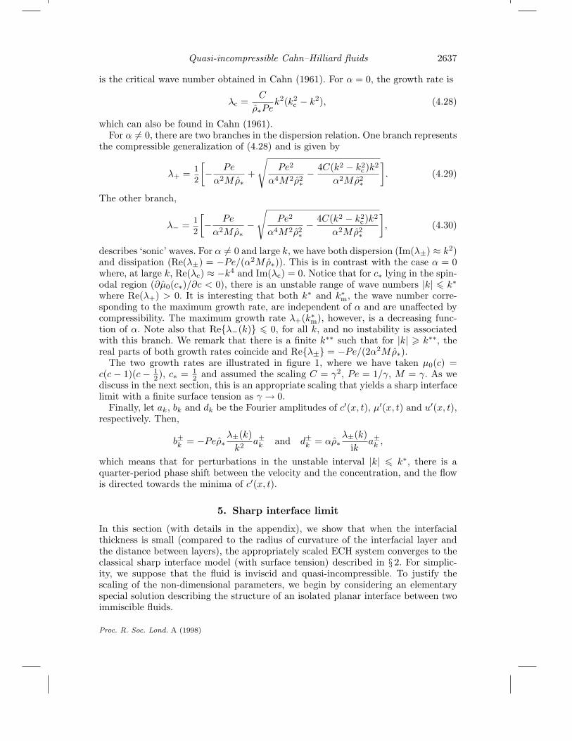
describes ‘sonic’ waves. For α 6= 0 and large k, we have both dispersion (Im(λ±) ≈ k2)and dissipation (Re(λ±) = −Pe/(α2Mρ∗)). This is in contrast with the case α = 0where, at large k, Re(λc) ≈ −k4 and Im(λc) = 0. Notice that for c∗ lying in the spin-odal region (∂µ0(c∗)/∂c < 0), there is an unstable range of wave numbers |k| 6 k∗where Re(λ+) > 0. It is interesting that both k∗ and k∗m, the wave number corre-sponding to the maximum growth rate, are independent of α and are unaffected bycompressibility. The maximum growth rate λ+(k∗m), however, is a decreasing func-tion of α. Note also that Reλ−(k) 6 0, for all k, and no instability is associatedwith this branch. We remark that there is a finite k∗∗ such that for |k| > k∗∗, thereal parts of both growth rates coincide and Reλ± = −Pe/(2α2Mρ∗).
The two growth rates are illustrated in figure 1, where we have taken µ0(c) =c(c − 1)(c − 1
2), c∗ = 12 and assumed the scaling C = γ2, Pe = 1/γ, M = γ. As we
discuss in the next section, this is an appropriate scaling that yields a sharp interfacelimit with a finite surface tension as γ → 0.
Finally, let ak, bk and dk be the Fourier amplitudes of c′(x, t), µ′(x, t) and u′(x, t),respectively. Then,
b±k = −Peρ∗λ±(k)k2 a±k and d±k = αρ∗
λ±(k)ik
a±k ,
which means that for perturbations in the unstable interval |k| 6 k∗, there is aquarter-period phase shift between the velocity and the concentration, and the flowis directed towards the minima of c′(x, t).
5. Sharp interface limit
In this section (with details in the appendix), we show that when the interfacialthickness is small (compared to the radius of curvature of the interfacial layer andthe distance between layers), the appropriately scaled ECH system converges to theclassical sharp interface model (with surface tension) described in § 2. For simplic-ity, we suppose that the fluid is inviscid and quasi-incompressible. To justify thescaling of the non-dimensional parameters, we begin by considering an elementaryspecial solution describing the structure of an isolated planar interface between twoimmiscible fluids.
Proc. R. Soc. Lond. A (1998)
2638 J. Lowengrub and L. Truskinovsky
Figure 1. Real and imaginary parts of the growth rates λ = γρ∗λ± (see (4.29) and (4.30)) asfunctions of k = γk. Close-ups of (a) Reλ±, (b) Reλ±, (c) Imλ±. The +,− indicate thecorresponding branches. The parameters are γ = 0.1 and α = 0 (solid curve); α = 2.5 (dashedcurve); and α = 5 (dot-dashed curve).
We assume that the normal to the planar layer is parallel to the z-axis and that thefluid velocity, pressure and concentration are independent of t, x and y. We furthersuppose there is no fluid velocity in the z-direction. Under these assumptions, theECH equations (4.18), (4.19) reduce to
pz + C(ρc2z)z = 0, (5.1)(df0
dc− p
ρ2
∂ρ
∂c− C
ρ(ρcz)z
)zz
= 0. (5.2)
This system is considered on the whole axis with the following boundary conditions:
c→ c± and p→ p± as z → ±∞. (5.3)
We remark that (in the inviscid case) an arbitrary z-dependent motion in the xy-plane can be superimposed. This is a consequence of the fact that in spite of thenon-hydrostatic character of the stress tensor, shear motions are decoupled from theconcentration problem.
From equation (5.1), we see that for the given concentration field c(z), the pressurep(z) can be obtained from
p(z) = p− − Cρc2z. (5.4)
To determine the concentration field, we use the Gibbs free energy
g0(c) = f0(c)− p−/ρ(c) (5.5)
Proc. R. Soc. Lond. A (1998)
Quasi-incompressible Cahn–Hilliard fluids 2639
and substitute (5.5) into equation (5.2) to obtain12Cc
2z = g0(c)− g0(c−)− µ−(c− c−). (5.6)
Here, µ− = dg0/dc|c− . In order for the boundary-value problem (5.3), (5.4) and (5.6)to have a solution, certain constraints on the limiting values (5.3) must be imposed.It is not hard to see that these constraints coincide with the classical thermodynamicconditions of equilibrium:
p+ = p−, (5.7)dg0
dc
∣∣∣∣c−
=dg0
dc
∣∣∣∣c+
, (5.8)
g0(c−)− dg0
dc
∣∣∣∣c−
c− = g0(c+)− dg0
dc
∣∣∣∣c+
c+. (5.9)
As a result, from the four constants c± and p±, only one may be chosen indepen-dently. The condition (5.7) shows that there is no pressure jump across the interfaciallayer which is a consequence of the fact that the interface is flat. In the case of sim-ple mixtures, where the density is given by (4.15), the energies g0(c) and f0(c) differby a linear function of concentration. Therefore, g0(c) can be replaced by f0(c) inequations (5.6), (5.8) and (5.9) so that (5.8) and (5.9) reduce to the Gibbs condi-tions (2.28). In the analysis that follows, we only consider simple mixtures.
We now specify the location of the interface z0 through the balance of the con-stituent mass ∫ z0
−∞(ρc− ρ−c−) dz =
∫ +∞
z0
(ρ+c+ − ρc) dz. (5.10)
Given z0, one can calculate the surface energy associated with the interfacial layer.Let σ be dimensionless excess free energy per unit area, then
σ =C
2M
∫ +∞
−∞ρc2z dz +
1M
[∫ z0
−∞ρ(c)f0(c)− ρ−f0(c−) dz
+∫ +∞
z0
ρ(c)f0(c)− ρ+f0(c+) dz], (5.11)
where we have used formula (3.36). A straightforward calculation using (5.6) and(5.11) yields
σ =C
M
∫ +∞
−∞ρc2z dz =
√2CM
∫ c+
c−ρ(c)
√√√√f0(c)− f0(c−)− df0
dc
∣∣∣∣c−
(c− c−) dc,
(5.12)
which shows that σ can be evaluated without reference to the detailed structure ofthe concentration profile. For example, if the free energy f0(c) is given by
f0(c) = 14(c− c−)2(c− c+)2, (5.13)
the coefficient of surface tension is
σ =√C
2M√
2ρ+ρ−
(c+ − c−)3
(ρ− − ρ+)2
[ρ+ + ρ− +
2ρ+ρ−ρ− − ρ+
lnρ+
ρ−
]. (5.14)
Proc. R. Soc. Lond. A (1998)
2640 J. Lowengrub and L. Truskinovsky
In this particular case, the concentration distribution c(z) and pressure distributionp(z) can also be found explicitly:
c(z) = 12(c+ + c−) + 1
2(c+ − c−) tanh[
(c+ − c−)(z − z0)2√
2C
], (5.15)
p(z) = p− − 132 ρ(c)(c+ − c−) sech4
[(c+ − c−)(z − z0)
2√
2C
]. (5.16)
Here, z0 is the position of the interface from equation (5.10).Equation (5.12) reveals that both the gradient energy term ρc2z and the bulk
chemical energy term ρf0 contribute equally to the surface energy. This is in contrastwith the situation in the level set approach (§ 1), where surface tension arises onlyfrom the gradient term (see equation (2.15)).
We now turn to the asymptotic analysis of the ECH equations in the limit when theinterfacial layers are thin and isolated. In view of equation (5.15), the sharp interfacelimit involves taking C → 0. Also, equation (5.12) shows that in order to have afinite surface tension coefficient in this limit, the generalized Mach number mustsatisfy M ∼ √C. Therefore, it is natural to introduce a small parameter γ =
√C as
a measure of the thickness of the interface, and to assume the scaling M = γ. Thisessentially fixes the coefficient of surface tension. We also take Pe = 1/γ, which meansthat diffusion is assumed to be slow. The scaling of M implies that the characteristicvelocity V∗ √µ∗, while the scaling of Pe is equivalent to the following restrictionon the mobility ν ρ∗L∗/
√µ∗. Similar scaling has recently been used by Gurtin et
al . (1996) and Golovaty (1996) in the framework of model H. We remark that thesharp interface limit can also be obtained by using the assumption of faster diffusion,say Pe = 1 (cf. Starovoitov 1994).
Using the above scaling (and Re =∞), we rewrite the ECH system as
div v = −1ρ
(∂ρ
∂c
)c, (5.17)
ρv = −(1/γ)[∇p+ γ2 div(ρ∇c⊗∇c)], (5.18)ρc = γ∇µ, (5.19)
where
µ =df0
dc− p
ρ2
∂ρ
∂c− γ2
ρdiv(ρ∇c). (5.20)
We show in the appendix that this system, in the case of an isolated transition layer,is compatible with the sharp interface incompressible Euler model in the limit γ → 0.
6. Example of a topological transition
If the curvature of the transition layer is large, e.g. κ = O(1/√C), then the asymp-
totic analysis presented in the previous section breaks down. For this type of transi-tion layer, the NSCH system behaves differently from the sharp interface model. Forexample, in the sharp interface model for inviscid fluids, the Laplace formula saysthat the pressure diverges at large curvatures, which is typical near a topological tran-sition. In the NSCH model, the effective surface tension varies with curvature , whichmollifies this divergence. To demonstrate this effect, we consider a simple example
Proc. R. Soc. Lond. A (1998)
Quasi-incompressible Cahn–Hilliard fluids 2641
of a topological transition: the annihilation (nucleation) of a spherical droplet of onefluid immersed in an infinite reservoir of another fluid. The simplicity of the geome-try allows us to investigate the fine structure of the diffuse interface when the radiusof the drop is O(
√C).
Suppose that there is no fluid motion, and consider stationary solutions of thequasi-incompressible NSCH system (4.18), (4.19) with spherical symmetry. Theresulting system of ordinary differential equations is
pr + (C/r2)(ρr2c2r)r = 0, (6.1)r2[
df0
dc− p
ρ2
∂ρ
∂c− C
ρr2 (ρr2cr)r
]r
r
= 0, (6.2)
which is analogous to the system (5.1), (5.2) for the planar interface. The boundaryconditions are given by
limr→∞ c(r) = c∞ and lim
r→∞ p(r) = p∞. (6.3)
Symmetry considerations also require that cr → 0 as r → 0. Contrary to the planarcase, the constants c∞ and p∞ can be chosen independently as we shall see below.While equations (6.1) and (6.2) always have a trivial homogeneous solution c(r) = c∞and p(r) = p∞, we seek non-trivial solutions in which the concentration is a monotonefunction of r. By varying c∞, or by varying the mass of the constituent, we can varythe size of the droplet. The corresponding sequence of equilibrium states may alsobe interpreted as describing a quasi-steady evolution.
As in the planar case, equations (6.1) and (6.2) can be decoupled. If the densities ofthe fluids are not matched (i.e. dρ/dc 6= 0), we obtain an integro-differential equationfor the concentration field. In fact, equation (6.1) can be integrated to yield
p = p∞ − Cρc2r + 2C∫ ∞r
ρc2rr
dr, (6.4)
while equation (6.2) can be transformed to
−12Cc
2r = f0(c)− [f0(c∞) + µ∞(c− c∞)] +
(p
ρ− p∞ρ∞
), (6.5)
where µ∞ = df0/dc(c∞) and ρ∞ = ρ(c∞). From equations (6.4) and (6.5), we obtainthe following necessary conditions for the existence of a non-trivial solution:
p0 = p∞ + 2C∫ ∞
0ρc2rr
dr, (6.6)
f0(c0)− [f0(c∞) + µ∞(c0 − c∞)] +(p0
ρ0− p∞ρ∞
)= 0, (6.7)
where p0 = p(0), c0 = c(0) and ρ0 = ρ(c0). These conditions are analogous to condi-tions (5.7)–(5.9) in the planar case. Since there are only two equations for the fourunknowns, c0, c∞, p0 and p∞, we see that c∞ and p∞ can be chosen independentlyof each other.
In order to compare the diffuse fluid drop with a sharp interface drop, we introducean effective radius through the mass balance condition (analogous to equation (5.10)defining z0 in the planar case). For simplicity, we suppose that the density is given
Proc. R. Soc. Lond. A (1998)
2642 J. Lowengrub and L. Truskinovsky
by the simple mixture formula (4.15). The effective radius of the diffuse drop, R0, isimplicitly given by the following condition:∫ R0
0[ρ(c)c− ρ(c0)c0]r2 dr =
∫ ∞R0
[ρ(c∞)c∞ − ρ(c)c]r2 dr. (6.8)
Since the drop’s surface is diffuse, this choice of an effective radius is obviously notunique. Using this value R0, we can define the excess surface energy per unit areaby the formula
σ∗ =1
MR20
12C
∫ ∞0
ρc2rr2 dr +
∫ R0
0[ρ(c)f0(c)− ρ(c0)f0(c0)]r2 dr
+∫ ∞R0
[ρ(c)f0(c)− ρ(c∞)f0(c∞)]r2 dr, (6.9)
which is analogous to (5.11) in the planar interface case. Contrary to the planarcase, however, σ∗ cannot be evaluated without first computing the full concentrationprofile c(r). We can simplify (6.9), though, to obtain
σ∗ =C
M
∫ ∞0
c2r
[r2
3R20
+2R0
3r
]ρ dr. (6.10)
An alternative definition for the coefficient of surface tension can be obtained bygeneralizing the Laplace formula and writing
p0 = p∞ + 2(σ∗∗/R0)M, (6.11)
which defines σ∗∗. Using equation (6.6), we obtain
σ∗∗ =C
M
∫ ∞0
c2rR0
rρ dr. (6.12)
We notice that the expressions for both σ∗ and σ∗∗ depend explicitly on the effectiveradius of curvature R0. To determine R0, we first obtain the concentration profile bysolving equations (6.4) and (6.5), and then use equation (6.8) to obtain
R0 = R0(c∞) =
3∫ ∞
0
[ρ(c)c− ρ(c∞)c∞ρ(c0)c0 − ρ(c∞)c∞
]r2 dr
1/3
. (6.13)
Following Cahn & Hilliard (1959), we can analyse the behaviour of R0, σ∗ and σ∗∗in certain limiting cases, without computing the concentration and pressure profiles.For example, in the limit when c∞ approaches the planar equilibrium concentra-tion c− from above, we get limc∞→c− c0 = c+ and limc∞→c− p0 = p∞, where c+is the other equilibrium concentration for the planar interface. One can see thatthere is no pressure jump across the diffuse interface in this limit. We further obtainlimc∞→c− σ
∗ = limc∞→c− σ∗∗ = σ, where σ is the surface energy for the planar inter-
face given in equation (5.12). Therefore, the different definitions of surface tensionagree in this limit. Also,
limc∞→c−
(c∞ − c−)R0(c∞) =2σMρ+
(d2f0
dc2(c+)
)−1
,
which shows how the effective radius R0 diverges in the vicinity of the planar equi-librium concentration.
Proc. R. Soc. Lond. A (1998)
Quasi-incompressible Cahn–Hilliard fluids 2643
Another limiting case occurs when c∞ = cs; here, cs is a spinodal point whered2f0/d2c changes sign. In this limit, the solution of (6.4) and (6.5) converges to thetrivial homogeneous state c(r) = c∞ and p(r) = p∞. We remark that the energydifference between the non-trivial and the trivial solutions is finite for c− < c∞ < csand tends to zero as c∞ → cs.
To illustrate these limits, as well as the behaviour of the solution in the interme-diate range of concentrations, we shall first consider the case where the fluids aredensity matched and equation (6.2) reduces to the radial Cahn–Hilliard equation,
C
(crr +
2rcr
)=
ddc
(f0(c)− µ∞c). (6.14)
This semilinear equation has been studied extensively by many authors (see, forexample, Truskinovsky 1983; Dell’Isola et al . 1998). Here, we obtain a new explicitsolution by considering a piecewise quadratic free energy f0(c). In this special case,the problem reduces to a system of nonlinear algebraic equations.
The simplest smooth piecewise quadratic function, containing a non-trivial spin-odal region, consists of three parabolas:
f0(c) =
14c
2, c 6 16 ,
18 [ 1
16 − (c− 12)2], 1
6 < c < 56 ,
14(c− 1)2, c > 5
6 .
(6.15)
Using the energy (6.15), it is straightforward to calculate the solution of equa-tion (6.14) analytically. We obtain three linear equations for c corresponding to eachof the three parabolas. We then patch the solution together, insuring the continuityof c and cr. We find that for c∞ ∈ (0, 1
6) and c∞ ∈ (56 , 1), there is a unique monotone
solution c(r). The solutions are parametrized by c∞ and depend on R1 and R2, thecoordinates of the points in r where the parabolas are switched.
After a simple calculation, we obtain
c(r) =
(B/r)e−r/
√2 + c∞, r > R1,
12 − 2c∞ − (1/r)[C cos(1
2r) +D sin(12r)], R2 < r < R1,
1 + c∞ + (A/r)(er/√
2 − e−r/√
2), r 6 R2,
(6.16)
where, on the right-hand side, the spatial variable is normalized by√C. In the analy-
sis that follows, we use the normalized variables r/√C and Ri/
√C. The coefficients
A, B, C and D can be given in terms of R1 and R2, which satisfy the followingnonlinear system of algebraic equations:
−β(
1√2
+3R1
)= β cot 1
2(R2 −R1) +R2
R1csc 1
2(R2 −R1),
3R2− 1√
2coth
R2√2
= βR1
R2csc 1
2(R2 −R1) + cot 12(R2 −R1).
Here, β = (16 − c∞)/(1
6 + c∞). We note that there is a critical value c∞ = c∗∞ atwhich R2 = 0. When R2 = 0, the solution is given by
c(r) =
(B/r)e−r/
√2 + c∞, r > R∗1,
12 − 2c∞ − (D/r) sin(1
2r), 0 6 r < R∗1,(6.17)
Proc. R. Soc. Lond. A (1998)
2644 J. Lowengrub and L. Truskinovsky
Figure 2. Concentration profiles describing spherical droplets with c∞ = 0.035, 0.10 and 0.15.The dotted curves correspond to the free energy (6.15), while the solid curves correspond thefree energy (6.20). The radius is scaled as r = r/
√C.
where the coefficients B and D can again be expressed in terms of R∗1 and
tan(12R∗1) =
R∗1√
2R∗1 + 3
√2. (6.18)
The critical value c∗∞ is given in terms of R∗1 by
c∗∞ =R∗1 + 2 sin(1
2R∗1)
6(R∗1 − 2 sin(12R∗1))
. (6.19)
From (6.18) and (6.19), we obtain R∗1 ∼= 7.764 and c∗∞ ∼= 0.117. For c∞ ∈ (c∗∞,16), we
also have R2 = 0 and R1 = R∗1, so the non-trivial monotone solution never reachesthe third parabola.
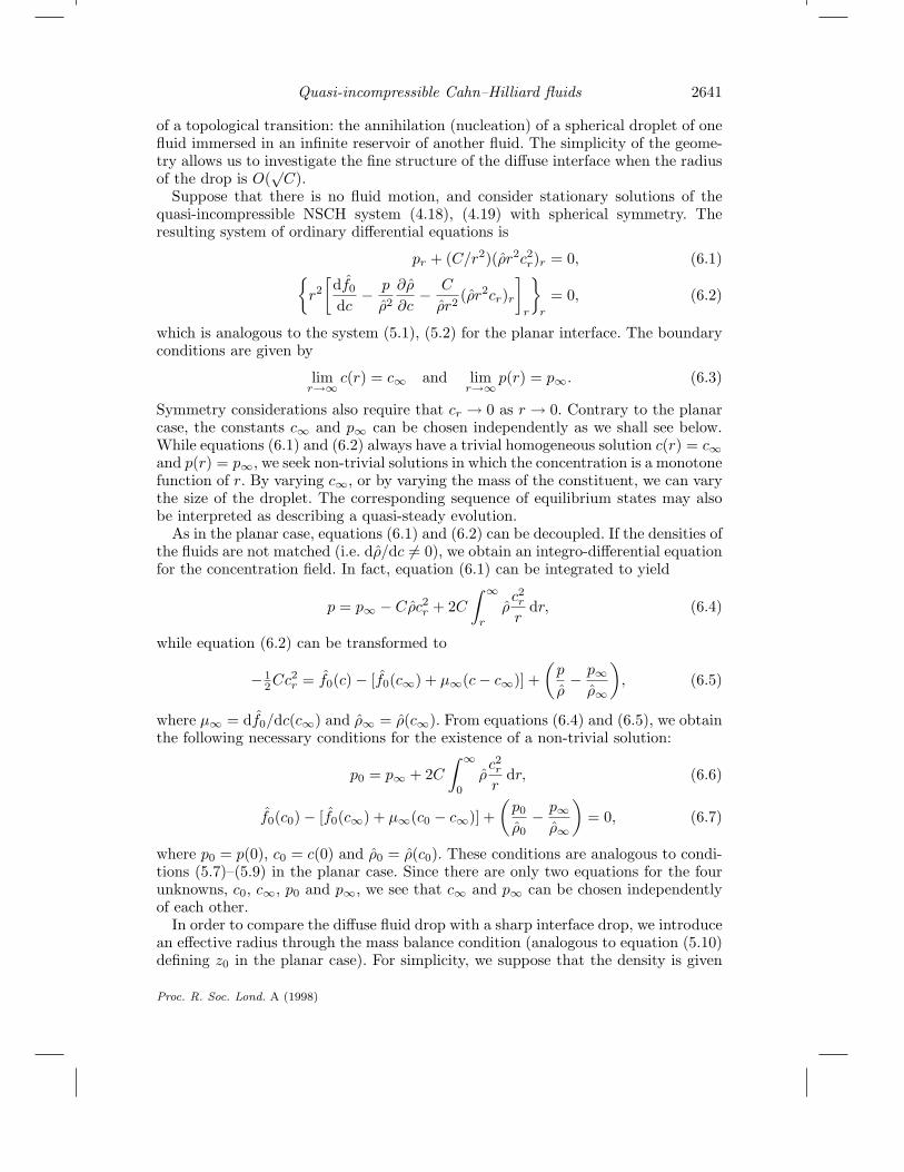
The qualitative change in structure of the solution across c∞ = c∗∞ can be viewedas a sign of the beginning of the topological transition. In fact, we can interpret R2and R1 as defining the inner and outer boundaries of the diffuse droplet interface.After the inner boundaryR2 vanishes, the second fluid region disappears and the dropconsists entirely of the interfacial region. At larger values of c∞, the interfacial regionalso disappears, which marks the completion of the transition. Since no singularitiesdevelop, we conclude that the CH model provides a smooth description of this simpletopological change. In figure 2, the concentration profiles are shown, as functions ofthe normalized radius r/
√C, for three different values of c∞.
In order to show that the approximation of the energy function by three parabolasis robust, we compare our analytic solution with the results of a direct numericalintegration of (6.14) by using the fourth-order polynomial energy
f0(c) = 14c
2(c− 1)2, (6.20)
Proc. R. Soc. Lond. A (1998)
Quasi-incompressible Cahn–Hilliard fluids 2645
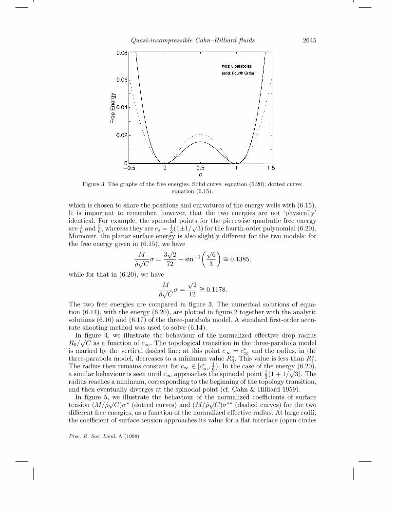
Figure 3. The graphs of the free energies. Solid curve: equation (6.20); dotted curve:equation (6.15).
which is chosen to share the positions and curvatures of the energy wells with (6.15).It is important to remember, however, that the two energies are not ‘physically’identical. For example, the spinodal points for the piecewise quadratic free energyare 1
6 and 56 , whereas they are cs = 1
2(1±1/√
3) for the fourth-order polynomial (6.20).Moreover, the planar surface energy is also slightly different for the two models: forthe free energy given in (6.15), we have
M
ρ√Cσ =
3√
272
+ sin−1(√
63
)∼= 0.1385,
while for that in (6.20), we have
M
ρ√Cσ =
√2
12∼= 0.1178.
The two free energies are compared in figure 3. The numerical solutions of equa-tion (6.14), with the energy (6.20), are plotted in figure 2 together with the analyticsolutions (6.16) and (6.17) of the three-parabola model. A standard first-order accu-rate shooting method was used to solve (6.14).
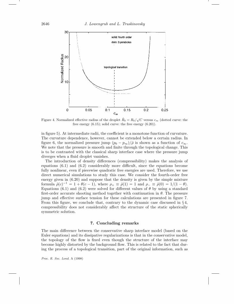
In figure 4, we illustrate the behaviour of the normalized effective drop radiusR0/√C as a function of c∞. The topological transition in the three-parabola model
is marked by the vertical dashed line: at this point c∞ = c∗∞ and the radius, in thethree-parabola model, decreases to a minimum value R∗0. This value is less than R∗1.The radius then remains constant for c∞ ∈ [c∗∞,
16). In the case of the energy (6.20),
a similar behaviour is seen until c∞ approaches the spinodal point 12(1 + 1/
√3). The
radius reaches a minimum, corresponding to the beginning of the topology transition,and then eventually diverges at the spinodal point (cf. Cahn & Hilliard 1959).
In figure 5, we illustrate the behaviour of the normalized coefficients of surfacetension (M/ρ
√C)σ∗ (dotted curves) and (M/ρ
√C)σ∗∗ (dashed curves) for the two
different free energies, as a function of the normalized effective radius. At large radii,the coefficient of surface tension approaches its value for a flat interface (open circles
Proc. R. Soc. Lond. A (1998)
2646 J. Lowengrub and L. Truskinovsky
Figure 4. Normalized effective radius of the droplet R0 = R0/√C versus c∞ (dotted curve: the
free energy (6.15); solid curve: the free energy (6.20)).
in figure 5). At intermediate radii, the coefficient is a monotone function of curvature.The curvature dependence, however, cannot be extended below a certain radius. Infigure 6, the normalized pressure jump (p0 − p∞)/ρ is shown as a function of c∞.We note that the pressure is smooth and finite through the topological change. Thisis to be contrasted with the classical sharp interface case where the pressure jumpdiverges when a fluid droplet vanishes.
The introduction of density differences (compressibility) makes the analysis ofequations (6.1) and (6.2) considerably more difficult, since the equations becomefully nonlinear, even if piecewise quadratic free energies are used. Therefore, we usedirect numerical simulations to study this case. We consider the fourth-order freeenergy given in (6.20) and suppose that the density is given by the simple mixtureformula ρ(c)−1 = 1 + θ(c − 1), where ρ+ ≡ ρ(1) = 1 and ρ− ≡ ρ(0) = 1/(1 − θ).Equations (6.1) and (6.2) were solved for different values of θ by using a standardfirst-order accurate shooting method together with continuation in θ. The pressurejump and effective surface tension for these calculations are presented in figure 7.From this figure, we conclude that, contrary to the dynamic case discussed in § 4,compressibility does not considerably affect the structure of the static sphericallysymmetric solution.
7. Concluding remarks
The main difference between the conservative sharp interface model (based on theEuler equations) and its dissipative regularizations is that in the conservative model,the topology of the flow is fixed even though the structure of the interface maybecome highly distorted by the background flow. This is related to the fact that dur-ing the process of a topological transition, part of the original information, such as
Proc. R. Soc. Lond. A (1998)
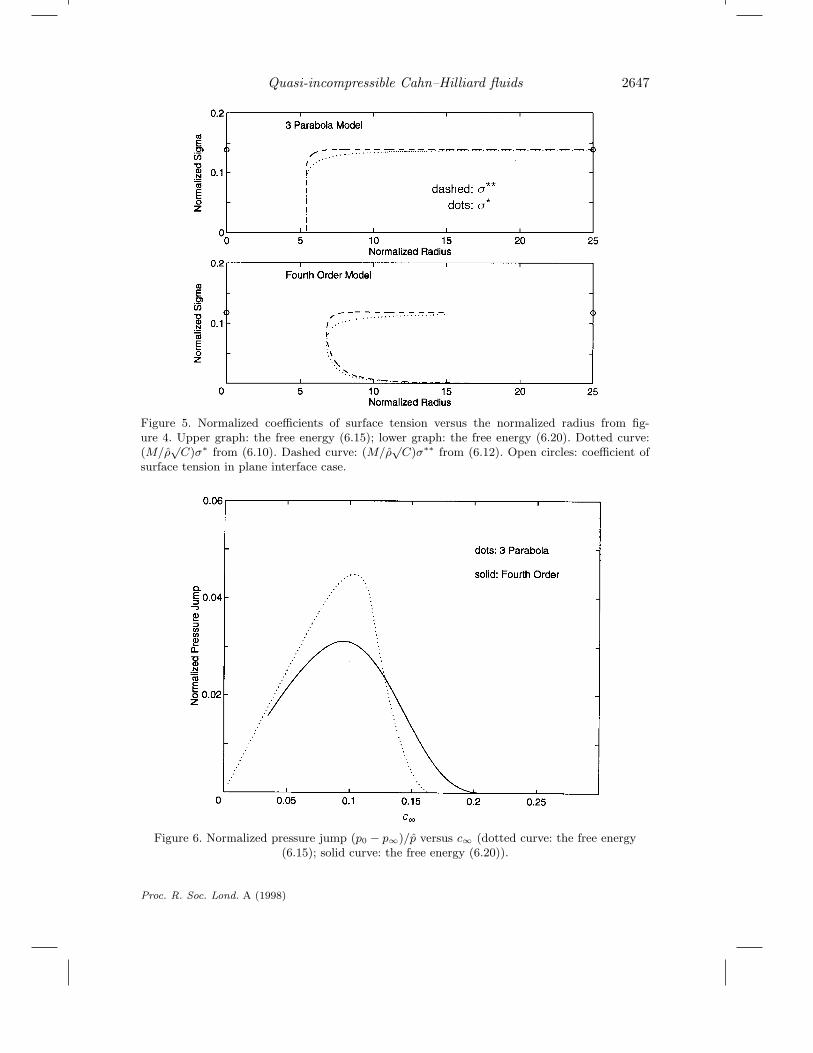
Quasi-incompressible Cahn–Hilliard fluids 2647
Figure 5. Normalized coefficients of surface tension versus the normalized radius from fig-ure 4. Upper graph: the free energy (6.15); lower graph: the free energy (6.20). Dotted curve:(M/ρ
√C)σ∗ from (6.10). Dashed curve: (M/ρ
√C)σ∗∗ from (6.12). Open circles: coefficient of
surface tension in plane interface case.
Figure 6. Normalized pressure jump (p0 − p∞)/p versus c∞ (dotted curve: the free energy(6.15); solid curve: the free energy (6.20)).
Proc. R. Soc. Lond. A (1998)
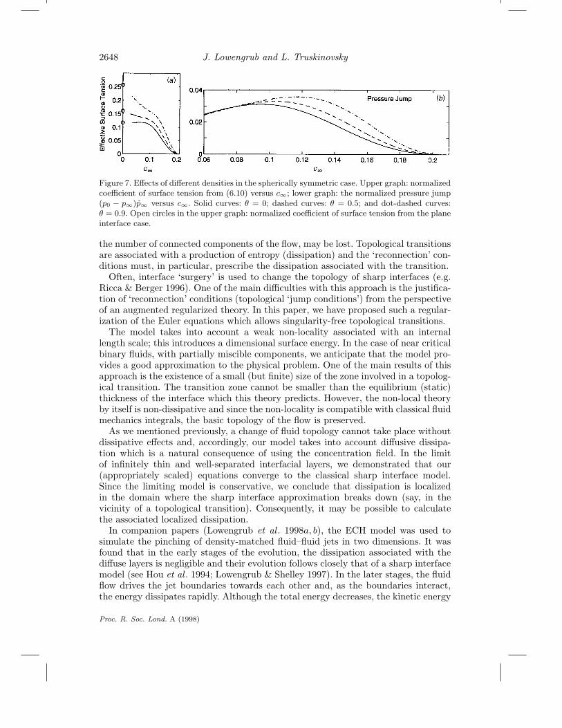
2648 J. Lowengrub and L. Truskinovsky
Figure 7. Effects of different densities in the spherically symmetric case. Upper graph: normalizedcoefficient of surface tension from (6.10) versus c∞; lower graph: the normalized pressure jump(p0 − p∞)p∞ versus c∞. Solid curves: θ = 0; dashed curves: θ = 0.5; and dot-dashed curves:θ = 0.9. Open circles in the upper graph: normalized coefficient of surface tension from the planeinterface case.
the number of connected components of the flow, may be lost. Topological transitionsare associated with a production of entropy (dissipation) and the ‘reconnection’ con-ditions must, in particular, prescribe the dissipation associated with the transition.
Often, interface ‘surgery’ is used to change the topology of sharp interfaces (e.g.Ricca & Berger 1996). One of the main difficulties with this approach is the justifica-tion of ‘reconnection’ conditions (topological ‘jump conditions’) from the perspectiveof an augmented regularized theory. In this paper, we have proposed such a regular-ization of the Euler equations which allows singularity-free topological transitions.
The model takes into account a weak non-locality associated with an internallength scale; this introduces a dimensional surface energy. In the case of near criticalbinary fluids, with partially miscible components, we anticipate that the model pro-vides a good approximation to the physical problem. One of the main results of thisapproach is the existence of a small (but finite) size of the zone involved in a topolog-ical transition. The transition zone cannot be smaller than the equilibrium (static)thickness of the interface which this theory predicts. However, the non-local theoryby itself is non-dissipative and since the non-locality is compatible with classical fluidmechanics integrals, the basic topology of the flow is preserved.
As we mentioned previously, a change of fluid topology cannot take place withoutdissipative effects and, accordingly, our model takes into account diffusive dissipa-tion which is a natural consequence of using the concentration field. In the limitof infinitely thin and well-separated interfacial layers, we demonstrated that our(appropriately scaled) equations converge to the classical sharp interface model.Since the limiting model is conservative, we conclude that dissipation is localizedin the domain where the sharp interface approximation breaks down (say, in thevicinity of a topological transition). Consequently, it may be possible to calculatethe associated localized dissipation.
In companion papers (Lowengrub et al . 1998a, b), the ECH model was used tosimulate the pinching of density-matched fluid–fluid jets in two dimensions. It wasfound that in the early stages of the evolution, the dissipation associated with thediffuse layers is negligible and their evolution follows closely that of a sharp interfacemodel (see Hou et al . 1994; Lowengrub & Shelley 1997). In the later stages, the fluidflow drives the jet boundaries towards each other and, as the boundaries interact,the energy dissipates rapidly. Although the total energy decreases, the kinetic energy
Proc. R. Soc. Lond. A (1998)
Quasi-incompressible Cahn–Hilliard fluids 2649
of the fluid increases through the production of vorticity. The calculation capturesthe topology transition from a two-dimensional jet to a system of fluid droplets.
It was also found that the limiting step in these computations is the resolutionof the fluid motion, rather than the structure of the concentration field, and thatin order for the concentration boundary layers to be resolved, their thickness needsto be at least several grid lengths. Since the simulations using the ECH model aregenerically much more expensive than those based on the boundary integral method,it is natural to conclude that the ideal numerical approach should be based on thesharp interface model and then use ‘jump conditions’ to transit the sharp interfacethrough a topology change.
We view the study of the annihilation of a spherical droplet as a first step inestablishing justified ‘cut and connect’ procedures. In particular, we have shownthat the extra energy associated with the nucleus is finite, which effectively fixesthe value of dissipation associated with the topological transition. Presently, it isnot clear whether such a separation of scales can always be done since the topologychange may, in principle, produce fluid fragments that cannot be described within asharp interface model.We thank J. Goodman, D. Joseph, P. Leo, G. Lopez, G. McFadden, M. Shelley and Y. Shikhmur-zaev for important comments and Elizabeth Lowengrub for proof-reading the manuscript. J.L.acknowledges support from the NSF grant DMS-940310, the Sloan foundation, the McKnightfoundation and the Minnesota Supercomputer Institute; L.T. acknowledges support from theNSF grant DMS-9501433 and the Minnesota Supercomputer Institute.
Appendix A. Matched asymptotic expansions
Here we use the method of matched asymptotic expansions to show that the system(5.17)–(5.20) formally converges as γ → 0 to the incompressible Euler equationswith a sharp interface. In order for our expansions to be valid, the curvature κ ofthe layer must satisfy κ 1/γ and the multiple layers must be separated by adistance which is at least O(1). Following the standard approach (see, for example,Pego 1989), we suppose that at time t = 0, there is a single smooth transition layerof width O(γ). The initial concentration is assumed to be c(x, 0) = c± + O(γ) inΩ±, where c± are equilibrium concentrations which satisfy the conditions (5.7)–(5.9)for some p±. These initial conditions are consistent with the experiments on theKelvin–Helmholtz instability performed by Thorpe (1969), where two different fluidswere allowed to equilibrate before gravity-induced motion was impulsively started.We further suppose that the most rapid variation in the velocity field for t > 0 takesplace across the concentration transition layer. This is consistent with assumingthat the fluid motion occurs on faster time-scale than the chemical diffusion (ourassumption Pe 1).
Suppose that in the domains Ω± (outer region), far from the transition layer, thevelocity, concentration and pressure fields can be given in terms of a regular expansionin the small parameter γ, i.e. A(x, t) = A(0)(x, t)+γA(0)(x, t)+· · · , where A(x, t) is ageneric variable. Using these expansions in the equations (5.17)–(5.20) and matchingpowers of γ, we obtain
∇p(0) = 0at O(1/γ), while at O(1), we obtain
div v(0) = 0,
Proc. R. Soc. Lond. A (1998)
2650 J. Lowengrub and L. Truskinovsky
ρ(c(0))(v(0)t + v(0) · ∇v(0)) = −∇p(1),
c(0)t + v(0) · ∇c(0) = 0,
which are the classical Euler equations.Near the transition layer (inner region), we choose φ(x, t) to be the signed distance
function from a point x to the limiting sharp interfacial surface Σ(t) and introducethe stretched normal coordinate z = φ(x, t)/γ. Then, Σ(t) has unit normal n = ∇φ,normal velocity D = −φ, and mean curvature 2κ = −∇2φ. In the inner region, wesuppose the following generic expansion holds:
A(x, t) = A(0)(z, x, t) + γA(1)(z, x, t) + · · · ,where x(x, t) are two coordinates on the surface φ(x, t) = 0. We use these expansionsin equations (5.17)–(5.20), together with the change of variable formulae
∇ =1γn∂z +∇x, ∇2 =
1γ2 ∂zz −
2κγ∂z +∇2
x and dt = −Dγ∂z + ∂t.
From the normal component of equation (5.18), we obtain at O(1/γ2)
p(0)z + (ρ(c(0))(c(0)
z )2)z = 0.
At O(1/γ), we obtain:
u(0)z =
ρ′(c(0))ρ(c(0))
(u(0) −D)c(0)z
from equation (5.17);
ρ(c(0))(u(0) −D)u(0)z = −p(1)
z − 2κρ(c(0))(c(0)z )2
+ [2ρ(c(0))c(0)z c(1)
z + ρ′(c(0))(c(0)z )2(3c(1) − 2c(1)
z )]zfrom the normal component of equation (5.18);
ρ(c(0))(u(0) −D)w(0)z = −[∇xp(0) + (ρ′(c(0))(c(0)
z )2
+ ρ(c(0))c(0)zz )∇xc(0) + 1
2 ρ(c(0))∇x(c(0))2]
from the tangential components of equation (5.18); and finally,
ρ(c(0))(u(0) −D)c(0)z =
[µ0(c(0))− ρ′(c(0))
ρ(c(0))p(0) − 1
ρ(c(0))(ρ(c(0))c(0)
z )z
]zz
from equations (5.19) and (5.20). In the above, u(0) = v(0) · n and w(0) = v(0) −(v(0) · n)n. We note that if the curvature κ = O(1/γ), then the local coordinatesystem near Σ typically becomes singular and the ordering of the above expansionsbreaks down.
To match the inner and outer expansions, we suppose that the outer expansionholds up to the surface Σ. Then, near Σ, we expand the outer solution in the innervariables and match each power of γ with the limiting values of the inner solution.For example,
limz→±∞ A
(0)(z, x, t) = A(0)(x, t)±, limz→±∞ A
(1)(z, x, t) = A(1)(x, t)±
limz→±∞ A
(1)z (z, x, t) = n · ∇A(0)(x, t)±,
Proc. R. Soc. Lond. A (1998)
Quasi-incompressible Cahn–Hilliard fluids 2651
where the ± denotes the limiting values on Σ from Ω±.At O(1/γ) in the outer expansion, we obtain
p(0)(x, t) = p± = const. in Ω±,
although the constant could take different values in each region. From the innerexpansion at O(1/γ2), we obtain
p(0)(z, x, t) = p− − ρ(c(0))(c(0)z )2 and p− = p+,
which means that (in the leading order) the outer pressure is a global constant.At O(1/γ) in the inner expansion, we obtain
u(0)(z, x, t) = D(x, t),
which, together for the matching condition for velocity, shows that
[[v(0) · n]]Σ = 0 and v(0) · n = D.
Consequently, the interface moves with the fluid at the outer scale. In addition, fromthe inner expansion, we obtain
c(0)(z, x, t) = C(z + α(x, t)),
where C(z) is the unique planar interface, described in § 5, with C(0) = 12(c+ + c−).
The function α(x, t) is an arbitrary translation; this can be set to zero by using acentring condition of the type given in Pego (1989) which links the position of theinterfacial surface Σ with the inner expansion. Using the matching condition for theconcentration and the initial condition for the concentration, we obtain
c(0)(x, t) = c± in Ω±.
Then from the inner expansion, we get
p(1)z = 2κρ(c(0))(c(0)
z )2 + [2ρ(c(0))c(0)z c(1)
z + ρ′(c(0))(c(0)z )2(3c(1) − 2c(1)
z )]z.
Using the first-order matching condition for pressure, we conclude that
[[p(1)]]Σ = 2κ∫ +∞
−∞ρ(C)C2
z dz,
which shows that the jump in the outer pressure p(1) across Σ is proportional tothe mean curvature of Σ. We note that the integral in the right-hand side of thisformula is exactly the one which appeared in equation (5.12), divided by γ. Finally,we note that equation for the tangential components of linear momentum is triviallysatisfied so that the tangential velocity w(0) does not appear at this order. Thus, inthe leading order, the jump of the outer tangential velocity (across Σ) is arbitrary.
These results show that the limiting sharp interface moves with the fluid, the Eulerequations hold on each side of the interface and the Laplace condition is satisfiedwith the surface tension given by equation (5.12). We also notice that the energy(3.36) converges, as γ → 0, to the expression
E(t) = 12ρ+
∫Ω+
|v(0)|2 d3x+ 12ρ−
∫Ω−|v(0)|2 d3x+ σ|Σ(t)|,
which is the energy of the sharp interface model. Here, for simplicity, we assumedf0(c±) = f ′0(c±) = 0.
Proc. R. Soc. Lond. A (1998)
2652 J. Lowengrub and L. Truskinovsky
References
Aifantis, E. C. & Serrin, J. B. 1983 The mechanical theory of fluid interfaces and Maxwell’srule. J. Coll. Int. Sci. 96, 517–529.
Anderson, D. M. & McFadden, G. B. 1997 A diffuse-interface description of internal waves innear critical fluid. Phys. Fluids A 9, 1870–1879.
Antanovskii, L. 1995 A phase field model of capillarity. Phys. Fluids A 7, 747–753.Atkin, R. J. & Crane, R. E. 1976 Continuum theories of mixtures: basic theory and historical
development. Q. J. Mech. Appl. Math. 29, 209–244.Bedford, A. & Drumheller, D. S. 1983 Theories of immiscible and structured mixtures. Int. J.
Engng Sci. 21, 863–960.Brackbill, J. U., Kothe, D. B. & Zemach, C. 1994 A continuum method for modelling surface
tension. J. Comp. Phys. 100, 335–354.Cahn, J. W. 1961 On spinodal decomposition. Acta Metall. 9, 795–801.Cahn, J. W. & Hilliard, J. E. 1958 Free energy of non-uniform system. I. Interfacial free energy.
J. Chem. Phys. 28, 258–267.Cahn, J. W. & Hilliard, J. E. 1959 Free energy of non-uniform system. III. J. Chem. Phys. 31,
688–699.Chang, Y. C., Hou, T. Y., Merriman, B. & Osher, S. 1996 A level set formulation of Eulerian
interface capturing methods for incompressible fluid flows. J. Comp. Phys. 124, 449–464.Chella, R. & Vinals, J. 1996 Mixing of a two-phase fluid by cavity flow. Phys. Rev. E 53, 3832–
3840.Davis, H. T. & Scriven, L. E. 1982 Stress and structure in fluid interfaces. Adv. Chem. Phys.
49, 57–454.Davydov, B. 1949 Variational principles and canonical equations for ideal fluid. Dokl. Akad.
Nauk SSSR 69, 165–168.Dell’Isola, F., Gouin, H. & Rotoli, G. 1998 Nucleation of spherical shell-like interfaces by second
gradient theory: numerical simulations. Eur. J. Mech. Fluids (In the press.)Eggers, J. 1995 Theory of drop formation. Phys. Fluids 7, 941–953.Eggers, J. & Dupont, T. F. 1994 Drop formation in a one-dimensional approximation of the
Navier–Stokes equations. J. Fluid Mech. 262, 205.Elliot, C. M. 1989 The Cahn–Hilliard model for the kinetics of phase separation. In Mathematical
models for phase change problems (ed. J. F. Rodrigues). International Series in NumericalMathematics, vol. 88, pp. 35. Basel: Birkhauser.
Ericksen, J. L. 1991 Liquid crystals with variable degree of orientation. Arch. Ration. Mech.Analysis 113, 97–120.
Falk, F. 1992 Cahn–Hilliard theory and irreversible thermodynamics. J. Non-Equilib. Thermo-dyn. 17, 53–65.
Galdi, P., Joseph, D. D., Preziosi, L. & Rionero, S. 1991 Mathematical problems for miscible,incompressible fluids with Korteweg stresses. Eur. J. Mech. Fluids 10, 253–267.
Gibbs, J. 1875a On the equilibrium of heterogeneous substances. Trans. Connect. Acad. 111,108–248
Gibbs, J. 1875b On the equilibrium of heterogeneous substances. Trans. Connect. Acad. 111,343–524.
Golovaty, D. 1996 On the asymptotic behaviour of the equations describing the motion of anincompressible binary fluid. (Preprint.)
Gurtin, M. 1989 On a non-equilibrium thermodynamics of capillarity and phase. Q. Appl. Math.47, 129–145.
Gurtin, M. E. & McFadden, G. B. (eds) 1992 On the evolution of phase boundaries. IMA Seriesin Mathematics and its Applications, no. 43. Springer.
Proc. R. Soc. Lond. A (1998)
Quasi-incompressible Cahn–Hilliard fluids 2653
Gurtin, M. E., Polignone, D. & Vinals, J. 1996 Two-phase binary fluids and immiscible fluidsdescribed by an order parameter. Math. Models Meth. Appl. Sci. 6, 815–831.
Hohenberg, P. C. & Halperin, B. I. 1977 Theory of dynamic critical phenomena. Rev. Mod.Phys. 49, 435–479.
Hou, T. Y., Lowengrub, J. S. & Shelley, M. J. 1994 Removing the stiffness from interfacial flowswith surface tension. J. Comp. Phys. 114, 312–338.
Hou, T. Y., Lowengrub, J. S. & Shelley, M. J. 1997 The long-time motion of vortex sheets withsurface tension. Phys. Fluids A 9, 1933–1954.
Jacqmin, D. 1998 Contact line dynamics of a diffuse fluid interface. Phys. Fluids A. (Submitted.)Jasnow, D. & Vinals, J. 1996 Coarse-grained description of thermo-capillary flow. Phys. Fluids
A 8, 660–669.Joseph, D. D. 1990 Fluid dynamics of two miscible liquids with diffusion and gradient stresses.
Eur. J. Mech. Fluids 9, 565–596.Joseph, D. D. & Rennardy, Y. Y. 1993 Fundamentals of two fluid mechanics. Springer.Keller, J. B. & Merchant, G. J. 1991 Flexural rigidity of a liquid surface. J. Stat. Phys. 63,
1039–1051.Keller, J. B. & Miksis, M. 1983 Surface tension driven flows. SIAM J. Appl. Math. 43, 268–277.Kikuchi, R. & Cahn, J. W. 1962 Theory of domain walls in ordered structures. II. Pair approx-
imations for non-zero temperatures. J. Phys. Chem. Solids 23, 137–151.Koga, T. E. & Kawasaki, K. 1991 Spinodal decomposition in binary fluids: effects of hydrody-
namic interactions. Phys. Rev. A 44(2), R817–R820.Lamb, H. 1945 Hydrodynamics. New York: Dover.Landau, L. D. & Lifshitz, E. M. 1958 Statistical physics. Oxford: Pergamon.Landau, L. D. & Lifshitz, E. M. 1959 Fluid mechanics. Oxford: Pergamon.Lowengrub, J. S., Shelley, M. J., Truskinovsky, L. & Goodman, J. 1998a The break-up of liquid
jets in Cahn–Hilliard hydrodynamics. (In preparation.)Lowengrub, J. S., Goodman, J., Lee, H., Longmire, E., Shelley, M. & Truskinovsky, L. 1998b
Topological transitions in liquid/liquid interfaces. In Proc. 1997 Int. Conf. on Free BoundaryProblems, Crete. (In the press.)
Mansour, N. & Lundgren, T. 1990 Satellite formation in capillary jet breakup. Phys. Fluids A 2,1141–1144.
Myasnikov, V., Roshin, A. & Truskinovsky, L. 1990 Structure of the isothermal shock in weaklynon-local relaxing compressible medium. Dokl. Akad. Nauk SSSR 311, 1347–1351.
Osher, S. & Sethian, J. A. 1988 Fronts propagating with curvature-dependent speed: algorithmsbased on Hamilton–Jacobi formulations. J. Comp. Phys. 79, 12–49.
Pego, R. L. 1989 Front migration in the nonlinear Cahn–Hilliard equation. Proc. R. Soc. Lond.A 422, 261–278.
Peskin, C. 1977 Numerical analysis of blood flow in the heart. J. Comp. Phys. 25, 220–252.Ricea, R. L. & Berger, M. A. 1996 Topological ideas and fluid mechanics. Phys. Today 49,
28–34.Roshin, A. & Truskinovsky, L. 1989 Model of weakly non-local relaxing compressible medium.
J. Appl. Math. Mech. 53, 904–910.Salmon, R. 1988 Hamilton fluid mechanics. A. Rev. Fluid Mech. 20, 225–256.Seppecher, P. 1996 Moving contact lines in the Cahn–Hilliard theory. Int. J. Engng Sci. 34,
977–992.Sethian, J. A. 1996 Level set methods. Cambridge University Press.Slemrod, M. 1983 Admissibility criteria for propagating phase boundaries in a van der Waals
fluid. Arch. Ration. Mech. Analysis 81, 301–315.Starovoitov, V. N. 1994 Model of the motion of a two-component liquid with allowance of
capillary forces. J. Appl. Mech. Tech. Phys. 35, 891–897.
Proc. R. Soc. Lond. A (1998)
2654 J. Lowengrub and L. Truskinovsky
Sussman, M., Smerka, P. & Osher, S. 1994 A level set approach for computing solutions toincompressible two-phase flow. J. Comp. Phys. 114, 146–159.
Thorpe, S. A. 1969 Experiments on the instability of stratified shear flows: immiscible fluids. J.Fluid Mech. 39, 25–48.
Truesdell, C. & Noll, W. 1965 The nonlinear field theories of mechanics. In The encyclopedia ofphysics (ed. S. Flugge), vol. III. Springer.
Truskinovsky, L. 1982 Equilibrium phase boundaries. Sov. Phys. Dokl. 27, 551–553.Truskinovsky, L. 1983 Critical nuclei in the van der Waals model. Sov. Phys. Dokl. 28, 248–250.Truskinovsky, L. 1988 Non-equilibrium phase boundaries in the Earth’s mantle. Dokl. Akad.
Nauk SSSR 303, 1337–1342.Truskinovsky, L. 1993 Kinks versus shocks. In Shock induced transitions and phase structures in
general media (ed. R. Fosdick, E. Dunn & M. Slemrod). IMA Series in Mathematics and itsApplications, no. 52, pp. 185–229. Springer.
Univerdi, S. O. & Trygvason, G. 1992 A front tracking method for viscous, incompressiblemulti-fluid flows. J. Comp. Phys. 100, 25–37.
Van der Waals, J. D. 1894 Therinodynamische theorie der kapillaritat unter voraussetzungstetiger dichteanderung. Z. Phys. Chem. 13, 657. (English transl. in J. Stat. Phys. 20 (1979).)
Proc. R. Soc. Lond. A (1998)