1

Quasi Normal Modes description

of transmission properties

for Photonic Band Gap structures.

A. Settimi(1)

, S. Severini(2)

, B. J. Hoenders(3)

(1) INGV (Istituto Nazionale di Geofisica e Vulcanologia) –

via di Vigna Murata 605, 00143 Roma, Italy

(2) Centro Interforze Studi per le Applicazioni Militari –

via della Bigattiera 10, 56010 San Piero a Grado (Pi), Italy

(3) Research group theory of condensed matter

in the Institute for theoretical physics and Zernike Institute for advanced materials –

University of Groningen – Nijenborg 4, NL 9747 AG Groningen, Netherlands

2

Abstract

In this paper, we use the “Quasi Normal Modes” (QNM) approach for discussing the

transmission properties of double-side opened optical cavities: in particular, this approach is

specified for one dimensional (1D) “Photonic Band Gap” (PBG) structures. Moreover, we

conjecture that the density of the modes (DOM) is a dynamical variable which has the flexibility of

varying with respect to the boundary conditions as well as the initial conditions; in fact, the e.m.

field generated by two monochromatic counter-propagating pump waves leads to interference

effects inside a quarter-wave (QW) symmetric 1D-PBG structure. Finally, here, for the first time, a

large number of theoretical assumptions on QNM metrics for an open cavity, never discussed in

literature, are proved, and a simple and direct method to calculate the QNM norm for a 1D-PBG

structure is reported.

OCIS numbers:

260.2110 (Electromagnetic optics)

260.5740 (Resonance)

120.7000 (Transmission)

230.5298 (Photonic crystals)

3

1. Introduction.

Photonic crystals can be viewed as particular optical cavities having the properties of

presenting allowed and forbidden bands for the electromagnetic radiation travelling inside, at

optical frequencies. For these motivations these structures are also named “Photonic Band Gap”

(PBG) [1-4]. In these structures, dispersive properties are usually evaluated assuming infinite

periodic conditions [5]. The finite dimensions of PBG structures conceptually modify the

calculation and the nature of the dispersive properties: this is mainly due to the existence of an

energy flow into and out of the crystal. A phenomenological approach to the dispersive properties

of one-dimensional (1D) PBG structures has been presented [6]. The application of the effective-

medium approach is discussed, and the analogy with a simple Fabry-Perot structure is developed by

Sipe et al. [7].

The problem of the field description inside an open cavity was discussed by several authors.

In particular, Leung et al. in refs. [8-15] introduced the description of the electromagnetic field in a

one side open microcavities in terms of “Quasi Normal Modes” (QNMs).

Microcavities are mesoscopic open systems. Since they are open, and therefore leaky, i.e. non-

conservative, the resonance field eigen-functions are QNMs with complex eigen-frequencies. They

play important roles in many optical processes. The analogy with normal modes of conservative

systems is emphasized. In particular, in certain cases, the QNMs form a complete set, and much of

the usual formalism can be carried through.

Microcavities are also open system, in which there has to be some output coupling. On account of

the output coupling, the electromagnetic field and energy in the microcavity alone would be

continuously lost to the outside. Thus, in physical terms, the microcavity is a non conservative

system, while, from a mathematical standpoint, the operators which appear would be non-hermitian

(or not self-adjoint). This then leads to interesting challenges in attempting to generalize the

familiar tools of quantum mechanics and mathematical physics to such a non hermitian setting. The

4

issues which arise, and the framework developed for addressing them, are generic to many other

situations involving open systems.

Theoretical results were obtained in refs. [16-19] which developed a Hilbert-Schmidt type of

theory, leading to a bilinear expansion in terms of the natural modes (QNMs) of the resolvent kernel

connected with the integral equations of electromagnetic and potential scattering theory (see

references therein [16-19]). The initial value problem considered by refs. [16-19] could be solved

using this Hilbert-Schmidt type of theory taking the temporal Laplace transform of the Maxwell

equations.

Applicative results were obtained by Bertolotti [20] who discussed the linear properties of one

dimensional resonant cavities by using the matrix and the ray method (see references therein [20]).

Fabry-Perot, photonic crystals and 1D cavities in PBG structures are considered. QNMs for the

description of the electromagnetic field in open cavities are introduced and some applications are

given.

Theoretical and applicative results were obtained by ref. [21] which developed a scattering theory

for finite 1D-PBG structures in terms of the natural modes (QNMs) of the scatterer. This theory

generalizes the classical Hilbert-Schmidt type of bilinear expansions of the field propagator to a

bilinear expansion into natural modes (QNMs) (see references therein [21]). It is shown that the

Sturm-Liouville type of expansions for dispersive media differs considerably from those for non-

dispersive media, they are e.g. overcomplete.

Conclusive theoretical and applicative results were obtained by Maksimovic et al. [22] who used

QNMs to characterize transmission resonances in 1D optical defect cavities and the related field

approximations. Ref. [22] specializes to resonances inside the bandgap of the periodic multilayer

mirrors which enclose the defect cavities. Using a field model with the most relevant QNMs, a

variational principle permits to represent the field and the spectral transmission close to resonances.

In refs. [23,24], for the first time, the QNM approach was used and extended to the

description of the scalar field behaviour in double-side opened optical cavities, in particular 1D-

5

PBG structures. The validity of the approach is discussed by proving the QNM completeness,

discussing the complex frequencies distribution, as well as the corresponding field distributions,

and recovering the behaviour of the density of modes (DOM).

In ref. [25], the electromagnetic field inside an optical open cavity was analyzed in the framework

of the QNM theory. The role of the complex frequencies in the transmission coefficient and their

link with the DOM is clarified. An application to a quarter-wave (QW) symmetric 1D-PBG

structure is discussed to illustrate the usefulness and the meaning of the results.

In ref. [26], by using the QNM formalism in a second quantization scheme, the problem of the

counter-propagation of electromagnetic fields inside optical open cavities was studied. The links

between QNM operators and canonical destruction and creation operators describing the external

free field, as well as the field correlation functions, are found and discussed. An application of the

theory is performed for open cavities whose refractive index satisfies symmetric properties.

In this paper, we use the QNM approach for discussing the transmission properties of double-

side opened optical cavities: in particular, this approach is specified for 1D-PBG structures.

Moreover, we conjecture that the DOM is a dynamical variable which has the flexibility of varying

with respect to the boundary conditions as well as the initial conditions; in fact, the e.m. field

generated by two monochromatic counter-propagating pump waves leads to interference effects

inside a quarter-wave (QW) symmetric 1D-PBG structure. Finally, here, for the first time, a large

number of theoretical assumptions on QNM metrics for an open cavity, never discussed in

literature, are proved, and a simple and direct method to calculate the QNM norm for a 1D-PBG

structure is reported.

This paper is organized as follows. In section 2, the QNM approach is introduced. In section 3, a

large number of theoretical assumptions on QNM metrics for an open cavity, never discussed in

literature, are proved. In section 4, the transmission coefficient for an open cavity is calculated as a

superposition of QNMs. In section 5, the QNM approach is applied to a 1D-PBG structure and a

transmission coefficient formula is obtained for a QW symmetric 1D-PBG structure. In section 6,

6

the transmission resonances are compared with the QNM frequencies and the transmission “modes”

at the resonances are calculated as super-positions of the QNM functions. In section 7, it has been

shown that the e.m. field generated by two monochromatic counter-propagating pump waves leads

to interference effects inside a QW symmetric 1D-PBG structure, such that a physical interpretation

of the DOM is proposed. In section 8, a final discussion is reported and a comparison is proposed

about all the obtained results and their associated theoretical improvements with respect to similar

topics presented in literature [22]. The Appendix describes a simple and direct method to calculate

the QNM norm for a 1D-PBG structure.

2. Quasi Normal Mode (QNM) approach.

With reference to fig. 1, consider an open cavity as a region of length L , filled with a

material of a given refractive index ( )n x , which is enclosed in an infinite homogeneous external

space. The cavity includes also the terminal surfaces, so it is represented as [0, ]C L= and the rest

of universe as ( ,0) ( , )U L= −∞ ∪ ∞ .

The refractive index satisfies [8-15]:

• the discontinuity conditions, i.e. ( )n x presents a step at 0x = and x L= , in this hypothesis

a natural demarcation of a finite region is provided;

• the no tail conditions, i.e. 0( )n x n= for 0x < and x L> , in this hypothesis outgoing waves

are not scattered back.

The e.m. field ( , )E x t in the open cavity satisfies the equation [27]

2 2

2 2( ) ( , ) 0x E x t

x tρ

∂ ∂− = ∂ ∂

, (2.1)

where 2( ) [ ( ) / ]x n x cρ = , being c the speed of light in vacuum. If there is no external pumping, the

e.m. field satisfies suitable “outgoing waves” conditions [8-15][23,24]

7

0( , ) ( , ) for 0x tE x t E x t xρ∂ = ∂ < , (2.2)

0( , ) ( , ) for x tE x t E x t x Lρ∂ = − ∂ > , (2.3)

where 2

0 0( / )n cρ = , being 0n the outside refractive index. In fact, on the left side of the same

cavity, i.e. 0x < , the e.m. field is travelling in the negative sense of the x-axis, i.e.

0( , ) [ ( ) ]E x t E x c n t= + , so eq. (2.2) holds as one can easily prove. On the right side of the cavity,

i.e. x L> , the e.m. field is travelling in the positive sense of the x-axis, i.e. 0( , ) [ ( ) ]E x t E x c n t= − ,

so eq. (2.3) holds as well.

To take the cavity leakages into account, the Laplace transform of the e.m. field is considered [28],

0

( , ) ( , ) exp( )E x E x t i t dtω ω∞

= ∫ɶ , (2.4)

where ω is a complex frequency. The e.m. field has to satisfy the Sommerfeld radiative condition

[27]:

lim ( , ) 0x

E x ω→±∞

=ɶ . (2.5)

Since exp( 2)s i iω π ω= = ⋅ with Cω ∈ [28], eq. (2.4) defines a transformation which looks like a

Fourier transform with a complex frequency, but it is a 2π -rotated Laplace transform.

The 2π -rotated Laplace transform of the e. m. field converges to an analytical function ( , )E x ωɶ

only over the half-plane of convergence Im 0ω > . In fact, if the Laplace transform (2.4) is applied

to the “outgoing waves conditions” (2.2), it follows

0( , ) ( , ) for 0xE x i E x xω ω ρ ω∂ = − <ɶ ɶ , (2.6)

0( , ) ( , ) for xE x i E x x Lω ω ρ ω∂ = >ɶ ɶ , (2.7)

and, solving the last equation (2.7):

0 0 0( , ) exp( ) exp( Re )exp( Im ) for E x i x i x x x Lω ω ρ ω ρ ω ρ∝ = − >ɶ . (2.8)

The Sommerfeld radiative condition (2.5) can be satisfied only if Im 0ω > .

8

The transformed Green function ( , , )G x x ω′ɶ can be defined by [27,29]

2

2

2( ) ( , , ) ( )x G x x x x

xω ρ ω δ

∂ ′ ′+ = − − ∂

ɶ ; (2.9)

it is an e.m. field so, over the half-plane of convergence Im 0ω > , it satisfies the Sommerfeld

radiative conditions [27,29]:

0

0

exp( ) 0 for ( , , )

exp( ) 0 for

i x xG x x

i x x

ω ρω

ω ρ

→ → ∞′ ∝ − → → −∞

ɶ . (2.10)

Two “auxiliary functions” ( , )g x ω± can be defined by [8-15]

2

2

2( ) ( , ) 0x g x

xω ρ ω±

∂+ = ∂

; (2.11)

they are not defined as e.m. fields, because, over the half-plane of convergence Im 0ω > , they

satisfy only the “asymptotic conditions” [8-15][23,24]:

0

0

( , ) exp( ) 0 for

( , ) exp( ) 0 for

g x i x x

g x i x x

ω ω ρ

ω ω ρ+

−

∝ → → ∞

∝ − → → −∞

. (2.12)

However, the transformed Green function ( , , )G x x ω′ɶ can be calculated in terms of the “auxiliary

functions” ( , )g x ω± . In fact, it can be shown that [8-15] the Wronskian ( , )W x ω associated to the

two “auxiliary functions” ( , )g x ω± is x-independent,

( , ) ( , ) ( , ) ( , ) ( , ) ( )W x g x g x g x g x Wω ω ω ω ω ω+ − − +′ ′= − = , (2.13)

and for the transformed Green function [8-15]:

( , ) ( , ) for

( )( , , )

( , ) ( , ) for

( )

g x g xx x

WG x x

g x g xx x

W

ω ωω

ωω ω

ω

− +

+ −

′ ′− <′ = ′ ′− <

ɶ . (2.14)

9

In what follows it is proved that, just because of the “asymptotic conditions” (2.12), the “auxiliary

functions” ( , )g x ω± are linearly independent over the half-plane of convergence Im 0ω > , and so

the Laplace transformed Green function ( , , )G x x ω′ɶ is analytic over Im 0ω > .

The “asymptotic conditions” establish that, only over Im 0ω > , the auxiliary function ( , )g x ω+ acts

as an e.m. field for large x , because it is exponentially decaying. In fact, from eq. (2.12):

0 0 0( , ) exp( ) exp( Re ) exp( Im ) 0g x i x i x xω ω ρ ω ρ ω ρ+ = = − → for x → ∞ . Then, still over

Im 0ω > , the other auxiliary function ( , )g x ω− in general does not act as an e.m. field for large x ,

so it is exponentially increasing. In fact, according to eq. (2.12):

0 0( , ) ( ) exp( ) ( ) exp( )g x A i x B i xω ω ω ρ ω ω ρ− = + − for x → ∞ , with ( ) 0B ω ≠ , and so

0 0 0( , ) ( ) exp( ) ( ) exp( Re )exp(Im )g x B i x B i x xω ω ω ρ ω ω ρ ω ρ− ≈ − = − → ∞ , for x → ∞ . It

follows that the “auxiliary functions” ( , )g x ω± are linearly independent over Im 0ω > , because the

Wronskian ( )W ω is not null; in fact, from eq. (2.13):

0( ) lim[ ( , ) ( , ) ( , ) ( , )] 2 ( ) 0x

W g x g x g x g x i Bω ω ω ω ω ρ ω ω+ − − +→∞′ ′= − = ≠ over Im 0ω > . Thus, the

transformed Green function ( , , )G x x ω′ɶ is analytic over Im 0ω > , where ( , , )G x x ω′ɶ does not

diverge; in fact, from eq. (2.14): ( , , ) 1/ ( )G x x Wω ω′ ∝ɶ , with ( ) 0W ω ≠ over Im 0ω > .

For analytical continuation [28], the transformed Green function ( , , )G x x ω′ɶ can be extended

also over the lower complex half-plane Im 0ω < . According to ref. [30], it is always possible to

define an infinite set of frequencies which are the poles of the transformed Green function

( , , )G x x ω′ɶ , over the lower complex half-plane Im 0ω < . In other words, there exists an infinite set

of complex frequencies { }, 0, 1, 2,n nω ∈ = ± ±ℤ … , with negative imaginary parts Im 0n

ω < , for

which the Wronskian (2.13) is null [8-15]:

( ) 0n

W ω = . (2.15)

10

The poles of the transformed Green function are referred to as Quasi-Normal-Mode (QNM) eigen-

frequencies [30]. The definition of the QNM eigen-frequencies implies that the “auxiliary

functions” ( , )g x ω± become linearly dependent when they are calculated at the QNM frequencies

{ }, 0, 1, 2,n nω ∈ = ± ±ℤ … ; so, the auxiliary functions in the QNM’s are such that [8-15]

( , ) ( ) ( , ) ( , )n n n n

g x c g x f xω ω ω ω+ −= = , (2.16)

where ( )n

c ω is a suitable complex constant. The above functions ( , ) ( )n n

f x f xω = are referred as

Quasi-Normal-Mode (QNM) eigen-functions [30]. The couples [ , ( )]n n

f xω are referred as Quasi-

Normal-Modes because:

• they are characterized by complex frequencies n

ω , so they are the not-stationary modes of

an open cavity [8-15] (they are observed in the frequency domain as resonances of finite

width or in the time domain as damped oscillations);

• under the “discontinuity and no tail conditions”, the wave functions ( )n

f x form an

orthogonal basis only inside the open cavity [8-15] (it is possible to describe the QNMs in a

manner parallel to the normal modes of a closed cavity).

Applying the QNM condition (2.16) to the equation for the “auxiliary functions” (2.11), it follows

that the QNMs [ , ( )]n n

f xω satisfy the equation [8-15]:

2

2

2( ) ( ) 0n n

dx f x

dxω ρ

+ =

. (2.17)

Moreover, applying the QNM condition (2.16) to the “asymptotic conditions” for the “auxiliary

functions” (2.12), it follows that, only for long distances from the open cavity, the QNMs do not

represent e.m. fields because they satisfy the QNM “asymptotic conditions” [8-15][23,24],

0( ) exp( ) for n nf x i x xω ρ= ± → ∞ → ±∞ , (2.18)

11

while, inside the same cavity and near its terminal surfaces from outside, the QNMs represent not

stationary modes, in fact the asymptotic conditions (2.18) imply the “formal” QNM “outgoing

waves” conditions:

00( ) (0)x n n nx

f x i fω ρ=

∂ = − , (2.19)

0( ) ( )x n n nx Lf x i f Lω ρ

=∂ = . (2.20)

The conditions (2.19)-(2.20) are called as “formal” because they are referred to the QNMs which do

not represent e.m. fields for long distances from the open cavity, and as “outgoing waves” because

they are formally identical to the real outgoing waves conditions for the e.m. field in proximity to

the surfaces of the cavity. In fact, eqs. (2.19)-(2.20) for the QNMs can be derived if and only if the

requirement of outgoing waves holds for the e.m. field.

An open system is not conservative because energy can escape to the outside. As a result, the

time-evolution operator is not Hermitian in the usual sense and the eigenfunctions (factorized

solutions in space and time) are no longer normal modes but quasi-normal modes (QNMs) whose

frequencies ω are complex. QNM analysis has been a powerful tool for investigating open systems.

Previous studies have been mostly system specific, and use a few QNMs to provide approximate

descriptions.

In refs. [8-15], the authors review developments which lead to a unifying treatment. The

formulation leads to a mathematical structure in close analogy to that in conservative, Hermitian

systems. Hence many of the mathematical tools for the latter can be transcribed. Emphasis is placed

on those cases in which the QNMs form a complete set and thus give an exact description of the

dynamics.

More explicitly than refs. [8-15], we consider a Laplace transform of the e.m. field, to take the

cavity leakages into account, and remark that, only in the complex domain defined by a 2π -

rotated Laplace transform, the QNMs can be defined as the poles of the transformed Green

function, with negative imaginary part. Our iter follows three steps:

12

1. the 2π -rotated Laplace transform of the e. m. field [see eqs. (2.4)-(2.5)] converges to an

analytical function ( , )E x ωɶ only over the half-plane of convergence Im 0ω > .

2. just because of the “asymptotic conditions” [see eq. (2.12)], the “auxiliary functions”

( , )g x ω± [see eq. (2.11)] are linearly independent over the half-plane of convergence

Im 0ω > , and so the Laplace transformed Green function ( , , )G x x ω′ɶ [see eq. (2.9)] is

analytic over Im 0ω > .

3. with respect refs. [8-15], we remark that: the transformed Green function ( , , )G x x ω′ɶ [see

eq. (2.14)] can be extended also over the lower complex half-plane Im 0ω < , for analytical

continuation [28]; and, it is always possible to define an infinite set of frequencies which are

the poles of the transformed Green function ( , , )G x x ω′ɶ [see eqs. (2.15)-(2.16)], over the

lower complex half-plane Im 0ω < , according to [8-15].

3. QNM metrics.

The QNM norm is defined as [8-15]

n

n n

dWf f

d ω ωω =

= , (3.1)

and, with the method proposed for a one side open cavity [8-15], one can prove, for a both side

open cavity, using the QNM condition (2.18) and the eqs. (2.11)-(2.12), that [8-15][23,24]:

2 2 2

0

0

2 ( ) ( ) [ (0) ( )]

L

n n n n n nf f x f x dx i f f Lω ρ ρ= + +∫ . (3.2)

Several remarks about this generalized norm are in order: it involves 2 ( )n

f x rather then 2

)(xfn and

it is in general complex; it involves the two “terminal surface terms” 2

0 (0)ni fρ and 2

0 ( )ni f Lρ .

If the QNM function ( )n

f x is normalized, according to

13

nn

nn

N

nff

xfxfω2

)()( = , (3.3)

then:

n

N

n

N

n ff ω2= . (3.4)

The QNM inner product is defined as [8-15][23,24]

0

0

ˆ ˆ( ) ( ) ( ) ( ) (0) (0) ( ) ( )

L

N N N N N N N N N N

n m n m n m n m n mf f i f x f x f x f x dx i f f f L f Lρ

−

+

= + + + ∫ , (3.5)

if the QNM conjugate momentum ˆ ( )n

f x is introduced, according to:

ˆ ( ) ( ) ( )N N

n n nf x i x f xω ρ= − . (3.6)

One can prove that:

• the inner product (3.5) is in accordance with the QNM norm (3.2) [8-15];

• the QNMs form an orthogonal basis inside the open cavity [8-14], i.e. [23,24]

, ( )N N

n m n m n mf f δ ω ω= + , (3.7)

being ,n mδ the Kronecker delta, i.e. ,

1 ,

0 , n m

n m

n mδ

== ≠

.

Let us introduce the overlapping integral of the thn QNM

2

0

( ) ( )

L

N

n nI f x x dxρ= ∫ , (3.8)

which is linked to the statistical weight in the density of modes (DOM) of the thn QNM [23,24].

If the open cavity is characterized by very slight leakages,

nn ωω ReIm << , (3.9)

then the overlapping integral of the thn QNM converges to [23,24]:

1≅nI . (3.10)

14

Proof:

eq.(3.3)2

0

eq.(3.2)2

0

2 2

0 0

22 2 20

00

( ) ( )

2 ( ) ( ) =

( ) ( ) ( ) ( )

= 1

( ) ( )( ) ( ) [ (0) ( )]2

L

N

n n

L

nn

n n

L L

n n

LL

nn n n

n

I f x x dx

f x x dxf f

f x x dx f x x dx

f x x dxf x x dx i f f L

ρ

ω ρ

ρ ρ

ρ ρρω

= =

=

≤ ≤

+ +

∫

∫

∫ ∫

∫∫

; (3.11)

if Im Ren nω ω<< , then ( ) ( )n nf x f x≅ , so eq. (3.10) holds.

Instead, if the open cavity is characterized by a some leakage, then the overlapping integral of the

thn QNM can be calculated as [23,24]:

2 2

0 (0) ( )2 Im

N N

n n n

n

I f f Lρ

ω = +

. (3.12)

Proof:

eq.(3.6)

0

0

eq.(3.7)

0

0

,

ˆ ˆ( ) ( ) ( ) ( ) (0) (0) ( ) ( )

( ) ( ) ( ) ( ) (0) (0) ( ) ( )

( )

L

N N N N N N N N N N

n m n m n m n m n m

L

N N N N N N

n m n m n m n m

n m n m

f f i f x f x f x f x dx i f f f L f L

f x x f x dx i f f f L f L

ρ

ω ω ρ ρ

δ ω ω

= + + + =

= + + + =

= +

∫

∫ , (3.13)

so

0

,

0

( ) ( ) ( ) [ (0) (0) ( ) ( )]

L

N N N N N N

n m n m n m n m

n m

f x x f x dx i f f f L f Lρ

ρ δω ω

= − ++∫ ; (3.14)

if m n= − , then n n

ω ω∗− = − , ( ) ( )

n nf x f x

∗− = and more , 0

n nδ − = , so eq. (3.14) can be reduced to eqs.

(3.8) and (3.12).

Finally, if the open cavity is characterized by very slight leakages [eq. (3.9)] and its refractive

index ( )n x satisfies the symmetry property

( / 2 ) ( / 2 )n L x n L x− = + , (3.15)

15

then the QNM norm can be approximated in modulus:

02Im

nn n

n

f fωρ

ω≅ . (3.16)

Proof of eq. (3.16):

eq.(3.3) eq.(3.10)2 2 2 20 0

(0) ( ) (0) ( ) 12 Im Im

N N nn n n n n

n nn n

I f f L f f Lf f

ρ ρ ωω ω

= + = + ≅ , (3.17)

so

Hip: (0) 1

2 2 2

0 0(0) ( ) 1 ( )Im Im

nfn n

n n n n n

n n

f f f f L f Lω ωρ ρ

ω ω

= ≅ + = +

; (3.18)

if the open cavity is symmetric [eq. (3.15) holds], then ( ) ( 1) (0) ( 1)n n

n nf L f= − = − , so eq. (3.18) can

be reduced to eq. (3.16).

Physical interpretation of eq. (3.16) :

• The modulus of QNM norm is expressed only in terms of the QNM frequencies;

• The modulus of the QNM norm is high ( 02n n

f f ρ>> ) when the leakages of the open

cavity are very slight ( nn ωω ReIm << );

• The QNM theory can be applied to open cavities and is based on the outgoing waves

conditions [eqs. (2.2)-(2.3)] which formalize some leakages ( Im 0n

ω < ), so the QNM theory

can not include the conservative case, when the cavities are closed and are not characterized

by any leakages ( Im 0n

ω = ).

4. Calculation of transmission coefficient.

With reference to fig. 1.b., let us now consider an open cavity of length L, filled with a

refractive index ( )n x , in the presence of a pump incoming from the left side. The cavity includes

16

also the surfaces, so it is represented as [0, ]C L= and the rest of universe as ( ,0) ( , )U L= −∞ ∪ ∞ .

The refractive index satisfies the discontinuity and no tail conditions [8-15], as specified above.

Under these conditions, the QNMs form a complete basis only inside the cavity, and the

e.m. field can be calculated as a superposition of QNMs [8-15]

( , ) ( ) ( ), for 0N

n n

n

E x t a t f x x L= ≤ ≤∑ , (4.1)

where ( )N

nf x are the normalized QNM functions [see eq. (3.3)].

The superposition coefficients ( )n

a t satisfy the dynamic equation [8-15]

0

( ) ( ) (0) ( )2

N

n n n n

n

ia t i a t f b tω

ω ρ+ =ɺ , (4.2)

where ( )b t is the driving force 0 0( ) 2 ( , )x P x

b t E x tρ=

= − ∂ .

The left-pump ( , )P

E x t satisfies the “incoming wave condition” [8-15]:

0 00( ) 2 ( , ) 2 (0, )x P t Px

b t E x t E tρ ρ=

= − ∂ = ∂ . (4.3)

Each QNM is driven by the driving force ( )b t and at the same time decays because of Im 0n

ω < .

The coupling to the force is determined by the surface value of the QNM wave function (0)N

nf .

The cavity is in a steady state, so the Fourier transform with a real frequency

( , ) ( , ) exp( )E x E x t i t dtω ω∞

−∞

= ∫ɶ can be applied to equations (4.1)-(4.3), and it follows

0

0

( , ) ( ) ( )

(0) ( )( )

2

( ) 2 (0, )

N

n n

n

N

nn

nn

P

E x a f x

f ba

b i E

ω ω

ωωω ωω ρ

ω ρ ω ω

= = − = −

∑ɶ ɶ

ɶɶ

ɶ ɶ

, (4.4)

so

0

(0) ( )( , ) (0, )

( )

N N

n nP

n n n

f f xE x E iω ω ω ρ

ω ω ω=

−∑ɶ ɶ . (4.5)

17

With reference to fig. 1.b., the e.m. field is continuous at cavity surfaces 0x = and x L= ,

so (0 , ) (0 , )E Eω ω− +=ɶ ɶ and ( , ) ( , )E L E Lω ω− +=ɶ ɶ , and the e.m. field (0, )E ωɶ at surface 0x = is the

superposition of the incoming pump (0, )P

E ωɶ and the reflected field (0, )R

E ωɶ , so

(0, ) (0, ) (0, )P R

E E Eω ω ω= +ɶ ɶ ɶ , while the e.m. field ( , )E L ωɶ at the surface x L= is only the

transmitted field ( , )T

E L ωɶ , so ( , ) ( , )T

E L E Lω ω=ɶ ɶ .

It follows that the transmission coefficient ( )t ω for an open cavity of length L can be defined as the

ratio between the transmitted field ( , )E L ωɶ at the surface x L= and the incoming pump (0, )P

E ωɶ at

surface 0x = [27]:

( , )

( )(0, )

P

E Lt

E

ωωω

=ɶ

ɶ. (4.6)

The transmission coefficient is obtained as superposition of QNMs inserting eq. (4.5) in eq. (4.6):

0

(0) ( )( )

( )

N N

n n

n n n

f f Lt iω ω ρ

ω ω ω=

−∑ . (4.7)

Applying the QNM completeness condition [8-15] ( ) ( )

0N N

n n

n n

f x f x

ω′

=∑ for 0 ,x x L′≤ ≤ , the

transmission coefficient simplifies as:

0

(0) ( )( )

N N

n n

n n

f f Lt iω ρ

ω ω=

−∑ . (4.8)

Inserting the normalized QNM functions ( )N

nf x [see eq.(3.3)] , with (0) 1

nf = , equation (4.8)

becomes:

0

( )( ) 2 n n

n n n n

f Lt i

f f

ωω ρω ω

=−∑ . (4.9)

For a symmetric cavity, such that ( ) ( 1) (0) ( 1)n n

n nf L f= − = − , finally [25]

( 1)

( )n

n

n n n

tωω

γ ω ω−

=−∑ , (4.10)

18

where 0/ 2n n nf f iγ ρ= .

In accordance with ref. [25], the transmission coefficient ( )t ω of an open cavity can be calculated

as a superposition of suitable functions, with QNM norms n nf f as weighting coefficients and

QNM frequencies n

ω as parameters.

5. One dimensional Photonic Band Gap (1D-PBG) structures.

With reference to fig. 2, let us now consider a symmetric one dimensional (1D) Photonic

Band Gap (PBG) structure which consists of N periods plus one layer; every period is composed of

two layers respectively with lengths h and l and with refractive indices h

n and l

n , while the added

layer is with parameters h and h

n .

The symmetric 1D-PBG structure consists of 2 1N + layers with a total length ( )L N h l h= + + . If

the two layers external to the symmetric 1D-PBG structure are considered, the 1D-space x can be

divided into 2 3N + layers; they are 1[ , ] , 0,1, , 2 1, 2 2k k k

L x x k N N+= = + +… , with

0 1 2 2 2 3, 0, , N N

x x x L x+ += −∞ = = = +∞ .

The refractive index ( )n x takes a constant value k

n in every layer , 0,1, , 2 1,2 2k

L k N N= + +… ,

i.e.

0 0 2 2 for ,

( ) for , 1,3, ,2 1,2 1

for , 2,4, ,2

N

h k

l k

n x L L

n x n x L k N N

n x L k N

+∈= ∈ = − + ∈ =

…

…

. (5.1)

For the symmetric 1D-PBG structure with refractive index (5.1), the QNM norm n nf f can be

obtained in terms of the n

ω frequency and of the 2 2 ( )N

A ω+ , 2 2 ( )N

B ω+ coefficients for the ( , )g x ω−

auxiliary function in the 2 2NL + layer on the right side of the 1D-PBG structure (see Appendix):

19

2 20 2 22 ( )

n

n Nn n N n

dBf f in A

c d ω ω

ω ωω

++

=

=

. (5.2)

As proved in ref. [23], for a quarter wave (QW) symmetric 1D-PBG structure with N periods

and ref

ω as reference frequency, there are 2 1N + families of QNMs, i.e. , [0, 2 ]QNM

nF n N∈ ; the

QNM

nF family of QNMs consists of infinite QNM frequencies, i.e. { }, , 0, 1, 2,n m mω ∈ = ± ±ℤ … ,

which have the same imaginary part, i.e. , ,0Im Im , n m n

mω ω= ∈ℤ , and are lined with a step

2ref

ω∆ = , i.e. , ,0Re Re , n m n

m mω ω= + ∆ ∈ℤ . It follows that, if the complex plane is divided into

some ranges, i.e. { }Re ( 1) , mS m m mω= ∆ < < + ∆ ∈ℤ , each of the QNM family QNM

nF drops only

one QNM frequency over the range m

S , i.e. , ,0 ,0(Re , Im )n m n n

mω ω ω= + ∆ ; there are 2 1N + QNM

frequencies over the range m

S and they can be referred as , ,0 , [0,2 ]n m n

m n Nω ω= + ∆ ∈ . Thus, there

are 2 1N + QNM frequencies over the basic range, i.e. { }0 0 ReS ω= < < ∆ ; they correspond to

,0 , [0,2 ]n

n Nω ∈ .

The QNM norm (5.2) becomes:

,

, 2 2, , 0 2 2 ,2 ( )

n m

n m Nn m n m N n m

dBf f in A

c d ω ω

ωω

ω+

+=

=

. (5.3)

The coefficients 2 2 ( )N

A ω+ , 2 2 ( )N

B ω+ are of the type exp( )iδ where 2 ( )ref

δ π ω ω= [23]. If

coefficients 2 2 ( )N

A ω+ , 2 2 ( )N

B ω+ are calculated at QNM frequencies , ,0n m nmω ω= + ∆ , where

2ref

ω∆ = , it follows 2 2 , 2 2 ,0( ) ( )N n m N n

A Aω ω+ += and , ,02 2 2 2( / ) ( / )

n m nN NdB d dB dω ω ω ωω ω+ = + == , so

from eq. (5.3):

, , ,0

, ,0

0 ,0

( )2 ( / )

n m n m n

n m n

n

f fm

i n c

γγ ω

ω= = + ∆ . (5.4)

Thus, for the QNM

nF QNM family, the ,n m

γ norm is periodic with a step ,0 ,0( )n n

γ ωΓ = ∆ .

The transmission coefficient (4.10) becomes

20

2

,0

0 , ,0

( 1)( )

n mNn

n m n m n

mt

m

ωω

γ ω ω

+∞

= =−∞

+ ∆−=

− − ∆∑ ∑ , (5.5)

and, taking into account eq. (5.4),

2

,0

0 ,0 ,0

1( ) ( 1) ( 1)

Nnn m

n mn n

tm

ωω

γ ω ω

∞

= =−∞

= − −− − ∆∑ ∑ , (5.6)

it converges to:

2

,0

,0

0 ,0

( ) ( 1) csc[ ( )]N

nn

n

n n

tωπ πω ω ωγ=

= − −∆ ∆∑ . (5.7)

6. QNMs and transmission peaks of a symmetric 1D-PBG structure.

6.a. QNM frequencies and transmission resonances.

The transmission coefficient of a QW symmetric 1D-PBG structure, with N periods and ωref

as reference frequency, is calculated as a superposition of 2 1N + QNM-cosecants, which

correspond to the number of QNMs in [0,2 )ref

ω range.

In fig. 3.a., the transmission coefficient predicted by QNM theory and then by numeric

methods existing in the literature [31-33] are plotted for a QW symmetric 1D-PBG structure, where

the reference wavelength is 1ref

mλ µ= , the number of periods is 6N = and the values of refractive

indices are 2, 1.5h l

n n= = . In figure 3.b., the two transmission coefficients are plotted for the same

structure of fig. 3.a. but with 3, 2h l

n n= = . In figure 3.c., the two transmission coefficients are

plotted for the same structure as in figure 3.b., with an increased number of periods 7N = .

In accordance with ref. [25], we note the good agreement between the transmission coefficient

predicted by the QNM theory and the one obtained by some numeric methods [31-33].

21

In the tables 1, the same examples of QW symmetric 1D-PBG structures are considered: (a)

1ref

mλ µ= , 6N = , 2h

n = , 1,5l

n = , (b) 1ref

mλ µ= , 6N = , 3h

n = , 2l

n = , (c) 1ref

mλ µ= , 7N = ,

3h

n = , 2l

n = . For each of the three examples, the low and high frequency band-edges are

described in terms of their resonances ( /Band Edge ref

ω ω− ) and phases . .( / )B E ref

t ω ω∠ ; besides, there is

one QNM close to every single band-edge: the real part of the QNM-frequency Re( / )QNM ref

ω ω is

reported together with the relative shift from the band-edge resonance . . . .(Re ) /QNM B E B E

ω ω ω− .

From tables 1.a. and 1.b. ( 6N = ), the low and high frequency band-edges are characterized by

negative phases, which sum is nearly ( )π− , while, from table 1.c. ( 7N = ), their respective phases

are positive with a sum π approximately. In fact, a QW symmetric 1D-PBG structure, with N

periods and ref

ω as reference frequency, presents a transmission spectrum with 2N+1 transmission

resonances in the [0,2 )ref

ω range, i.e. ( ) exp( ), 0,1, ,2peak peak

k k kt i k Nω ω ϕ∃ ⇒ = = … . Only by

numerical calculations (MATLAB) on eq. (5.7), one can succeed in proving that:

0

1

(2 1)

0

( 1) , 1, ,k

k N kk N

ϕ

ϕ ϕ π++ −

≅ + ≅ − = …

. (6.1)

So, the lowest resonance 0 peakω in the range [0,2 )ref

ω has always a phase 0 0ϕ ≅ . The phases N

ϕ

and 1Nϕ + of the low and high frequency band-edges peak

Nω and 1 peak

Nω + are such that

1

1 ( 1)N

N Nϕ ϕ π+

++ ≅ − ; so, for a QW symmetric 1D-PBG structure with N periods, the phases of the

two band-edges are such that their sum is nearly π when N is an odd number or ( )π−

approximately if N is an even number.

Again from tables 1, there is one QNM close to every single band-edge, with a relative shift from

the band-edge [25]. In fact, a QW symmetric 1D-PBG structure, with N periods and ref

ω as

reference frequency, presents a transmission coefficient which is a superposition of 2 1N + QNM-

cosecants (5.7), centred to the 2 1N + QNM frequencies in [0,2 )ref

ω range, i.e.

22

, 0,1, ,2QNM

kk Nω = … . The QNM-cosecants are not sharp functions, so, when they are superposed,

an aliasing occurs; the peak of the thk QNM cosecant can feel the tails of the ( 1)thk − and ( 1)thk +

QNM-cosecants, so the thk resonance of the transmission spectrum results effectively shifted from

the th

k QNM frequency i.e. ,0Re 0, 0,1, ,2peak

k k k k Nω ω ω∆ = − ≠ ∀ = … .

Comparing values in the tables 1.a. ( 0.5h l

n n n∆ = − = ) and table 1.b. ( 1n∆ = ), the relative shift

. . . .(Re ) /QNM B E B E

ω ω ω− decreases with the refractive index step n∆ , while, comparing values in

tables 1.b. ( 6N = ) and 1.c. ( 7N = ), the same shift increases with the number of periods N . In

accordance with ref. [25], some numerical simulations prove that, the more the 1D-PBG structure

presents a large number of periods (ref

L λ>> ) with an high refractive index step ( 0n∆ >> ), the

more the thk QNM describes the th

k transmission peak in the sense that ,0Rek

ω comes near to

peak

kω .

6.b. QNM functions and transmission modes.

Let us consider one monochromatic pump ( , )pE x ωɶ , which is incoming from the left side

with unit amplitude and zero initial phase

0( , ) ( ) exp( )p

E x p x in xc

ωωω =ɶ ɶ≐ , (6.2)

being 0n is the refractive index of the universe.

The e.m. field ( , )E x ωɶ , inside the QW symmetric 1D-PBG structure, can be calculated as a

superposition of QNMs [see sections 3 and 4]:

23

QNMs

0 0 0

2QW symmetric 1D-PBG structure, ,0 ,0 ,

0 , ,0 ,0

( , ) ( )

(0) ( ) (0) ( ) ( ) ( )(0) 2

( )

( ) ( )

N N N N

n n n n n n n n

n n n nn n n n n n n n

Nn m n n n m

n m n m n n

E x E x

f f x f f x f x f xp i i i

f f

f x m f x

m

ω

ω

ω

ω ωω ρ ρ ρω ω ω ω ω ω ω γ ω ω

ω ωγ ω ω γ ω

∞

= =−∞

=

= = = = =− − − −

+ ∆= =

− − ∆ −

∑ ∑ ∑ ∑

∑ ∑

ɶ ɶ≐

ɶ

2

0 ,0

N

n m n mω

∞

= =−∞ − ∆∑ ∑

(6.3)

If the pump (6.2), incoming from the left side, is tuned at the transmission peak which is close

to the thk QNM of the [0,2 )

refω range, i.e. ,0Repeak

k kω ω≈ with 0,1, 2k N= … , then the

transmission “mode” ( )k

E xɶ can be approximated as a superposition only of the dominant terms

2

, ,

0

, , , ,

, ,

( ) ( ) ( )

( ) ( ) ( ) ( )

( ) ( )

Npeak

k n m k n m

n m

peak peak

k m k k m n m k n m

m n k m

peak

k m k k m

m

E x a f x

a f x a f x

a f x

ω

ω ω

ω

∞

= =−∞

∞ ∞

=−∞ ≠ =−∞

∞

=−∞

= =

= + ≅

≅

∑ ∑

∑ ∑ ∑

∑

ɶ ɶ

ɶ ɶ

ɶ

, (6.4)

where

{ },0 ,0

,

,0

/( ) , 0,1, 2 1, 0, 1, 2,

n npeak

n m k peak

k n

a n N mm

ω γω

ω ω= = + ∈ = ± ±

− − ∆ɶ … ℤ … . (6.5)

In fact, if the superposition (6.4)-(6.5) is calculated at the frequency ,0Repeak

k kω ω≈ , then each

dominant term is characterized by a coefficient , ( )peak

k m ka ωɶ with a denominator including the

addendum ,0 ,0 ,0 ,0( Re ) Im Im

peak peak

k k k k k ki iω ω ω ω ω ω− = − − ≈ − , so , ,0 ,0( ) 1 1 Impeak peak

k m k k k ka ω ω ω ω≤ − ≈ → ∞ɶ ,

being 0,1, 2 1k N= +… , while each neglected term is characterized by a coefficient , ( )peak

n m ka ωɶ with

a denominator including the addendum ,0 ,0

peak peak

k n k kω ω ω ω− >> − , so

, ,0 ,0 ,( ) 1 1 ( )peak peak peak peak

n m k k n k k k m ka aω ω ω ω ω ω< − << − ≤ɶ ɶ , being n k≠ .

Thus, the e.m. “mode” ( )k

E xɶ inside the QW symmetric 1D-PBG structure, tuned at the

transmission peak peak

kω close to the th

k QNM of the [0,2 )ref

ω range, being 0,1, 2k N= … , can be

approximated as the superposition of the QNM functions , ( )k m

f x which belong to the kth

QNM-

24

family, being { }0, 1, 2,m∈ = ± ±ℤ … ; moreover, the weigh-coefficients of the superposition

, ( )peak

k m ka ωɶ are calculated in the transmission resonance peak

kω and depend from the th

k QNM-

family.

By numerical calculations (MATLAB) one on eqs. (6.4)-(6.5) one can prove that, when the

transmission peak is closer to the QNM ,0Repeak

k kω ω≃ , it is sufficient to calculate the transmission

mode (6.4) by the I order approximation [22]

,0 ,0( ) ( ) ( )peak

k k k kE x a f xωɶ ɶ≃ , (6.6)

where [22]

,0 ,0

,0

,0

/( ) , 0,1, 2 1

k kpeak

k k peak

k k

a k Nω γ

ωω ω

= = +−

ɶ … , (6.7)

otherwise, by the II order approximation, more refined,

,0 ,0

, 1 , 1 , 1 , 1

( ) ( ) ( )

( ) ( ) ( ) ( )

peak

k k k k

peak peak

k k k k k k

E x a f x

a f x a f x

ω

ω ω− − + +

+

+ +

ɶ ɶ≃

ɶ ɶ, (6.8)

where

,0 ,0

, 1

,0

/( ) , 0,1, 2 1

( )

k kpeak

k k peak

k k

a k Nω γ

ωω ω± = = +

− ± ∆ɶ … . (6.9)

In accordance with ref. [22], in the hypothesis that ,0Repeak

k kω ω≃ , it follows

,0 ,0 ,0( ) ( )peak peak peak

k k k k k k mω ω ω ω ω ω− << − ± ∆ < < − + ∆ <… …, so ,0 , 1 ,( ) ( ) ( )peak peak peak

k k k k k m ka a aω ω ω±>> > > >ɶ ɶ ɶ… … ,

being 2m ≥ : in fact, the e.m. “mode” (6.4)-(6.5) tuned at the transmission peak peak

kω , for the I

order, can be approximated by eq. (6.6), corresponding to the thk QNM of the [0,2 )

refω range (the

resonance peak

kω is close enough to the QNM frequency ,0Re

kω ) [22]; then, for the II order, by eq.

(6.8), including the two adjacent ( 1)thk ± QNMs (if the resonance peak

kω is far from the QNM

frequencies , 1 ,0Rek k

ω ω± = ± ∆ , but the ,0 ( )k

a ωɶ function tuned at peak

kω feels the tails of the , 1( )

ka ω±ɶ

25

functions tuned in , 1Rek

ω ± ); finally, the next orders can be neglected (because the resonance peak

kω

is too far from the QNM frequencies , ,0Rek m k

mω ω= + ∆ , so the ,0 ( )k

a ωɶ function tuned at peak

kω

does not feel the tails of the , ( )k m

a ωɶ functions tuned in ,Rek m

ω , being 2m ≥ ).

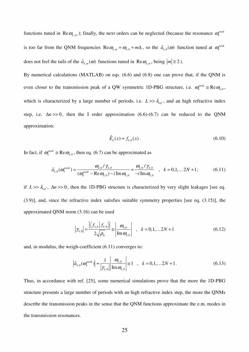
By numerical calculations (MATLAB) on eqs. (6.6) and (6.8) one can prove that, if the QNM is

even closer to the transmission peak of a QW symmetric 1D-PBG structure, i.e. ,0Repeak

k kω ω≅ ,

which is characterized by a large number of periods, i.e. ref

L λ>> , and an high refractive index

step, i.e. 0n∆ >> , then the I order approximation (6.6)-(6.7) can be reduced to the QNM

approximation:

,0( ) ( )k kE x f x≈ɶ . (6.10)

In fact, if ,0Repeak

k kω ω≅ , then eq. (6.7) can be approximated as

,0 ,0 ,0 ,0

,0

,0 ,0 ,0

/ /( ) , 0,1, 2 1

( Re ) Im Im

k k k kpeak

k k peak

k k k k

a k Ni i

ω γ ω γω

ω ω ω ω= ≈ = +

− − −ɶ … ; (6.11)

if ref

L λ>> , 0n∆ >> , then the 1D-PBG structure is characterized by very slight leakages [see eq.

(3.9)], and, since the refractive index satisfies suitable symmetry properties [see eq. (3.15)], the

approximated QNM norm (3.16) can be used

,0 ,0 ,0

,0

,00

, 0,1, 2 1Im2

k k k

k

k

f fk N

ωγ

ωρ= ≅ = +… (6.12)

and, in modulus, the weigh-coefficient (6.11) converges to:

,0

,0

,0,0

1( ) 1 , 0,1, 2 1

Im

kpeak

k k

kk

a k Nω

ωωγ

≈ ≅ = +ɶ … . (6.13)

Thus, in accordance with ref. [25], some numerical simulations prove that the more the 1D-PBG

structure presents a large number of periods with an high refractive index step, the more the QNMs

describe the transmission peaks in the sense that the QNM functions approximate the e.m. modes in

the transmission resonances.

26

In fig. 4, with reference to a QW symmetric 1D-PBG structure ( 1ref

mλ µ= , 6N = , 3h

n = , 2l

n = ),

the e.m. “mode” intensities (a) I band edgeI − at the low frequency band edge ( / 0.822

I band edge refω ω− = )

and (b) II band edgeI − at the high frequency band edge ( / 1.178

II band edge refω ω− = ), in units of the

intensity for an incoming pump pump

I , are plotted as functions of the dimensionless space /x L ,

where L is the length of the 1D-PBG structure. It is clear the shifting between the QNM

approximation (6.10) (the e.m. mode intensity I band edgeI − is due to QNM close to the band-edge) and

the first order approximation (6.6)-(6.7) [more refined than (6.10), band edge

I − is calculated as the

product of the QNM, close to the frequency band-edge, for a weigh coefficient, which takes into

account the shift between the band-edge resonance and the QNM frequency] or the second order

approximation (6.8)-(6.9) [even more refined, but almost superimposed to (6.6)-(6.7), band edge

I − is

calculated as the sum of the first order contribution due to the QNM, close to the frequency band-

edge, and the second order contributions of the two adjacent QNMs, with the same imaginary part,

so belonging to the same QNM family].

7. Quarter wave (QW) symmetric 1D-PBG structures

excited by two counter-propagating field pumps.

Let us consider a QW symmetric 1D-PBG structure with N periods and ref

ω as reference

frequency. If the universe includes the terminal surfaces of the 1D-PBG, the cavity is represented

as [0, ]C L= and the rest of universe as ( ,0) ( , )U L= −∞ ∪ ∞ . The 1D-PBG presents a refractive

index ( )n x which satisfies the symmetry properties ( / 2 ) ( / 2 )n L x n L x− = + . The cavity is

characterized by a transmission spectrum with 2 1N + resonances in the [0,2 )ref

ω range [23,24],

i.e. ( ) exp[ ], ( ) 0, 0,1, 2k k k k

t i r k Nω ω ϕ ω∃ ⇒ = = = …� [34].

27

Let us consider one pump, coming from the left side, which is tuned at the thk resonance of

the 1D-PBG structure, with unit amplitude and zero initial phase

( )

0( ) exp( )kk

p x in xc

ω→ =ɶ , (7.1)

being 0n the refractive index of the universe. It excites in the cavity an e.m. “mode” ( ) ( )k

E x→ɶ which

satisfies the equation [27]

22 ( )2 ( )

2( ) ( ) 0k k

k

d En x E x

dx c

ω→→ + =

ɶɶ , (7.2)

and the boundary conditions are [27]:

( ) ( ) ( ) ( ) ( )

( ) ( )

(0) (0) ( ) (0) (0) 1

( ) ( ) (0) ( )

k k k k k

k k k k

E p r p p

E L t p t

ω

ω ω

→ → → → →

→ →

= + = =

= =

ɶ ɶ ɶ ɶ

ɶ ɶ. (7.3)

Let us consider another pump, coming from the right side, tuned at the thk resonance of the

1D-PBG structure with unit amplitude and constant phase-difference ϕ∆ , i.e.

( )

0( ) exp[ ( )( )]exp[ ]k k

p x in c x L iω ϕ← = − − − ∆ɶ . (7.4)

If alone, this pump excites in the cavity an e.m. “mode” ( ) ( )k

E x←ɶ which satisfies an equation similar

to (7.2) [27]

22 ( )2 ( )

2( ) ( ) 0k k

k

d En x E x

dx c

ω←← + =

ɶɶ , (7.5)

because of the symmetry properties of the refractive index, with boundary conditions which are

different from (7.3) [27]:

( ) ( ) ( ) ( ) ( )

( ) ( )

( ) ( ) ( ) ( ) ( ) exp[ ]

(0) ( ) ( ) ( )exp[ ]

k k k k k

k k k k

E L p L r p L p L i

E t p L t i

ω ϕ

ω ω ϕ

← ← ← ← ←

← ←

= + = = − ∆

= = − ∆

ɶ ɶ ɶ ɶ

ɶ ɶ. (7.6)

It is easy to verify that the e.m. mode ( ) ( )k

E x←ɶ , which is excited by the pump (7.4) and solves the

equation (7.5) with the boundary conditions (7.6), is related to the e.m. mode ( ) ( )k

E x→ɶ , which is

excited by the pump (7.1) and solves equation (7.2) with the boundary conditions (7.3), by the link:

28

( ) ( )( ) [ ( )] ( ) exp[ ]k k k

E x E x t iω ϕ← → ∗= − ∆ɶ ɶ . (7.7)

The two counter-propagating pumps, which are tuned at the thk resonance of the 1D-PBG

structure, excite an e.m. “mode” ( )k

E xɶ inside the cavity, which is the linear super-position of

( ) ( )k

E x→ɶ and ( ) ( )

kE x

←ɶ , i.e. [27]

( ) ( ) ( ) ( )( ) ( ) ( ) ( ) [ ( )] ( ) exp[ ] k k k k k k

E x E x E x E x E x t iω ϕ→ ← → → ∗= + = + − ∆ɶ ɶ ɶ ɶ ɶ . (7.8)

It is easy to calculate from (7.8) the e.m. mode intensity inside the cavity [27]

( ) 2

( ) ( )

( ) 2 ( )

( ) ( )[ ( )]

2 ( ) 2 Re{[ ( )] ( ) exp[ ]}

2 ( ){1 cos[2 ( ) ]}

4 ( )cos [ ( ) ]2

k k k

k k k

k k k

kk k

I x E x E x

I x E x t i

I x x

I x x

ω ϕ

φ ϕ ϕϕ ϕφ

∗

→ ∗

→ →

→ →

= =

= + ∆ =

= + + ∆ − =∆ −

= +

ɶ ɶ ɶ

ɶ ɶ

ɶ

ɶ

, (7.9)

if the e.m. mode excited by the pump (7.1) is represented by ( ) ( ) ( )( ) ( ) exp[ ( )]k k kE x I x i xφ→ → →=ɶ ɶ .

Eq. (7.9) shows that the e.m. field generated by two monochromatic counter-propagating pump

waves leads to interference effects inside a QW symmetric 1D-PBG structure.

7.1. Density of modes (DOM).

In fig. 5, with reference to a symmetric QW 1D-PBG structure ( 1ref

mλ µ= , 6N = , 3h

n = ,

2l

n = ), the “e.m. mode” intensity excited inside the open cavity by one field pump (- - -) coming

from the left side [I order approximation (6.6)] and by two counter-propagating field pumps in

phase (—) [see eq. (7.9)] are compared when each of the two field pumps are tuned at (a) the low

frequency band-edge ( / 0.822I band edge ref

ω ω− = ) or (b) the high frequency band-edge

( / 1.178II band edge ref

ω ω− = ). The e.m. mode intensities I band edgeI − and II band edge

I − , in units of the

intensity for the two pumps pump

I , are plotted as functions of the dimensionless space /x L , where

L is the length of the 1D-PBG structure. If the two counter-propagating field pumps in phase are

29

tuned at the low frequency band-edge, there is a constructive interference and the field distribution

in that band-edge is reminiscent of the distribution excited by one field pump in the same

transmission peak; while, if the two pumps are tuned at the high frequency band-edge, there is a

destructive interference and almost no e.m. field penetration occurs in the structure.

Some numerical simulations on eq. (7.9) prove that, when a QW symmetric 1D-PBG structure with

N periods is excited by two counter-propagating field pumps with a phase-difference ϕ∆ , if N is

an even number, the e.m. mode intensities in the low (high) frequency band-edge increases in

strength when the two field pumps are in phase 0ϕ∆ = (out of phase ϕ π∆ = ) and almost flags

when the two pumps are out phase ϕ π∆ = (in phase 0ϕ∆ = ). Moreover, if N is an odd number,

the two field distributions in the low and high frequency band-edges exchange their physical

response with respect to the phase-difference of the two pumps. The duality between the field

distributions in the two band-edges, for which the one increases in strength when the other almost

flags, can be explained recalling that the transmission phases of the two band edges are such that

their sum is π ( π− ) when N is an odd (even) number.

Therefore, if a 1D-PBG structure is excited by two counter-propagating field pumps which are

tuned at one transmission resonance, no e.m. “mode” can be produced because it depends not only

on the boundary conditions (the two field pumps) but also on the initial conditions (the phase-

difference of the two pumps) [26]. We conjecture that the “density of modes” is a dynamic variable

which has the flexibility of varying with respect to the boundary conditions as well as the initial

conditions, in accordance with ref. [26].

8. A final discussion.

The Quasi Normal Mode (QNM) theory considers the realistic situation in which an optical

cavity is open from both sides and is enclosed in an infinite homogeneous external space; the lack

30

of energy conservation for optical open cavities gives resonance field eigen-functions with complex

eigen-frequencies. The time-space evolution operator for the cavity is not hermitian: the modes of

the field are quasi-normal, i.e. they form an orthogonal basis only inside the cavity.

The behavior of the electromagnetic field in the optical domain, inside one-dimensional photonic

crystals, is analyzed by using an extension of the QNM theory. One-dimensional (1D) Photonic

Band Gap (PBG) structures are particular optical cavities, with both sides open to the external

environment, with a stratified material inside. These 1D-PBG structures are finite in space and,

when we work with electromagnetic pulses of a spatial extension longer than the length of the

cavity, the 1D-PBG cannot be studied as an infinite structure: rather we have to consider the

boundary conditions at the two ends of the cavity.

In the present paper, the QNM approach has been applied to a double-side opened optical

cavity, and specified for a 1D-PBG structure. All the considerations made are exhaustively

demonstrated and all the subsequently results agree with the ones presented in literature [23-25].

In this paper (sec. 2), suitable “outgoing wave” conditions for an open cavity without external

pumping are formalized [see eqs. (2.2)-(2.3)]. More explicitly than refs. [8-15], here we have

considered a Laplace transform of the e.m. field, to take the cavity leakages into account, and we

have remarked that, only in the complex domain defined by a 2π -rotated Laplace transform, the

QNMs can be defined as the poles of the transformed Green function, with negative imaginary part.

Our iter has followed three steps:

1. the 2π -rotated Laplace transform of the e. m. field [see eqs. (2.4)-(2.5)] converges to an

analytical function ( , )E x ωɶ only over the half-plane of convergence Im 0ω > .

2. just because of the “asymptotic conditions” [see eq. (2.12)], the “auxiliary functions”

( , )g x ω± [see eq. (2.11)] are linearly independent over the half-plane of convergence

Im 0ω > , and so the Laplace transformed Green function ( , , )G x x ω′ɶ [see eq. (2.9)] is

analytic over Im 0ω > .

31

3. Differently from refs. [8-15], here we have remarked that: the transformed Green function

( , , )G x x ω′ɶ [see eq. (2.14)] can be extended also over the lower complex half-plane

Im 0ω < , for analytical continuation [28]; and, it is always possible to define an infinite set

of frequencies which are the poles of the transformed Green function ( , , )G x x ω′ɶ [see eqs.

(2.15)-(2.16)], over the lower complex half-plane Im 0ω < , according to ref. [30].

Moreover (sec. 3), if the open cavity is characterized by very slight leakages and its refractive index

satisfies suitable symmetry properties, more than refs. [8-15], here we have proved that the modulus

of the QNM norm in modulus can be expressed only in terms of the QNM frequencies [see eq.

(3.16)] and, more than refs. [23-25], here we have proposed its physical interpretation: the QNM

norm is high when the leakages of the open cavity are very slight; the QNM theory can be applied

to open cavities and is based on the “outgoing waves” conditions which formalize some leakages

( Im 0n

ω < ), so the QNM theory can not include the conservative case, when the cavities are closed

and are not characterized by any leakages ( Im 0n

ω = ).

The paper (sec. 4) has given a proof that the transmission coefficient ( )t ω can be calculated as a

superposition of suitable functions, with QNM norms n nf f as weighting coefficients and QNM

frequencies n

ω as parameters [see eq.(4.10)], thesis only postulated in ref. [25].

The QNM approach has been applied to a 1D-PBG structure (sec. 5): more than ref. [25], here the

transmission coefficient of a quarter wave (QW) symmetric 1D-PBG structure, with N periods and

refω as reference frequency, has been calculated as a superposition of 2 1N + QNM-cosecants,

which correspond to the number of QNMs in [0,2 )ref

ω range [see eq. (5.7)]; differently from the

assertion of ref. [21] for which the frequency dependence of ( )t ω could suggest at first glance that

the positions of maxima of 2

( ) ( )T tω ω= are realized when the real frequency coincides with the

real part of the QNM frequencies n

ω , here we have deduced that this fact is true only in the further

hypothesis of real parts of QNM frequencies n

ω well separated on the real frequency axis, whereas,

32

on the contrary, overlapping of the tails of two near QNM-cosecant contributions to ( )T ω lead to a

significantly displayed position of the maxima of ( )T ω , a sort of aliasing process (see figs. 4.a-c.

and tab. 1.a-c.).

In sec. 6., the transmission resonances have been compared with the QNM frequencies (sec. 6.a.)

and the transmission “modes” in the resonances have been calculated as super-positions of the

QNM functions (sec. 6.b.): differently from ref. [22], here we affirm explicitly that a proper field

representation for the transmittance problem can be established in terms of QNMs, and the

boundary conditions are not violated [see eqs. (6.2)-(6.3)]; even if the fields are entirely different

when considered on the whole real axis, the e.m. field can be represented as a superposition of

QNMs inside the open cavity and on the limiting surfaces too.

In the present paper (sec. 7), it has been shown that the e.m. field generated by two

monochromatic counter-propagating pump waves leads to interference effects inside a QW

symmetric 1D-PBG structure [see eq. (7.9)].

Even if this paper is chronologically subsequent to ref. [25], anyway it is conceived as a trait

d’union between refs. [25] and [26], in fact the paper forestalls conceptually, according to classic

electrodynamics, what ref. [26] develops in terms of quantum mechanics.

We have shown that if a 1D-PBG structure is excited by two counter-propagating pumps which are

tuned at one transmission resonance, no e.m. mode can be produced because it depends not only on

the boundary conditions (the two pumps) but also on the initial conditions (the phase-difference of

the two pumps) [see fig. 5.a-b.]; in accordance with ref. [26], we have conjectured (sec 7.1) that the

density of the modes (DOM) is a dynamical variable which has the flexibility to adjust with respect

to the boundary conditions as well the initial conditions.

In Appendix, a direct method has been described to obtain the QNM norm for a QW

symmetric 1D-PBG structure: the QNM norm n nf f can be obtained in terms of the n

ω

33

frequency and of the 2 2 ( )N

A ω+ , 2 2 ( )N

B ω+ coefficients for the ( , )g x ω− auxiliary function in the

2 2NL + layer on the right side of the 1D-PBG structure.

8.1. A comparison with Maksimovic et al. ref. [22].

Let us propose a critical comparison between Maksimovic and our methods:

• Maksimovic specializes ref. [22] to finite periodic structures which possess transmission

properties with a bandgap, i.e. with a region of frequencies of very low transmission. Ref.

[22] chooses a field model for the transmittance problem and takes the relevant QNMs as

those with the real part of their complex frequency in the given frequency range. To

determine the decomposition coefficients in the field model, a variational form of the

transmittance problem is employed. The transmittance problem corresponds to the equation

and natural boundary conditions, arising form the condition of stationarity of a functional

[ ( , )]F E x t . If [ ( , )]F E x t becomes stationary, i.e. if the first variation of [ ( , )]F E x t vanishes

for arbitrary variations of the e.m. field ( , )E x t , then ( , )E x t satisfies the natural boundary

conditions. The optimal coefficients can be obtained as solutions of a system of linear

equations. By solving the system for each value of the real frequency, the decomposition

coefficients in the field representation for transmittance problem are obtained. This enables

approximation of the spectral transmittance and reflectance and the related field profile.

Maksimovic applies a method which is based on a mathematical principle, involving

arduous calculations. Instead, we have proposed, for an open cavity, a physical method

which starts from the boundary conditions at the surfaces of the cavity (sec. 4). Moreover,

we have provided, for a symmetric 1D-PBG structure (sec. 5), a new algorithm to calculate

the QNM norm by a derivative [see eq. (5.2)], more direct than the integral of ref. [22]; and,

we have proved that a QW symmetric 1D-PBG structure with N periods is characterized by

34

2 1N + families of QNM frequencies, periodically distributed on the complex plane, such

that, for each family, the QNM norm is periodical with a proper step [see eq. (5.4)]: as a

result, the calculation of the transmission coefficient is even more simplified with respect to

ref. [22].

• A common assumption made in the literature [8-15][20][23,24][35] is that the spectral

transmission for single resonance situation, as described, is of a Lorentian like shape. We

have fallen into line of this assumption (sec. 6.b): in fact, the e.m. field, inside a QW

symmetric 1D-PBG structure, has been calculated as a superposition of QNMs; so, each

single resonance is described by a Lorentian like shape [see eqs. (6.3), (6.4)-(6.5) and

comments below].

The method of ref. [22] justifies analytically this common assumption. Maksimovic

considers the contribution of a single QNM in the field model. Here (sec. 6.b.), we have

considered the contributions of the adjacent QNMs, by more and more refined

approximations including successive orders: in fact, some numerical simulations have

proved that (see figs. 4.a-b.), when the transmission peak is close to the QNM, it is sufficient

to calculate the transmission mode by the I order approximation [see eqs. (6.6)-(6.7)],

otherwise, by the II order approximation, more refined [see eqs. (6.8)-(6.9) and comments

below]; so, in our opinion, the contribution of a single QNM is sufficient for the field model

only in the limit of narrow resonances [see eqs. (6.10), (6.11)-(6.13) and comments below] .

Appendix: QNM norm for 1D-PBG structures.

With reference to fig.2, let us now consider a symmetric one dimensional photonic band gap

(1D-PBG) structure which consists of N period plus one layer; every period is composed of two

35

layers respectively with lengths h and l and with refractive indices h

n and l

n , while the added layer

is with parameters h and h

n .

The symmetric 1D-PBG structure consists of 2 1N + layers with a total length ( )L N h l h= + + . If

the two layers external to the symmetric 1D-PBG structure are considered, the 1D-space x can be

divided into 2 3N + layers; the two external layers, 0 ( ,0)L = −∞ and 2 2 ( , )N

L L+ = +∞ , and the 1D-

PBG layers, the odd ones 2 1 [( 1)( ), ( 1)( ) ], 1,2, , 1k

L k h l k h l h k N− = − + − + + = +… and the even

ones 2 [( 1)( ) , ( )], 1,2, ,k

L k h l h k h l k N= − + + + = … .

The refractive index ( )n x takes a constant value k

n in every layer , 0,1, , 2 1,2 2k

L k N N= + +… ,

i.e.

0 0 2 2 for ,

( ) for , 1,3, ,2 1,2 1

for , 2,4, ,2

N

h k

l k

n x L L

n x n x L k N N

n x L k N

+∈= ∈ = − + ∈ =

…

…

. (A.1)

At first, the calculation of quasi normal modes (QNMs) is stated for the 1D-PBG structure

with refractive index (A.1). The homogeneous equation is solved for the auxiliary functions (2.11),

with the "asymptotic conditions" (2.12). The auxiliary function ( , )g x ω− is

0 0

0

0 0

1

2 1 2 1

1

2 2

1

2 2

( , ) ( )

[ ( 1)( )] [( 1)( ) ]

[ ( 1)( ) ] [ ( ) ]

h h

l l

in x in xc c

Nin x in x

c ck k

k

N in x in xc c

k k

k

in xc

N

g x A e B e x

A e B e x k h l k h l h x

A e B e x k h l h k h l x

A e B

ω ω

ω ω

ω ω

ω

ω ϑ

ϑ ϑ

ϑ ϑ

−

−

+ −

− −=

−

=

+

= + − +

+ + − − + − + + − +

+ + − − + − + − +

+ +

∑

∑

0

2 2 ( )in x

cN

e x L

ω

ϑ−

+

−

, (A.2)

where ( )xϑ is the unit step function; while the auxiliary function ( , )g x ω+ has a similar expression

to (A.2), where some coefficients ( )k

C ω and ( )k

D ω replace ( )k

A ω and ( )k

B ω with

0,1, , 2 1,2 2k N N= + +… . The auxiliary function ( , )g x ω− is a “right to left wave” for 0x < , so

36

0 ( ) 0A ω = , while the auxiliary function ( , )g x ω+ is a “left to right wave” for x L> , so

2 2 ( ) 0N

D ω+ = .

If the continuity conditions are imposed at the 1D-PBG surfaces for the auxiliary function ( , )g x ω−

and its spatial derivative ( , )xg x ω−∂ , it follows

l l

h h

l l

h 01

0 0 01

h

in [(k 1)(h l) h ] in [(k 1)(h l) h]c c

in [(k 1)(h l) h ] inc

l2k

in [(k 1)(h l) h ] in [(k 1)(h l) h]2k c c

l

11

n 1 1 AA 1

n n BB 121

n

1e e

nA e e1

B 2 1e e

n

ω ω− − + + − − + +

ω− + + −

ω ω− + + − + +

= − −

= −

h h

h h

l l

h h

[(k 1)(h l) h]c

2k 1

in [(k 1)(h l) h ] in [(k 1)(h l) h ] 2k 1c ch h

in k(h l) in k(h l)c c

in k(h l) in k (hc c

h2k 1

in k(h l) in k(h l)2k 1 c c

h

A

Bn e n e

1e e

nA e e1

B 2 1e e

n

ω− + +

−

ω ω− + + − − + + −

ω ω− + − +

ω ω+ −

+

ω ω+ ++

−

= −

l l

0 0

h h

h h0 0

l)

2k

in k(h l) in k (h l) 2kc cl l

in L in Lc c

in L in Lc c

02N 2 2N 1

in L in Lin L in L2N 2 2N 1c cc ch h

0

A

Bn e n e

1e e

nA Ae e1

B B2 1n e n ee e

n

+

ω ω+ − +

ω ω− −

ω ω−

+ +

ω ωω ω−+ +

−

= −−

(A.3)

while the continuity conditions for ( , )g x ω+ are similar to (A.3), but the coefficients ( )k

C ω and

( )k

D ω replace ( )k

A ω and ( )k

B ω with 0,1, , 2 1,2 2k N N= + +… . The 0 ( )B ω coefficient is fixed

choosing a normalization condition and all the [ ( ), ( )]k k

A Bω ω couples with 1, , 2 2k N= +… are

determined applying the continuity conditions (A.3). Similarly for the 2 2 ( )N

C ω+ coefficient and

the [ ( ), ( )]k k

C Dω ω couples with 0,1, , 2 1k N= +… .

The QNM frequencies can be calculated, if suitable conditions are imposed to the ( , )g x ω±

coefficients. At QNM frequencies n

ω ω= , where Im 0n

ω < , the auxiliary functions ( , )g x ω± are

linearly dependent ( , ) ( , )g x g xω ω− +∝ ; they are “right to left waves” for 0x < , so 0 ( ) 0n

C ω = ,

and “left to right waves” for x L> , so:

37

2 2

2 2 2 2

( ) 0

( ) ( )

N n

N n N n

B

A C

ωω ω

+

+ +

= =

. (A.4)

Finally, the QNM norm can be calculated for the stratified medium with refractive index

(A.1). The Wronskian ( , )W x ω of the auxiliary functions ( , )g x ω± is obtained from eq. (2.13),

using eq. (A.2)

0 0 0 0

2 1 2 1 2 1 2 1 2 1

2 2 2 2 2

2 ( ) ( ) ,

2 [ ( ) ( ) ( ) ( )], , 1, , 1

( , )

2 [ ( ) ( ) ( ) ( )] , , 1, ,

h k k k k k

l k k k k k

in B C x Lc

in A D B C x L k Nc

W x

in A D B C x L k Nc

ω ω ω

ω ω ω ω ωω

ω ω ω ω ω

− − − − −

∈

− + ∈ = … +=

− + ∈ = …

0 2 2 2 2 2 22 ( ) ( ) , N N N

in B C x Lc

ω ω ω+ + +

∈

. (A.5)

The Wronskian ( , )W x ω is x-independent, for the equivalence of all the expressions (A.5), as it can

be proved using eq. (A.3), i.e.

0 2 2 2 2( ) 2 ( ) ( ), N N

W in B C xc

ωω ω ω+ += ∀ ∈ℝ . (A.6)

The QNM norm ( / )nn nf f dW d ω ωω == is obtained from eq. (A.6), using eq. (A.4), so:

2 20 2 22 ( )

n

n Nn n N n

dBf f in A

c d ω ω

ω ωω

++

=

=

. (A.7)

Acknowledgements

A. Settimi is particularly indebted to C. Sibilia and M. Bertolotti who proposed him the strand of

research about Quasi Normal Modes. Furthermore, the authors are sincerely grateful to A. Napoli

and A. Messina for the interesting discussions on QNMs .

38

References.

1. K. Sakoda, Optical Properties of Photonic Crystals (Springer Verlag, 2001).

2. J. Maddox, “Photonic band-gaps bite the dust”, Nature 348, 481-481 (1990).

3. S. John, “Strong localization of photons in certain disordered dielectric superlattices”, Phys. Rev.

Lett. 58, 2486-2489 (1987).

4. S. John, “Electromagnetic Absorption in a Disordered Medium near a Photon Mobility Edge”,

Phys. Rev. Lett. 53, 2169-2172 (1984).

5. P. Yeh, Optical Waves in Layered Media (Wiley, 1988).

6. M. Centini, C. Sibilia, M. Scalora, G. D’Aguanno, M. Bertolotti, M. J. Bloemer, C. M. Bowden,

and I. Nefedov, “Dispersive properties of finite, one-dimensional photonic band gap structures:

Applications to nonlinear quadratic interactions”, Phys. Rev. E 60, 4891-4898 (1999).

7. J. E. Sipe, L. Poladian, and C. Martijn de Sterke, “Propagation through nonuniform grating

structures”, J. Opt. Soc. Am. A 4, 1307-1320 (1994).

8. E. S. C. Ching, P. T. Leung, and K. Young, “Optical processes in microcavities - The role of

Quasi-Normal Modes”, in Optical processes in mirocavities, R. K. Chang and A. J. Campillo, eds.

(World Scientific, 1996), pp. 1-75.

9. P. T. Leung, S. Y. Liu, and K. Young, “Completeness and orthogonality of quasinormal modes in

leaky optical cavities”, Phys. Rev. A 49, 3057-3067 (1994).

10. P. T. Leung, S. S. Tong, and K. Young, “Two-component eigenfunction expansion for open

systems described by the wave equation I: completeness of expansion”, J. Phys. A: Math. Gen. 30,

2139-2151 (1997).

11. P. T. Leung, S. S. Tong, and K. Young, “Two-component eigenfunction expansion for open

systems described by the wave equation II: linear space structure”, J. Phys. A: Math. Gen. 30, 2153-

2162 (1997).

39

12. E. S. C. Ching, P. T. Leung, A. Maassen van den Brink, W. M. Suen, S. S. Tong, and K. Young,

“Quasinormal-mode expansion for waves in open systems”, Rev. Mod. Phys. 70, 1545-1554

(1998).

13. P. T. Leung, W. M. Suen, C. P. Sun, and K. Young, “Waves in open systems via a biorthogonal

basis”, Phys. Rev. E 57, 6101-6104 (1998).

14. K. C. Ho, P. T. Leung, Alec Maassen van den Brink, and K. Young, “Second quantization of

open systems using quasinormal modes”, Phys. Rev. E 58, 2965-2978 (1998).

15. Alec Maassen van den Brink and K. Young, “Jordan blocks and generalized bi-orthogonal

bases: realizations in open wave systems”, J. Phys. A: Math. Gen. 34, 2607-2624 (2001).

16. B. J. Hoenders, “On the Decomposition of the Electromagnetic Field into its Natural Modes”,

in Proceedings of the 4th Int. Conf. on Coherence and Quantum Optics, L.Mandel and E.Wolf, eds.

(Plenum Press, 1978), pp. 221-233 .

17. B. J. Hoenders and H. A. Ferwerda, “On a New proposal Concerning the Calculation of the

Derivatives of a Function Subject to Errors”, Optik 40, 14-17 (1974).

18. B. J. Hoenders, “Completeness of a set of modes connected with the electromagnetic field of a

homogeneous sphere embedded in an infinite medium”, J. Mat. Phys. 11, 1815-1832 (1978).

19. B. J. Hoenders, “On the completeness of the natural modes for quantum mechanical potential

scattering”, J. Mat. Phys. 20, 329-335 (1979).

20. M. Bertolotti, “Linear one-dimensional resonant cavities”, in Microresonators as building

blocks for VLSI photonics of AIP Conference Proceedings, F. Michelotti, A. Driessen, and M.

Bertolotti, eds. (AIP, 2004), Vol. 709, pp. 19-47.

21. B. J. Hoenders and M. Bertolotti, “The (quasi)normal natural mode description of the scattering

process by dispersive photonic crystals”, Proc. SPIE Int. Soc. Opt. Eng. 6182, 61821F-6182G

(2006).

40

22. M. Maksimovic, M. Hammer, and E. van Groesen, “Field representation for optical defect

resonances in multilayer microcavities using quasi-normal modes”, Optics Comm. 281, 1401-1411

(2008).

23. S. Severini, A. Settimi, N. Mattiucci, C. Sibilia, M. Centini, G. D'Aguanno, M. Bertolotti, M.

Scalora, M. J. Bloemer, and C. M. Bowden, “Quasi Normal Modes description of waves in 1D

Photonic Crystals”, in Photonics, Devices, and Systems II of SPIE Proceedings, M. Hrabovsky, D.

Senderakova and P. Tomanek, eds. (SPIE, 2003), Vol. 5036, pp. 392-401.

24. A. Settimi, S. Severini, N. Mattiucci, C. Sibilia, M. Centini, G. D’Aguanno, M. Bertolotti, M.

Scalora, M. Bloemer, C. M. Bowden, “Quasinormal-mode description of waves in one-dimensional

photonic crystals”, Phys. Rev. E 68, 026614 1-11 (2003).

25. S. Severini, A. Settimi, C. Sibilia, M. Bertolotti, A. Napoli, A. Messina, £Quasi-Normal

Frequencies in Open Cavities: An Application to Photonic Crystals”, Acta Phys. Hung. B 23/3-4,

135-142 (2005).

26. S. Severini, A. Settimi, C. Sibilia, M. Bertolotti, A. Napoli, A. Messina, “Quantum counter-

propagation in open optical cavities via the quasi-normal-mode approach”, Laser Physics, 16, 911-

920 (2006).

27. M. Born and E. Wolf, Principles of Optics (Macmillan, 1964).

28. G. F. Carrier, M. Krook, and C. E. Pearson, Functions of a complex variable – theory and

technique (McGraw-Hill Book Company, 1983).

29. E. N. Economou, Green’s functions in Quantum Physics (Springer-Verlag, 1979).

30. A. Bachelot, A. Motet-Bachelot, “Les résonances d'un trou noir de Schwarzschild”, Ann. Inst.

Henry Poincare 59, 3-68 (1993).

31. D. W. L. Sprung, H. Wu, and J. Martorell, “Scattering by a finite periodic potential”, Am. J.

Phys. 61, 1118-1124 (1993).

32. M. G. Rozman, P. Reineken, and R. Tehver, “Scattering by locally periodic one-dimensional

potentials”, Phys. Lett. A 187, 127-131 (1994).

41

33. J. M. Bendickson, J. P. Dowling, and M. Scalora, “Analytic expressions for the electromagnetic

mode density in finite, one-dimensional, photonic band-gap structures”, Phys. Rev. E 53, 4107-

4121 (1996).

34. J. P. Dowling, “Parity, time-reversal and group delay for inhomogeneous dielectric slabs:

Application to pulse propagation in finite, one-dimensional, photonic bandgap structures”, in

Proceedings of IEEE-Optoelctronics (IEEE ,1998), Vol. 145, pp. 420-435.

35. A. Sopahaluwakan, Characterization and simulation of localized states in periodic structures ,

Ph. D. Thesis (University of Twente, 2006).

42

Figures and captions

Figure 1.a.

Figure 1.b.

Open cavity

E(x,t)

x

n(x)

0 L

1

EP(x,t)

ER(x,t)

ET(x,t)

Open cavity

x

n(x)

0 L

1

ELeft(x,t) ERight(x,t)

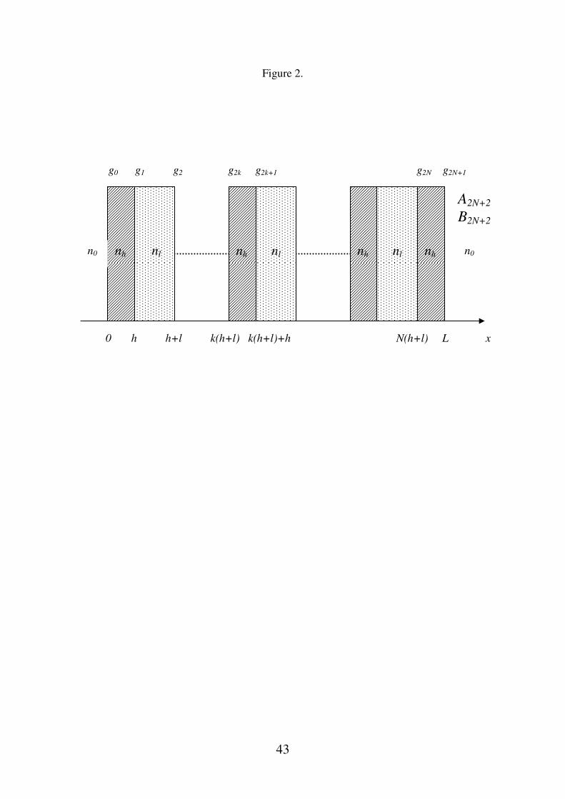
43

Figure 2.

0 h h+l k(h+l) k(h+l)+h N(h+l) L x

g0 g1 g2 g2k g2k+1 g2N g2N+1

nh

nl

nh

nl

nh

nl

nh n0 n0

A2N+2

B2N+2

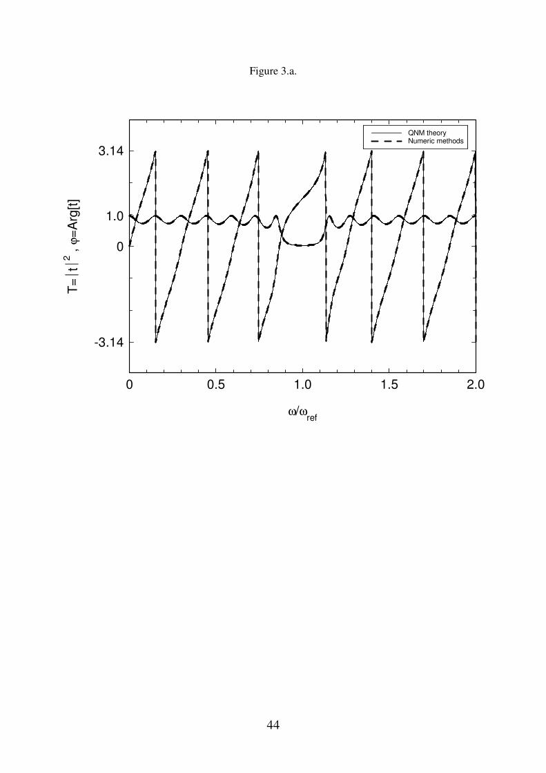
44

Figure 3.a.

-3.14

0

3.14

1.0

0 0.5 1.0 1.5 2.0

QNM theoryNumeric methods

ω/ωref

T=

t2

, ϕ

=A

rg[t

]

45

Figure 3.b.

-3.14

0

3.14

1.0

0 0.5 1.0 1.5 2.0

QNM theoryNumeric methods

ω/ωref

T=

t2

, ϕ

=A

rg[t

]

46

Figure 3.c.

-3.14

0

3.14

1.0

0 0.5 1.0 1.5 2.0

QNM theoryNumeric methods

ω/ωref

T=

t2

, ϕ

=A

rg[t

]

47

Table 1.a.

λref=1µm, N=6, nh=2, nl=1.5 Re(ωQNM/ωref) ωBand-Edge/ωref (ReωQNM-ωB.E.)/ωB.E. ∠t(ωB.E./ωref)

Low frequency

band-edge

0.834 0.846 -0.014 -0.8011

High frequency

band-edge

1.166 1.154 0.010 -2.341

Table 1.b.

λref=1µm, N=6, nh=3, nl=2 Re(ωQNM/ωref) ωBand-Edge/ωref (ReωQNM-ωB.E.)/ωB.E. ∠t(ωB.E./ωref)

Low frequency

band-edge

0.825 0.822 0.003 -0.6342

High frequency

band-edge

1.175 1.178 -0.002 -2.507

Table 1.c.

λref=1µm,N=7,nh=3,nl=2 Re(ωQNM/ωref) ωBand-Edge/ωref (ReωQNM-ωB.E.)/ωB.E. ∠t(ωB.E./ωref)

Low frequency

band-edge

0.853 0.832 0.025 2.528

High frequency

band-edge

1.147 1.168 -0.015 0.6135

48

Figure 4.a.

0

1

2

3

4

5

0 0.2 0.4 0.6 0.8 1.0

QNM approximationI order approximationII order approximation

x/L

I I band-e

dge/I

pum

p

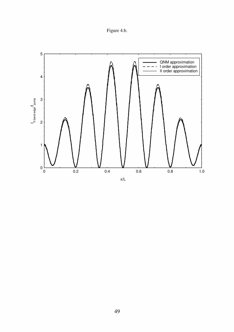
49

Figure 4.b.

0

1

2

3

4

5

0 0.2 0.4 0.6 0.8 1.0

QNM approximationI order approximationII order approximation

x/L

I II b

and-e

dge/I

pum

p

50

Figure 5.a.

0

5

10

15

0 0.2 0.4 0.6 0.8 1.0

one pumptwo pumps (∆ϕ=0)

x/L

I I band-e

dge/I

pum

p

51

Figure 5.b.

0

1

2

3

4

5

0 0.2 0.4 0.6 0.8 1.0

one pumptwo pumps (∆ϕ=0)

x/L

I II b

and-e

dge/I

pum

p

52

Figure 1. A cavity opened at both ends, of length L , with a refractive index ( )n x : (a) in absence of

external pumping, so electromagnetic field satisfies the “outgoing waves” conditions (2.2); (b) in

presence of a left-pump ),( txEP which satisfies the “incoming wave condition” (4.3).

Figure 2. Refractive index ( )n x for a symmetric 1D-PBG structure with N periods plus one layer;

every period is composed of two layers, respectively with lengths h and l and with refractive

indices h

n and l

n , while the added layer is with parameters h and h

n .

Figure 3. Transmission spectrum (squared modulus and phase) predicted by QNM theory (—) and

by numeric methods existing in the literature [31-33] (- - -) , for QW symmetric 1D-PBG

structures, with reference wavelength 1ref

mλ = µ and: (a) number of periods 6N = , refractive

indices 2, 1.5h l

n n= = ; (b) 6N = , refractive indices 3, 2h l

n n= = ; (c) 7N = , 3, 2h l

n n= = .

Table 1. Three examples of QW symmetric 1D-PBG structures are considered: (a) 1ref

mλ µ= ,

6N = , 2h

n = , 1,5l

n = , (b) 1ref

mλ µ= , 6N = , 3h

n = , 2l

n = , (c) 1ref

mλ µ= , 7N = , 3h

n = ,

2l

n = . For each of the three examples, the low and high frequency band-edges are described in

terms of their resonances ( /Band Edge ref

ω ω− ) and phases . .( / )B E ref

t ω ω∠ ; besides, there is one QNM

close to every single band-edge: the real part of the QNM-frequency Re( / )QNM ref

ω ω is reported

together with the relative shift from the band-edge resonance . . . .(Re ) /QNM B E B E

ω ω ω− .

Figure 4. With reference to a QW symmetric 1D-PBG structure ( 1ref

mλ µ= , 6N = , 3h

n = ,

2l

n = ), the e.m. “mode” intensities (a) I band edgeI − at the low frequency band edge

( / 0.822I band edge ref

ω ω− = ) and (b) II band edgeI − at the high frequency band edge

53

( / 1.178II band edge ref

ω ω− = ), in units of the intensity for an incoming pump pump

I , are plotted as

functions of the dimensionless space /x L , where L is the length of the 1D-PBG structure. It is clear

the shifting between the QNM approximation (6.10) (the e.m. mode intensity I band edgeI − is due to

QNM close to the band-edge) and the first order approximation (6.6)-(6.7) [more refined than (6.10)

, band edge

I − is calculated as the product of the QNM, close to the frequency band-edge, for a weigh

coefficient, which takes into account the shift between the band-edge resonance and the QNM

frequency] or the second order approximation (6.8)-(6.9) [even more refined, but almost

superimposed to (6.6)-(6.7), band edge

I − is calculated as the sum of the first order contribution due to

the QNM, close to the frequency band-edge, and the second order contributions of the two adjacent

QNMs, with the same imaginary part, so belonging to the same QNM family].

Figure 5. With reference to a QW symmetric 1D-PBG structure ( 1ref

mλ µ= , 6N = , 3h

n = ,

2l

n = ), the e.m. “mode” intensities excited inside the open cavity by one pump (- - -) coming from

the left side [I order approximation (6.6)] and by two counter-propagating pumps in phase (—) [see

eq. (7.9)] are compared when each of the two pumps are tuned at (a) the low frequency band-edge

( / 0.822I band edge ref

ω ω− = ) or (b) the high frequency band-edge ( / 1.178II band edge ref

ω ω− = ). The e.m.

mode intensities I band edgeI − and II band edge

I − , in units of the intensity for the two pumps pump

I are

plotted as functions of the dimensionless space /x L , where L is the length of the 1D-PBG

structure. Thus, two counter-propagating pumps tuned at the same transmission resonance do not

necessarily excite the cavity mode which one might expect at that frequency if the same pumps

have an appropriate phase-difference.