1

Quasi One-Dimensional Unsteady Modeling of External

Compression Supersonic Inlets

George Kopasakis1, and Joseph W. Connolly

2

NASA Glenn Research Center, Cleveland, Ohio 44135

Jonathan Kratz3

Ohio State University, Columbus, Ohio 43210

The AeroServoElasticity task under the NASA Supersonics Project is developing dynamic models of the

propulsion system and the vehicle in order to conduct research for integrated vehicle dynamic

performance. As part of this effort, a nonlinear quasi 1-dimensional model of an axisymmetric external

compression supersonic inlet is being developed. The model utilizes compressible flow computational

fluid dynamics to model the internal inlet segment as well as the external inlet portion between the cowl

lip and normal shock, and compressible flow relations with flow propagation delay to model the oblique

shocks upstream of the normal shock. The external compression portion between the cowl-lip and the

normal shock is also modeled with leaking fluxes crossing the sonic boundary, with a moving CFD

domain at the normal shock boundary. This model has been verified in steady state against tunnel inlet

test data and it’s a first attempt towards developing a more comprehensive model for inlet dynamics.

Nomenclature A = area, m

2

a = local speed of sound, m/s

aI = distance between the cowl-lip and centerbody at the inlets entrance, m

aL = distance between the cowl-lip and centerbody at the shocks location, m

F = ratio of sonic mass flux to mass flux across the assumed sonic line, used for flux spillages

FC = adjustment to F for variable geometries

Fj = flux term

hT = total enthalpy, (J/kg)

J = 0 if 2D inlet, 1 if axially symmetric inlet

M = Mach number

ṁ = mass flow rate, (kg/s)

P = pressure, (N/m2)

R = universal gas constant, (N*m)/(kg*K)

RCB = radius or distance of the edge of the centerbody to the center of the centerbody, m

Rshk = radius or distance of the edge of the oblique shock fan to the center of the centerbody, m

R∞ = radius or distance of cell boundary level at the cowl-lip to the center of the centerbody, m

Sj = source term

Sv = coefficient for artificial viscosity term

v = velocity, m/s

T = temperature, K

YC = distance for the center of the centerbody to the cowl-lip height, m

Wj = states term

x = centerbody x-coordinate, m

y = centerbody y-coordinate, m

1 Senior Controls Engineer, Communications Instrumentation and Controls Division, 21000 Brookpark Rd/77-1, AIAA Member. 2 Aerospace Engineer, Communications Instrumentation and Controls Division , 21000 Brookpark Rd/77-1, AIAA Member. 3 Student, Aerospace Engineering Program

https://ntrs.nasa.gov/search.jsp?R=20120018047 2018-06-17T07:01:33+00:00Z

2

Greek a = blunt body half width, m

β = shock angle, deg.

Δ = change in variable

ρ = density, kg/m3

γ = ratio of specific heats

θ = local incidence angle to the free stream, deg.

δ = shock standoff distance, m

ξ = shock sensing factor

ν = Prantl-Meyer function operator

Subscripts B = bleed flow

e = exit of the inlet

j = corresponding conservation equation for CFD states, fluxes, and sources

i = current cell

n = cell number

S = secondary flow

s = static condition

sp = spilled over the cowl-lip

T = total condition

∞ = free-stream condition

I. Introduction

UPERSONIC external compression inlets are considered for lower supersonic cruise speeds (M=1.8 or below), due to their

overall performance associated with propulsion efficiency, weight, and complexity (no bypass actuators for shock control).

A supersonic external compression inlet compresses air through a series of oblique shocks followed by a normal shock where the

flow transitions from supersonic to subsonic. After the normal shock occurs somewhere outside the inlet or by the cow-lip, the

flow travels at subsonic speeds to the entrance of the inlet or inside the inlet. At the design point, the normal shock is at the cowl-

lip and for most off design operation the shock is somewhere upstream of the cowl-lip. Some of the flow between the normal

shock and the cowl-lip escapes overboard or is bypassed and the rest enters the enclosed portion of the inlet which is essentially

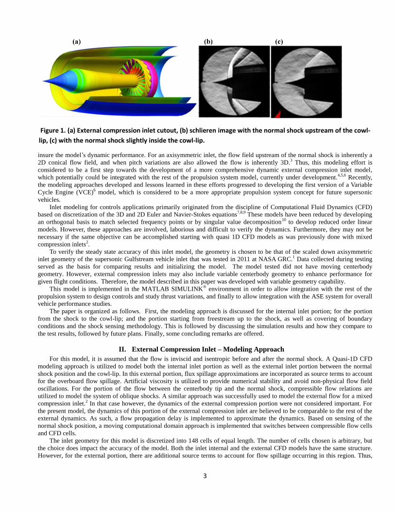
a subsonic diffuser, before the flow finally enters the engine. Figure 1 shows (a) a cutout of the external compression inlet with a

dual flow stream configuration, also showing the engine fan; (b) a test schlieren image with the normal shock positioned

upstream of the cow-lip, showing the flow spillage; and (c) a schlieren image with the normal shock positioned slightly inside

the cowl-lip. The flow upstream of the normal shock (to the left) is a conical flow, typical for axisymmetric type inlets. Testing

of this type of axisymmetric inlet was carried out at NASA Glenn Research Center (GRC), separately for a single and for a dual

flow path configuration. More detail on the testing that was done and the results can be found in Ref. [1]. The modeling and the

results in this paper are carried out only for the single flow path configuration.

Previously, a model was developed for mixed compression inlets2, which has some similarities to external compression

inlets and thus, the mixed compression inlet model serves as a starting point for this modeling effort. In the present effort, a quasi

1-Dimensional (1D) supersonic inlet model is developed for external compression inlets. This model utilizes compressible flow

Computational Fluid Dynamics (CFD) to solve the Euler governing equations for both the internal and external portions of the

flow at, and downstream of, the normal shock assuming isentropic flow conditions before and after the shock. For the oblique

shocks upstream of the normal shock, compressible flow relations are utilized with flow propagation delay for the dynamics. The

portion of the inlet geometry between the normal shock and the cowl lip also models the leakage flow as mass, momentum and

energy fluxes that escape across the sonic boundary. The CFD and the compressible flow boundaries are constructed as moving

domains to accommodate movement of the normal shock. The modeling approach utilizes central differencing to solve the

spatial CFD derivatives. It also assumes ideal gas with no friction or viscous effects. However, artificial viscosity is implemented

in this model to damp shock oscillations and to generate a numerically stable solution. This model also includes variable area

associated with variable centerbody geometry.

One of the purposes of developing this model is to include the gas dynamics necessary to develop improved control designs,

in order to more accurately design engine controls and also to capture the thrust dynamics of the propulsion system. The thrust

dynamics are needed to be able to integrate the propulsion system with the rest of the vehicle AeroServoElastic (ASE) modes in

order to study integrated vehicle performance for ride quality, stability, and efficiency. The model here is verified for steady state

performance against test data obtained from recent inlet testing conducted at NASA GRC. Ultimately, the objective is to also

S

3

insure the model’s dynamic performance. For an axisymmetric inlet, the flow field upstream of the normal shock is inherently a

2D conical flow field, and when pitch variations are also allowed the flow is inherently 3D.3 Thus, this modeling effort is

considered to be a first step towards the development of a more comprehensive dynamic external compression inlet model,

which potentially could be integrated with the rest of the propulsion system model, currently under development.4,5,6

Recently,

the modeling approaches developed and lessons learned in these efforts progressed to developing the first version of a Variable

Cycle Engine (VCE)6 model, which is considered to be a more appropriate propulsion system concept for future supersonic

vehicles.

Inlet modeling for controls applications primarily originated from the discipline of Computational Fluid Dynamics (CFD)

based on discretization of the 3D and 2D Euler and Navier-Stokes equations7,8,9

These models have been reduced by developing

an orthogonal basis to match selected frequency points or by singular value decomposition10

to develop reduced order linear

models. However, these approaches are involved, laborious and difficult to verify the dynamics. Furthermore, they may not be

necessary if the same objective can be accomplished starting with quasi 1D CFD models as was previously done with mixed

compression inlets2.

To verify the steady state accuracy of this inlet model, the geometry is chosen to be that of the scaled down axisymmetric

inlet geometry of the supersonic Gulfstream vehicle inlet that was tested in 2011 at NASA GRC.1 Data collected during testing

served as the basis for comparing results and initializing the model. The model tested did not have moving centerbody

geometry. However, external compression inlets may also include variable centerbody geometry to enhance performance for

given flight conditions. Therefore, the model described in this paper was developed with variable geometry capability.

This model is implemented in the MATLAB SIMULINK® environment in order to allow integration with the rest of the

propulsion system to design controls and study thrust variations, and finally to allow integration with the ASE system for overall

vehicle performance studies.

The paper is organized as follows. First, the modeling approach is discussed for the internal inlet portion; for the portion

from the shock to the cowl-lip; and the portion starting from freestream up to the shock, as well as covering of boundary

conditions and the shock sensing methodology. This is followed by discussing the simulation results and how they compare to

the test results, followed by future plans. Finally, some concluding remarks are offered.

II. External Compression Inlet – Modeling Approach

For this model, it is assumed that the flow is inviscid and isentropic before and after the normal shock. A Quasi-1D CFD

modeling approach is utilized to model both the internal inlet portion as well as the external inlet portion between the normal

shock position and the cowl-lip. In this external portion, flux spillage approximations are incorporated as source terms to account

for the overboard flow spillage. Artificial viscosity is utilized to provide numerical stability and avoid non-physical flow field

oscillations. For the portion of the flow between the centerbody tip and the normal shock, compressible flow relations are

utilized to model the system of oblique shocks. A similar approach was successfully used to model the external flow for a mixed

compression inlet.2 In that case however, the dynamics of the external compression portion were not considered important. For

the present model, the dynamics of this portion of the external compression inlet are believed to be comparable to the rest of the

external dynamics. As such, a flow propagation delay is implemented to approximate the dynamics. Based on sensing of the

normal shock position, a moving computational domain approach is implemented that switches between compressible flow cells

and CFD cells.

The inlet geometry for this model is discretized into 148 cells of equal length. The number of cells chosen is arbitrary, but

the choice does impact the accuracy of the model. Both the inlet internal and the external CFD models have the same structure.

However, for the external portion, there are additional source terms to account for flow spillage occurring in this region. Thus,

Figure 1. (a) External compression inlet cutout, (b) schlieren image with the normal shock upstream of the cowl-

lip, (c) with the normal shock slightly inside the cowl-lip.

4

the CFD portion of the model for the internal inlet (diffuser) portion will be covered first. This will be followed by the CFD

model for the external inlet portion. Finally, the model for the compressible flow region will be covered together with the

boundary conditions between these two flow regions. The discussion will also cover the logic used to determine how to switch

cells between compressible flow and CFD depending on the position of the normal shock.

A. Quasi-1D, Inviscid, Computational Fluid Dynamics for the Internal Inlet Portion

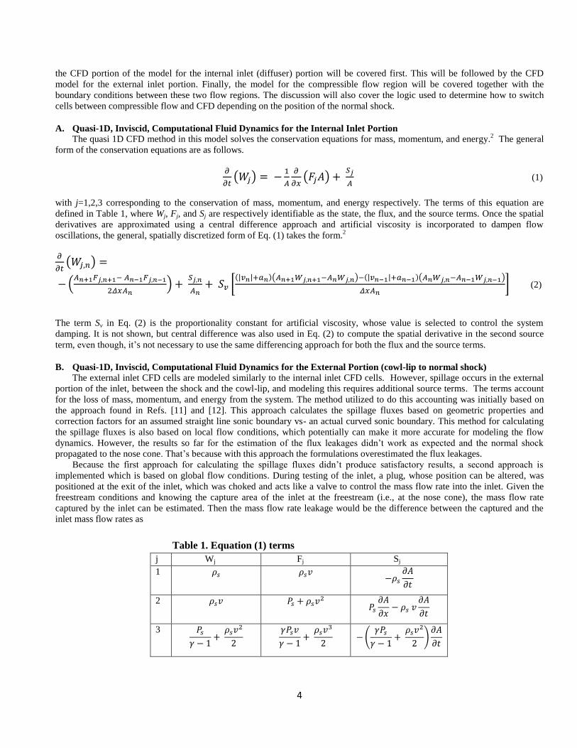
The quasi 1D CFD method in this model solves the conservation equations for mass, momentum, and energy.2 The general

form of the conservation equations are as follows.

(1)

with j=1,2,3 corresponding to the conservation of mass, momentum, and energy respectively. The terms of this equation are

defined in Table 1, where Wj, Fj, and Sj are respectively identifiable as the state, the flux, and the source terms. Once the spatial

derivatives are approximated using a central difference approach and artificial viscosity is incorporated to dampen flow

oscillations, the general, spatially discretized form of Eq. (1) takes the form.2

(2)

The term Sv in Eq. (2) is the proportionality constant for artificial viscosity, whose value is selected to control the system

damping. It is not shown, but central difference was also used in Eq. (2) to compute the spatial derivative in the second source

term, even though, it’s not necessary to use the same differencing approach for both the flux and the source terms.

B. Quasi-1D, Inviscid, Computational Fluid Dynamics for the External Portion (cowl-lip to normal shock)

The external inlet CFD cells are modeled similarly to the internal inlet CFD cells. However, spillage occurs in the external

portion of the inlet, between the shock and the cowl-lip, and modeling this requires additional source terms. The terms account

for the loss of mass, momentum, and energy from the system. The method utilized to do this accounting was initially based on

the approach found in Refs. [11] and [12]. This approach calculates the spillage fluxes based on geometric properties and

correction factors for an assumed straight line sonic boundary vs- an actual curved sonic boundary. This method for calculating

the spillage fluxes is also based on local flow conditions, which potentially can make it more accurate for modeling the flow

dynamics. However, the results so far for the estimation of the flux leakages didn’t work as expected and the normal shock

propagated to the nose cone. That’s because with this approach the formulations overestimated the flux leakages.

Because the first approach for calculating the spillage fluxes didn’t produce satisfactory results, a second approach is

implemented which is based on global flow conditions. During testing of the inlet, a plug, whose position can be altered, was

positioned at the exit of the inlet, which was choked and acts like a valve to control the mass flow rate into the inlet. Given the

freestream conditions and knowing the capture area of the inlet at the freestream (i.e., at the nose cone), the mass flow rate

captured by the inlet can be estimated. Then the mass flow rate leakage would be the difference between the captured and the

inlet mass flow rates as

Table 1. Equation (1) terms

j Wj Fj Sj

1

2

3

5

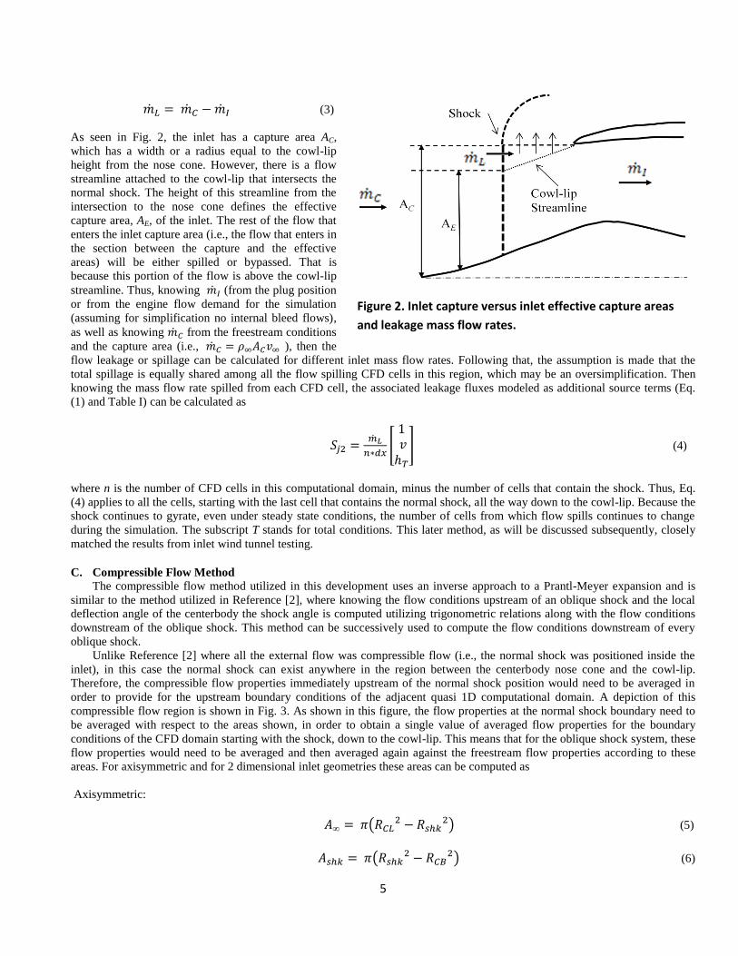
(3)

As seen in Fig. 2, the inlet has a capture area AC,

which has a width or a radius equal to the cowl-lip

height from the nose cone. However, there is a flow

streamline attached to the cowl-lip that intersects the

normal shock. The height of this streamline from the

intersection to the nose cone defines the effective

capture area, AE, of the inlet. The rest of the flow that

enters the inlet capture area (i.e., the flow that enters in

the section between the capture and the effective

areas) will be either spilled or bypassed. That is

because this portion of the flow is above the cowl-lip

streamline. Thus, knowing (from the plug position

or from the engine flow demand for the simulation

(assuming for simplification no internal bleed flows),

as well as knowing from the freestream conditions

and the capture area (i.e., ), then the

flow leakage or spillage can be calculated for different inlet mass flow rates. Following that, the assumption is made that the

total spillage is equally shared among all the flow spilling CFD cells in this region, which may be an oversimplification. Then

knowing the mass flow rate spilled from each CFD cell, the associated leakage fluxes modeled as additional source terms (Eq.

(1) and Table I) can be calculated as

(4)

where n is the number of CFD cells in this computational domain, minus the number of cells that contain the shock. Thus, Eq.

(4) applies to all the cells, starting with the last cell that contains the normal shock, all the way down to the cowl-lip. Because the

shock continues to gyrate, even under steady state conditions, the number of cells from which flow spills continues to change

during the simulation. The subscript T stands for total conditions. This later method, as will be discussed subsequently, closely

matched the results from inlet wind tunnel testing.

C. Compressible Flow Method

The compressible flow method utilized in this development uses an inverse approach to a Prantl-Meyer expansion and is

similar to the method utilized in Reference [2], where knowing the flow conditions upstream of an oblique shock and the local

deflection angle of the centerbody the shock angle is computed utilizing trigonometric relations along with the flow conditions

downstream of the oblique shock. This method can be successively used to compute the flow conditions downstream of every

oblique shock.

Unlike Reference [2] where all the external flow was compressible flow (i.e., the normal shock was positioned inside the

inlet), in this case the normal shock can exist anywhere in the region between the centerbody nose cone and the cowl-lip.

Therefore, the compressible flow properties immediately upstream of the normal shock position would need to be averaged in

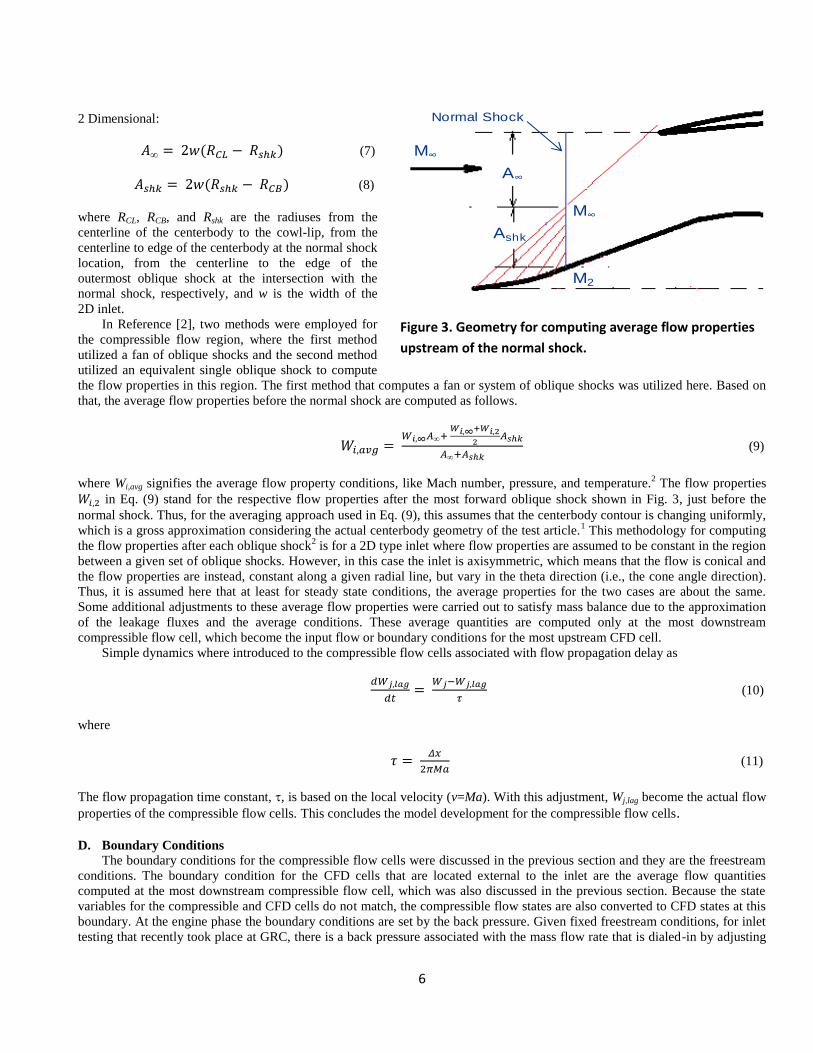
order to provide for the upstream boundary conditions of the adjacent quasi 1D computational domain. A depiction of this

compressible flow region is shown in Fig. 3. As shown in this figure, the flow properties at the normal shock boundary need to

be averaged with respect to the areas shown, in order to obtain a single value of averaged flow properties for the boundary

conditions of the CFD domain starting with the shock, down to the cowl-lip. This means that for the oblique shock system, these

flow properties would need to be averaged and then averaged again against the freestream flow properties according to these

areas. For axisymmetric and for 2 dimensional inlet geometries these areas can be computed as

Axisymmetric:

∞

(5)

(6)

Figure 2. Inlet capture versus inlet effective capture areas

and leakage mass flow rates.

6

2 Dimensional:

∞ (7)

(8)

where RCL, RCB, and Rshk are the radiuses from the

centerline of the centerbody to the cowl-lip, from the

centerline to edge of the centerbody at the normal shock

location, from the centerline to the edge of the

outermost oblique shock at the intersection with the

normal shock, respectively, and w is the width of the

2D inlet.

In Reference [2], two methods were employed for

the compressible flow region, where the first method

utilized a fan of oblique shocks and the second method

utilized an equivalent single oblique shock to compute

the flow properties in this region. The first method that computes a fan or system of oblique shocks was utilized here. Based on

that, the average flow properties before the normal shock are computed as follows.

∞

∞ (9)

where Wi,avg signifies the average flow property conditions, like Mach number, pressure, and temperature.2 The flow properties

in Eq. (9) stand for the respective flow properties after the most forward oblique shock shown in Fig. 3, just before the

normal shock. Thus, for the averaging approach used in Eq. (9), this assumes that the centerbody contour is changing uniformly,

which is a gross approximation considering the actual centerbody geometry of the test article.1 This methodology for computing

the flow properties after each oblique shock2 is for a 2D type inlet where flow properties are assumed to be constant in the region

between a given set of oblique shocks. However, in this case the inlet is axisymmetric, which means that the flow is conical and

the flow properties are instead, constant along a given radial line, but vary in the theta direction (i.e., the cone angle direction).

Thus, it is assumed here that at least for steady state conditions, the average properties for the two cases are about the same.

Some additional adjustments to these average flow properties were carried out to satisfy mass balance due to the approximation

of the leakage fluxes and the average conditions. These average quantities are computed only at the most downstream

compressible flow cell, which become the input flow or boundary conditions for the most upstream CFD cell.

Simple dynamics where introduced to the compressible flow cells associated with flow propagation delay as

(10)

where

(11)

The flow propagation time constant, , is based on the local velocity (v=Ma). With this adjustment, Wj,lag become the actual flow

properties of the compressible flow cells. This concludes the model development for the compressible flow cells.

D. Boundary Conditions

The boundary conditions for the compressible flow cells were discussed in the previous section and they are the freestream

conditions. The boundary condition for the CFD cells that are located external to the inlet are the average flow quantities

computed at the most downstream compressible flow cell, which was also discussed in the previous section. Because the state

variables for the compressible and CFD cells do not match, the compressible flow states are also converted to CFD states at this

boundary. At the engine phase the boundary conditions are set by the back pressure. Given fixed freestream conditions, for inlet

testing that recently took place at GRC, there is a back pressure associated with the mass flow rate that is dialed-in by adjusting

Figure 3. Geometry for computing average flow properties

upstream of the normal shock.

M∞

M∞

M2

A∞

Ashk

Normal Shock

7

the plug position at the inlet exit. Thus, the back pressure becomes the boundary condition at the engine face, and the inlet test

data were utilized to estimate the leakage mass flow rate and associated fluxes based on Eqs. (3) – (4). Thus, the leakage mass

flow rate as a function of back pressure also becomes a boundary condition for the external CFD cells. The remaining states at

the exit boundary can be computed by utilizing the following characteristic equation:2

(12)

To integrate the inlet to the existing engine simulations,4,5,6

the mass flow rate demand of the engine needs to be specified as a

boundary condition. However, it is not possible to directly use this boundary condition for the inlet model by itself. The reason is

that given the mass flow rate and the exit area, the solution to the relation for the density and velocity is non-

deterministic. This problem can be mitigated (see Ref. [2]) when the engine is integrated because given the mass flow rate and

engine speed the pressure ratio at the engine face can be determined. With the inlet by itself, this problem can be mitigated by

establishing a finite dynamic volume at the inlet exit that accepts the mass flow rate, similar to the way fluidic volumes are

modeled in Ref. [4]. By utilizing this latter approach, the mass flow demand at the inlet can be used with Eq. (3) to calculate the

leakage mass flow rate, thereby, removing the necessity of relying on test data for modeling the 1D flow of external compression

inlets.

E. Shock Sensing and Moving Computational Domains

The approach initially envisioned for separating the CFD and the compressible flow computational domains was to contract

CFD cells up to the most upstream shock position plus one more CFD cell. This would allow the shock to move one more cell

upstream under prevailing conditions at which time the most downstream compressible flow cell can be switched from

compressible flow to CFD. Similarly, this approach would also allow for downstream movement of the shock and appropriate

switching of cells between the two computational domains.

For the switching part, this is done by switching the derivatives between computational domains, which is appropriate since

no state variables are directly involved in the switching. However, the derivatives of the states interfacing the two computational

domains would need to be relative close to one another for simulation accuracy and for numerical stability. However, in terms of

knowing when exactly to switch interfacing cells of the two domains, accurate sensing of the shock position becomes an issue.

Also, accurately sensing when the shock actually wants to move, as opposed to movement due to normal shock gyrations,

becomes another issue.

In terms of sensing the shock position, the difficulty is that the shock is not exactly a vertical line. Rather, the shock spans

several cells, which starts with smoothly increasing pressure (or drop in Mach number). Then the shock pressure undergoes a

sharper rise towards the middle of the shock, followed by again a smoother tapering off. In addition, the shock strength decreases

as the shock moves towards the cowl-lip and the operation of the inlet under such conditions moves closer to isentropic. Thus,

where exactly the shock begins and where it ends is not as easy to detect. To alleviate this difficulty, the shock sensing method

was chosen to amplify the properties that identify the shock. Two alternative methods were employed where a shock sensing

property is constructed as

or (13)

Then the logic for shock detection at a given CFD cell is when the quantity exceeds a selected threshold. Examining Eq. (13),

it can be seen that the second option has higher sensitivity for shock sensing (logic protection was used for M=1). However, this

option was only briefly tested due to time limitations.

The second issue is how to detect that the shock is actually moving. If the shock moves upstream to the last CFD cell for

instance, this could imply that the shock is actually moving upstream. However, this can also be caused by shock gyrations, like

asymmetrical change in the flow properties or deviations in local artificial viscosity. Wrongly switching a compressible flow cell

to CFD could initiate a cascading movement of the shock in the upstream direction. This is because by wrongly removing a

compressible flow cell, this can cause the boundary pressure to the CFD domain to drop reciprocally. This cascading effect

would be more pronounced with the first method described above for estimating flux leakages by the compounding effect of

overestimating these flux leakages. A potential solution that is implemented for this problem is to allow appropriate switching of

cells interfacing these computational domains to occur only when movement is detected in the same direction and at the same

time on both trailing edges of the shock.

8

The process of cell switching is expected to introduce dynamics. However, the switching takes place within a single time

step and therefore, it would be expected that such dynamics will be well above the frequencies of interest. In terms of the physics

of the process, some dynamics could exist in this case as the shock movement would be expected to cause flow transition in this

region (in and out of compressible or conical flow). However, for the time spent on this problem, it cannot be said with certainty

that all the issues associated with this complex problem have been resolved and the solution has been generalized. That is, the

issues associated with accurately sensing the shock location, sensing shock movement, together with appropriate switching logic

for these moving computational domains and generalization of the problem to apply to any external compression inlet.

III. Simulation Results

As discussed earlier, the external compression inlet model with the first method for estimating the flux leakages was

simulated but so far the simulation did not behave as it would have been expected. This was primarily due to so far unresolved

issues with the method that resulted in overestimating the flux leakages. This caused the shock to cascade upstream to the nose

of the centerbody cone, independent of back pressure.

The second approach discussed before was simulated next, which produced acceptable results. This method provides for the

flux leakages based on estimating the mass flow rate spillage as the difference of the mass flow rate captured at the freestream

minus that flowing into the inlet. However, in this case a more damped viscosity coefficient was selected compared to the mixed

compression inlet (i.e., approximately 2.0 compared to 0.05 in Ref. [2]), which provides for more damping for the shock and also

prevents the build-up error from causing divergence in the solution space. The need to increase the viscosity coefficient to

provide for more damping may be a consequence of faster external dynamics. The penalty for increased damping may be that the

shock becomes more smeared compared to test results (i.e., the shock location occupying more cells than the shock in the

testing).

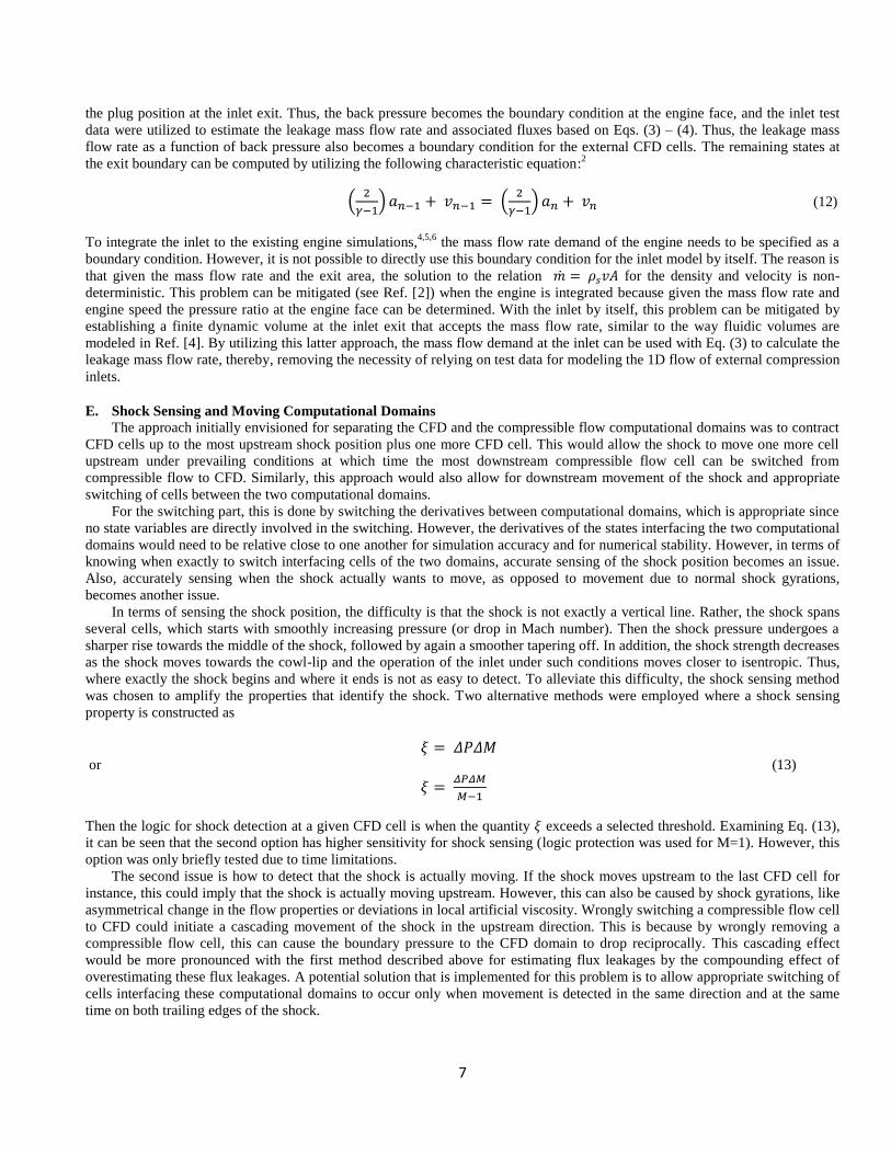
The first series of simulations conducted involved back pressure ramping to see if the shock movement followed expected

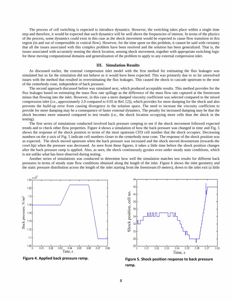
trends and to check other flow properties. Figure 4 shows a simulation of how the back pressure was changed in time and Fig. 5

shows the response of the shock position in terms of the most upstream CFD cell number that the shock occupies. Decreasing

numbers on the y-axis of Fig. 5 indicate cell numbers closer to the centerbody nose cone. The response of the shock position was

as expected. The shock moved upstream when the back pressure was increased and the shock moved downstream (towards the

cowl-lip) when the pressure was decreased. As seen from these figures, it takes a little time before the shock position changes

after the back pressure ramp is applied. Also, as seen, the shock continuously gyrates even under steady state conditions, which

is not unlike what has been observed during testing.

Another series of simulations was conducted to determine how well the simulation matches test results for different back

pressures in terms of steady state flow conditions obtained along the length of the inlet. Figure 6 shows the inlet geometry and

the static pressure distribution across the length of the inlet starting from the freestream (0 meters), down to the inlet exit (a little

Figure 5. Shock position response to back pressure

ramp.

Figure 4. Applied back pressure ramp.

9

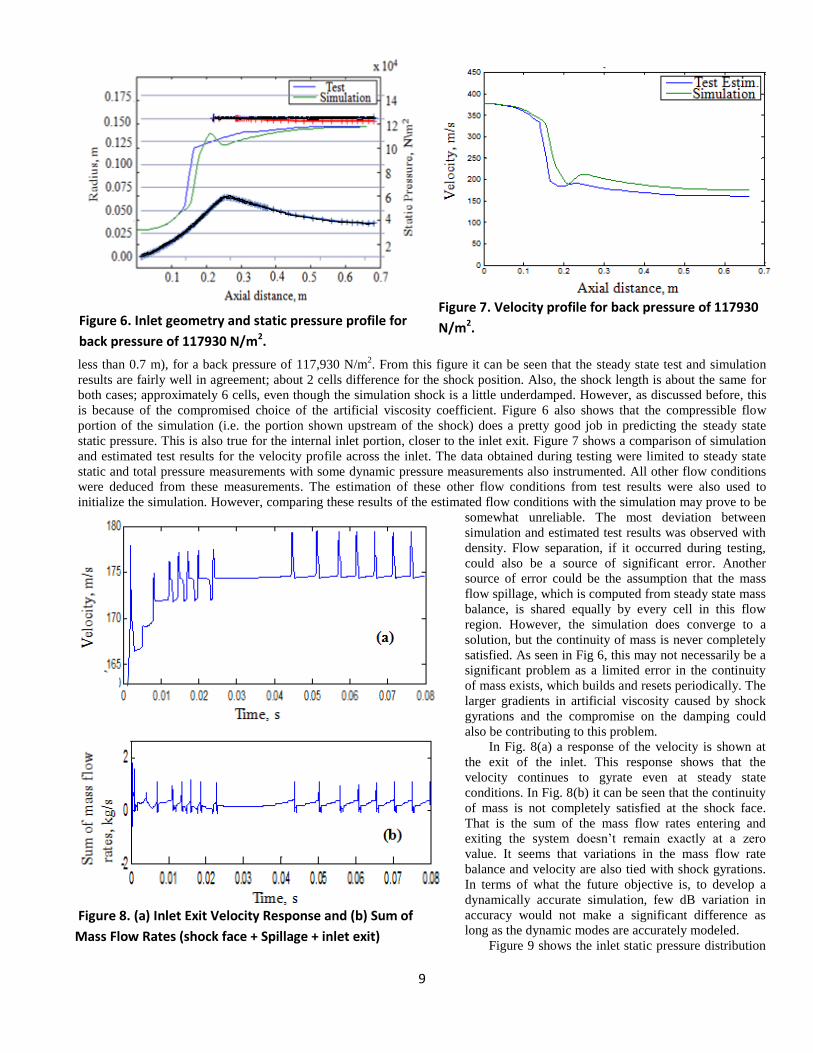
less than 0.7 m), for a back pressure of 117,930 N/m2. From this figure it can be seen that the steady state test and simulation

results are fairly well in agreement; about 2 cells difference for the shock position. Also, the shock length is about the same for

both cases; approximately 6 cells, even though the simulation shock is a little underdamped. However, as discussed before, this

is because of the compromised choice of the artificial viscosity coefficient. Figure 6 also shows that the compressible flow

portion of the simulation (i.e. the portion shown upstream of the shock) does a pretty good job in predicting the steady state

static pressure. This is also true for the internal inlet portion, closer to the inlet exit. Figure 7 shows a comparison of simulation

and estimated test results for the velocity profile across the inlet. The data obtained during testing were limited to steady state

static and total pressure measurements with some dynamic pressure measurements also instrumented. All other flow conditions

were deduced from these measurements. The estimation of these other flow conditions from test results were also used to

initialize the simulation. However, comparing these results of the estimated flow conditions with the simulation may prove to be

somewhat unreliable. The most deviation between

simulation and estimated test results was observed with

density. Flow separation, if it occurred during testing,

could also be a source of significant error. Another

source of error could be the assumption that the mass

flow spillage, which is computed from steady state mass

balance, is shared equally by every cell in this flow

region. However, the simulation does converge to a

solution, but the continuity of mass is never completely

satisfied. As seen in Fig 6, this may not necessarily be a

significant problem as a limited error in the continuity

of mass exists, which builds and resets periodically. The

larger gradients in artificial viscosity caused by shock

gyrations and the compromise on the damping could

also be contributing to this problem.

In Fig. 8(a) a response of the velocity is shown at

the exit of the inlet. This response shows that the

velocity continues to gyrate even at steady state

conditions. In Fig. 8(b) it can be seen that the continuity

of mass is not completely satisfied at the shock face.

That is the sum of the mass flow rates entering and

exiting the system doesn’t remain exactly at a zero

value. It seems that variations in the mass flow rate

balance and velocity are also tied with shock gyrations.

In terms of what the future objective is, to develop a

dynamically accurate simulation, few dB variation in

accuracy would not make a significant difference as

long as the dynamic modes are accurately modeled.

Figure 9 shows the inlet static pressure distribution

Figure 6. Inlet geometry and static pressure profile for

back pressure of 117930 N/m2.

Figure 7. Velocity profile for back pressure of 117930

N/m2.

Figure 8. (a) Inlet Exit Velocity Response and (b) Sum of

Mass Flow Rates (shock face + Spillage + inlet exit)

10

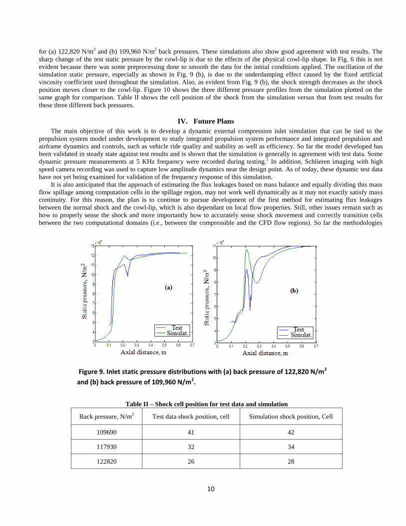
for (a) 122,820 N/m2 and (b) 109,960 N/m

2 back pressures. These simulations also show good agreement with test results. The

sharp change of the test static pressure by the cowl-lip is due to the effects of the physical cowl-lip shape. In Fig. 6 this is not

evident because there was some preprocessing done to smooth the data for the initial conditions applied. The oscillation of the

simulation static pressure, especially as shown in Fig. 9 (b), is due to the underdamping effect caused by the fixed artificial

viscosity coefficient used throughout the simulation. Also, as evident from Fig. 9 (b), the shock strength decreases as the shock

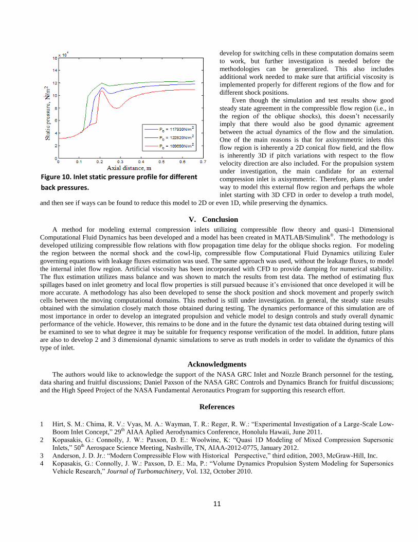
position moves closer to the cowl-lip. Figure 10 shows the three different pressure profiles from the simulation plotted on the

same graph for comparison. Table II shows the cell position of the shock from the simulation versus that from test results for

these three different back pressures.

IV. Future Plans

The main objective of this work is to develop a dynamic external compression inlet simulation that can be tied to the

propulsion system model under development to study integrated propulsion system performance and integrated propulsion and

airframe dynamics and controls, such as vehicle ride quality and stability as well as efficiency. So far the model developed has

been validated in steady state against test results and is shown that the simulation is generally in agreement with test data. Some

dynamic pressure measurements at 5 KHz frequency were recorded during testing.1 In addition, Schlieren imaging with high

speed camera recording was used to capture low amplitude dynamics near the design point. As of today, these dynamic test data

have not yet being examined for validation of the frequency response of this simulation.

It is also anticipated that the approach of estimating the flux leakages based on mass balance and equally dividing this mass

flow spillage among computation cells in the spillage region, may not work well dynamically as it may not exactly satisfy mass

continuity. For this reason, the plan is to continue to pursue development of the first method for estimating flux leakages

between the normal shock and the cowl-lip, which is also dependant on local flow properties. Still, other issues remain such as

how to properly sense the shock and more importantly how to accurately sense shock movement and correctly transition cells

between the two computational domains (i.e., between the compressible and the CFD flow regions). So far the methodologies

Figure 9. Inlet static pressure distributions with (a) back pressure of 122,820 N/m2

and (b) back pressure of 109,960 N/m2.

Table II – Shock cell position for test data and simulation

Back pressure, N/m2 Test data shock position, cell Simulation shock position, Cell

109690 41 42

117930 32 34

122820 26 28

11

develop for switching cells in these computation domains seem

to work, but further investigation is needed before the

methodologies can be generalized. This also includes

additional work needed to make sure that artificial viscosity is

implemented properly for different regions of the flow and for

different shock positions.

Even though the simulation and test results show good

steady state agreement in the compressible flow region (i.e., in

the region of the oblique shocks), this doesn’t necessarily

imply that there would also be good dynamic agreement

between the actual dynamics of the flow and the simulation.

One of the main reasons is that for axisymmetric inlets this

flow region is inherently a 2D conical flow field, and the flow

is inherently 3D if pitch variations with respect to the flow

velocity direction are also included. For the propulsion system

under investigation, the main candidate for an external

compression inlet is axisymmetric. Therefore, plans are under

way to model this external flow region and perhaps the whole

inlet starting with 3D CFD in order to develop a truth model,

and then see if ways can be found to reduce this model to 2D or even 1D, while preserving the dynamics.

V. Conclusion

A method for modeling external compression inlets utilizing compressible flow theory and quasi-1 Dimensional

Computational Fluid Dynamics has been developed and a model has been created in MATLAB/Simulink®. The methodology is

developed utilizing compressible flow relations with flow propagation time delay for the oblique shocks region. For modeling

the region between the normal shock and the cowl-lip, compressible flow Computational Fluid Dynamics utilizing Euler

governing equations with leakage fluxes estimation was used. The same approach was used, without the leakage fluxes, to model

the internal inlet flow region. Artificial viscosity has been incorporated with CFD to provide damping for numerical stability.

The flux estimation utilizes mass balance and was shown to match the results from test data. The method of estimating flux

spillages based on inlet geometry and local flow properties is still pursued because it’s envisioned that once developed it will be

more accurate. A methodology has also been developed to sense the shock position and shock movement and properly switch

cells between the moving computational domains. This method is still under investigation. In general, the steady state results

obtained with the simulation closely match those obtained during testing. The dynamics performance of this simulation are of

most importance in order to develop an integrated propulsion and vehicle model to design controls and study overall dynamic

performance of the vehicle. However, this remains to be done and in the future the dynamic test data obtained during testing will

be examined to see to what degree it may be suitable for frequency response verification of the model. In addition, future plans

are also to develop 2 and 3 dimensional dynamic simulations to serve as truth models in order to validate the dynamics of this

type of inlet.

Acknowledgments

The authors would like to acknowledge the support of the NASA GRC Inlet and Nozzle Branch personnel for the testing,

data sharing and fruitful discussions; Daniel Paxson of the NASA GRC Controls and Dynamics Branch for fruitful discussions;

and the High Speed Project of the NASA Fundamental Aeronautics Program for supporting this research effort.

References

1 Hirt, S. M.: Chima, R. V.: Vyas, M. A.: Wayman, T. R.: Reger, R. W.: “Experimental Investigation of a Large-Scale Low-

Boom Inlet Concept,” 29th

AIAA Aplied Aerodynamics Conference, Honolulu Hawaii, June 2011.

2 Kopasakis, G.: Connolly, J. W.: Paxson, D. E.: Woolwine, K: “Quasi 1D Modeling of Mixed Compression Supersonic

Inlets,” 50th

Aerospace Science Meeting, Nashville, TN, AIAA-2012-0775, January 2012.

3 Anderson, J. D. Jr.: “Modern Compressible Flow with Historical Perspective,” third edition, 2003, McGraw-Hill, Inc.

4 Kopasakis, G.: Connolly, J. W.: Paxson, D. E.: Ma, P.: “Volume Dynamics Propulsion System Modeling for Supersonics

Vehicle Research,” Journal of Turbomachinery, Vol. 132, October 2010.

Figure 10. Inlet static pressure profile for different

back pressures.

12

5 Connolly, J.: Kopasakis, G.: Lemon, K.: “Turbofan Volume Dynamics Model for Investigations of Aero-Propulso-Servo-

Elastic Effects in a Supersonic Commercial Transport”, 46th

AIAA/ASME/SAE/ASEE Joint Propulsion Conference and

Exhibit, AIAA-2009-4802, August, 2009.

6 Connolly, J.: Kopasakis, G.: Paxson, D.: Stuber, E.: Woolwine, K.: “Nonlinear Dynamic Modeling and Controls

Development for Supersonic Propulsion System Research,” 48th

AIAA/ASME/SAE/ASEE Joint Propulsion Conference and

Exhibit, AIAA 2011-5635, August, 2011.

7 Lassaux, G.: “High-Fidelity Reduced-Order Aerodynamic Models: Application to Active Control of Engine Inlets,”

Master’s thesis, Dept. of Aeronautics and Astronautics, MIT, Cambridge, MA, June 2002.

8 Lassaux, G.: Willcox, K.: “Model reduction for active control design using multiple-point Arnoldi methods,” AIAA

Aerospace Sciences Meeting& Exhibit, Reno, NV, AIAA-2003-616, January 2003.

9 Willcox, K.: Megretski, A.: “Fourier Series for Accurate, Stable, Reduced-Order Models for Linear CFD Applications,”

AIAA Computational Fluid Dynamics Conference, Orlando, FL, AIAA-2003-4235, June, 2003.

10 Chicatelli, A.: Hartley, T. T.: “A Method for Generating Reduced-Order Linear Models of Multidimensional Supersonic

Inlets,” NASA CR-1998-207405.

11 Varner, M.O., Martindale, W.J. Phares, K.R, Kneile, K.R., Adams, J.C., “Large Perturbation Flow Field Analysis and

Simulation for Supersonic Inlets Final Report,” NASA CR 174676

12 Moeckel, W.E., “Approximate Method for Predicting Form and Location of Detached Shock Waves Ahead of Place or

Axially Symmetric Bodies,” NASA TN-1921