Query Processing and Optimization

Query processing Overview The activities involved in retrieving data from the

database. Query processing is the procedure of transforming a

high level query (SQL) into correct and efficient execution plan expressed in low level language that perform requires retrieval and manipulations in the d/b.

There are four main phases of query processing: Decompostion Optimization Code Generation Execution

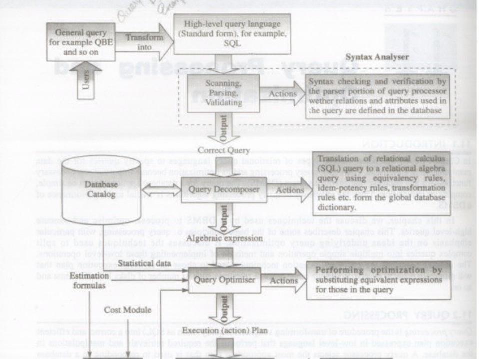
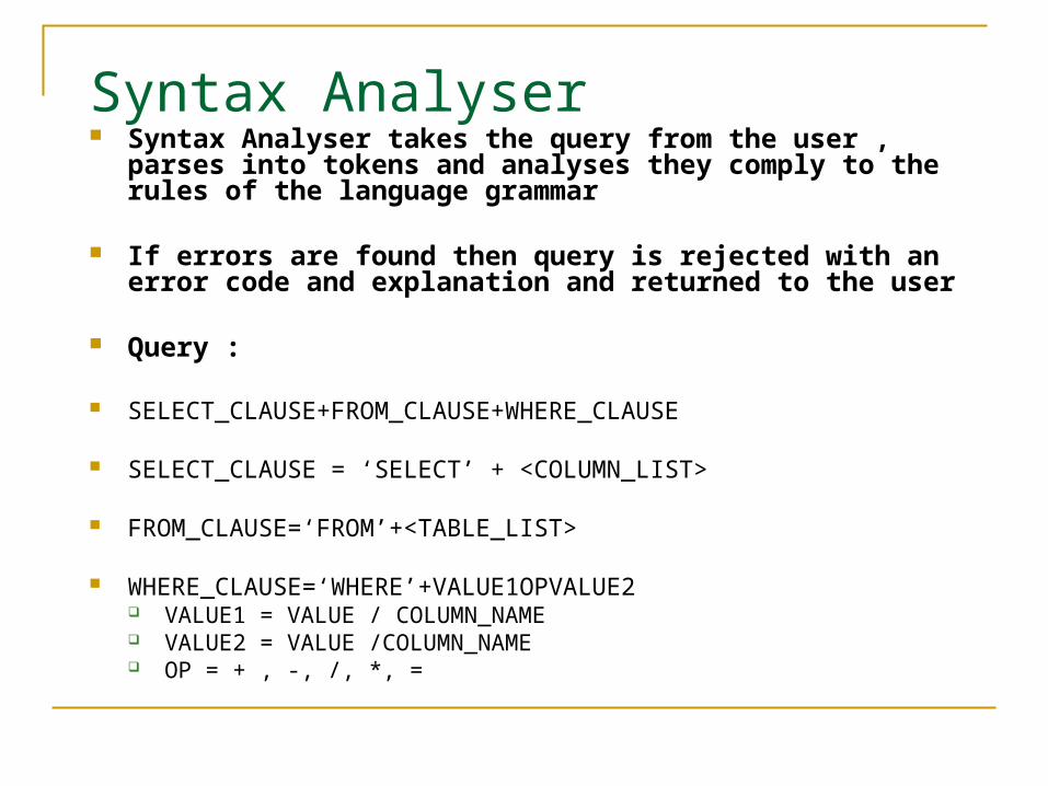
Syntax Analyser Syntax Analyser takes the query from the user , parses into

tokens and analyses they comply to the rules of the language grammar

If errors are found then query is rejected with an error code and explanation and returned to the user

Query :

SELECT_CLAUSE+FROM_CLAUSE+WHERE_CLAUSE

SELECT_CLAUSE = ‘SELECT’ + <COLUMN_LIST>

FROM_CLAUSE=‘FROM’+<TABLE_LIST>

WHERE_CLAUSE=‘WHERE’+VALUE1OPVALUE2 VALUE1 = VALUE / COLUMN_NAME VALUE2 = VALUE /COLUMN_NAME OP = + , -, /, *, =

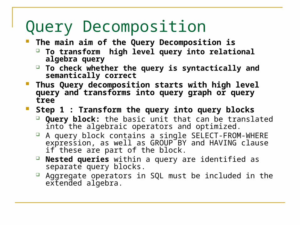
Query Decomposition The main aim of the Query Decomposition is

To transform high level query into relational algebra query

To check whether the query is syntactically and semantically correct

Thus Query decomposition starts with high level query and transforms into query graph or query tree

Step 1 : Transform the query into query blocks Query block: the basic unit that can be translated into the

algebraic operators and optimized. A query block contains a single SELECT-FROM-WHERE

expression, as well as GROUP BY and HAVING clause if these are part of the block.

Nested queries within a query are identified as separate query blocks.

Aggregate operators in SQL must be included in the extended algebra.

Query Decomposition

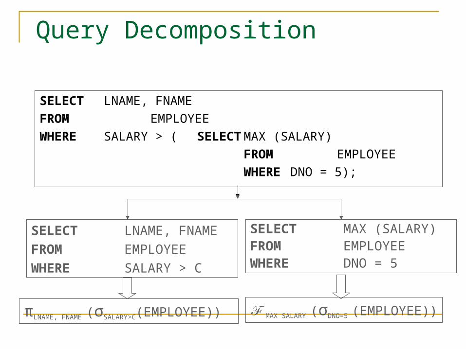
SELECT LNAME, FNAME

FROM EMPLOYEE

WHERE SALARY > ( SELECT MAX (SALARY)

FROM EMPLOYEE

WHERE DNO = 5);

SELECT MAX (SALARY)FROM EMPLOYEEWHERE DNO = 5

SELECT LNAME, FNAME

FROM EMPLOYEE

WHERE SALARY > C

πLNAME, FNAME (σSALARY>C(EMPLOYEE)) ℱMAX SALARY (σDNO=5 (EMPLOYEE))

Query Decomposition

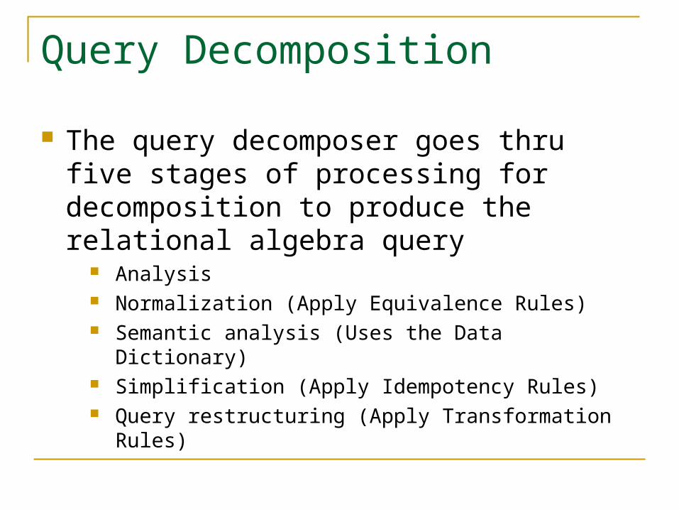
The query decomposer goes thru five stages of processing for decomposition to produce the relational algebra query

Analysis Normalization (Apply Equivalence Rules) Semantic analysis (Uses the Data Dictionary) Simplification (Apply Idempotency Rules) Query restructuring (Apply Transformation Rules)

Query Analysis

The query is lexically and syntactically analyzed using the techniques of programming language compilers.

Verifies that the relations and attributes specified in the query are defined in the system catalog.

Verifies that any operations applied to database objects are appropriate for the object type.

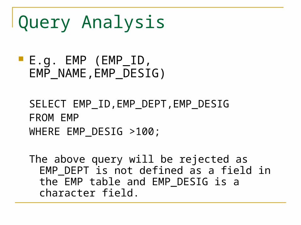
Query Analysis

E.g. EMP (EMP_ID, EMP_NAME,EMP_DESIG)

SELECT EMP_ID,EMP_DEPT,EMP_DESIGFROM EMPWHERE EMP_DESIG >100;

The above query will be rejected as EMP_DEPT is not defined as a field in the EMP table and EMP_DESIG is a character field.

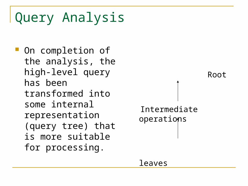
Query Analysis

On completion of the analysis, the high-level query has been transformed into some internal representation (query tree) that is more suitable for processing.

Root

Intermediate operations

leaves

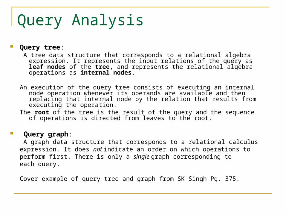
Query Analysis

Query tree: A tree data structure that corresponds to a relational algebra expression. It

represents the input relations of the query as leaf nodes of the tree, and represents the relational algebra operations as internal nodes.

An execution of the query tree consists of executing an internal node operation whenever its operands are available and then replacing that internal node by the relation that results from executing the operation.

The root of the tree is the result of the query and the sequence of operations is directed from leaves to the root.

Query graph: A graph data structure that corresponds to a relational calculusexpression. It does not indicate an order on which operations toperform first. There is only a single graph corresponding toeach query.

Cover example of query tree and graph from SK Singh Pg. 375.

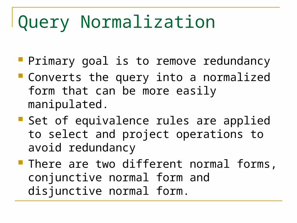
Query Normalization

Primary goal is to remove redundancy Converts the query into a normalized form

that can be more easily manipulated. Set of equivalence rules are applied to select

and project operations to avoid redundancy There are two different normal forms,

conjunctive normal form and disjunctive normal form.

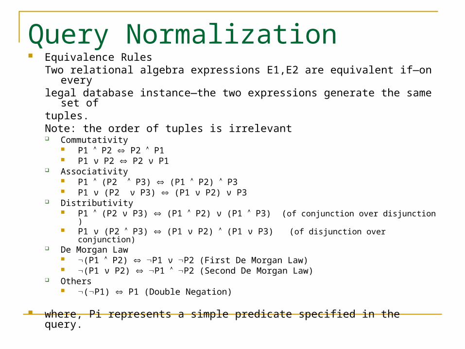
Query Normalization Equivalence Rules

Two relational algebra expressions E1,E2 are equivalent if—on everylegal database instance—the two expressions generate the same set oftuples.Note: the order of tuples is irrelevant Commutativity

P1 P2 P2 P1 P1 ν P2 P2 ν P1

Associativity P1 (P2 P3) (P1 P2) P3 P1 ν (P2 ν P3) (P1 ν P2) ν P3

Distributivity P1 (P2 ν P3) (P1 P2) ν (P1 P3) (of conjunction over disjunction ) P1 ν (P2 P3) (P1 ν P2) (P1 ν P3) (of disjunction over conjunction)

De Morgan Law (P1 P2) P1 ν P2 (First De Morgan Law) (P1 ν P2) P1 P2 (Second De Morgan Law)

Others (P1) P1 (Double Negation)

where, Pi represents a simple predicate specified in the query.

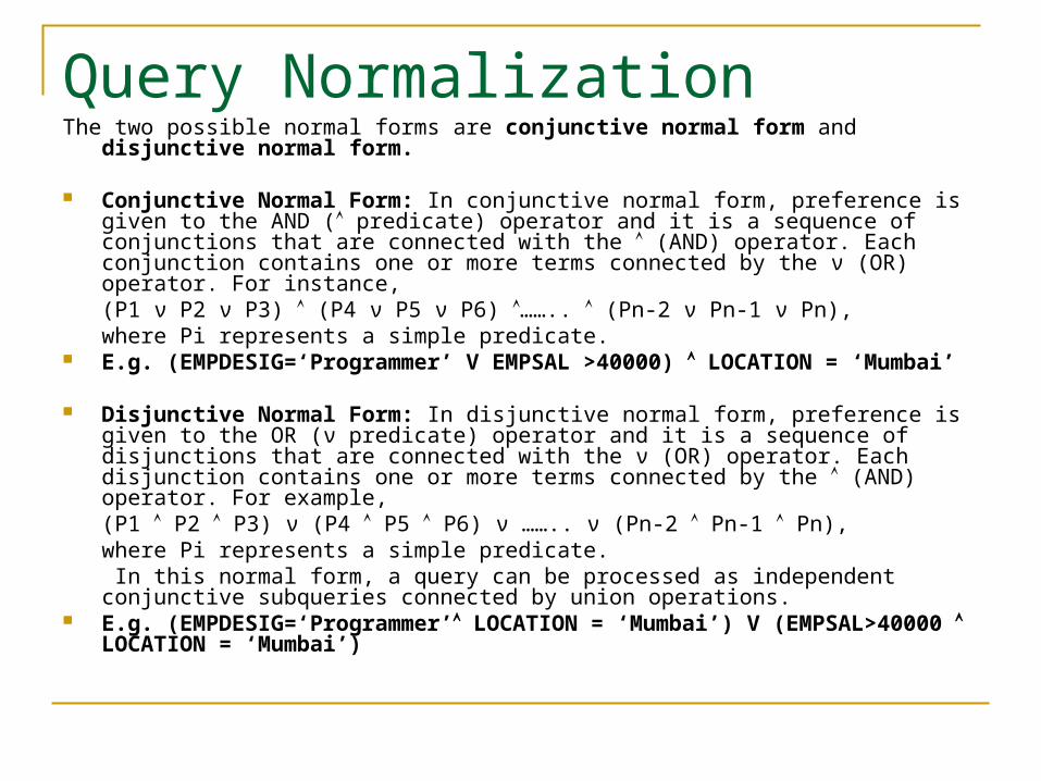
Query NormalizationThe two possible normal forms are conjunctive normal form and disjunctive normal form.

Conjunctive Normal Form: In conjunctive normal form, preference is given to the AND ( predicate) operator and it is a sequence of conjunctions that are connected with the (AND) operator. Each conjunction contains one or more terms connected by the ν (OR) operator. For instance,(P1 ν P2 ν P3) (P4 ν P5 ν P6) …….. (Pn-2 ν Pn-1 ν Pn),where Pi represents a simple predicate.

E.g. (EMPDESIG=‘Programmer’ V EMPSAL >40000) LOCATION = ‘Mumbai’

Disjunctive Normal Form: In disjunctive normal form, preference is given to the OR (ν predicate) operator and it is a sequence of disjunctions that are connected with the ν (OR) operator. Each disjunction contains one or more terms connected by the (AND) operator. For example,(P1 P2 P3) ν (P4 P5 P6) ν …….. ν (Pn-2 Pn-1 Pn),where Pi represents a simple predicate. In this normal form, a query can be processed as independent conjunctive subqueries connected by union operations.

E.g. (EMPDESIG=‘Programmer’ LOCATION = ‘Mumbai’) V (EMPSAL>40000 LOCATION = ‘Mumbai’)

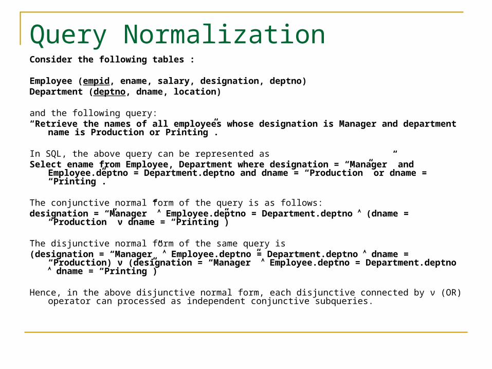
Query NormalizationConsider the following tables :

Employee (empid, ename, salary, designation, deptno)Department (deptno, dname, location)

and the following query:“Retrieve the names of all employees whose designation is Manager and department name is

Production or Printing”.

In SQL, the above query can be represented asSelect ename from Employee, Department where designation = “Manager” and Employee.deptno =

Department.deptno and dname = “Production” or dname = “Printing”.

The conjunctive normal form of the query is as follows:designation = “Manager” Employee.deptno = Department.deptno (dname = “Production” ν dname =

“Printing”)

The disjunctive normal form of the same query is(designation = “Manager” Employee.deptno = Department.deptno dname = “Production) ν

(designation = “Manager” Employee.deptno = Department.deptno dname = “Printing”)

Hence, in the above disjunctive normal form, each disjunctive connected by ν (OR) operator can processed as independent conjunctive subqueries.

Semantic analysis The objective is to reject normalized queries that are incorrectly

formulated or contradictory. The query is lexically and syntactically analyzed in this step by

using the compiler of high-level query language in which the query is expressed.

In addition, this step verifies whether the relations and attributes specified in the query are defined in the conceptual schema or not.

It is also checked in the analysis step that the operations to database objects specified in the given query are correct for the object type.

When one of the above incorrectness is detected, the query is returned to the user with an explanation; otherwise, the high-level query has been transformed into an internal form for further processing. The incorrectness in the query is detected based on the

corresponding query graph or relation connection graph A query is contradictory if its normalized attribute connection

graph contains a cycle for which the valuation sum is negative.

Semantic analysis Query graph or relation connection graph

A node is created in the query graph for the result and for each base relation specified in the query.

An edge between two nodes is drawn in the query graph for each join operation and for each project operation in the query. An edge between two nodes that are not result nodes represents a join operation, while an edge whose destination node is the result node represents a project operation.

A node in the query graph which is not result node is labeled by a select operation or a self-join operation specified in the query.

The relation connection graph is used to check the semantic correctness of the query. A query is semantically incorrect if its relation connection graph is not connected.

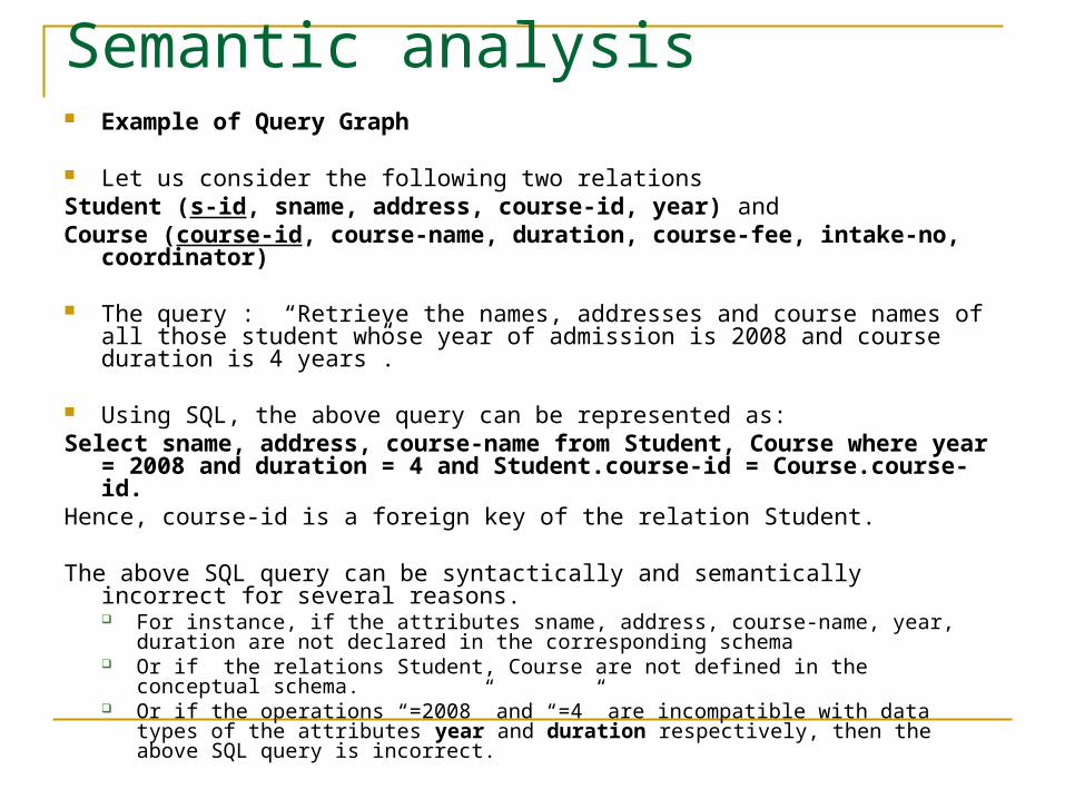
Semantic analysis Example of Query Graph

Let us consider the following two relationsStudent (s-id, sname, address, course-id, year) and Course (course-id, course-name, duration, course-fee, intake-no, coordinator)

The query : “Retrieve the names, addresses and course names of all those student whose year of admission is 2008 and course duration is 4 years”.

Using SQL, the above query can be represented as:Select sname, address, course-name from Student, Course where year = 2008

and duration = 4 and Student.course-id = Course.course-id. Hence, course-id is a foreign key of the relation Student.

The above SQL query can be syntactically and semantically incorrect for several reasons. For instance, if the attributes sname, address, course-name, year, duration are not

declared in the corresponding schema Or if the relations Student, Course are not defined in the conceptual schema. Or if the operations “=2008” and “=4” are incompatible with data types of the attributes

year and duration respectively, then the above SQL query is incorrect.

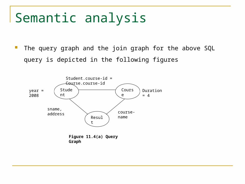
Semantic analysis

The query graph and the join graph for the above SQL query is depicted in

the following figures

Student

Course

Result

Duration = 4year = 2008

Student.course-id = Course.course-id

sname, address course-

name

Figure 11.4(a) Query Graph

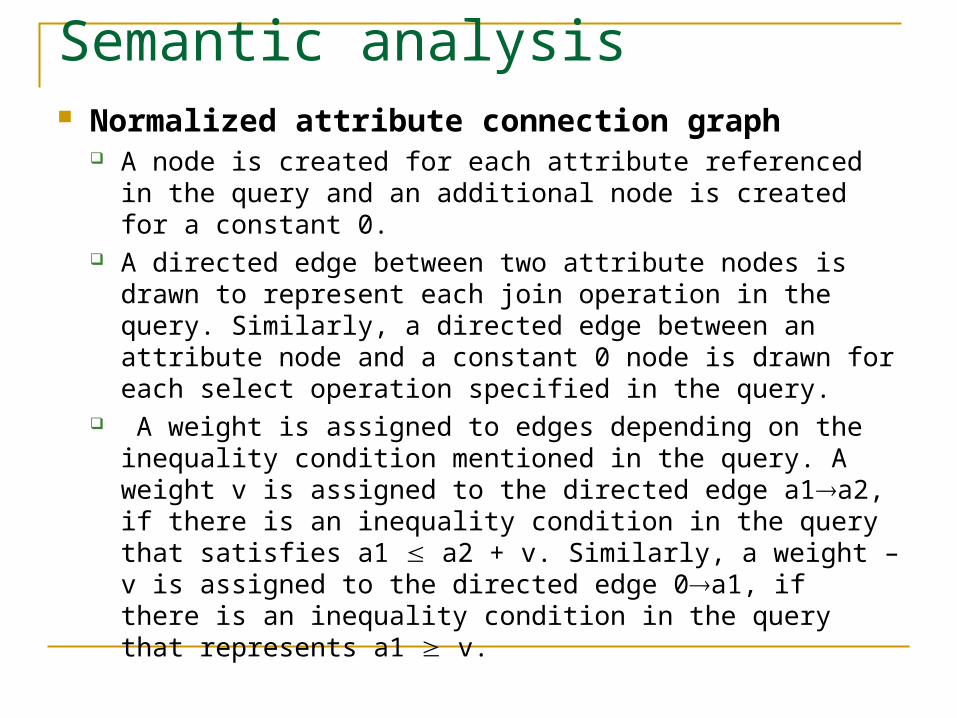
Semantic analysis Normalized attribute connection graph

A node is created for each attribute referenced in the query and an additional node is created for a constant 0.

A directed edge between two attribute nodes is drawn to represent each join operation in the query. Similarly, a directed edge between an attribute node and a constant 0 node is drawn for each select operation specified in the query.

A weight is assigned to edges depending on the inequality condition mentioned in the query. A weight v is assigned to the directed edge a1a2, if there is an inequality condition in the query that satisfies a1 a2 + v. Similarly, a weight –v is assigned to the directed edge 0a1, if there is an inequality condition in the query that represents a1 v.

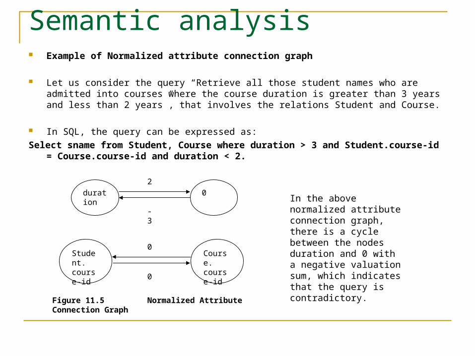
Semantic analysis Example of Normalized attribute connection graph

Let us consider the query “Retrieve all those student names who are admitted into courses where the course duration is greater than 3 years and less than 2 years”, that involves the relations Student and Course.

In SQL, the query can be expressed as:

Select sname from Student, Course where duration > 3 and Student.course-id = Course.course-id and duration < 2.

Figure 11.5 Normalized Attribute Connection Graph

duration

0

-3

2

Student.course-id

Course.course-id

0

0

In the above normalized attribute connection graph, there is a cycle between the nodes duration and 0 with a negative valuation sum, which indicates that the query is contradictory.

Simplification To detect redundant qualifications, eliminate common subexpressions , and

transform the query to a semantically equivalent but more easily and efficiently computed form.

Access restrictions, view definitions, and integrity constraints are considered at this stage.

If the query contradicts integrity constraints then it must be rejected, also if the user does not have appropriate access rights to all the components of the query, then it must be rejected.

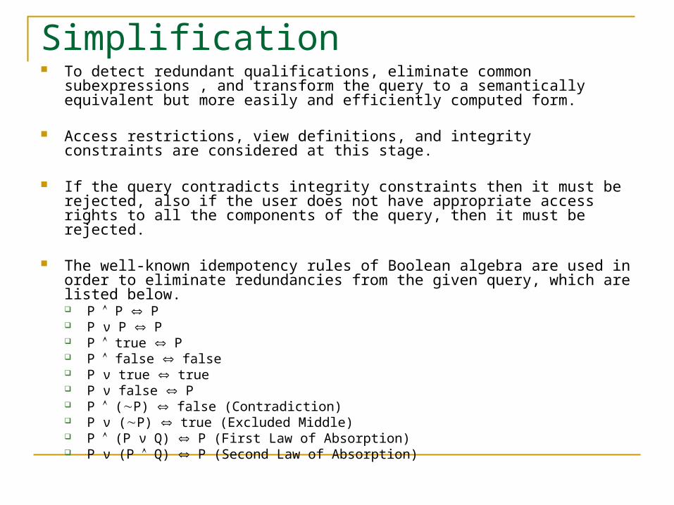
The well-known idempotency rules of Boolean algebra are used in order to eliminate redundancies from the given query, which are listed below. P P P P ν P P P true P P false false P ν true true P ν false P P (P) false (Contradiction) P ν (P) true (Excluded Middle) P (P ν Q) P (First Law of Absorption) P ν (P Q) P (Second Law of Absorption)

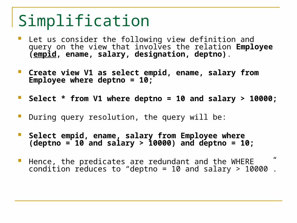
Simplification Let us consider the following view definition and query on the view that

involves the relation Employee (empid, ename, salary, designation, deptno).

Create view V1 as select empid, ename, salary from Employee where deptno = 10;

Select * from V1 where deptno = 10 and salary > 10000;

During query resolution, the query will be: Select empid, ename, salary from Employee where (deptno = 10

and salary > 10000) and deptno = 10;

Hence, the predicates are redundant and the WHERE condition reduces to “deptno = 10 and salary > 10000”.

Query restructuring In this step, the query in high-level language is rewritten into equivalent

relational algebraic form. This step involves two sub steps. Initially, the query is converted into equivalent relational algebraic form and then the relational algebraic query is restructured to improve performance. The relational algebraic query is represented by query tree or operator tree which can be constructed as follows:

A leaf node is created for each relation specified in the query. A non-leaf node is created for each intermediate relation in the query that

can be produced by a relational algebraic operation. The root of query tree represents the result of the query and the sequence of

operations is directed from the leaves to the root. In relational data model, the conversion from SQL query to relational

algebraic form can be done in an easier way. The leaf nodes in the query tree are created from the FROM clause of SQL query. The root node is created as a project operation involving the result attributes from the SELECT clause specified in SQL query. The sequence of relational algebraic operations, which depends on the WHERE clause of SQL query, is directed from leaves to the root of the query tree.

The derived query is now optimized using the Transformation Rules

Query optimization The activity of choosing an efficient execution strategy for

processing a query. An important aspect of query processing is query optimization. The aim of query optimization is to choose the one that

minimizes resource usage (I/O, CPU time) Every method of query optimization depend on database

statistics. The statistics cover information about relations, attribute, and

indexes. Keeping the statistics current can be problematic. If the DBMS updates the statistics every time a tuple is inserted,

updated, or deleted, this would have a significant impact on performance during peak period.

An alternative approach is to update the statistics on a periodic basis, for example nightly, or whenever the system is idle.

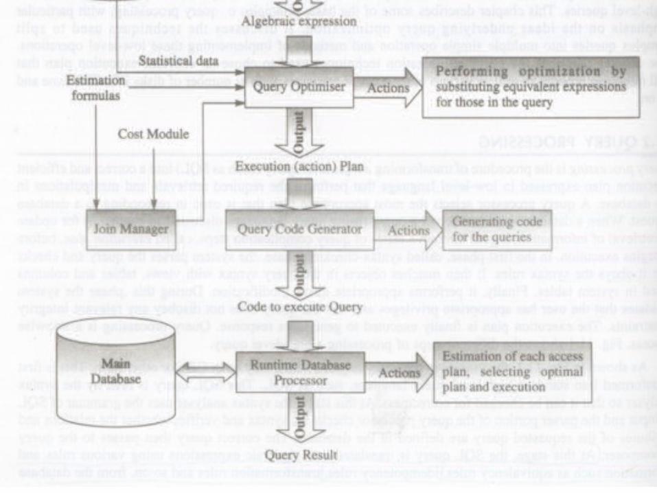
Query optimization Four main inputs for the Query Optimization

Relational Algebra Query (generated by the Query Decomposer)

Estimation formulas used to determine cardinality of intermediate results

A cost model Statistical data from the database catalogue

The output is the optimized query

Query Optimization 1. Why do we need to optimize?

A high-level relational query is generally non-procedural in nature.

It says “what", rather than “how" to find it. When a query is presented to the system, it is useful to find an

efficient method of finding the answer, using the existing database structure.

Usually worthwhile for the system to spend some time on strategy selection.

Typically can be done using information in main memory, with little or no disk access.

Execution of the query will require disk accesses. Transfer of data from disk is slow, relative to the speed of

main memory and the CPU It is advantageous to spend a considerable amount of

processing to save disk accesses

2. Do we really optimize?

Optimizing means finding the best of all possible methods.

The term “optimization" is a bit of a misnomer here. Usually the system does not calculate the cost of all

possible strategies. Perhaps “query improvement" is a better term.3. Two main approaches: (a) Rewriting the query in a more effective manner by

applying the Heuristic rules of optimization (b) Systematic estimation of the cost of various

execution strategies for the query and choosing the plan with the lowest cost estimate.

Transformation Rules or Equivalence rule Transformation rules are used by query

optimizer to transform one relational algebra expression into an equivalent expression that is more efficient to execute.

Relation is considered as equivalent of another relation if two relations have same set of attributes in a different order but representing the same information.

This rules are used to restructure the canonical (initial) relation algebra tree generated during query decomposition.

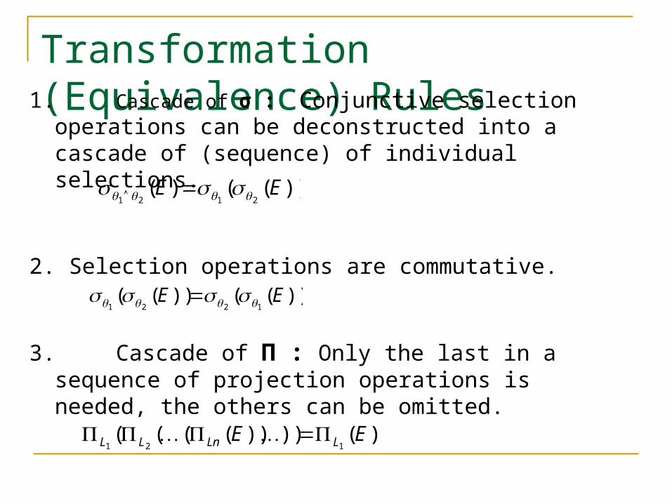
Transformation (Equivalence) Rules1. Cascade of σ : Conjunctive selection operations can

be deconstructed into a cascade of (sequence) of individual selections.

2. Selection operations are commutative.

3. Cascade of Π : Only the last in a sequence of projection operations is needed, the others can be omitted.

))(())((1221EE

))(()(2121EE

)())))((((121EE LLnLL

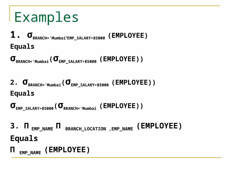
Examples1. σBRANCH=‘MumbaiEMP_SALARY>85000 (EMPLOYEE)

Equals

σBRANCH=‘Mumbai(σEMP_SALARY>85000 (EMPLOYEE))

2. σBRANCH=‘Mumbai(σEMP_SALARY>85000 (EMPLOYEE))

Equals

σEMP_SALARY>85000(σBRANCH=‘Mumbai (EMPLOYEE))

3. Π EMP_NAME Π BRANCH_LOCATION ,EMP_NAME (EMPLOYEE)

Equals

Π EMP_NAME (EMPLOYEE)

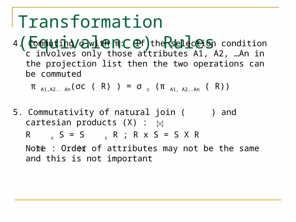
Transformation (Equivalence) Rules4. Commuting σ with π: If the selection condition c involves

only those attributes A1, A2, …An in the projection list then the two operations can be commuted

π A1,A2.. An(σc ( R) ) = σ c (π A1, A2..An ( R))

5. Commutativity of natural join ( ) and cartesian products (X) :

R c S = S c R ; R x S = S X R

Note : Order of attributes may not be the same and this is not important

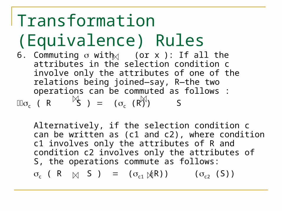
Transformation (Equivalence) Rules6. Commuting with (or x): If all the attributes

in the selection condition c involve only the attributes of one of the relations being joined—say, R—the two operations can be commuted as follows :

c ( R S ) (c (R)) S

Alternatively, if the selection condition c can be written as (c1 and c2), where condition c1 involves only the attributes of R and condition c2 involves only the attributes of S, the operations commute as follows:

c ( R S ) (c1 (R)) (c2 (S))

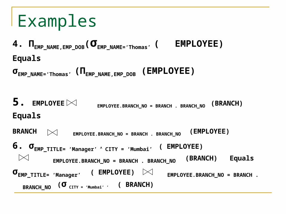
Examples4. ΠEMP_NAME,EMP_DOB(σEMP_NAME=‘Thomas’ ( EMPLOYEE)

Equals

σEMP_NAME=‘Thomas’ (ΠEMP_NAME,EMP_DOB (EMPLOYEE)

5. EMPLOYEE EMPLOYEE.BRANCH_NO = BRANCH . BRANCH_NO (BRANCH)

Equals

BRANCH EMPLOYEE.BRANCH_NO = BRANCH . BRANCH_NO (EMPLOYEE)

6. σEMP_TITLE= ‘Manager’ CITY = ‘Mumbai’ ( EMPLOYEE)

EMPLOYEE.BRANCH_NO = BRANCH . BRANCH_NO (BRANCH) Equals

σEMP_TITLE= ‘Manager’ ( EMPLOYEE) EMPLOYEE.BRANCH_NO = BRANCH .

BRANCH_NO (σ CITY = ‘Mumbai’ ’ ( BRANCH)

Equivalence Rules (Cont.)7. Commuting with (or x): Suppose that the

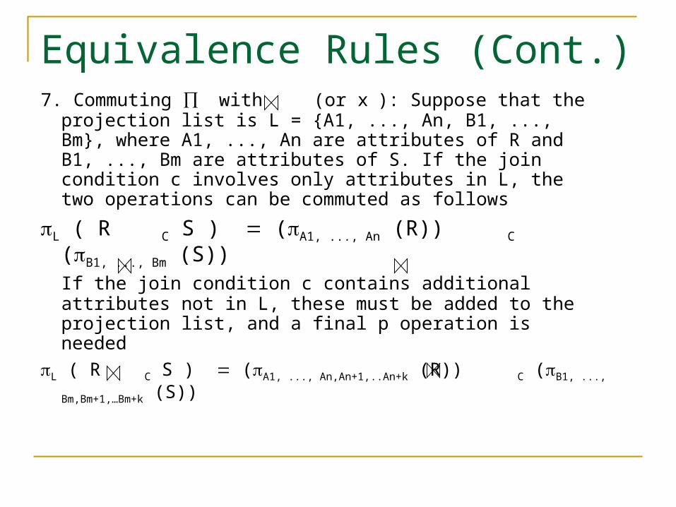
projection list is L = {A1, ..., An, B1, ..., Bm}, where A1, ..., An are attributes of R and B1, ..., Bm are attributes of S. If the join condition c involves only attributes in L, the two operations can be commuted as follows

L ( R C S ) (A1, ..., An (R)) C (B1, ..., Bm (S)) If the join condition c contains additional attributes not in L, these must be added to the projection list, and a final p operation is needed

L ( R C S ) (A1, ..., An,An+1,..An+k (R)) C (B1, ..., Bm,Bm+1,…

Bm+k (S))

Equivalence Rules (Cont.)

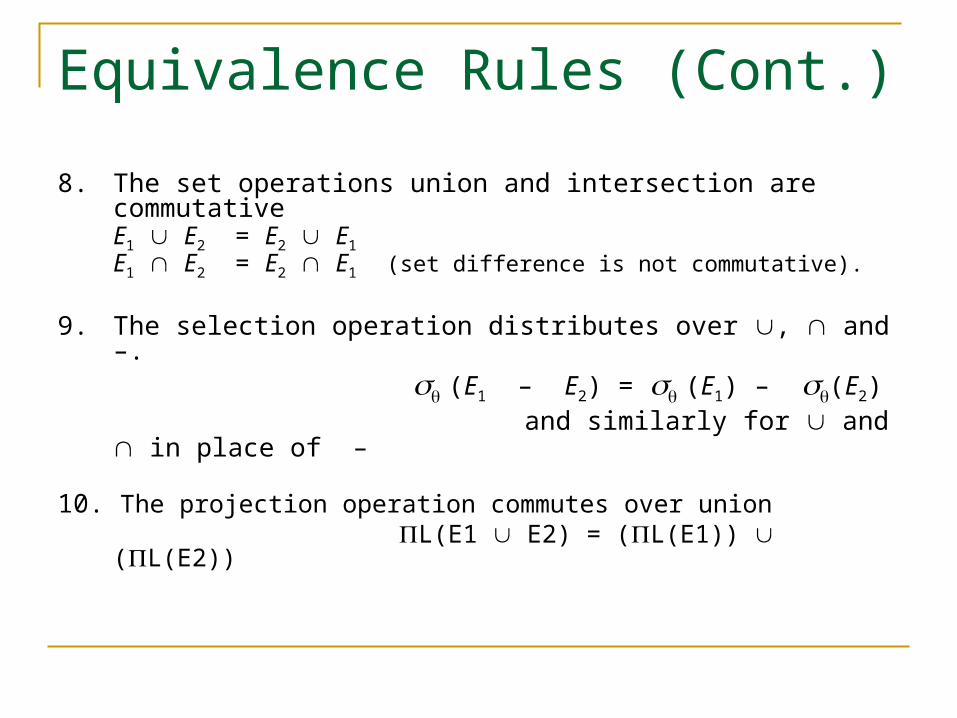
8. The set operations union and intersection are commutative E1 E2 = E2 E1 E1 E2 = E2 E1 (set difference is not commutative).

9. The selection operation distributes over , and –. (E1 – E2) = (E1) – (E2) and similarly for and in place of –

10. The projection operation commutes over union L(E1 E2) = (L(E1)) (L(E2))

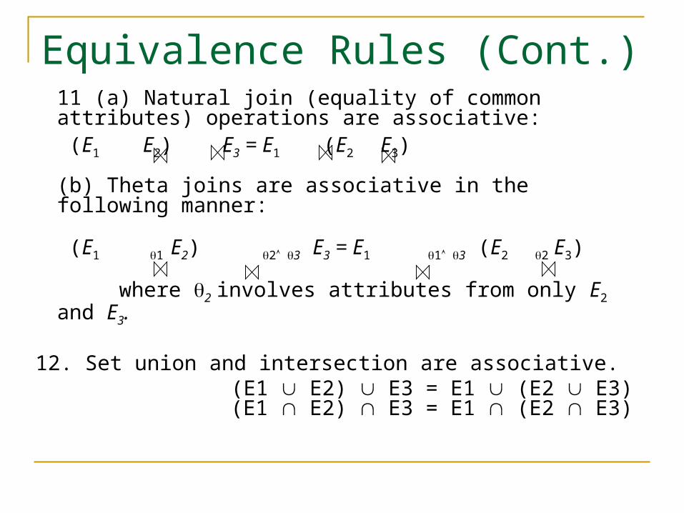
Equivalence Rules (Cont.)11 (a) Natural join (equality of common attributes) operations are associative:

(E1 E2) E3 = E1 (E2 E3)

(b) Theta joins are associative in the following manner:

(E1 1 E2) 2 3 E3 = E1 1 3 (E2 2 E3) where 2 involves attributes from only E2 and E3.

12. Set union and intersection are associative. (E1 E2) E3 = E1 (E2 E3) (E1 E2) E3 = E1 (E2 E3)

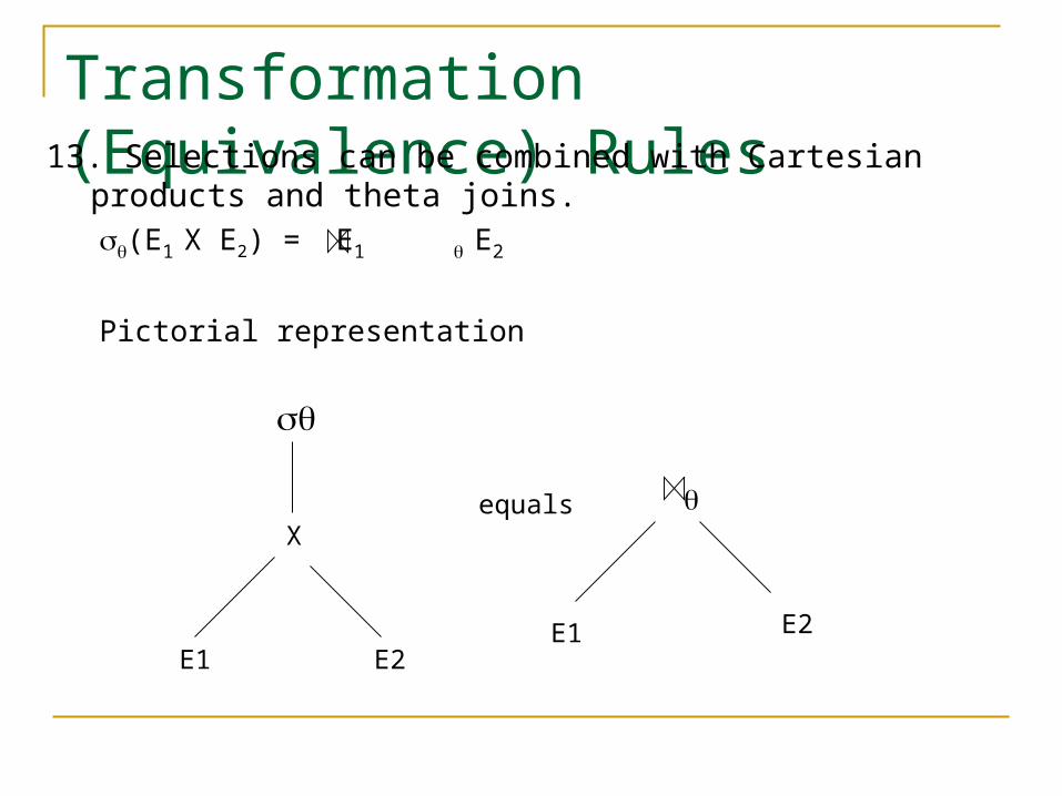
Transformation (Equivalence) Rules13. Selections can be combined with Cartesian products and

theta joins.(E1 X E2) = E1 E2

Pictorial representation

E1 E2

X

equals

E1 E2

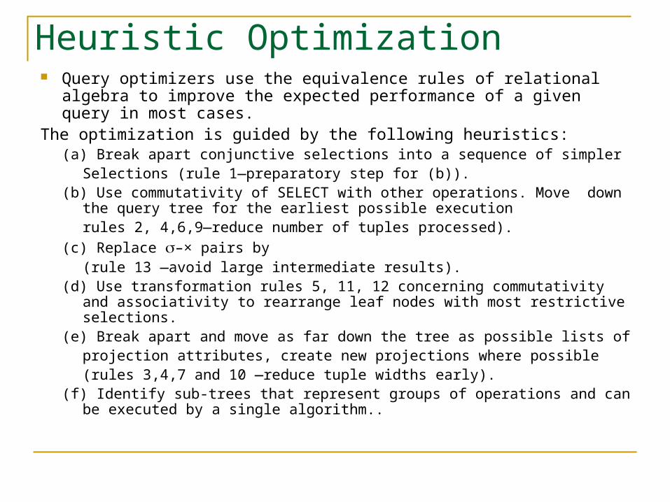
Heuristic Optimization Query optimizers use the equivalence rules of relational algebra to

improve the expected performance of a given query in most cases.The optimization is guided by the following heuristics:

(a) Break apart conjunctive selections into a sequence of simplerSelections (rule 1—preparatory step for (b)).

(b) Use commutativity of SELECT with other operations. Move down the query tree for the earliest possible executionrules 2, 4,6,9—reduce number of tuples processed).

(c) Replace –× pairs by (rule 13 —avoid large intermediate results).

(d) Use transformation rules 5, 11, 12 concerning commutativity and associativity to rearrange leaf nodes with most restrictive selections.

(e) Break apart and move as far down the tree as possible lists ofprojection attributes, create new projections where possible(rules 3,4,7 and 10 —reduce tuple widths early).

(f) Identify sub-trees that represent groups of operations and can be executed by a single algorithm..

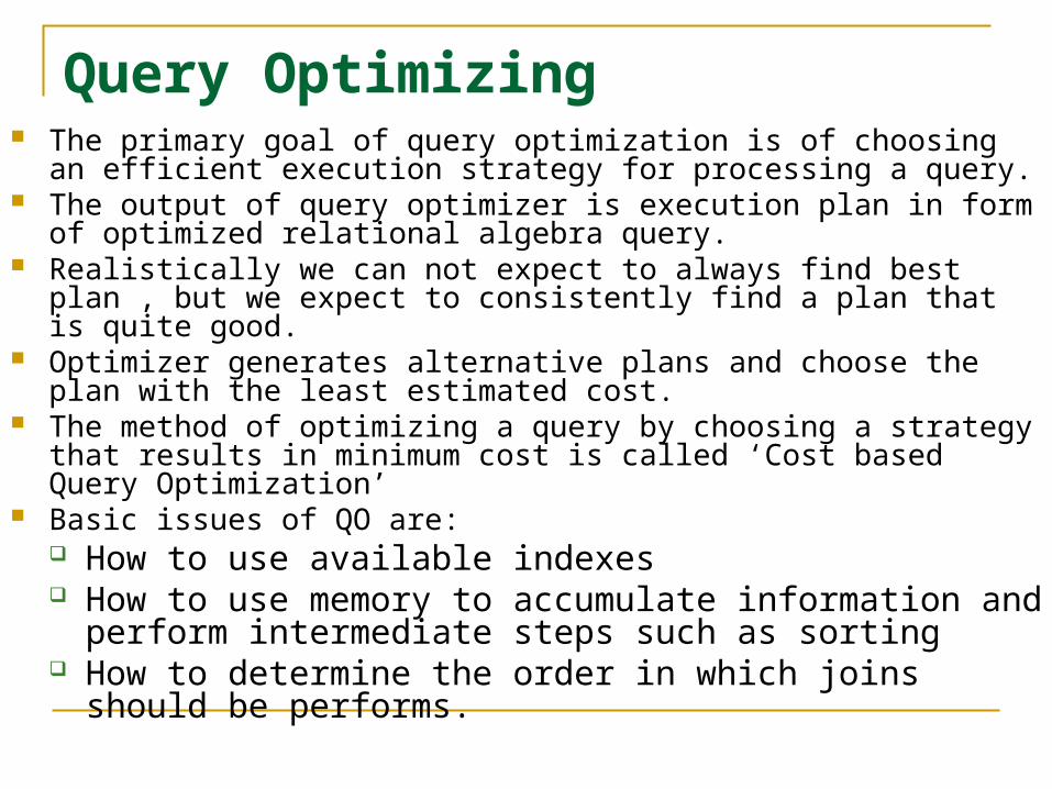
Query Optimizing The primary goal of query optimization is of choosing an efficient

execution strategy for processing a query. The output of query optimizer is execution plan in form of optimized

relational algebra query. Realistically we can not expect to always find best plan , but we expect

to consistently find a plan that is quite good. Optimizer generates alternative plans and choose the plan with the least

estimated cost. The method of optimizing a query by choosing a strategy that results in

minimum cost is called ‘Cost based Query Optimization’ Basic issues of QO are:

How to use available indexes How to use memory to accumulate information and perform

intermediate steps such as sorting How to determine the order in which joins should be

performs.

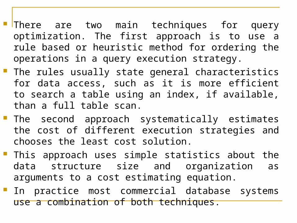
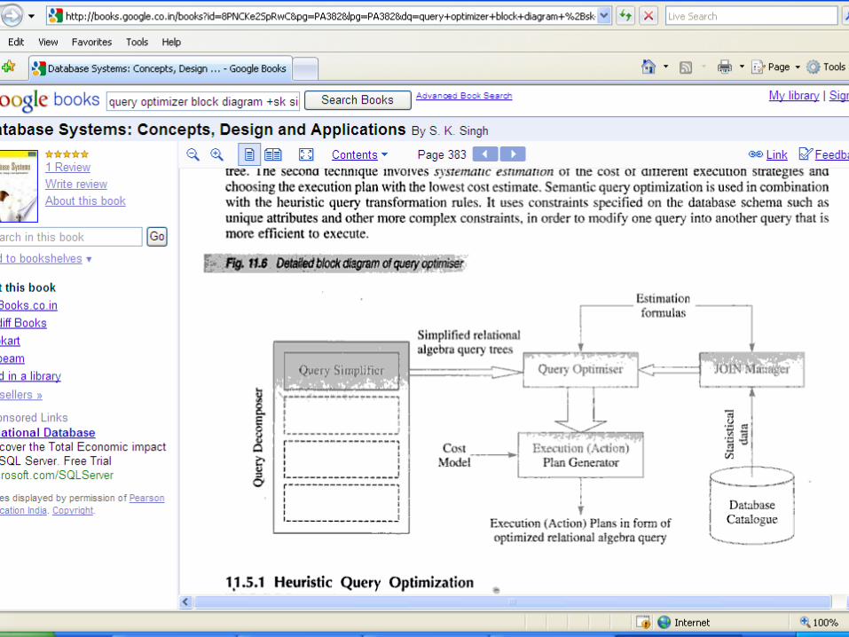
There are two main techniques for query optimization. The first approach is to use a rule based or heuristic method for ordering the operations in a query execution strategy.

The rules usually state general characteristics for data access, such as it is more efficient to search a table using an index, if available, than a full table scan.

The second approach systematically estimates the cost of different execution strategies and chooses the least cost solution.

This approach uses simple statistics about the data structure size and organization as arguments to a cost estimating equation.

In practice most commercial database systems use a combination of both techniques.

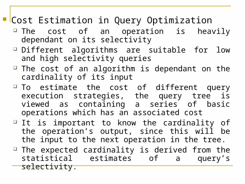
Cost Estimation in Query Optimization The cost of an operation is heavily dependant on its

selectivity Different algorithms are suitable for low and high

selectivity queries The cost of an algorithm is dependant on the cardinality

of its input To estimate the cost of different query execution

strategies, the query tree is viewed as containing a series of basic operations which has an associated cost

It is important to know the cardinality of the operation’s output, since this will be the input to the next operation in the tree.

The expected cardinality is derived from the statistical estimates of a query’s selectivity.

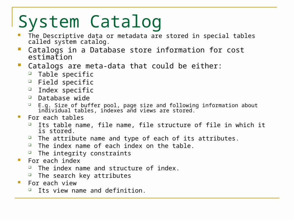
System Catalog The Descriptive data or metadata are stored in special tables called system catalog. Catalogs in a Database store information for cost estimation Catalogs are meta-data that could be either:

Table specific Field specific Index specific Database wide E.g. Size of buffer pool, page size and following information about individual tables, indexes

and views are stored. For each tables

Its table name, file name, file structure of file in which it is stored. The attribute name and type of each of its attributes. The index name of each index on the table. The integrity constraints

For each index The index name and structure of index. The search key attributes

For each view Its view name and definition.

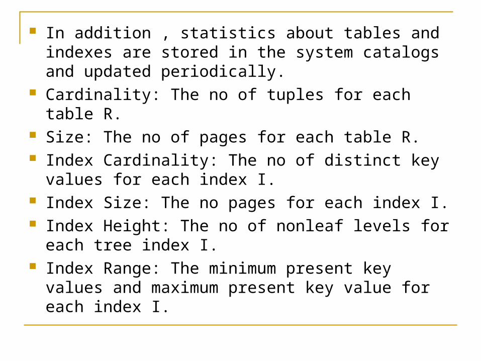
In addition , statistics about tables and indexes are stored in the system catalogs and updated periodically.

Cardinality: The no of tuples for each table R. Size: The no of pages for each table R. Index Cardinality: The no of distinct key values for

each index I. Index Size: The no pages for each index I. Index Height: The no of nonleaf levels for each tree

index I. Index Range: The minimum present key values and

maximum present key value for each index I.

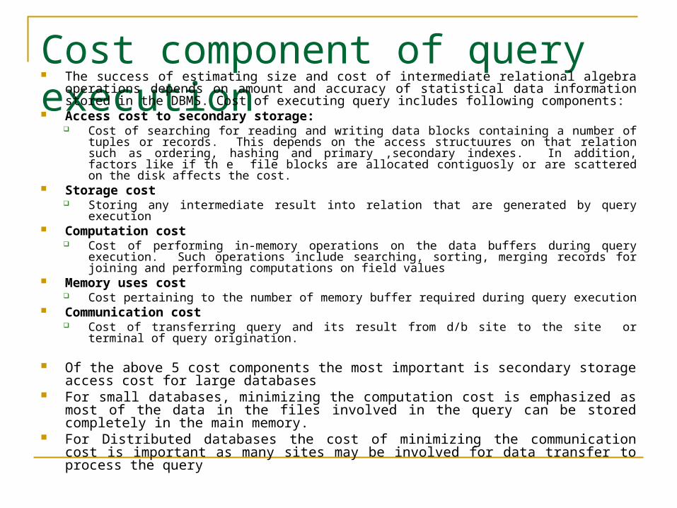
Cost component of query execution The success of estimating size and cost of intermediate relational algebra operations depends on

amount and accuracy of statistical data information stored in the DBMS. Cost of executing query includes following components:

Access cost to secondary storage: Cost of searching for reading and writing data blocks containing a number of tuples or records. This

depends on the access structuures on that relation such as ordering, hashing and primary ,secondary indexes. In addition, factors like if th e file blocks are allocated contiguosly or are scattered on the disk affects the cost.

Storage cost Storing any intermediate result into relation that are generated by query execution

Computation cost Cost of performing in-memory operations on the data buffers during query execution. Such

operations include searching, sorting, merging records for joining and performing computations on field values

Memory uses cost Cost pertaining to the number of memory buffer required during query execution

Communication cost Cost of transferring query and its result from d/b site to the site or terminal of query origination.

Of the above 5 cost components the most important is secondary storage access cost for large databases

For small databases, minimizing the computation cost is emphasized as most of the data in the files involved in the query can be stored completely in the main memory.

For Distributed databases the cost of minimizing the communication cost is important as many sites may be involved for data transfer to process the query

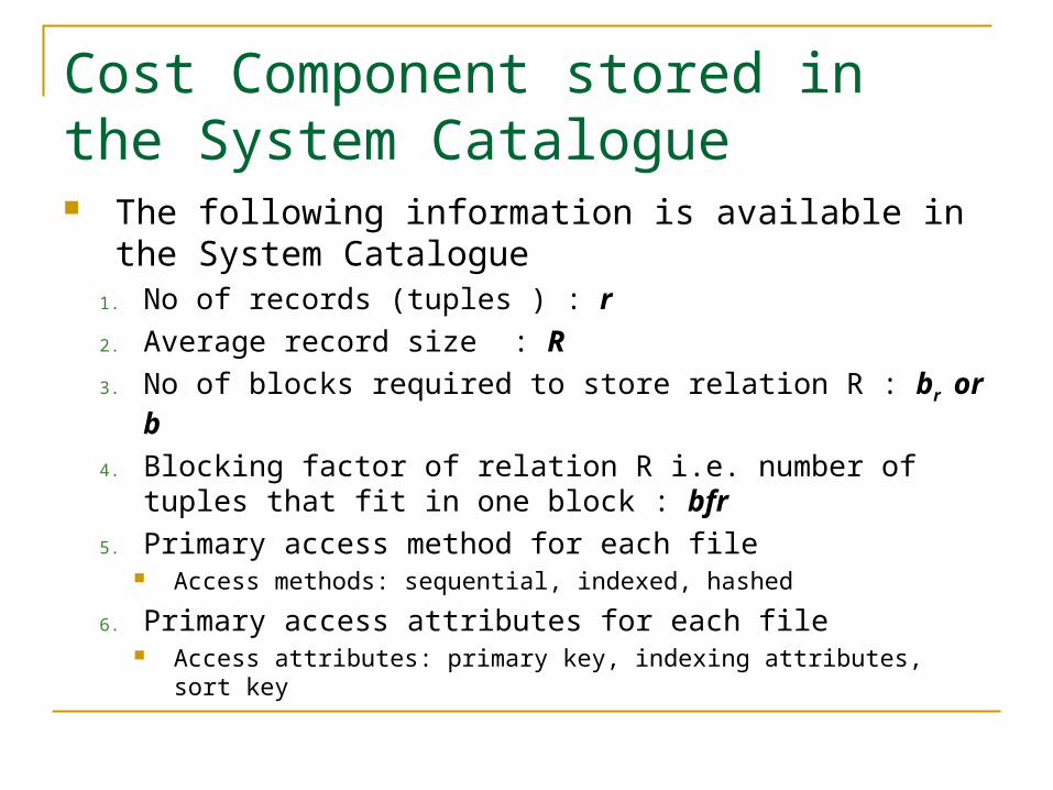
Cost Component stored in the System Catalogue The following information is available in the System

Catalogue1. No of records (tuples ) : r

2. Average record size : R

3. No of blocks required to store relation R : br or b

4. Blocking factor of relation R i.e. number of tuples that fit in one block : bfr

5. Primary access method for each file Access methods: sequential, indexed, hashed

6. Primary access attributes for each file Access attributes: primary key, indexing attributes, sort key

Cost Component stored in the System Catalogue

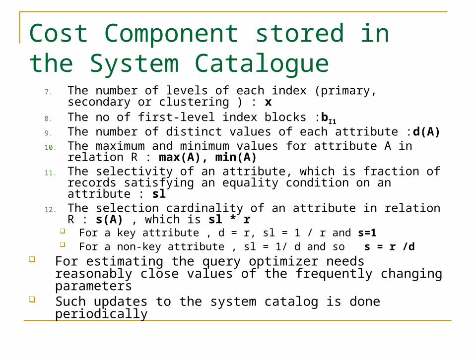
7. The number of levels of each index (primary, secondary or clustering ) : x

8. The no of first-level index blocks :bI1

9. The number of distinct values of each attribute :d(A)10. The maximum and minimum values for attribute A in relation R :

max(A), min(A)11. The selectivity of an attribute, which is fraction of records

satisfying an equality condition on an attribute : sl12. The selection cardinality of an attribute in relation R : s(A) ,

which is sl * r For a key attribute , d = r, sl = 1 / r and s=1 For a non-key attribute , sl = 1/ d and so s = r /d

For estimating the query optimizer needs reasonably close values of the frequently changing parameters

Such updates to the system catalog is done periodically

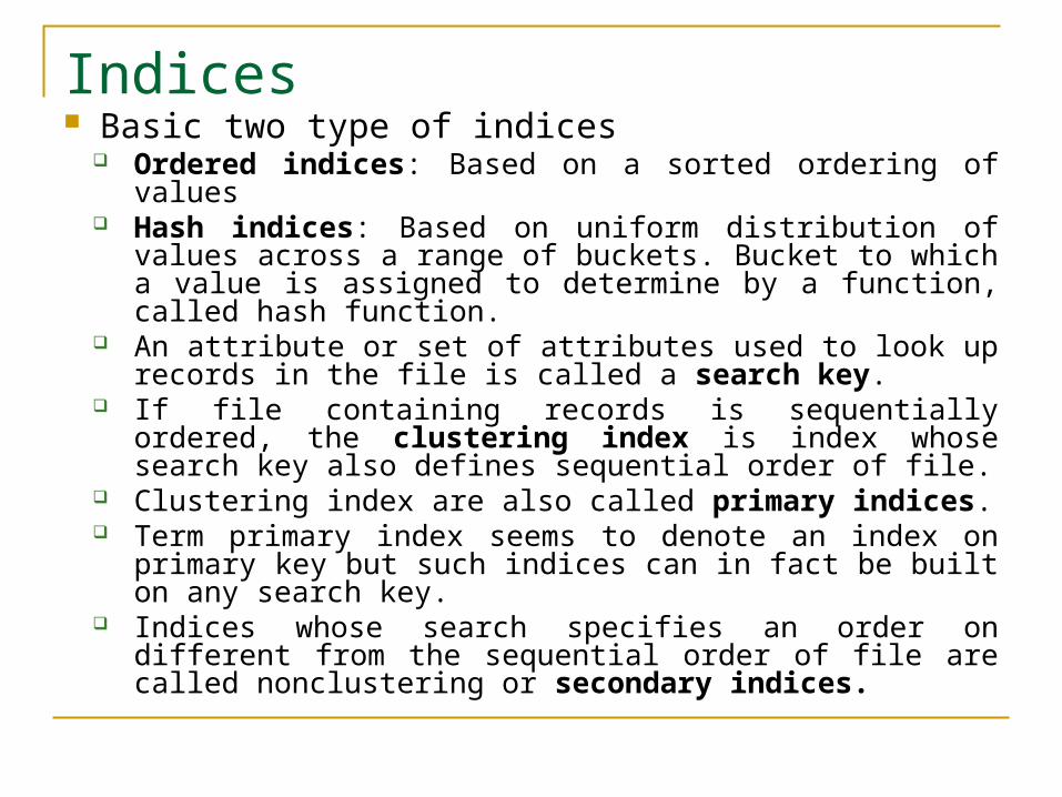
Indices Basic two type of indices

Ordered indices: Based on a sorted ordering of values Hash indices: Based on uniform distribution of values

across a range of buckets. Bucket to which a value is assigned to determine by a function, called hash function.

An attribute or set of attributes used to look up records in the file is called a search key.

If file containing records is sequentially ordered, the clustering index is index whose search key also defines sequential order of file.

Clustering index are also called primary indices. Term primary index seems to denote an index on primary

key but such indices can in fact be built on any search key. Indices whose search specifies an order on different from

the sequential order of file are called nonclustering or secondary indices.

How to measure query cost

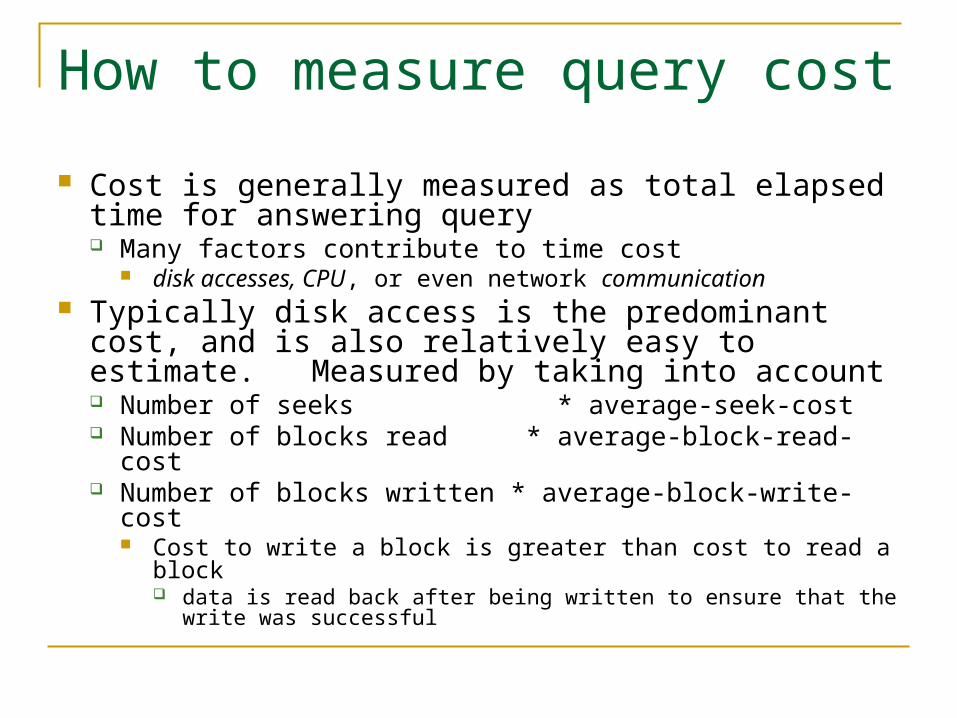
Cost is generally measured as total elapsed time for answering query Many factors contribute to time cost

disk accesses, CPU, or even network communication Typically disk access is the predominant cost, and is

also relatively easy to estimate. Measured by taking into account Number of seeks * average-seek-cost Number of blocks read * average-block-read-cost Number of blocks written * average-block-write-cost

Cost to write a block is greater than cost to read a block data is read back after being written to ensure that the write was

successful

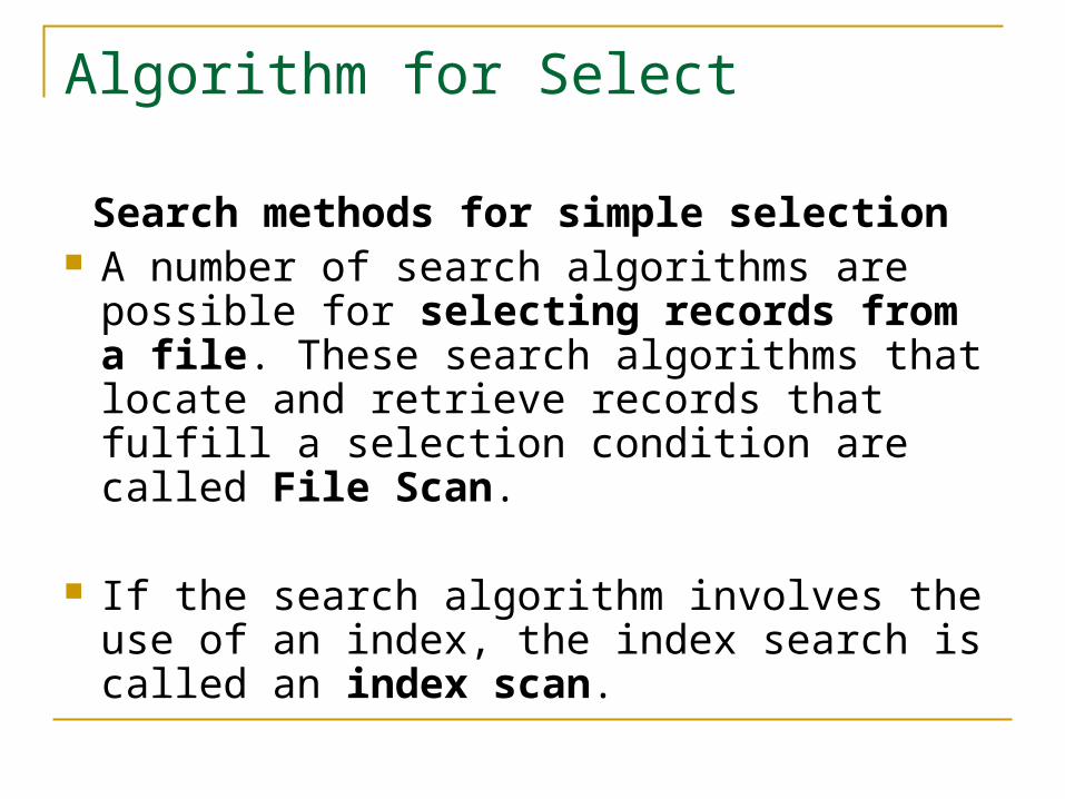
Algorithm for Select

Search methods for simple selection A number of search algorithms are possible

for selecting records from a file. These search algorithms that locate and retrieve records that fulfill a selection condition are called File Scan.

If the search algorithm involves the use of an index, the index search is called an index scan.

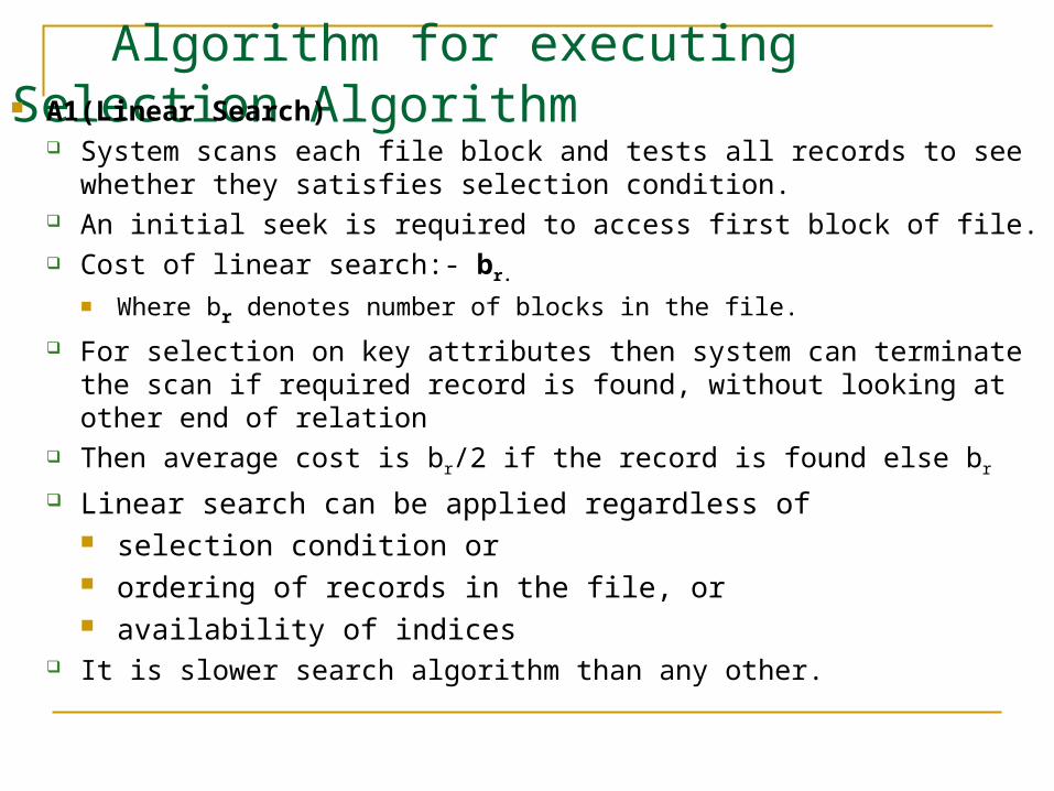
Algorithm for executing Selection Algorithm A1(Linear Search)

System scans each file block and tests all records to see whether they satisfies selection condition.

An initial seek is required to access first block of file. Cost of linear search:- br.

Where br denotes number of blocks in the file.

For selection on key attributes then system can terminate the scan if required record is found, without looking at other end of relation

Then average cost is br/2 if the record is found else br

Linear search can be applied regardless of selection condition or ordering of records in the file, or availability of indices

It is slower search algorithm than any other.

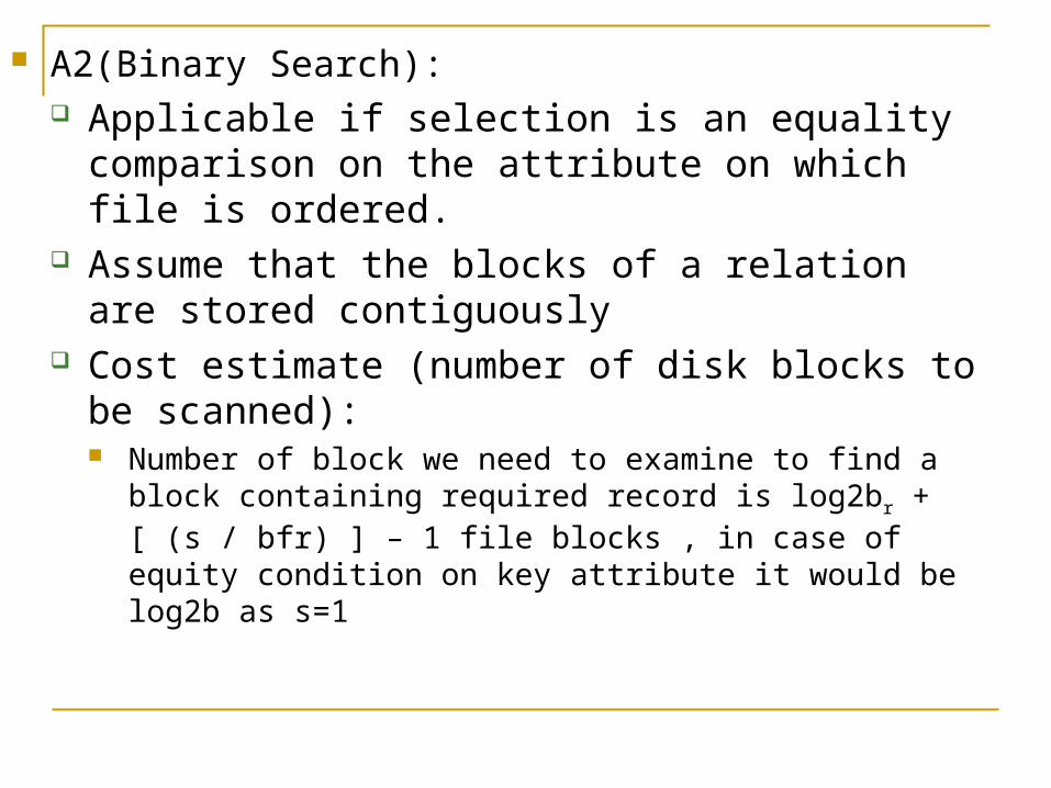
A2(Binary Search): Applicable if selection is an equality comparison on

the attribute on which file is ordered. Assume that the blocks of a relation are stored

contiguously Cost estimate (number of disk blocks to be scanned):

Number of block we need to examine to find a block containing required record is log2br + [ (s / bfr) ] – 1 file blocks , in case of equity condition on key attribute it would be log2b as s=1

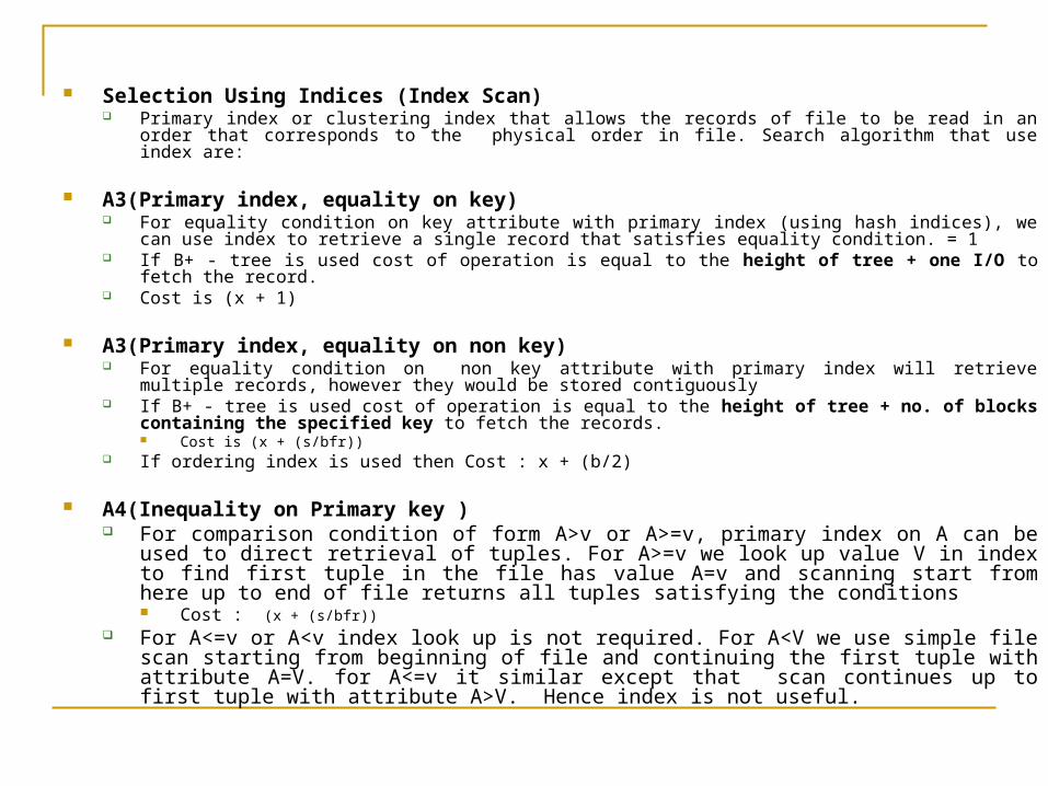
Selection Using Indices (Index Scan) Primary index or clustering index that allows the records of file to be read in an order that corresponds to the

physical order in file. Search algorithm that use index are:

A3(Primary index, equality on key) For equality condition on key attribute with primary index (using hash indices), we can use index to retrieve a single

record that satisfies equality condition. = 1 If B+ - tree is used cost of operation is equal to the height of tree + one I/O to fetch the record. Cost is (x + 1)

A3(Primary index, equality on non key) For equality condition on non key attribute with primary index will retrieve multiple records, however they would be

stored contiguously If B+ - tree is used cost of operation is equal to the height of tree + no. of blocks containing the specified key to

fetch the records. Cost is (x + (s/bfr))

If ordering index is used then Cost : x + (b/2)

A4(Inequality on Primary key ) For comparison condition of form A>v or A>=v, primary index on A can be used to direct retrieval

of tuples. For A>=v we look up value V in index to find first tuple in the file has value A=v and scanning start from here up to end of file returns all tuples satisfying the conditions Cost : (x + (s/bfr))

For A<=v or A<v index look up is not required. For A<V we use simple file scan starting from beginning of file and continuing the first tuple with attribute A=V. for A<=v it similar except that scan continues up to first tuple with attribute A>V. Hence index is not useful.

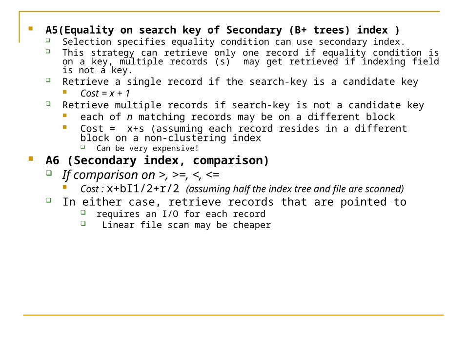
A5(Equality on search key of Secondary (B+ trees) index ) Selection specifies equality condition can use secondary index. This strategy can retrieve only one record if equality condition is on a key, multiple records

(s) may get retrieved if indexing field is not a key. Retrieve a single record if the search-key is a candidate key

Cost = x + 1 Retrieve multiple records if search-key is not a candidate key

each of n matching records may be on a different block Cost = x+s (assuming each record resides in a different block on a non-clustering

index Can be very expensive!

A6 (Secondary index, comparison) If comparison on >, >=, <, <=

Cost : x+bI1/2+r/2 (assuming half the index tree and file are scanned) In either case, retrieve records that are pointed to

requires an I/O for each record Linear file scan may be cheaper

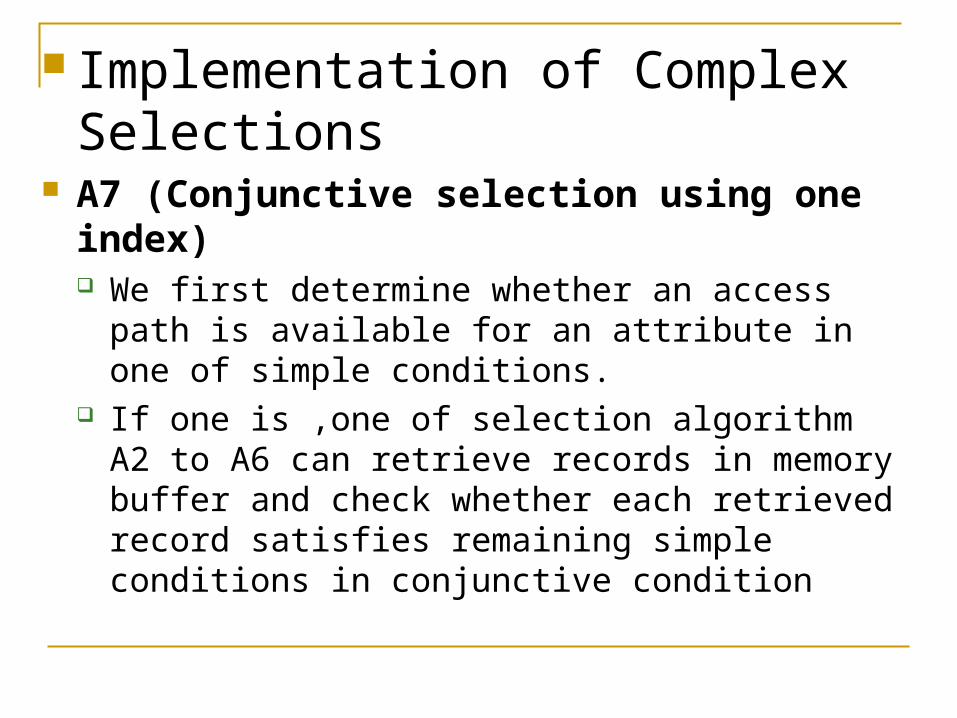
Implementation of Complex Selections

A7 (Conjunctive selection using one index) We first determine whether an access path is

available for an attribute in one of simple conditions.

If one is ,one of selection algorithm A2 to A6 can retrieve records in memory buffer and check whether each retrieved record satisfies remaining simple conditions in conjunctive condition

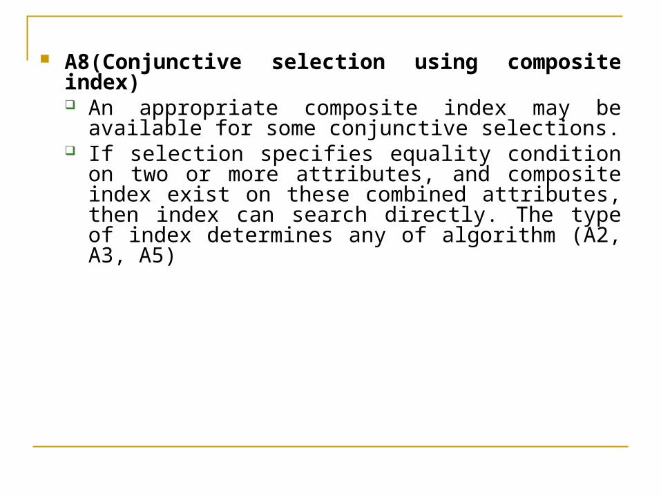
A8(Conjunctive selection using composite index) An appropriate composite index may be available for

some conjunctive selections. If selection specifies equality condition on two or more

attributes, and composite index exist on these combined attributes, then index can search directly. The type of index determines any of algorithm (A2, A3, A5)

Sorting We may build an index on the relation, and then use

the index to read the relation in sorted order. May lead to one disk block access for each tuple which is expensive. It would be more desirable to order the records physically.

For relations that fit in memory, techniques like quick sort can be used.

For relations that don’t fit in memory is called external sorting. The most commonly used method is external sort-merge .

Joins can be implemented more efficiently if input relations are first sorted

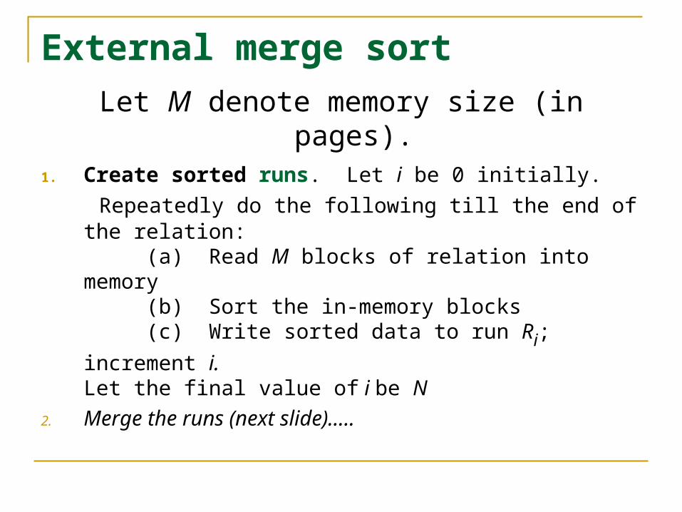
External merge sortLet M denote memory size (in pages).

1. Create sorted runs. Let i be 0 initially. Repeatedly do the following till the end of the relation: (a) Read M blocks of relation into memory (b) Sort the in-memory blocks (c) Write sorted data to run Ri; increment i.

Let the final value of i be N

2. Merge the runs (next slide)…..

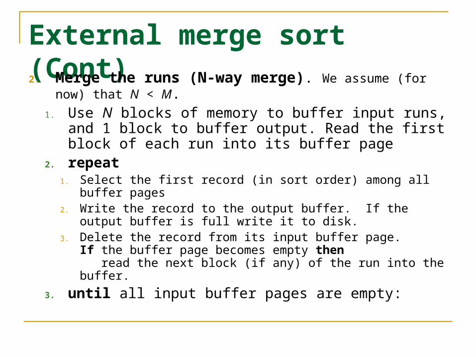
External merge sort (Cont)2. Merge the runs (N-way merge). We assume (for now)

that N < M. 1. Use N blocks of memory to buffer input runs, and 1

block to buffer output. Read the first block of each run into its buffer page

2. repeat1. Select the first record (in sort order) among all buffer pages2. Write the record to the output buffer. If the output buffer is full

write it to disk.3. Delete the record from its input buffer page.

If the buffer page becomes empty then read the next block (if any) of the run into the buffer.

3. until all input buffer pages are empty:

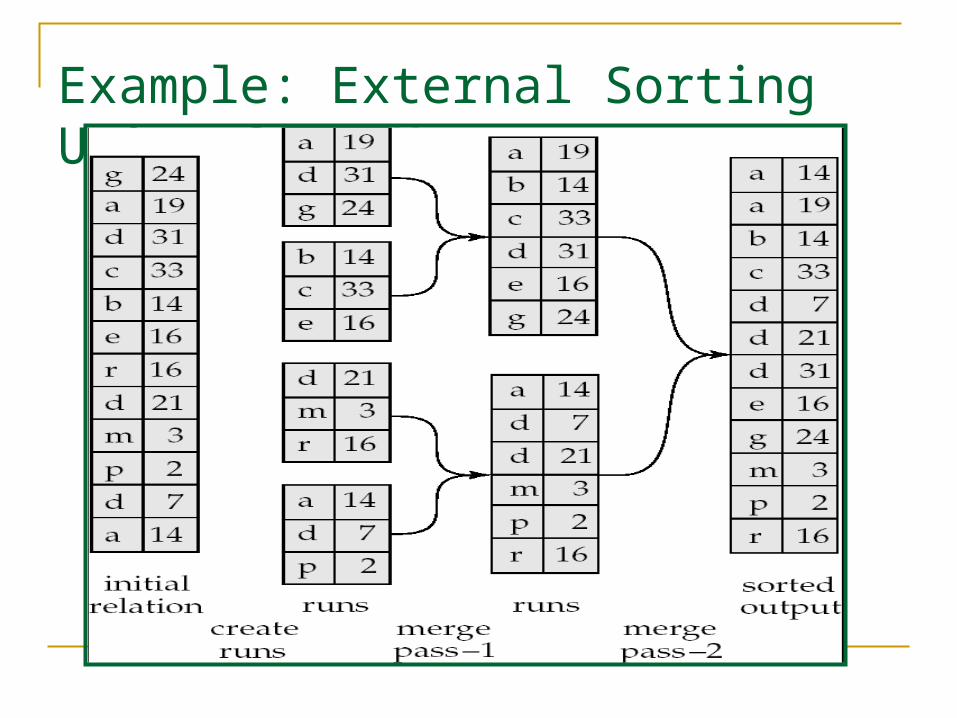
Example: External Sorting Using Sort-Merge

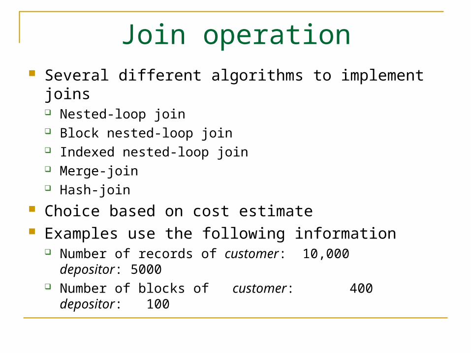
Join operation Several different algorithms to implement joins

Nested-loop join Block nested-loop join Indexed nested-loop join Merge-join Hash-join

Choice based on cost estimate Examples use the following information

Number of records of customer: 10,000 depositor: 5000 Number of blocks of customer: 400 depositor: 100

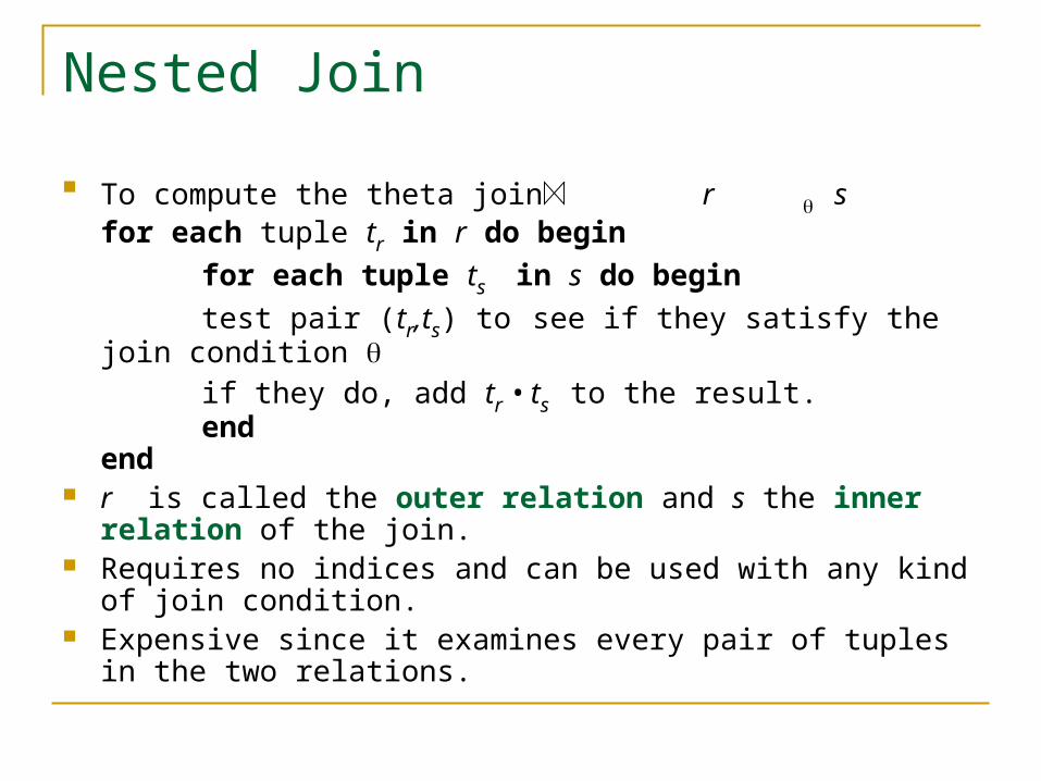
Nested Join

To compute the theta join r sfor each tuple tr in r do begin

for each tuple ts in s do begin

test pair (tr,ts) to see if they satisfy the join condition

if they do, add tr • ts to the result.end

end r is called the outer relation and s the inner relation of the join. Requires no indices and can be used with any kind of join

condition. Expensive since it examines every pair of tuples in the two

relations.

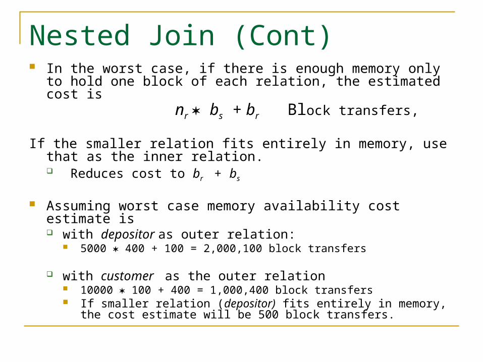
Nested Join (Cont) In the worst case, if there is enough memory only to hold one

block of each relation, the estimated cost is nr bs + br Block transfers,

If the smaller relation fits entirely in memory, use that as the inner relation. Reduces cost to br + bs

Assuming worst case memory availability cost estimate is with depositor as outer relation:

5000 400 + 100 = 2,000,100 block transfers

with customer as the outer relation 10000 100 + 400 = 1,000,400 block transfers If smaller relation (depositor) fits entirely in memory, the cost

estimate will be 500 block transfers.

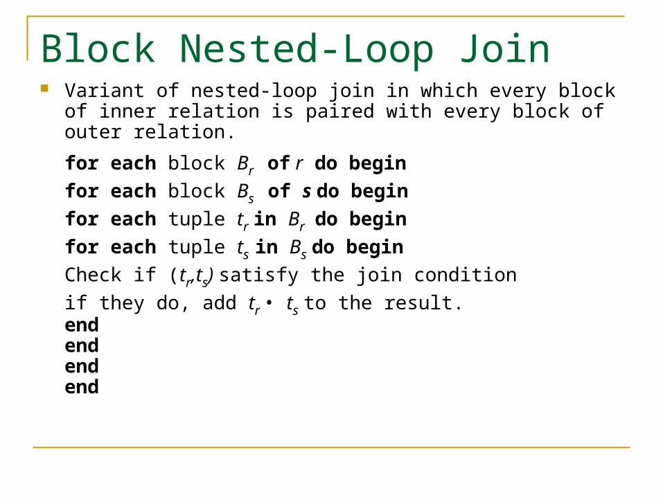
Block Nested-Loop Join Variant of nested-loop join in which every block of inner relation

is paired with every block of outer relation.

for each block Br of r do begin

for each block Bs of s do begin

for each tuple tr in Br do begin

for each tuple ts in Bs do begin

Check if (tr,ts) satisfy the join condition

if they do, add tr • ts to the result.

endend

endend

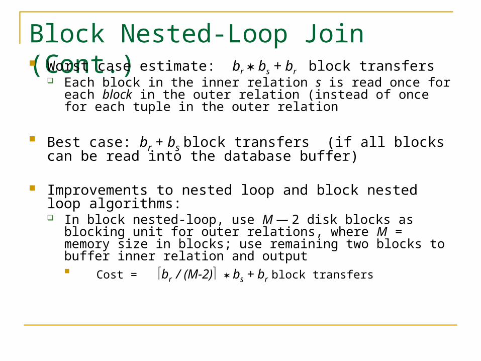
Block Nested-Loop Join (Cont.) Worst case estimate: br bs + br block transfers

Each block in the inner relation s is read once for each block in the outer relation (instead of once for each tuple in the outer relation

Best case: br + bs block transfers (if all blocks can be read into the database buffer)

Improvements to nested loop and block nested loop algorithms: In block nested-loop, use M — 2 disk blocks as blocking unit for

outer relations, where M = memory size in blocks; use remaining two blocks to buffer inner relation and output Cost = br / (M-2) bs + br block transfers

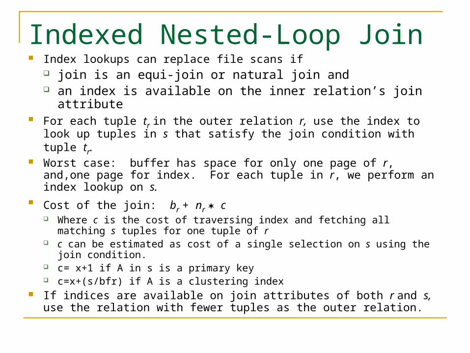
Indexed Nested-Loop Join Index lookups can replace file scans if

join is an equi-join or natural join and an index is available on the inner relation’s join attribute

For each tuple tr in the outer relation r, use the index to look up tuples in s that satisfy the join condition with tuple tr.

Worst case: buffer has space for only one page of r, and,one page for index. For each tuple in r, we perform an index lookup on s.

Cost of the join: br + nr c Where c is the cost of traversing index and fetching all matching s tuples

for one tuple of r c can be estimated as cost of a single selection on s using the join

condition. c= x+1 if A in s is a primary key c=x+(s/bfr) if A is a clustering index

If indices are available on join attributes of both r and s,use the relation with fewer tuples as the outer relation.

Merge Join / Sort Merge Join Used with natural and equi joins The basic idea is to sort both the relations

using sort algorithm on the join attribute and then look for qualifying attributes by essentially merging the two relations

Cost of sorting R : br * log2br

Cost of sorting S : bs * log2bs Cost of Merge : br + bs

Hash Join The hash join algorithm like sort merge

algorithm, can be used for natural joins and equi joins

Identifies partitions in R and S in the partitioning phase and in the probing phase compares tuples in partition R with tuple in partition S for testing equality join conditions

2. Cost:1. Partition Phase Scan R and S once and write once so 2(br + bs)

2. In probing phase we scan each partition once so br +bs

3. Therefore 3(br + bs) when partition fits in memory

Using Heuristics in Query Optimization (17)Query Execution Plans An execution plan for a relational algebra query consists of

a combination of the relational algebra query tree and information about the access methods to be used for each relation as well as the methods to be used in computing the relational operators stored in the tree.

Materialized evaluation: the result of an operation is stored as a temporary relation.

Pipelined evaluation: as the result of an operator is produced, it is forwarded to the next operator in sequence.

Advantages of Pipelining Saves cost of creating temporary relations and reading the result back again

Disadvantages The inputs to the operation are not available all at once for processing, so

choice of algorithms can be restricted

Pipelining In materialization, the output of one operation is

stored in a temporary relation for processing by the next operation.

An alternative approach is to pipeline the results of one operation to another operation without creating a temporary relation to hold the intermediate result.

By using it, we can save on the cost of creating temporary relations and reading the results back in again.

When input table to a unary operator is pipelined into it, we sometimes say that operator are applied on-the-fly

Structure of Query Execution Plans Left Deep Trees

A relational algebra tree where the right-hand relation is always a base relation.

Starts from a relation and constructs result by successively adding an operation till query is completed

Inner relations are always base relations Particularly convenient for pipelined evaluation Advantages: reducing the search space for the optimum strategy

and allowing the query optimizer to be based on dynamic processing techniques.

Disadvantages : In reducing the search space, many alternative execution strategies may not be considered.

Structure of Query Execution Plans Right Deep Trees

A relational algebra tree where the left-hand relation is always a base relation.

Outer relations are base relations. Good for applications with large memory

Starts from a relation and constructs result by successively adding an operation till query is completed

Linear Tree Combination of Left and Right Deep trees

One side is always a relation

Bushy (non-linear trees) Both inputs to a binary operation can be intermediate result

Advantages : Is flexible