queueing basics - denninginstitute.com

Queueing Basics

P. J. DenningFor CS471/571

© 2002, P. J. Denning

© 2002, P. J. Denning 2

Performance Questions

• Performance questions always part of asystems discussion– throughput (jobs per second)– response time (seconds)– congestion and bottlenecks– capacity planning

• How to measure and forecast?

© 2002, P. J. Denning 3

Airline Reservations Example

• 1000 reservation agents around the USA.• “Disk farm” in New York City.• Each agent issues new transactions against

the database every 60 seconds.• Every transaction accesses the directory disk

an average of 10 times.• The directory disk takes an average of 5

milliseconds to serve a request and is in use80% of the time.

© 2002, P. J. Denning 4

• What is the throughput (jobs per second)completed by the entire system?

• What is the response time experienced by anagent waiting for a transaction?

• Can these questions be answered precisely?Approximately? Not at all?

© 2002, P. J. Denning 5

Tools• Queueing theory gives the basic tools for answering

such questions.• The theory deals with randomness in physical

processes such as– the arrival times of agent requests– the service times at the disks and CPUs– lengths of queues– variations in response times

• The theory allows us to characterize the performancemeasures statistically, in terms of averages, given thestatistics of arrivals and services

© 2002, P. J. Denning 6

Erlang’s Model

• The first use of queueing theory inengineering occurred around 1909 when theDanish engineer A. K. Erlang modeledtelephone systems, including interarrivaltimes and lengths of calls.

• His model gave accurate predictions of thenumber of active calls, important for thesizing of telephone switching centers.

© 2002, P. J. Denning 7

telephoneswitching

center

Set of usersinitiating calls

at random times

Set of users receiving calls and hanging up at random times

User i picks up the phone;gets a dial tone;dials the number of user j;who picks up the phone;they talk together;and they hang up.

Assumptions: The next call starts randomly in time with rate a. A call terminates randomly in time with rate b. State of system is n, number of calls in progress. Number of switch points, N, is less than number of users.

Question: What is the probability P(n) that the system will be the state where n calls are simultaneously in progress?

Rationale: P(N) is probably that all N crosspoints will be in use. No dial tone if someone attempts a call when state n > N.

© 2002, P. J. Denning 8

What does "random rate a" mean?

timedt

probability of an event in this tiny time interval (dt)is a•dt independent of every other disjoint time interval

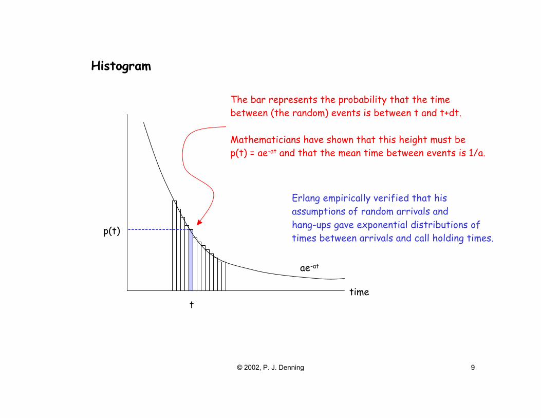
With this assumption, the histogram of times between eventsis exponential with parameter a and mean 1/a. (Interpretationon next picture.)

© 2002, P. J. Denning 9

time

ae-at

t

p(t)

The bar represents the probability that the timebetween (the random) events is between t and t+dt.

Mathematicians have shown that this height must bep(t) = ae-at and that the mean time between events is 1/a.

Histogram

Erlang empirically verified that hisassumptions of random arrivals and hang-ups gave exponential distributions oftimes between arrivals and call holding times.

© 2002, P. J. Denning 10

0 1 2 n-1 n

Erlang's state space

a a a a a a

bbbbbb

Up-transitions occur with each new call, at rate a.Down transitions occur with each hangup, at rate b.Assume a<b so that system is not overwhelmed.The rates are independent of state.There is no limit on the maximum number of calls.Let p(n) denote the fraction of time system state = n.

At any cut, the flow up must balancethe flow down, or p(n-1)a = p(n)bthus p(n) = (a/b)p(n-1) = (a/b)n p(0)which is a geometric series. The sumof the series for all p(n) must be 1: S p(n) = p(0) S (a/b)n = p(0)/(1-(a/b))or p(0) = 1-(a/b)

© 2002, P. J. Denning 11

It is usually easier to compute the p(n) through simple iterative methodsthan to evaluate a closed-form mathematical expression, especially whenthe mathematics allow n to become infinite whereas n is bounded in thereal system.

Limit the state diagram to states 0,1,...,N. Use this procedure:

(1) Guess p(0) -- e.g., set p(0)=1. (2) Compute p(n) = p(n-1)(a/b) for n=1,...,N. (3) Compute the sum S of the p(n). (S is called the “normalizing constant”) (4) Replace each p(n) with p(n)/S.

Now we have a valid probability distribution: it satisfies the recursionand sums to 1.

When p(N) is small, the error between the math expression and thecomputer evaluation is small.

© 2002, P. J. Denning 12

example (see next page)

new-call requests every 120 sec (a = 1/120)

average call lasts 100 sec(b = 1/100)

What is the median number of active calls?(3)

What is probability that the telephone exchange is saturated?(0.07%)

What is the probability that the telephone exchange is idle?(16%)

What is the 90th percentile of the number of active calls?(11)

© 2002, P. J. Denning 13

raw p(n): "guess" p(0)=1,then compute each newp(n) = (a/b)p(n-1). Getsratios right.

norm p(n): divide eachraw p(n) by the sum ofall p(n). Now they alladd up to 1 and have theproper ratios.

cum p(n): the cumulativesum of p(0)+...+p(n).Shows approach to 1.0as n increases.

inf approx: pretends ngoes to infinity. Startswith p(0) = 1-a/b anduses the same recursion.

© 2002, P. J. Denning 14

Servers

• Server is a station that satisfies certain taskswithin jobs.

• Has one or more internal parallel processors(we assume one).

• Has a queueing mechanism to make tasks notin service wait.

• Has input point for task arrivals.• Has output point for task completions.

© 2002, P. J. Denning 15

i

i

i

simple notation for single serverwith FIFO queueing

more complex notation for single serverwith FIFO queueing, showing the queue.

notation for multi-server with FIFOqueueing, showing internal processors.

© 2002, P. J. Denning 16

Network of Servers

Set of servers with interconnection pathways.

Open or closed.

Closed network includes all its customers ina finite population of N jobs.

new programs

CPU

I/O

I/O

I/O

© 2002, P. J. Denning 17

Measuring a Server

server

Aarrivals

Ccompletions

busy time, B

observation period: T

arrival rate: l = A/T

completion rate: X = C/T

utilization: U = B/T

mean service time: S = B/C

© 2002, P. J. Denning 18

Measuring a Server

server

Aarrivals

Ccompletions

busy time, B

Flow balance: A=C

Utilization law: U = SXUtilization law: U = SX

© 2002, P. J. Denning 19

Measuring a Server

serverX

load n(t)

Mean load: Q = W/T

Mean response time: R = W/C

jobs

time, t0 T

n(t)

Little’s Law: Q = RXLittle’s Law: Q = RX

areaW

© 2002, P. J. Denning 20

Measuring a Network

new programs

CPU

I/O

I/O

I/OX1

X2

X3

X4

X

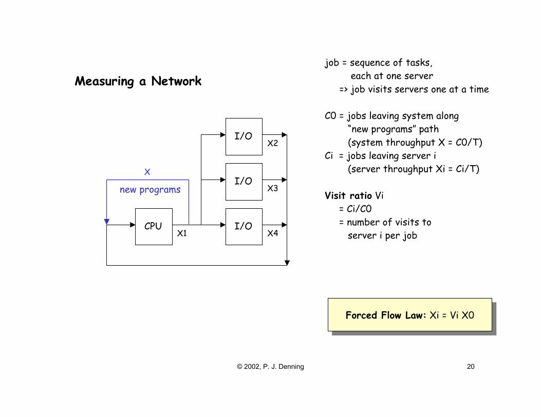
job = sequence of tasks, each at one server => job visits servers one at a time

C0 = jobs leaving system along “new programs” path (system throughput X = C0/T)Ci = jobs leaving server i (server throughput Xi = Ci/T)

Visit ratio Vi = Ci/C0 = number of visits to server i per job

Forced Flow Law: Xi = Vi X0Forced Flow Law: Xi = Vi X0

© 2002, P. J. Denning 21

new programs

CPU

I/O

I/O

I/OX1

X2

X3

X4

X

Forced Flow Law: Xi = Vi XForced Flow Law: Xi = Vi X

Flow at any one pointin the system determines

flow everywhere

Measuring a Network

© 2002, P. J. Denning 22

Measuring a Network -- Central Server System Example

new programs

CPU

I/O

I/O

I/O

S2,V2

X

parameters of system:

Si = mean service time per visit to server i

Vi = mean number of visits to server i

N = total number of jobs in the system

S3,V3

S4,V4S1,V1

© 2002, P. J. Denning 23

Measuring a Network -- Time Sharing System Example

N, Z

CPU

I/O

I/O

I/O

S2,V2

X

parameters of system:

Si = mean service time per visit to server i

Vi = mean number of visits to server i

N = total number of jobs in the system

Z = mean think time between requests for the system

S3,V3

S4,V4S1,V1

____________

User model: (think, wait)*

Execution model: (CPU)(I/O, CPU)*

User model: (think, wait)*

Execution model: (CPU)(I/O, CPU)*

© 2002, P. J. Denning 24

Measuring a Network -- Time Sharing System Example

N, Z

CPU

I/O

I/O

I/O

S2,V2

X

S3,V3

S4,V4S1,V1

____________

Little’s Law for the entirebox says

N = (R+Z) X

R

Response Time Law:R = N/X - Z

Response Time Law:R = N/X - Z

© 2002, P. J. Denning 25

diskSi,Vi

1000 agentsthink time 60 sec

____________

Airline Reservations System Example

10 accesses per transactionservice time 5 msec per access

utilization 80%

© 2002, P. J. Denning 26

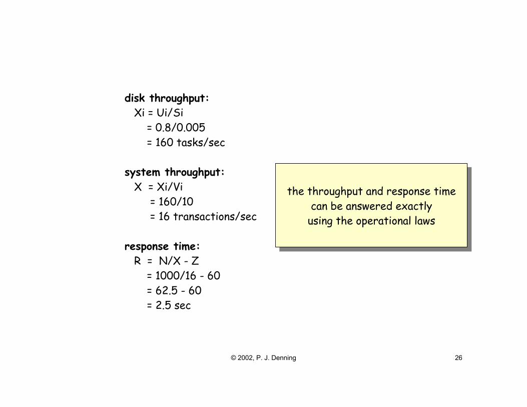
disk throughput: Xi = Ui/Si = 0.8/0.005 = 160 tasks/sec

system throughput: X = Xi/Vi = 160/10 = 16 transactions/sec

response time: R = N/X - Z = 1000/16 - 60 = 62.5 - 60 = 2.5 sec

the throughput and response timecan be answered exactlyusing the operational laws

the throughput and response timecan be answered exactlyusing the operational laws

© 2002, P. J. Denning 27

Prediction in Airline Reservations System Example

What if disk access method were changed to reduceaccesses to 8 per transaction?

Well ...

Xi = 160 accesses per second

X = Xi/Vi = 160/8 = 20 transactions per second

R = 1000/20 - 60 = 50 - 60 = -10 ???

© 2002, P. J. Denning 28

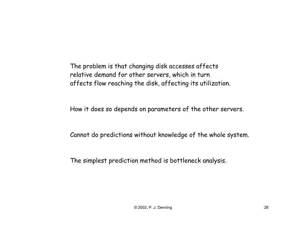
The problem is that changing disk accesses affectsrelative demand for other servers, which in turnaffects flow reaching the disk, affecting its utilization.

How it does so depends on parameters of the other servers.

Cannot do predictions without knowledge of the whole system.

The simplest prediction method is bottleneck analysis.

© 2002, P. J. Denning 29

Bottleneck Analysis• Bottleneck: a choke point in the system’s flow structure -- tasks

pile up there because they flow past too slowly.• Utilization and forced flow laws tell that Ui = XiSi = ViSiX = DiX.

(Define demand Di = ViSi.)• For given X, servers with larger demand Di have higher utilizations;

server with highest demand Di has highest utilization.• Bottleneck server b is one for which Db = max{Di} .• Since utilizations cannot exceed 1, server with highest demand

limits throughput: X = Ub/Db ≤ 1/Db .• This also limits response time: R = N/X - Z ≥ N Db - Z .

© 2002, P. J. Denning 30

N

jobs/sec

1/Db

X(N)

© 2002, P. J. Denning 31

N

secN Db - Z

R(1) = ∑ Di

1 Z/Db

R(N)

© 2002, P. J. Denning 32

Bottleneck Example

N, Z

CPU DISK

X

S2,V2S1,V1

____________

Given: CPU time per job 1 sec 100 disk accesses per job 20 msec per disk access think time 30 sec

What are model parameters? V2 = 100 S2 = 0.02 sec V1 = 1+V2 (why?) = 101 S1 = D1/V1 = 1/101 = 0.0099 sec. D1 = V1S1 = 1 sec. D2 = V2S2 = (100)(0.02) = 2 sec. Z = 30

© 2002, P. J. Denning 33

Bottleneck Example --throughput asymptotes

N

jobs/sec

0.5

X(N)

DISK is the bottleneckb=2 and Db = 2.X ≤ 1/Db = 0.5

© 2002, P. J. Denning 34

Bottleneck Example --response time asymptotes

N

sec2N-30DISK

R(1) = 3

1 15

R(N)

N-30CPU

30

© 2002, P. J. Denning 35

Bottleneck Example

Faster disk has access time 15 msec.Is 5-sec response time feasible with40 users?

Change S2 to 0.015 Now D2 = (100)(0.015) = 1.5 DISK is still bottleneck (D1 = 1.0) R(N) ≥ NDb-Z = (40)(1.5)-30 = 30 sec.

No, 5-sec response time not feasible.

© 2002, P. J. Denning 36

N

sec 2N-30DISK

R(1) = 3

1 15

R(N)

30

(1.5)N-30DISK

20

R(1) = 2.5

40

N-30CPU

© 2002, P. J. Denning 37

Bottleneck Example

New index structure reduces diskaccesses to 50 on the faster disk.Is 5-sec response time feasible with40 users?

Change V2 to 50 Now D2 = (50)(0.015) = 0.75 Now CPU is bottleneck (D1 = 1.0) R(N) ≥ NDb-Z = (40)(1)-30 = 10 sec.

No, 5-sec response time not feasible. Toachieve it, need to speed up the CPU.

© 2002, P. J. Denning 38

Bottleneck Example

Use 2x faster CPU plus the improveddisk. Is 5-sec response time feasiblewith 40 users?

Change D1 to 0.5 sec. Now DISK is bottleneck (D2 = 0.75) R(N) ≥ NDb-Z = (40)(0.75)-30 = 0 sec. Also R(N) ≥ R(1) = D1+D2 = 1+0.75 = 1.75

Yes, 5-sec response time is feasible.

© 2002, P. J. Denning 39

Bottleneck Example

When speeding up a bottleneck,watch our for the next bottleneck.

Response time objective may needseveral servers to become faster so

that all potential bottlenecks are havetheir asymptotes to the right of the desired

operating point.

When speeding up a bottleneck,watch our for the next bottleneck.

Response time objective may needseveral servers to become faster so

that all potential bottlenecks are havetheir asymptotes to the right of the desired

operating point.

© 2002, P. J. Denning 40

Computational Algorithms

• Bottleneck analysis useful to discover ifdesired operating points are in feasibleregions and tell which servers needadditional capacity.

• What algorithm can we use to calculate theentire curve of R(N)?

• The Mean Value Analysis (MVA) algorithmdoes this.

© 2002, P. J. Denning 41

Mean Value Analysis (MVA)

• MVA algorithm calculates several meanvalues together --– Ri = mean response time per visit to server i– R = mean service time per visit to the system– X = throughput of the system– Qi = mean queue length at server i

• MVA does this for n = 0, 1, ... , N.• The set of mean values for n-1 is used to

compute the set of mean values for n.

© 2002, P. J. Denning 42

set all Qi(0) = 0for n = 1 to N do { set all Ri(n) = Si*(1+Qi(n-1)) set R(n) = sum of {Vi*Ri(n)} set X(n) = n/(R(n)+Z) set all Qi(n) = X(n)*Vi*Ri(n) }exit

MVA:

© 2002, P. J. Denning 43


MVA:

Little's Law says that Qi = XiRiForced Flow Law says Xi = XVi

Combining them says Qi = XViRi

© 2002, P. J. Denning 45


MVA:

Response time is the sum ofper-visit server response timesweighted by number of visits to

each server.

© 2002, P. J. Denning 46


MVA:

Per-visit server response time at aserver is the arriver's mean service

plus the mean service needed by everyonequeued in front of the arriver.

The arriver sees the same mean queueas would outside observer in a system with

one less job (arriver removed).

© 2002, P. J. Denning 47

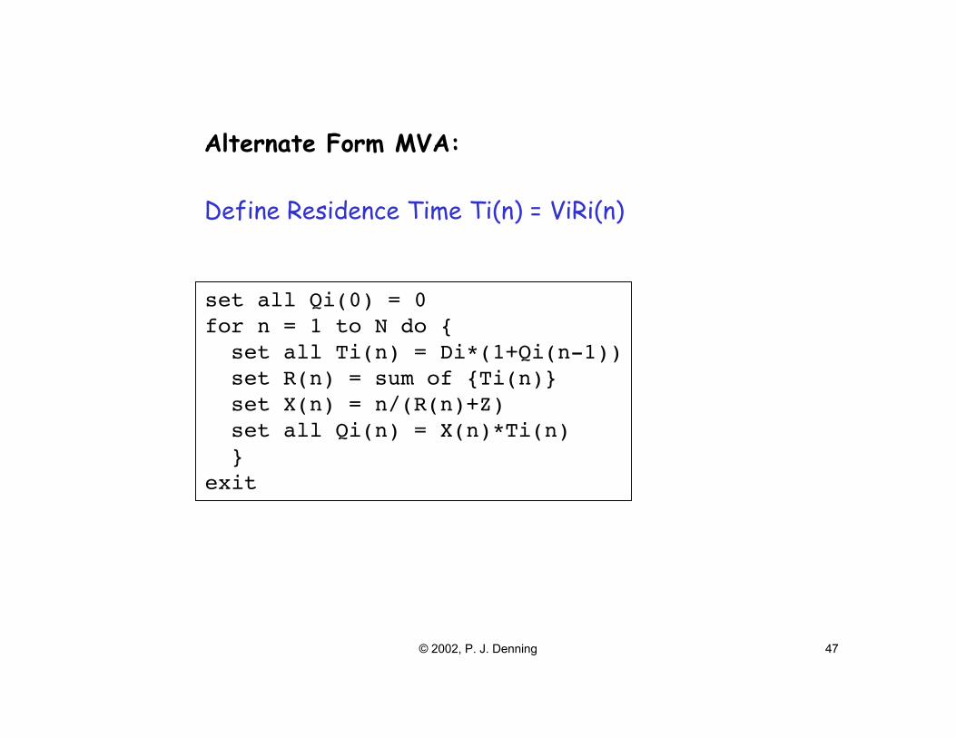
set all Qi(0) = 0for n = 1 to N do { set all Ti(n) = Di*(1+Qi(n-1)) set R(n) = sum of {Ti(n)} set X(n) = n/(R(n)+Z) set all Qi(n) = X(n)*Ti(n) }exit

Alternate Form MVA:

Define Residence Time Ti(n) = ViRi(n)

© 2002, P. J. Denning 48

n

0123...

Q1 ... QKT1 ... TK

K+1 K+2

0 ... 0

1 ... K K+3 ... 2K+2

Having filled in one row, the algorithmfills in values in the next row in the order

indicated by the numbers 1, ..., 2K+2.

When done, the R-column containsthe complete curve R(n).

Same for X-column.

Having filled in one row, the algorithmfills in values in the next row in the order

indicated by the numbers 1, ..., 2K+2.

When done, the R-column containsthe complete curve R(n).

Same for X-column.

R X

© 2002, P. J. Denning 49

Note that X approachesa saturation value,

1/D1 = 0.5

Note that X approachesa saturation value,

1/D1 = 0.5

Note that R approachesa saturation line,n*Db-Z = 2*n-30

Note that R approachesa saturation line,n*Db-Z = 2*n-30

© 2002, P. J. Denning 51

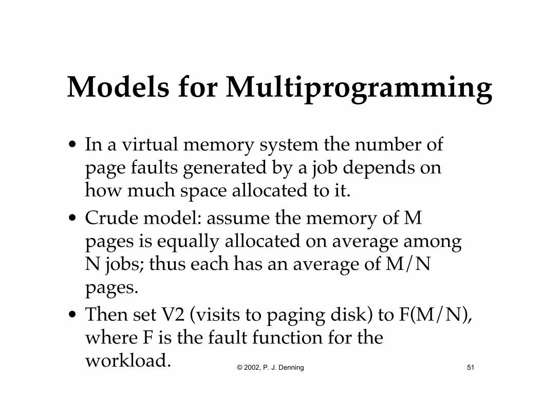
Models for Multiprogramming

• In a virtual memory system the number ofpage faults generated by a job depends onhow much space allocated to it.

• Crude model: assume the memory of Mpages is equally allocated on average amongN jobs; thus each has an average of M/Npages.

• Then set V2 (visits to paging disk) to F(M/N),where F is the fault function for theworkload.

© 2002, P. J. Denning 52

• This means D2 is a function of N.• As N increases, F(M/N) increases (less

space), and D2(N) increases.• The throughput bound is now min{1/D1,

1/D2(N)}.• For small N CPU may be bottleneck and X(N)

≤ 1/D1.• For large N, DISK is the bottleneck and X(N)

≤ 1/D2(N).

© 2002, P. J. Denning 53

N

jobs/sec

1/D1

X(N)

1/D2(N)

Bottlenecks explainthrashing.

Can use the MVA modelto evaluate. To calculate

X(N), set D2=D2(N)and compute X(n) for

n=1,...,N with thatfixed value of D2. Repeat

for each value of N.

(Model assumes that thedemands are constantacross all rows; fails if

this is not so.)

Bottlenecks explainthrashing.

Can use the MVA modelto evaluate. To calculate

X(N), set D2=D2(N)and compute X(n) for

n=1,...,N with thatfixed value of D2. Repeat

for each value of N.

(Model assumes that thedemands are constantacross all rows; fails if

this is not so.)Optimal level ofmultiprogramming occurs

near N that makesD1 = D2(N)

(if bounds cross).

Optimal level ofmultiprogramming occurs

near N that makesD1 = D2(N)

(if bounds cross).

© 2002, P. J. Denning 54

Example output from a model in which D2 isalways larger than D1 and thus the bounds donot cross. However, X(N) still shows a peakand thrashing. (A(N) is an approximation thatdoes not work well.)

queueing basics - denninginstitute.com

Documents