queueing models - university of pittsburghpeople.cs.pitt.edu/~lipschultz/cs1538/08_queueing.pdf ·...
TRANSCRIPT
Queueing Models
CS1538: Introduction to Simulations
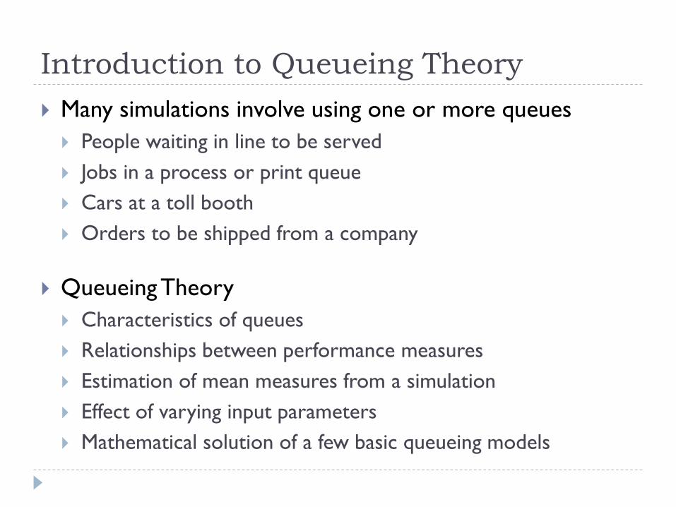
Introduction to Queueing Theory
Many simulations involve using one or more queues
People waiting in line to be served
Jobs in a process or print queue
Cars at a toll booth
Orders to be shipped from a company
Queueing Theory
Characteristics of queues
Relationships between performance measures
Estimation of mean measures from a simulation
Effect of varying input parameters
Mathematical solution of a few basic queueing models
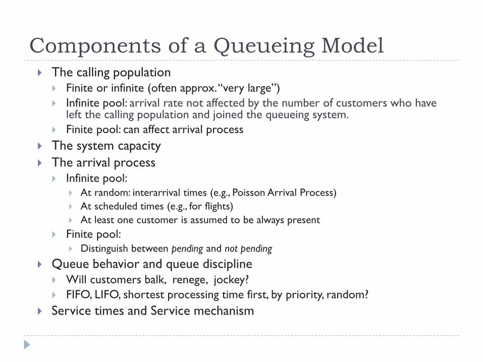
Components of a Queueing Model The calling population
Finite or infinite (often approx. “very large”)
Infinite pool: arrival rate not affected by the number of customers who have left the calling population and joined the queueing system.
Finite pool: can affect arrival process
The system capacity
The arrival process Infinite pool:
At random: interarrival times (e.g., Poisson Arrival Process)
At scheduled times (e.g., for flights)
At least one customer is assumed to be always present
Finite pool:
Distinguish between pending and not pending
Queue behavior and queue discipline Will customers balk, renege, jockey?
FIFO, LIFO, shortest processing time first, by priority, random?
Service times and Service mechanism
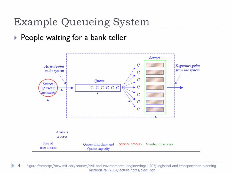
Example Queueing System
4
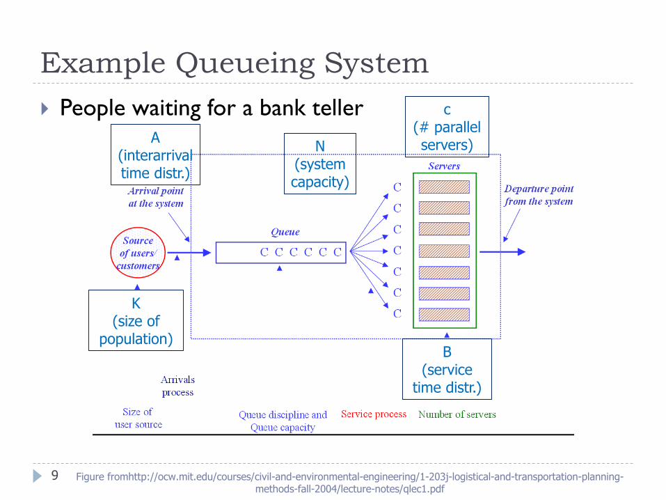
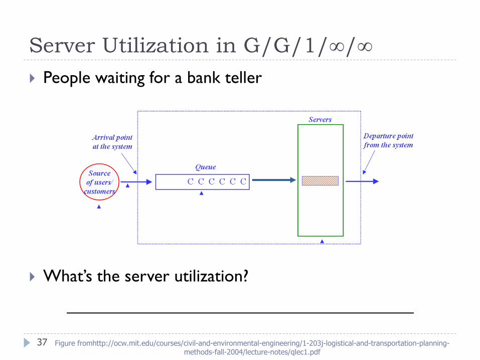
People waiting for a bank teller
Figure fromhttp://ocw.mit.edu/courses/civil-and-environmental-engineering/1-203j-logistical-and-transportation-planning-methods-fall-2004/lecture-notes/qlec1.pdf
Applications of Queueing Theory
Familiar Queues:
Check-ins at airports or hotels
ATMs
Fast food restaurants
Phone center lines (and telephone exchanges…)
Toll booths
Busy street intersections
Spatially-distributed services (e.g. police, fire)
Economic Analyses
Tradeoff between customer satisfaction & system utilization
5
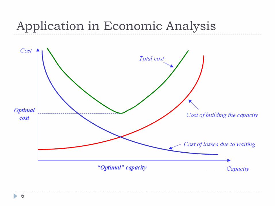
Application in Economic Analysis
6
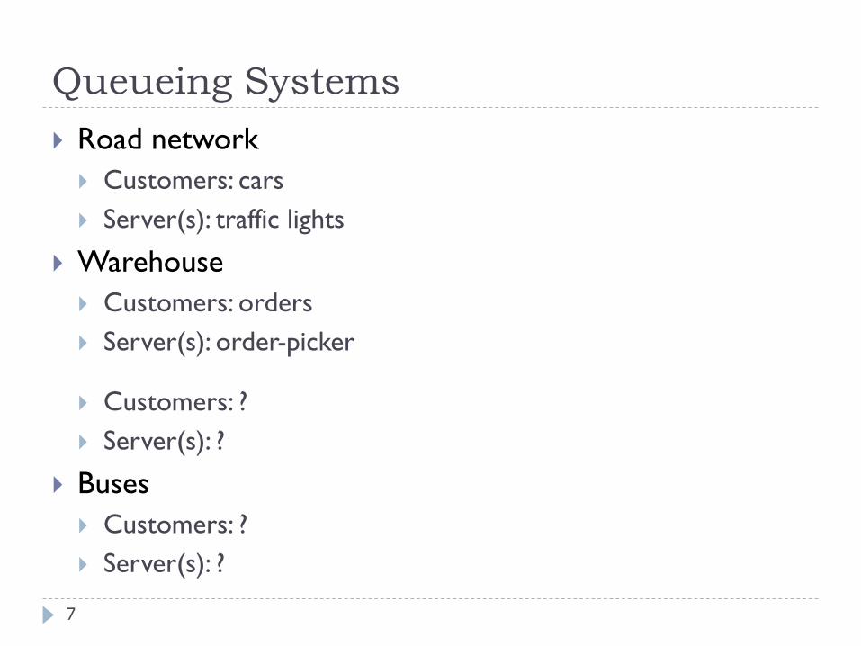
Queueing Systems
Road network
Customers: cars
Server(s): traffic lights
Warehouse
Customers: orders
Server(s): order-picker
Customers: ?
Server(s): ?
Buses
Customers: ?
Server(s): ?
7
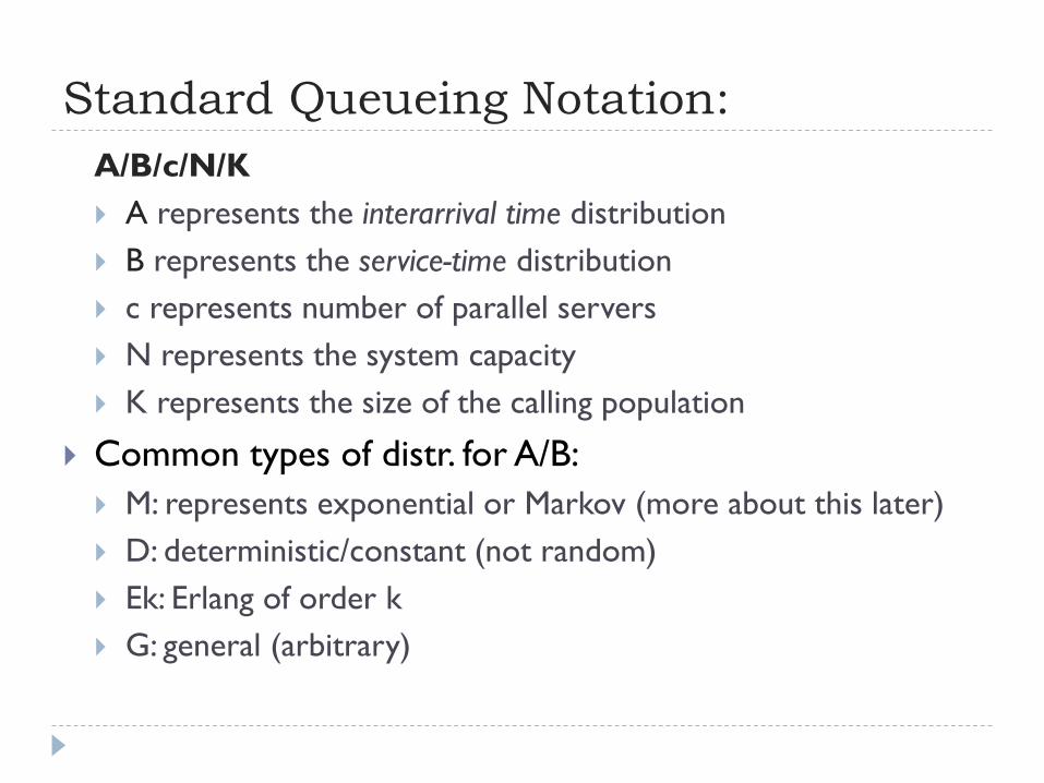
Standard Queueing Notation:
A/B/c/N/K
A represents the interarrival time distribution
B represents the service-time distribution
c represents number of parallel servers
N represents the system capacity
K represents the size of the calling population
Common types of distr. for A/B:
M: represents exponential or Markov (more about this later)
D: deterministic/constant (not random)
Ek: Erlang of order k
G: general (arbitrary)
Example Queueing System
9
People waiting for a bank teller
Figure fromhttp://ocw.mit.edu/courses/civil-and-environmental-engineering/1-203j-logistical-and-transportation-planning-methods-fall-2004/lecture-notes/qlec1.pdf
K(size of
population)
A(interarrivaltime distr.)
N(system capacity)
c(# parallel servers)
B(service
time distr.)
Measures of Performance?
When running a simulation, we often want to know how
well the hypothetical system (i.e. the model) is
performing.
Useful for:
Comparing models for implementation
Identify problems (e.g. bottlenecks) in system
What metrics should we record?
10
Long-Run Measures of Performance
Some important queueing measurements
L = long-run average number of customers in the system
LQ = long-run average number of customers in the queue
w = long-run average time spent in system
wq = long-run average time spent in queue
= server utilization (fraction of time server is busy)
Others:
Long-run proportion of customers who were delayed in queue longer than
some threshold amount of time
Long-run proportion of customers who were turned away due to capacity
constraints
Long-run proportion of time the waiting line contains more than some
threshold number of customers
Measure of Performance
General case (G/G/c/N/K)
There are some general relationships between the
measures
How do we estimate the measures from a simulation run?
Types of estimators we might use:
Ordinary sample average
Ex: total time customers spent in system / total customers
Time-weighted sample average
12
Time-Average Number in System
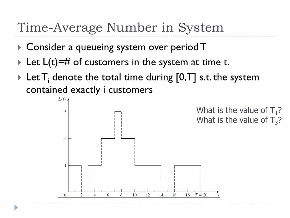
Consider a queueing system over period T
Let L(t)=# of customers in the system at time t.
Let Ti denote the total time during [0,T] s.t. the system
contained exactly i customers
What is the value of T1?What is the value of T3?
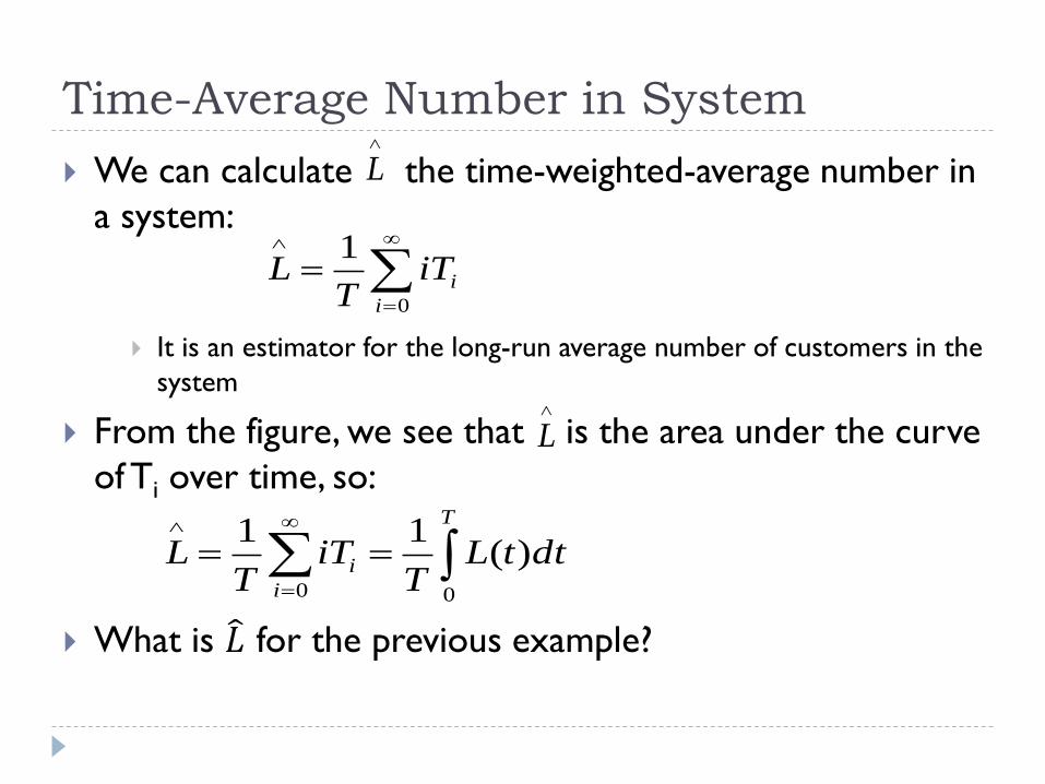
Time-Average Number in System
We can calculate the time-weighted-average number in
a system:
It is an estimator for the long-run average number of customers in the
system
From the figure, we see that is the area under the curve
of Ti over time, so:
What is 𝐿 for the previous example?
L
0
1
i
iTiT
L
L
T
i
i dttLT
TiT
L00
)(11
Time-Average Number in System
For many stable systems, as T , 𝐿 approaches L, which
is known as the long-run time-average number of customers
in the system
The estimator 𝐿 is said to be strongly consistent for L
The longer we run the simulation, the closer it gets to L
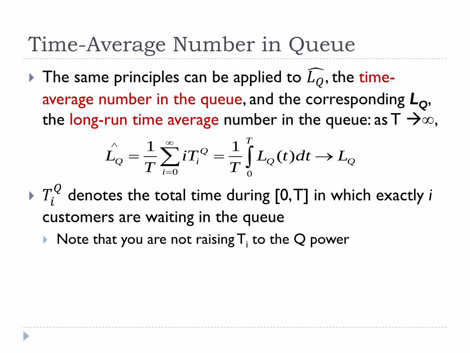
Time-Average Number in Queue
The same principles can be applied to 𝐿𝑄, the time-
average number in the queue, and the corresponding LQ,
the long-run time average number in the queue: as T ,
𝑇𝑖𝑄
denotes the total time during [0, T] in which exactly i
customers are waiting in the queue
Note that you are not raising Ti to the Q power
T
i
Q
iQ LdttLT
TiT
L00
)(11
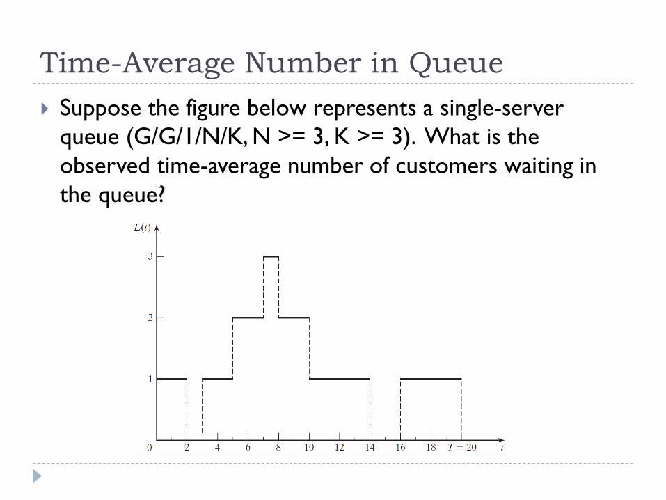
Time-Average Number in Queue
Suppose the figure below represents a single-server
queue (G/G/1/N/K, N >= 3, K >= 3). What is the
observed time-average number of customers waiting in
the queue?
Average Time Spent in the System
Let Wi be the amount of time that the ith customer spent
in the system during [0,T]. If there were N customers, the
average time spent in a system per customer is:
For stable systems, as N , 𝑤 w, where w is called the
long-run average system time
Again, similar calculations can be done for just the queue part
(i.e., estimating wQ with 𝑤𝑄)
We can think of these values as the observed delay and the long-run
average delay per customer
N
i
iWN
w1
1
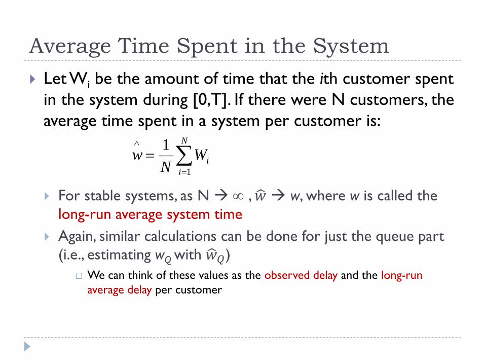
Average Time Example
How many customers arrive in the system?
22
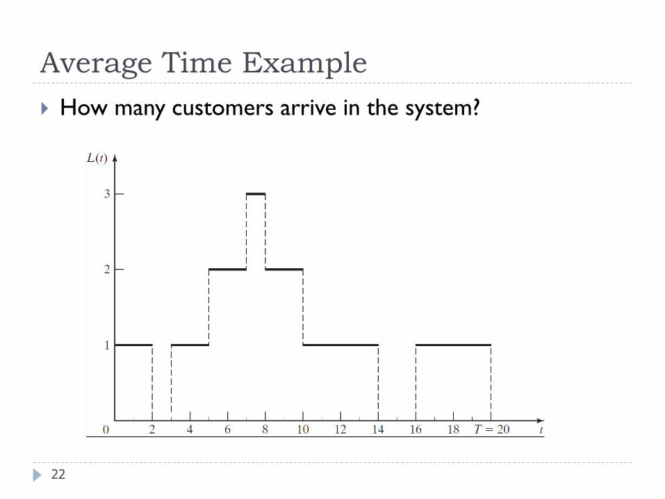
Average Time Example
What’s the total time customer 1 spent in the system
i.e. what’s W1?
What’s the total time of customer 5 (i.e. what’s W5?)
What’s the total time of customers 2, 3, 4?
24
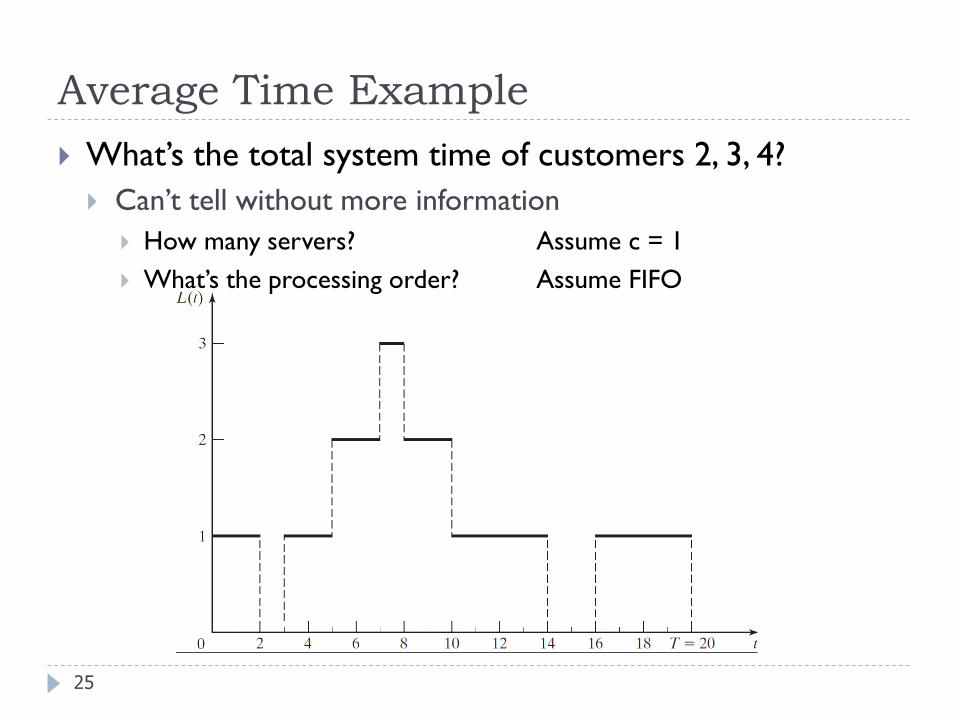
Average Time Example
What’s the total system time of customers 2, 3, 4?
Can’t tell without more information
How many servers? Assume c = 1
What’s the processing order? Assume FIFO
25
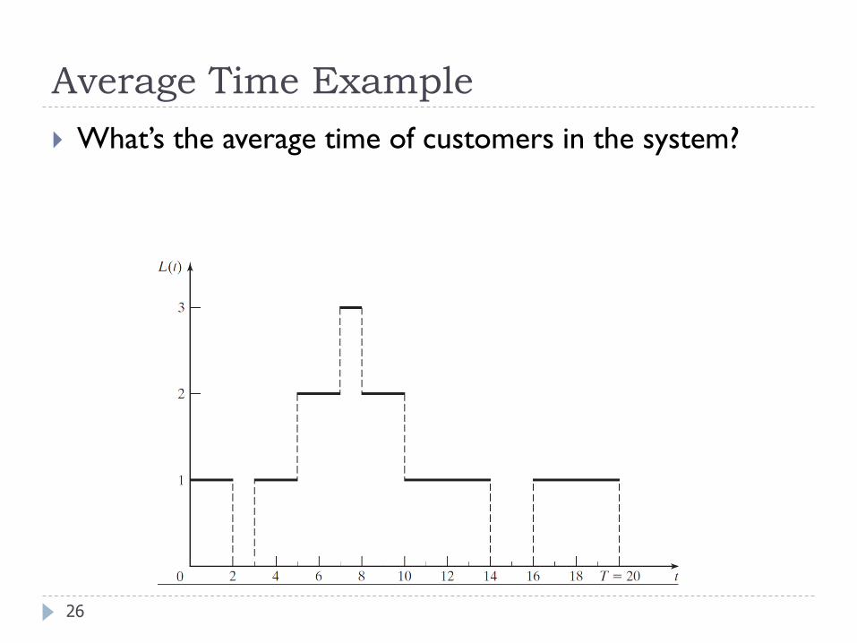
Average Time Example
What’s the average time of customers in the system?
26
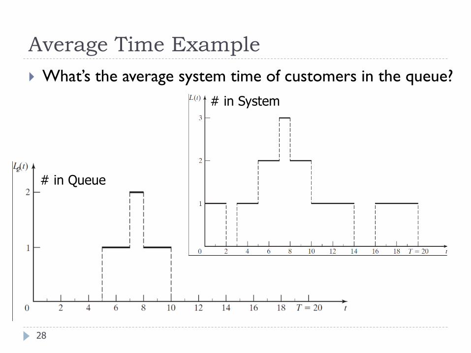
Average Time Example
What’s the average system time of customers in the queue?
28
# in Queue
# in System
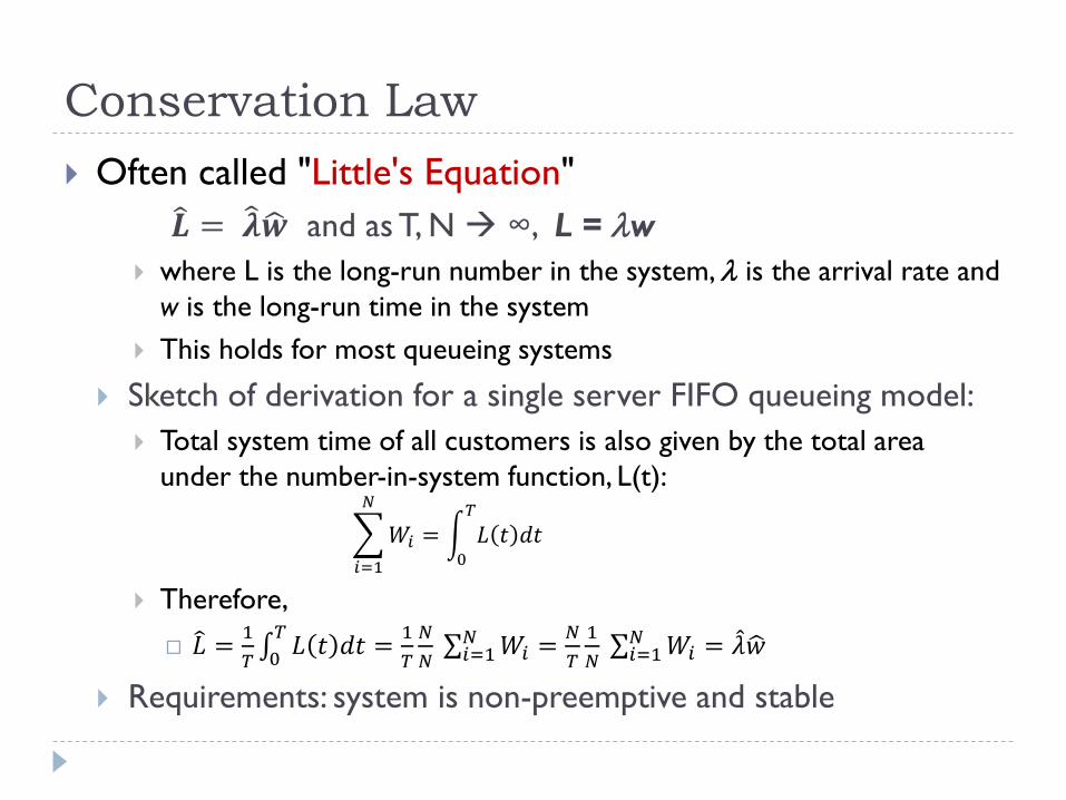
Conservation Law
Often called "Little's Equation"
𝑳 = 𝝀 𝒘 and as T, N ∞, L = w
where L is the long-run number in the system, is the arrival rate and
w is the long-run time in the system
This holds for most queueing systems
Sketch of derivation for a single server FIFO queueing model:
Total system time of all customers is also given by the total area
under the number-in-system function, L(t):
𝑖=1
𝑁
𝑊𝑖 = 0
𝑇
𝐿 𝑡 𝑑𝑡
Therefore,
𝐿 =1
𝑇 0
𝑇𝐿 𝑡 𝑑𝑡 =
1
𝑇
𝑁
𝑁 𝑖=1
𝑁 𝑊𝑖 =𝑁
𝑇
1
𝑁 𝑖=1
𝑁 𝑊𝑖 = 𝜆 𝑤
Requirements: system is non-preemptive and stable
System Stability
32
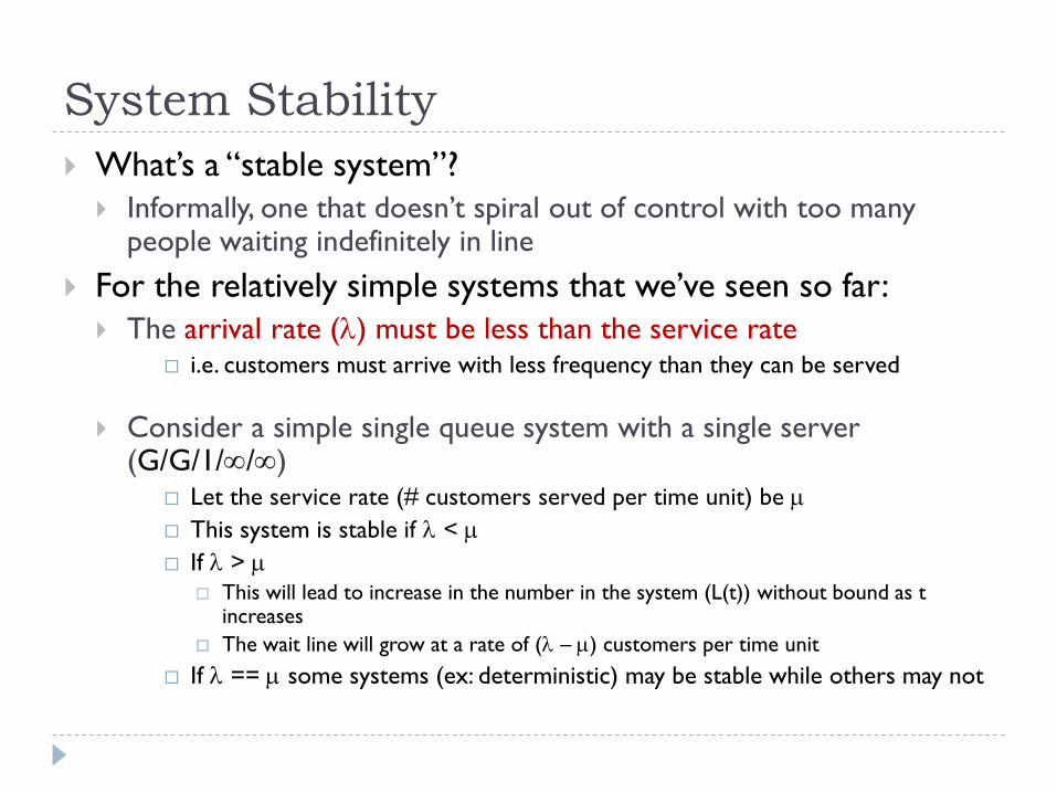
What’s a “stable system”?
Informally, one that doesn’t spiral out of control with too many people waiting indefinitely in line
For the relatively simple systems that we’ve seen so far:
The arrival rate () must be less than the service rate i.e. customers must arrive with less frequency than they can be served
Consider a simple single queue system with a single server (G/G/1//)
Let the service rate (# customers served per time unit) be
This system is stable if <
If >
This will lead to increase in the number in the system (L(t)) without bound as t increases
The wait line will grow at a rate of ( – ) customers per time unit
If == some systems (ex: deterministic) may be stable while others may not
Arrival Rates, Service Rates and Stability
33
For a system with multiple servers (ex: G/G/c//)
Stable if the net service rate of all servers together is greater
than the arrival rate
If all servers have the same rate , then the system is stable if < c
For a system with finite system capacity or calling pool
the system can be stable even if the arrival rate exceeds
the service rate
Ex: G/G/c/N/
The system is unstable until it "fills" up to N. At this point, excess arrivals
are not allowed into the system, so it is stable from that point on
Ex: G/G/c//k
With a fixed calling population, we are in effect restricting the arrival rate
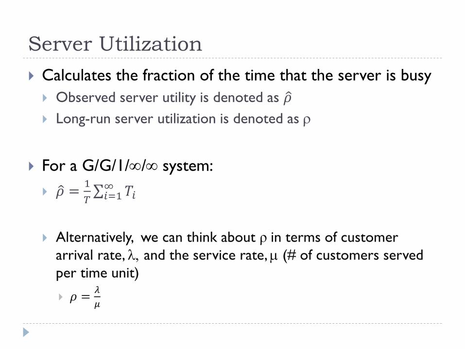
Server Utilization
Calculates the fraction of the time that the server is busy
Observed server utility is denoted as 𝜌
Long-run server utilization is denoted as
For a G/G/1// system:
𝜌 =1
𝑇 𝑖=1
∞ 𝑇𝑖
Alternatively, we can think about ρ in terms of customer
arrival rate, , and the service rate, (# of customers served
per time unit)
𝜌 =𝜆
𝜇
Server Utilization Example
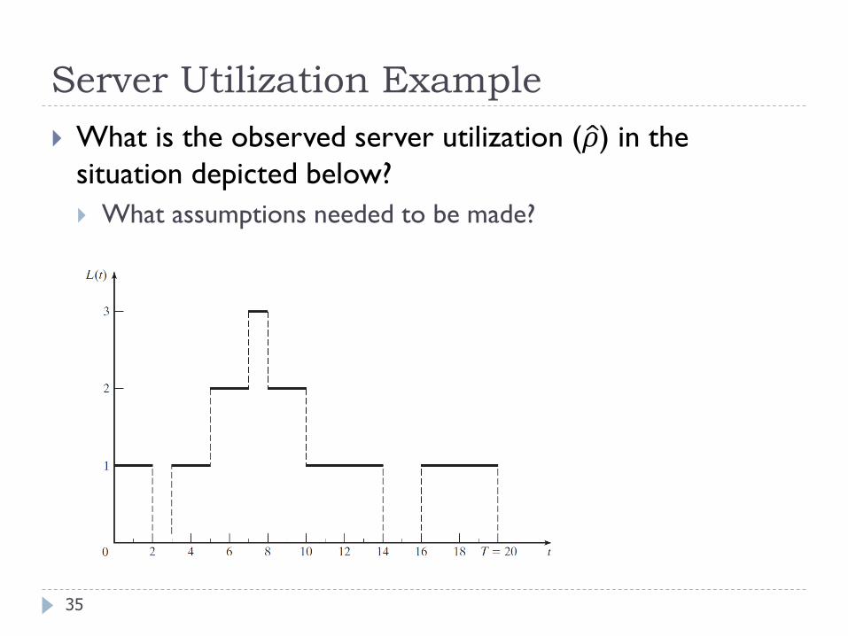
What is the observed server utilization ( 𝜌) in the
situation depicted below?
What assumptions needed to be made?
35
People waiting for a bank teller
What’s the server utilization?
Server Utilization in G/G/1/∞/∞
37 Figure fromhttp://ocw.mit.edu/courses/civil-and-environmental-engineering/1-203j-logistical-and-transportation-planning-methods-fall-2004/lecture-notes/qlec1.pdf
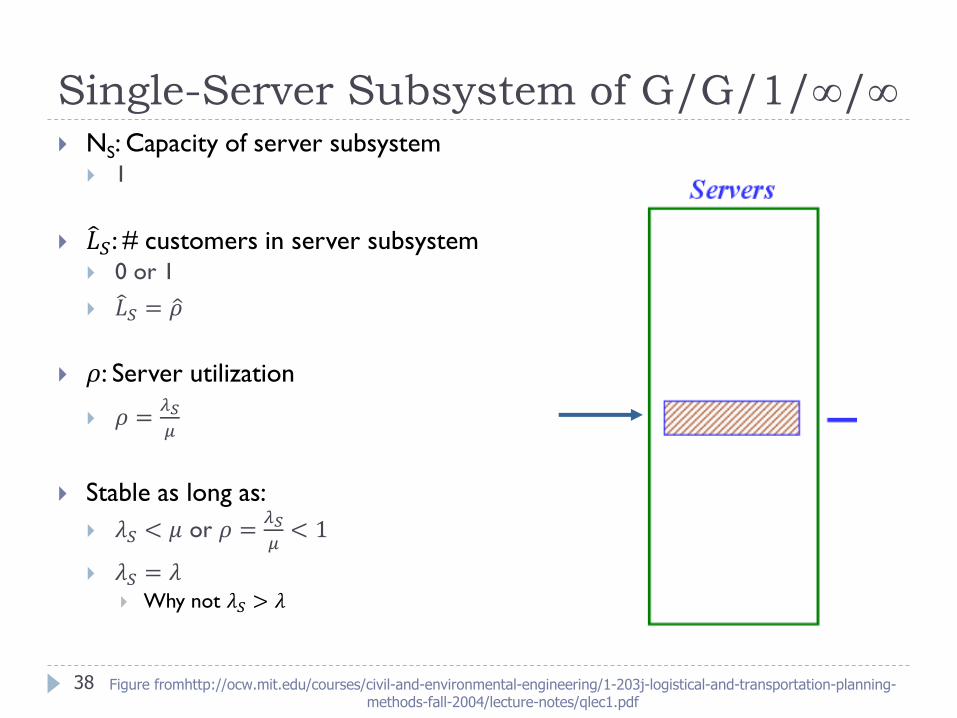
Single-Server Subsystem of G/G/1/∞/∞
38
NS: Capacity of server subsystem 1
𝐿𝑆: # customers in server subsystem 0 or 1
𝐿𝑆 = 𝜌
𝜌: Server utilization
𝜌 =𝜆𝑆
𝜇
Stable as long as:
𝜆𝑆 < 𝜇 or 𝜌 =𝜆𝑆
𝜇< 1
𝜆𝑆 = 𝜆 Why not 𝜆𝑆 > 𝜆
Figure fromhttp://ocw.mit.edu/courses/civil-and-environmental-engineering/1-203j-logistical-and-transportation-planning-methods-fall-2004/lecture-notes/qlec1.pdf
Server Utilization for G/G/1// Systems
For a single server, we can consider the server portion as
a “system” (w/o the queue)
This means Ls, the average number of customers in the "server
system,“ equals
The average system time ws is the same as the average service time
ws = 1/
From the conservation equation, we know Ls = sws
For the system to be stable, s = , since we cannot serve faster than
customers arrive and if we serve more slowly the line will grow
indefinitely
Therefore: = Ls = sws = (1/) = /
This shows: a stable queueing system must have a server
utilization of less than 1
Server Utilization for G/G/c// systems
41
Similar analysis holds for a stable system with c servers
Since the system is stable, we must have
< c
And so the server utilization generalizes to
= /c < 1
Example: Customers arrive at random to a license bureau at a rate of 50 customers/hour. Currently, there are 20 clerks, each serving 5 customers/hour on average.
What is the average server utilization?
What is the average number of busy servers?
What is the minimum # of clerks needed to keep the system stable?
Steady-State Behavior of
M/M/c/∞/∞ Systems
A queueing system is said to be in statistical equilibrium,
or steady state, if the probability that the system is in a
given state is not time dependent
e.g., the prob. of having n people in the system doesn’t depend
on time – Pr(L(t)=n) is some value Pn for all time t
For relatively simple queueing models, some of the long-
run steady state performance measures can be calculated
analytically
May enable us to avoid a simulation for simple systems
May give us a good starting point even if the actual system is
more complicated
43
Queueing Systems with Markov properties
Why is an Exponential Distribution called “Markov”?
Short answer: Has to do with its memoryless property
Markov Chains (discrete)
A set of random variables (“states”) X1, X2, … forms a Markov
Chain if the probability of transitioning from Xi to Xi+1 does not
depend on any of the previous X1, … Xi-1
Pr(Xi+1 | X1,…,Xi) = Pr(Xi+1|Xi)
Markov Process
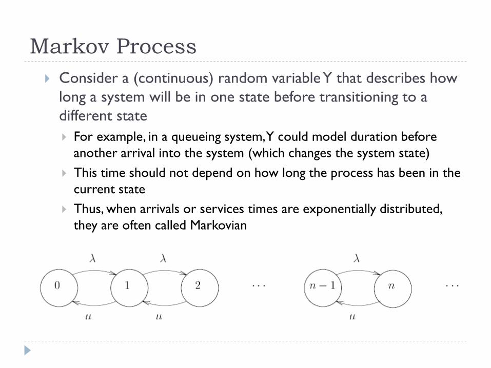
Consider a (continuous) random variable Y that describes how
long a system will be in one state before transitioning to a
different state
For example, in a queueing system, Y could model duration before
another arrival into the system (which changes the system state)
This time should not depend on how long the process has been in the
current state
Thus, when arrivals or services times are exponentially distributed,
they are often called Markovian
Steady-State Behavior of
M/M/c/∞/∞ Systems
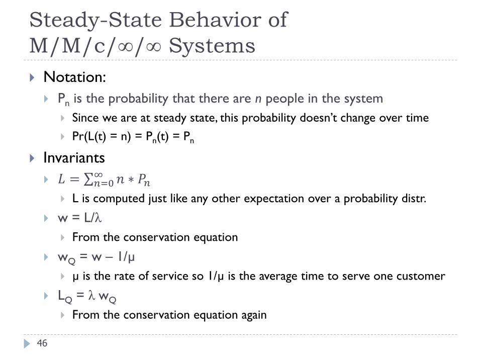
Notation:
Pn is the probability that there are n people in the system
Since we are at steady state, this probability doesn’t change over time
Pr(L(t) = n) = Pn(t) = Pn
Invariants
𝐿 = 𝑛=0∞ 𝑛 ∗ 𝑃𝑛
L is computed just like any other expectation over a probability distr.
w = L/λ
From the conservation equation
wQ = w – 1/µ
µ is the rate of service so 1/µ is the average time to serve one customer
LQ = λ wQ
From the conservation equation again
46
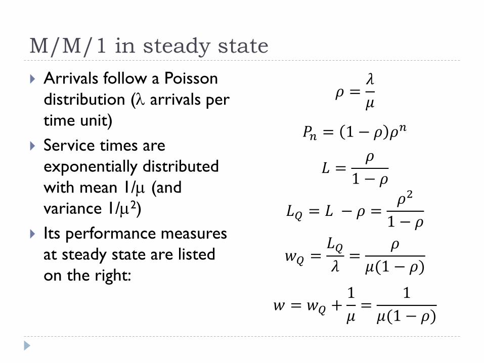
M/M/1 in steady state
Arrivals follow a Poisson
distribution ( arrivals per
time unit)
Service times are
exponentially distributed
with mean 1/ (and
variance 1/2)
Its performance measures
at steady state are listed
on the right:
𝜌 =𝜆
𝜇
𝑃𝑛 = 1 − 𝜌 𝜌𝑛
𝐿 =𝜌
1 − 𝜌
𝐿𝑄 = 𝐿 − 𝜌 =𝜌2
1 − 𝜌
𝑤𝑄 =𝐿𝑄
𝜆=
𝜌
𝜇(1 − 𝜌)
𝑤 = 𝑤𝑄 +1
𝜇=
1
𝜇(1 − 𝜌)
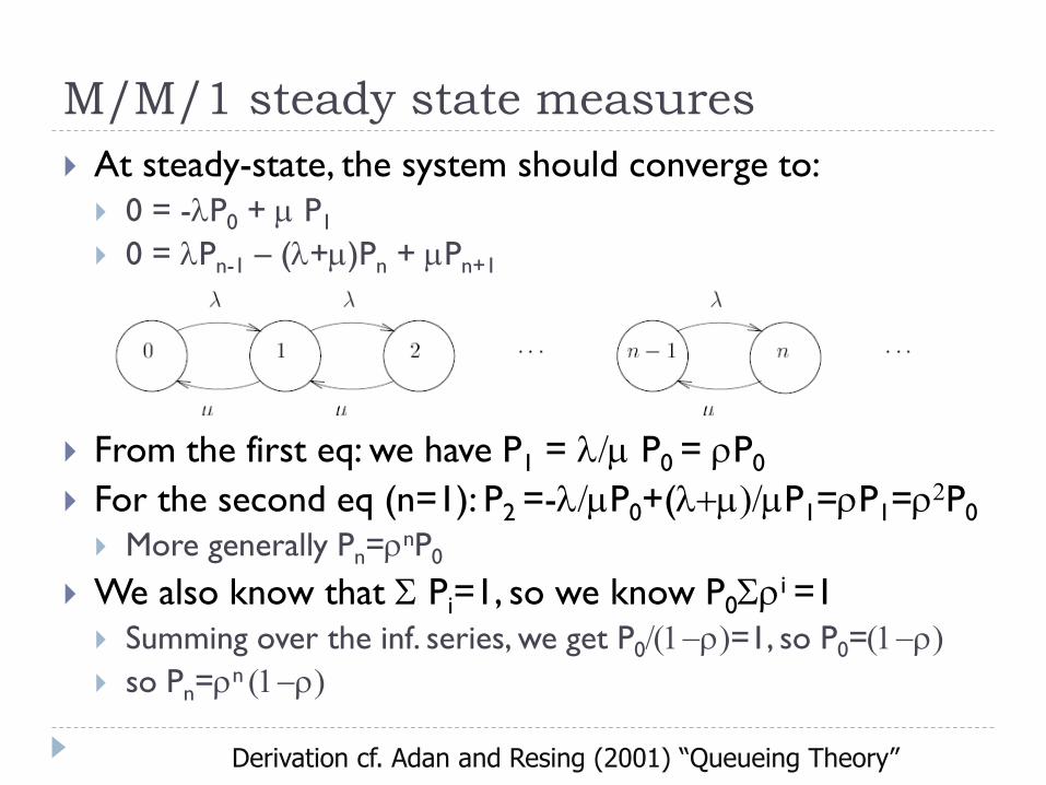
M/M/1 steady state measures
At steady-state, the system should converge to:
0 = -P0 + P1
0 = Pn-1 – (+)Pn + Pn+1
From the first eq: we have P1 = / P0 = P0
For the second eq (n=1): P2 =-/P0+(+)/P1=P1=2P0
More generally Pn=nP0
We also know that S Pi=1, so we know P0Si =1
Summing over the inf. series, we get P0/(1-)=1, so P0=(1-)
so Pn=n (1-)
Derivation cf. Adan and Resing (2001) “Queueing Theory”
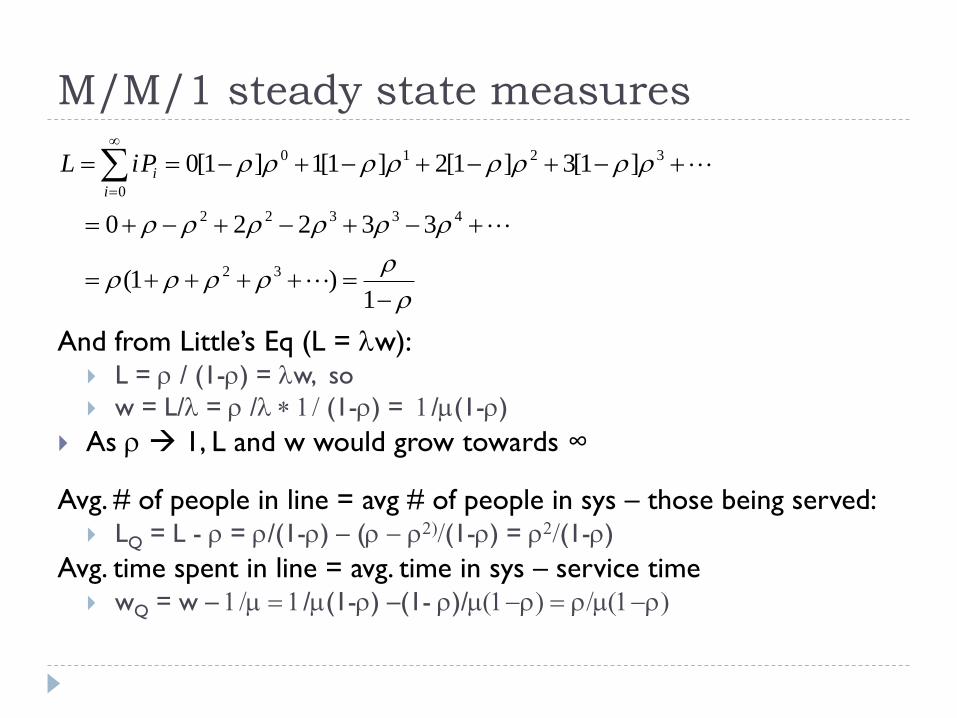
M/M/1 steady state measures
And from Little’s Eq (L = w): L = / (1-) = w, so
w = L/ = / * 1/ (1-) = 1/(1-)
As 1, L and w would grow towards ∞
Avg. # of people in line = avg # of people in sys – those being served: LQ = L - = /(1-) – ( - 2)/(1-) = 2/(1-)
Avg. time spent in line = avg. time in sys – service time wQ = w – 1/ 1/(1-) –(1- )/(1-) /(1-)
-++++
+-+-+-+
+-+-+-+-
1)1(
33220
]1[3]1[2]1[1]1[0
32
43322
3210
0
i
iPiL
M/M/1 example (adapted from ex 6.12)
Suppose the customer arrival rate is 10 per hour,
following a Poisson distribution.
You have a choice of hiring either Alice or Bob. Alice
works at a rate of 11 customers per hour, while Bob
works at a rate of 12 customers per hour. However, Bob
wants to be paid about twice as much as Alice. Should
you consider hiring Bob?
M/G/1 in Steady-State
52
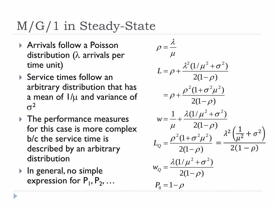
Arrivals follow a Poisson distribution ( arrivals per time unit)
Service times follow an arbitrary distribution that has a mean of 1/ and variance of s2
The performance measures for this case is more complex b/c the service time is described by an arbitrary distribution
In general, no simple expression for P1, P2, …
s
s
s
s
s
-
-
+
-
+
-
++
-
++
-
++
1
)1(2
)/1(
)1(2
)1(
)1(2
)/1(1
)1(2
)1(
)1(2
)/1(
0
22
222
22
222
222
P
w
L
w
L
Q
Q=
𝜆2 1𝜇2 + 𝜎2
2 1 − 𝜌
M/G/1 in Steady-State
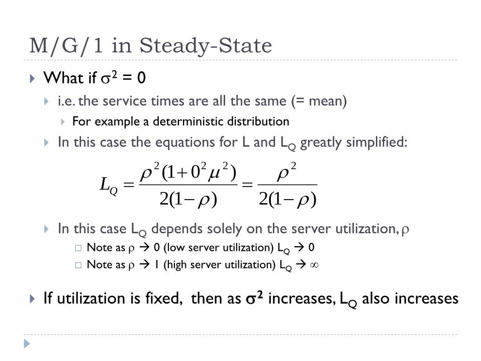
What if s2 = 0
i.e. the service times are all the same (= mean)
For example a deterministic distribution
In this case the equations for L and LQ greatly simplified:
In this case LQ depends solely on the server utilization,
Note as 0 (low server utilization) LQ 0
Note as 1 (high server utilization) LQ
If utilization is fixed, then as s2 increases, LQ also increases
)1(2)1(2
)01( 2222
-
-
+QL
M/G/1 in Steady-State
54
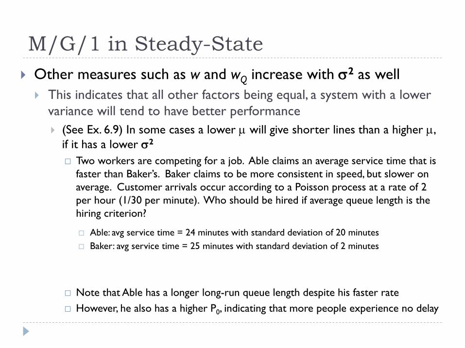
Other measures such as w and wQ increase with s2 as well
This indicates that all other factors being equal, a system with a lower
variance will tend to have better performance
(See Ex. 6.9) In some cases a lower will give shorter lines than a higher ,
if it has a lower s2
Two workers are competing for a job. Able claims an average service time that is
faster than Baker’s. Baker claims to be more consistent in speed, but slower on
average. Customer arrivals occur according to a Poisson process at a rate of 2
per hour (1/30 per minute). Who should be hired if average queue length is the
hiring criterion?
Able: avg service time = 24 minutes with standard deviation of 20 minutes
Baker: avg service time = 25 minutes with standard deviation of 2 minutes
Note that Able has a longer long-run queue length despite his faster rate
However, he also has a higher P0, indicating that more people experience no delay
Coefficient of Variation
56
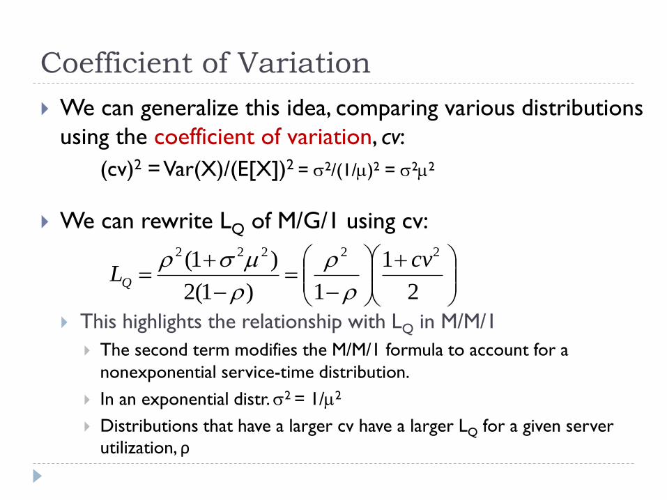
We can generalize this idea, comparing various distributions
using the coefficient of variation, cv:
(cv)2 = Var(X)/(E[X])2 = s2/(1/)2 = s22
We can rewrite LQ of M/G/1 using cv:
This highlights the relationship with LQ in M/M/1
The second term modifies the M/M/1 formula to account for a
nonexponential service-time distribution.
In an exponential distr. s2 = 1/2
Distributions that have a larger cv have a larger LQ for a given server
utilization, ρ
+
-
-
+
2
1
1)1(2
)1( 22222 cvLQ
s
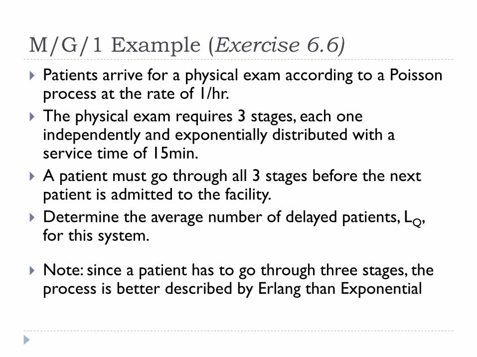
M/G/1 Example (Exercise 6.6)
57
Patients arrive for a physical exam according to a Poisson process at the rate of 1/hr.
The physical exam requires 3 stages, each one independently and exponentially distributed with a service time of 15min.
A patient must go through all 3 stages before the next patient is admitted to the facility.
Determine the average number of delayed patients, LQ, for this system.
Note: since a patient has to go through three stages, the process is better described by Erlang than Exponential
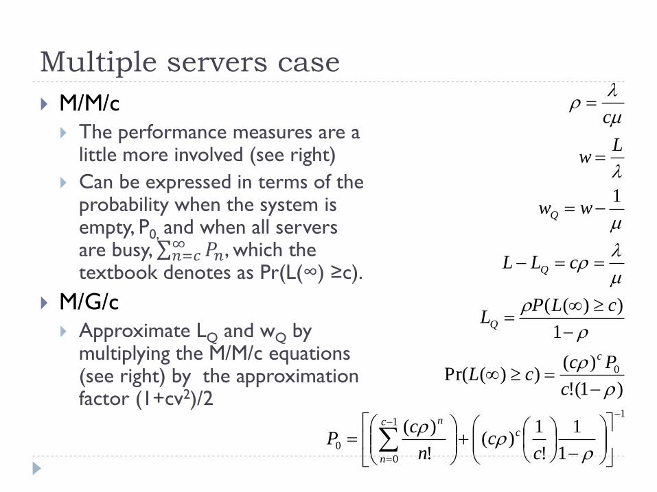
Multiple servers case
M/M/c
The performance measures are a little more involved (see right)
Can be expressed in terms of the probability when the system is empty, P0, and when all servers are busy, 𝑛=𝑐
∞ 𝑃𝑛, which the textbook denotes as Pr(L(∞) ≥c).
M/G/c
Approximate LQ and wQ by multiplying the M/M/c equations (see right) by the approximation factor (1+cv2)/2
11
0
0
0
1
1
!
1)(
!
)(
)1(!
)())(Pr(
1
))((
1
--
-
+
-
-
-
-
cc
n
cP
c
PccL
cLPL
cLL
ww
Lw
c
cc
n
n
c
Q
Q
Q
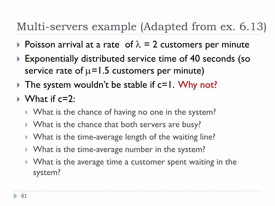
Multi-servers example (Adapted from ex. 6.13)
61
Poisson arrival at a rate of = 2 customers per minute
Exponentially distributed service time of 40 seconds (so
service rate of =1.5 customers per minute)
The system wouldn’t be stable if c=1. Why not?
What if c=2:
What is the chance of having no one in the system?
What is the chance that both servers are busy?
What is the time-average length of the waiting line?
What is the time-average number in the system?
What is the average time a customer spent waiting in the
system?
Infinite # of servers
64
Special case when c=∞
This can model self service systems
It’s appropriate for situations where service capacity far
exceeds demands
It can be used to answer the question: how many servers are
required so that customers will rarely be delayed?
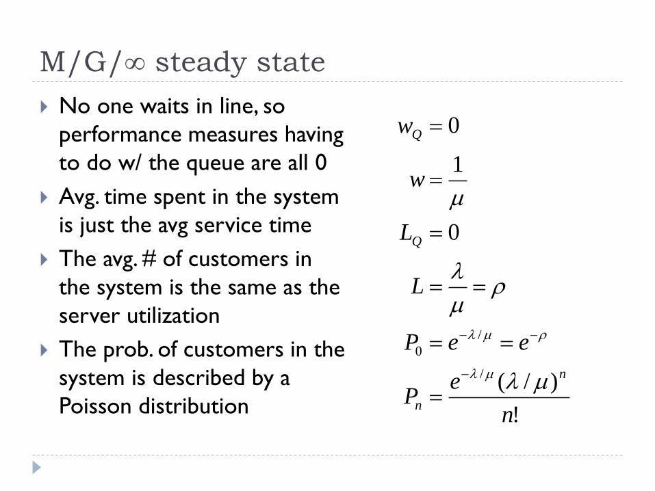
M/G/∞ steady state
No one waits in line, so
performance measures having
to do w/ the queue are all 0
Avg. time spent in the system
is just the avg service time
The avg. # of customers in
the system is the same as the
server utilization
The prob. of customers in the
system is described by a
Poisson distribution !
)/(
0
1
0
/
/
0
n
eP
eeP
L
L
w
w
n
n
Q
Q
-
--
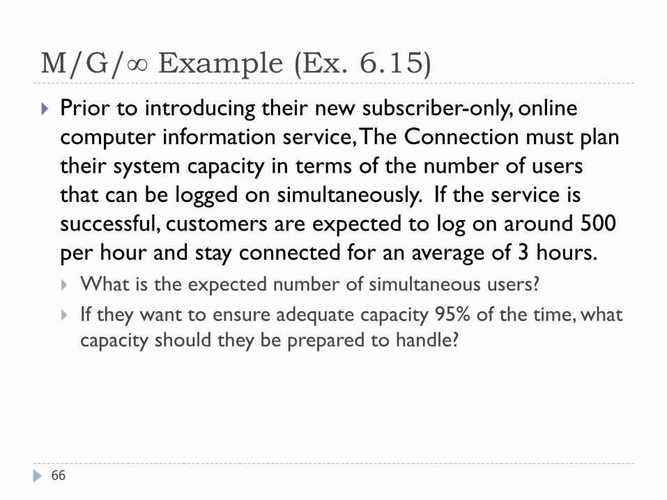
M/G/∞ Example (Ex. 6.15)
Prior to introducing their new subscriber-only, online
computer information service, The Connection must plan
their system capacity in terms of the number of users
that can be logged on simultaneously. If the service is
successful, customers are expected to log on around 500
per hour and stay connected for an average of 3 hours.
What is the expected number of simultaneous users?
If they want to ensure adequate capacity 95% of the time, what
capacity should they be prepared to handle?
66
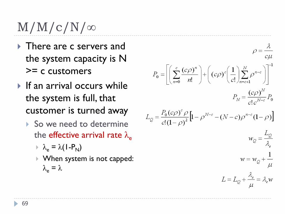
M/M/c/N/∞
There are c servers and
the system capacity is N
>= c customers
If an arrival occurs while
the system is full, that
customer is turned away
So we need to determine
the effective arrival rate λe
λe = λ(1-PN)
When system is not capped:
λe = λ
69
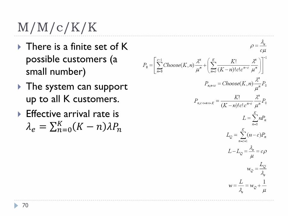
M/M/c/K/K
There is a finite set of K
possible customers (a
small number)
The system can support
up to all K customers.
Effective arrival rate is
𝜆𝑒 = 𝑛=0𝐾 𝐾 − 𝑛 𝜆𝑃𝑛
70