Queueing Theory

Peter Fenwick, July 2002

August 7, 2009

1 Preliminary note on mathematical models

Most of Computer Science has rather little contact with numbers, measurements and physicalreality – it doesn’t matter too much if things get a bit slower, or a bit faster.

Data Communications is not like that. It is full of physical quantities such as propagation veloc-ities and delays, bit rates, message lengths, and so on. With real-world things like this we oftenset up mathematical pictures or “models” to describe and predict behaviour.

Now all three of the 742 lecturers (in 2001 at least) have a background in Physics, and Physics islargely about finding mathematical models or descriptions of some physical system or process.This means that we often work in terms of models, sometimes without even realising it, and thiscan lead to all sorts of confusions among Computer Science students. The queueing theory ofthese notes leads to quite typical mathematical models, with hidden or assumed implications.

Some of these aspects are –

1. A model is never any more than an approximation to reality; people can all to easily assumethat their model is reality and then get into all sorts of problems. Sometimes a simple modelexists only because we can’t handle the mathematics of a more accurate one! This oftenapplies to queueing theory.

2. When using a model you must know what simplifications and assumptions it makes. Forexample a very simple model of the flight of a ball or other projectile says that it is a parabola.More complex models progressively introduce air resistance, the spin of the ball, the rotationof the earth and even more, but at increasing complexity.

3. You must recognise the limitations of the model, when it works and when it doesn’t. Know-ing when it will not predict is at least important as knowing when it will predict.

4. You may find that somebody used to working with models will assume one for a while andthen abruptly abandon it or move to another, when the original one is “clearly inappropri-ate”. If you understand the model and its limitations as in the earlier points, the changemay be natural. If you do not understand those aspects, it is totally confusing. Be warned –I have found this can be a very real problem!

5. Sometimes you can use a very simple, crude, model to see if something is feasible. For ex-ample if a communications protocol must transfer data at 1.5Mbit/s, and “quick and dirty”

1

calculation shows that it can never do better than 1.1Mbit/s then you probably need anotherapproach. But if that calculation showed that it should work at 1.6 or even 1.4 Mbit/s thena more careful calculation is probably justified.

2 Queueing Theory – Introduction and Terms

Queueing Theory deals with the situation where customers(people, or other entities) wait in anordered line or queue for service from one or more servers. Customers arrive on the queue ac-cording to some assumed distribution of interarrival times and, after waiting, take some servicetime to have the request satisfied. Within the environment of a computing system, queues applyto buffers in a communication system, the handling of I/O traffic (and especially disk traffic), topeople awaiting access to a terminal, and failure rates and times to repair. In many cases therewill be several cascaded queues,or several interacting queues. Several terms must be specifiedbefore we can discuss a general queueing system –

Source The population source may be finite or infinite. The essential point of a finite population isthat the queue absorbs potential customers as it grows and the arrival rate falls in accordancewith the population not in the queue. For a large population we often assume an infinitepopulation to simplify the mathematics.

Arrival Process Assume that customers enter the queue at times t0 < t1 < t2 . . . tn . . .. The ran-dom variables τk = tk−tk−1 ( for k ≥ 1) are the interarrival times, and are assumed to form asequence of independent and identically distributed random variables. The arrival processis described by the distribution function A of the interarrival time A(t) = P [τ ≤ t].

• If the interarrival time distribution is exponential (ie P [t ≤ τ ] = 1 − e − λt, whereλ = 1/τ ), the probability of n arrivals in a time interval of length t is e−λt(λt)n/n!,for n = 0, 1, 2, . . . and the average arrival rate is λ. This corresponds to the importantcase of a Poisson distribution where, in a very large population of n customers, theprobability, P , of a particular customer entering the queue within a short time intervalis very small, but there is a reasonable probability (nP ) that some customer will arrive.

• Another important distribution is the Erlang-k distribution, defined by

Ek(x) = 1 −j=0∑

k−1

(λx)j

j!e−λx

It applies to a cascade of servers with exponential distribution times, such that a cus-tomer cannot be started until the previous one has been completely processed.

Service Time Distribution Let sk be the service time required by the kth arriving customer; as-sume that the sk are independent, identically distributed random variables and that we canrefer to an arbitrary service time as s, distributed as Ws(t) = P [s ≤ t]. The most usualservice-time distribution is exponential, defining a service called random service. If µ is theaverage service rate, then Ws(t) = 1 − e−µt.

2

Maximum queueing system capacity In some systems the queue capacity is assumed to be in-finite; all arriving customers can be accommodated, although the waiting time may be ar-bitrarily long. In others the queue capacity is zero (the customer is turned away if there isno free server). In other cases the queue may have a finite capacity, such as a waiting roomwith limited seating.

Number of servers The simplest queueing system is the single server system, which can serveonly one customer at a time. A multiserver system has c identical servers and can serve upto c customers simultaneously.

Queue discipline The queue discipline, or service discipline, defines the rule for selecting thenext customer. The most usual one is “first come first served” (FCFS), also known as “firstin first out” or FIFO. Another one is “random selection for service” (RSS) or “service inrandom order” (SIRO). In some circumstances we deal with priority queues (essentiallyparallel queues where there is a preferred order of selecting customers for service), or withpreemptive queues in which a new customer can interrupt a customer being served.

Traffic Intensity The traffic intensity ρ is the ratio of the mean service time E[s] to the meaninterarrival time E[τ ], for an arrival rate λ and service rate µ; it defines the minimum numberof servers to cope with the arriving traffic.

ρ =E[s]

E[t]= λE[s] =

λ

µ

Server utilisation The traffic intensity per server or server utilisation u = ρ/c is the approximateprobability that a server is busy (assuming that traffic is evenly divided among the servers).Note that some authors interchange ρ and u so that ρ is the server utilisation and u is thetraffic intensity – with single server systems the two have the same value.

A queue may be specified by the Kendall notation, of the form

A/B/c/K/m/Z

Here A specifies the interarrival time distribution, B the service time distribution, c the numberof servers, K the system capacity, m the number in the source, and Z the queue discipline. Theshorter notation A/B/c is often used for no limit on queue size, infinite source, and FIFO queuediscipline. The symbols used for A and B are –

GI General independent interarrival time

G General service time, usually assumed independent

Ek Erlang-k time distribution

M Exponential time distribution (Markov, or random times)

D Deterministic or constant interarrival or service time

3

mean arrival rate λmean service rate/server µmean interarrival time t = 1/λnumber of servers ctime in queue qtime at server saverage time in queue E[q]average time at server E[s]

traffic intensity ρ = λE[s] =λ

µ

per-server utilisation u =λ

cµ=

ρ

c

time in system (queue+server) w = q + s

mean time in (queue+server) W = E[w] = E[q] + E[s]

Number in queueing system N = Nq + Ns

Mean number in system L = E[N ] = λW = E[Nq] + E[Ns]

Mean number in queue Lq = λWq

Table 1: Important Relations

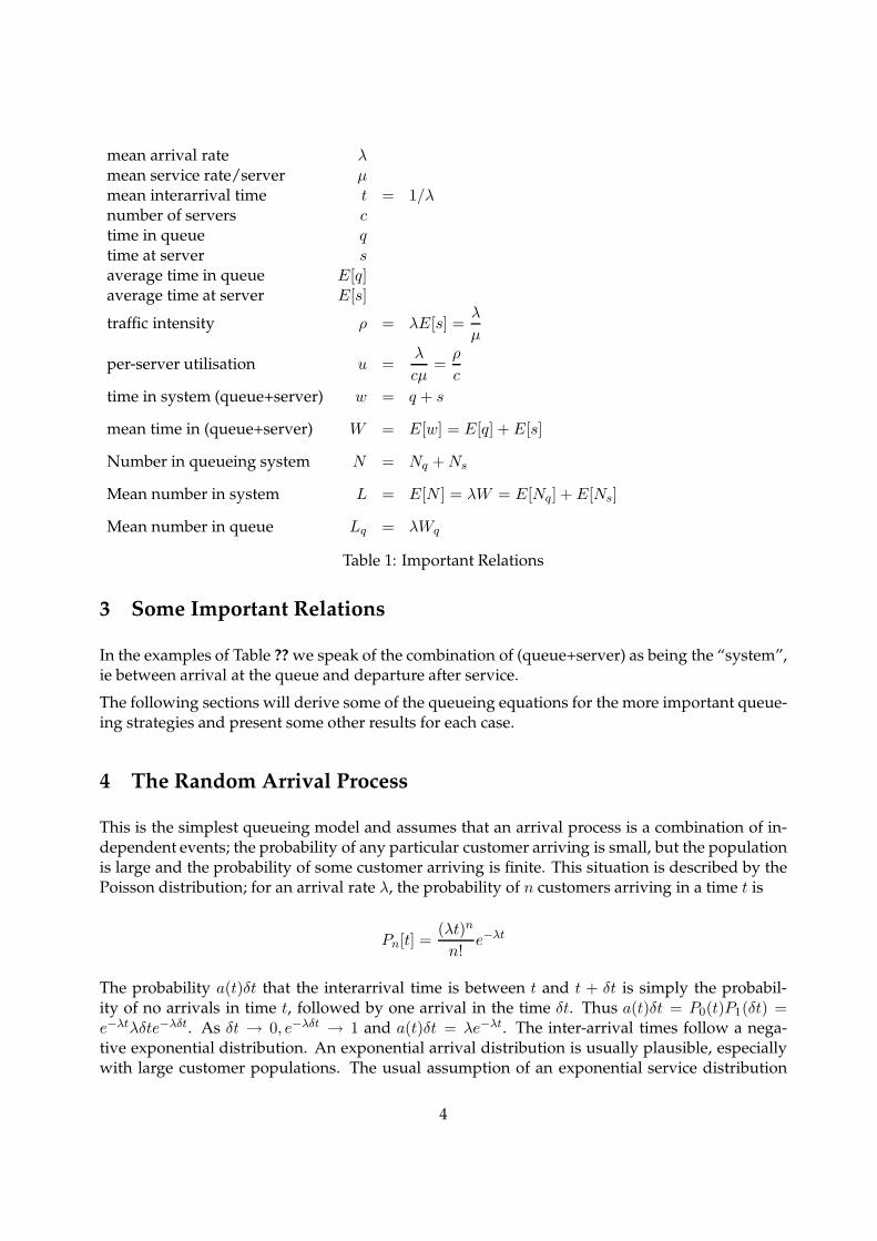
3 Some Important Relations

In the examples of Table ?? we speak of the combination of (queue+server) as being the “system”,ie between arrival at the queue and departure after service.

The following sections will derive some of the queueing equations for the more important queue-ing strategies and present some other results for each case.

4 The Random Arrival Process

This is the simplest queueing model and assumes that an arrival process is a combination of in-dependent events; the probability of any particular customer arriving is small, but the populationis large and the probability of some customer arriving is finite. This situation is described by thePoisson distribution; for an arrival rate λ, the probability of n customers arriving in a time t is

Pn[t] =(λt)n

n!e−λt

The probability a(t)δt that the interarrival time is between t and t + δt is simply the probabil-ity of no arrivals in time t, followed by one arrival in the time δt. Thus a(t)δt = P0(t)P1(δt) =e−λtλδte−λδt. As δt → 0, e−λδt → 1 and a(t)δt = λe−λt. The inter-arrival times follow a nega-tive exponential distribution. An exponential arrival distribution is usually plausible, especiallywith large customer populations. The usual assumption of an exponential service distribution

4

is usually questionable and is often defensible only on the grounds that a solution is otherwiseimpossible.

An underlying assumption is that the random arrival model has no memory; each arrival (orservice) is a separate event which is independent of what has happened before. The probabilityof its occurrence is independent of the time which that customer was away from the system orwas being serviced. In contrast, for the important case of a constant or deterministic service timethe probability of service completion is mostly zero except for one time since service commenced– the system has memory and the mathematics is far more complex, if it is indeed possible.

5 Single Server Model M/M/1,

or M/M/1/∞/∞/FIFO

This model assumes exponential interarrival and service time distributions, a single server, andno limit on queue lengths. For this case the traffic intensity ρ is equal to the server utilisation u.

Consider a queueing system with an arrival rate λ, service rate µ, and a probability Pj(t) of havingj customers (including that being served at time t). We may represent the system by a statediagram where state j corresponds to having j customers in the system. Movement between thestates is by customers arriving (moving to a “higher” state), or completing service (moving to a“lower” state). For the present assume that the arrival and service rates, λ and µ, are independentof the state. Later models do not have this simplification. [A subtle point is that the arrival andservice rates are assumed to be constant (in the steady state) so that a state transition is an independentevent, which does not depend on the time spent in the state; this condition is satisfied only for randomarrivals, or exponentially distributed inter-arrival times.] Note also that ΣPk = 1. The steady statesolution must be averaged over a time which is large compared with both of 1/λ and 1/µ. Thestate Sk corresponds to the queueing system containing k customers and occurs with a probabilityPk.

����

����

����

����- - - -

� � � �0 1 2 3

λP0 λP1 λP2 λP3

µP1 µP2 µP3 µP4

Consider first the two states S0 (empty system) and S1 (a single customer). The state moves fromS0 to S1 by a customer arriving, and the change occurs with frequency λP0. Similarly the statemoves from S1 to S0 by the customer completing service, and the change occurs with frequencyµP1. In equilibrium the two must be equal and

λP0 = µP1

Considering the probabilities of entering and leaving S1, we have that

λP0 + µP2 = µP1 + λP1

But as λP0 = µP1, we have λP1 = µP2 and in general λPk = µPk+1. Setting ρ = λ/µ, and solvingin turn for each Pk, we find that

Pk = ρkP0

5

These probabilities must total 1, giving

∞∑

k=0

ρkP0 = 1

As P0 is the probability that the system is idle and ρ is the probability that the system is busy, it isclear that P0 = 1 − ρ. Using the sum of a geometric series, we then find that

Pk = (1 − ρ)ρk

The mean number of customers in the system, N , is then

N =∞∑

k=0

kPk = (1 − ρ)∞∑

k=0

kρk

From which N = ρ1−ρ (number in system)

As the average number actually being served is ρ, the average num-ber waiting in the queue is N − ρ,giving Lq = ρ

1−ρ − ρ

= ρ2

1−ρ (number in queue)

A very important result which is intuitively obvious, but very hardto prove for the general case, is “Little’s formula”. This states that ifthe N customers are in the system for an average time T ,

then N = λT ( Little’s formula )

As the number waiting is Lq = ρ2

1−ρ ,

the time spent waiting is Wq =Lq

λ

= ρ1−ρ

λµ

1λ

= ρ1−ρ

1µ (time in queue)

Average time in the system W = Nλ = ρ

1−ρ1λ

multiplying by µ W = 1µ−λ (time in system)

Some basic results for the M/M/1 queue are shown in Table ??

6 Scaling Effect

An important phenomenon in queueing systems is the “scaling effect”. It may be assumed that ifwe have a single computer shared among n users, and replace it with n computers, each of 1/n

6

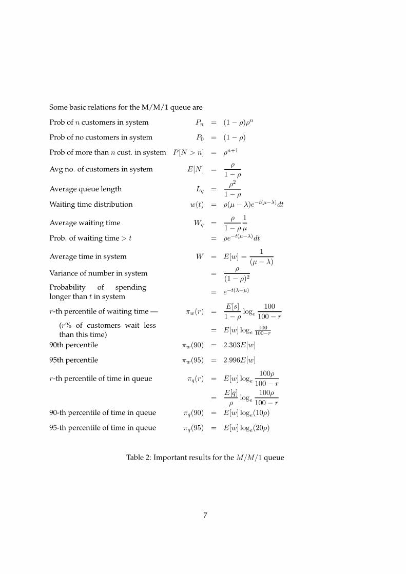
Some basic relations for the M/M/1 queue are

Prob of n customers in system Pn = (1 − ρ)ρn

Prob of no customers in system P0 = (1 − ρ)

Prob of more than n cust. in system P [N > n] = ρn+1

Avg no. of customers in system E[N ] =ρ

1 − ρ

Average queue length Lq =ρ2

1 − ρ

Waiting time distribution w(t) = ρ(µ − λ)e−t(µ−λ)dt

Average waiting time Wq =ρ

1 − ρ

1

µ

Prob. of waiting time > t = ρe−t(µ−λ)dt

Average time in system W = E[w] =1

(µ − λ)

Variance of number in system =ρ

(1 − ρ)2

Probability of spendinglonger than t in system

= e−t(λ−µ)

r-th percentile of waiting time — πw(r) =E[s]

1 − ρloge

100

100 − r(r% of customers wait lessthan this time)

= E[w] loge100

100−r

90th percentile πw(90) = 2.303E[w]

95th percentile πw(95) = 2.996E[w]

r-th percentile of time in queue πq(r) = E[w] loge

100ρ

100 − r

=E[q]

ρloge

100ρ

100 − r

90-th percentile of time in queue πq(90) = E[w] loge(10ρ)

95-th percentile of time in queue πq(95) = E[w] loge(20ρ)

Table 2: Important results for the M/M/1 queue

7

the power, that the overall response time is unchanged and we have more conveniently locatedcomputers. This plausible argument is wrong.

Assume that we have old values of λ and µ, and new values of λ/n and µ/n, then the expectedtimes in queue and times in system are –

Old time in queue E[q]old = ρµ

11−ρ

New time in queue E[q]new = ρµ/n

11−ρ

= n ρµ

11−ρ

Old time in system E[w]old = 1µ

11−ρ

New time in system E[w]new = 1µ/n

11−ρ

= n 1µ

11−ρ

The mean number waiting in the queue and the mean number waiting in the system are un-changed, but we find that

E[q]new

E[q]old=

E[w]new

E[w]old= n

The waiting times have therefore increased in inverse ratio to the computer power. The generalrule is that separate queues to slower servers should be avoided where possible. It is better tohave a single fast server.

7 Example of an M/M/1 situation

An office has one workstation which is used by an average of 10 people per 8-hour day, with theaverage time spent at the workstation exponentially distributed, and a mean time of 30 minutes.Assume an 8-hour day.

The arrival rate is λ = 10 per day = 1/48 per minute, giving a server utilisation of ρ = 30/48 =0.625; the workstation should therefore be idle for 37.5% of the time.

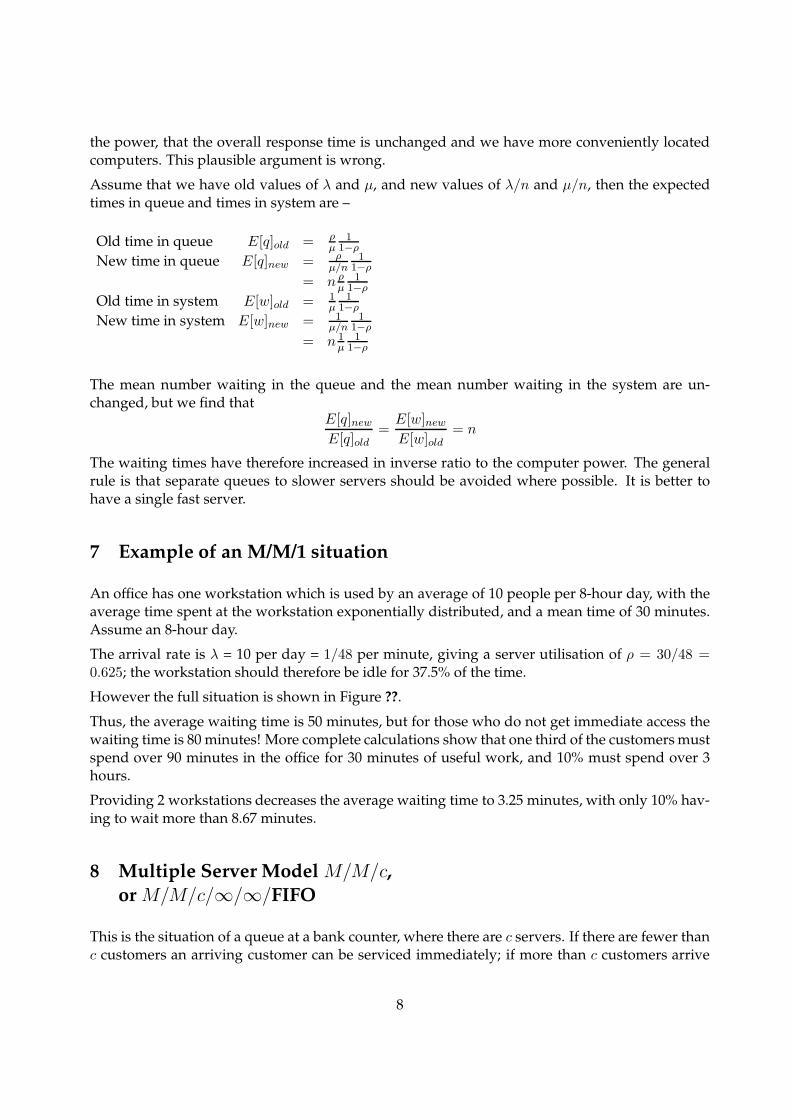
However the full situation is shown in Figure ??.

Thus, the average waiting time is 50 minutes, but for those who do not get immediate access thewaiting time is 80 minutes! More complete calculations show that one third of the customers mustspend over 90 minutes in the office for 30 minutes of useful work, and 10% must spend over 3hours.

Providing 2 workstations decreases the average waiting time to 3.25 minutes, with only 10% hav-ing to wait more than 8.67 minutes.

8 Multiple Server Model M/M/c,

or M/M/c/∞/∞/FIFO

This is the situation of a queue at a bank counter, where there are c servers. If there are fewer thanc customers an arriving customer can be serviced immediately; if more than c customers arrive

8

Probability of morethan 1 customer insystem

P [N ≥ 2] = ρ2 = 0.391

Mean steady-statenumber in system

L = E[N ] =ρ

1 − ρ

=0.625

1 − 0.625= 1.667

Mean time customerspends in system

W = E[w] =1

µ − λ= 80 minutes

Mean number of cus-tomers in queue

Lq =ρ2

1 − ρ= 1.04

Mean length of non-empty queue

E[Nq | Nq > 0] =1

1 − ρ= 2.67

Mean time in queue E[q] = 50 minutes

Mean time in queue forthose who wait

E[q | q > 0] = E[w] = 80 minutes

Figure 1: Example of M/M/1 Queueing system

they must wait for the next available server. The analysis follows the general approach takenearlier for the M/M/1 queue.

Assuming that all c servers are identical, with service rate µ, we have as before that λP0 = µP1.Considering now the transitions between P1 and P2, the “upward” rate is governed entirely bythe arrival statistics and is still λP1, but with two servers active in the P2 state, the “downward”probability is now doubled; the equation is now λP1 = 2µP2. In general, we have that λPk−1 =kµPk, for all values of k up to c (while there is no waiting queue and all arrivals can be servicedimmediately). Beyond that all servers are busy, the input queue builds up and the downward rateremains at cµ.

Solving for Pj gives Pj = 1j!

(

λµ

)jP0 for j = 0, 1, . . . , c

or, letting ρ = λ/µ Pj = ρj

j! P0 if not all servers are busy

The states when all c servers are busy may be modelled as a queue with arrival rate λ and servicerate cµ. If state c, with no customers waiting but all servers busy, occurs with probability Pc, then0, 1, 2, 3, . . . customers will be queued with probabilities

Pc,

(

λ

cµ

)

Pc,

(

λ

cµ

)2

Pc,

(

λ

cµ

)3

Pc, . . .

9

and a total probability ofPc

1 − λ/cµ= P0

ρc

c!

1

1 − λ/cµ

=ρc

c!

cµ

cµ − λP0

By normalising, we get1

P0=

c−1∑

j=0

ρj

j!+

ρc

c!

cµ

cµ − λ

If c ≫ ρ, this is nearly the series expansion for the exponential function, giving P0 = e−ρ, and

Pj =ρj

j!e−ρ

More usually, c is finite and the approximation is inappropriate, giving

Pj −ρj/j!∑

ρi/i!

Summarising the important formulae for the M/M/c system –

Probability of no cus-tomers in system

1

P0=

c−1∑

j=0

ρj

j!+

ρc

c!

cµ

cµ − λ

Probability of n cus-tomers in system

Pn = P0ρn

n!if n ≤ c

Pn = P0ρc(λ/cµ)n−c

c!if n ≥ c

Average no. in queue Lq =P0λµρc

(c − 1)!(cµ − λ)2

Average no. in system L = Lq + λ/µ

Average waiting time Wq = P0µρc

(c − 1)!(cµ − λ)2

Average time in system W = Wq + 1/µ

Waiting time distribution Wq(t)dt =P0cρ

c

c!e−(cµ−λ)tdt

Prob of waiting longer than t =P0cρ

c

c!(cµ − λ)e−(cµ−λ)t

9 Solution of the general queueing equations

In the more general case, λ and µ may depend on the state (for example, in a finite populationλ must decrease as each customer enters the queue and increase as each customer completesservice). The argument follows the line of the earlier cases, but is rather more complex. Rememberthough that the earlier restriction still applies – within a given state, the values of λ and µ mustbe independent of the time already spent in that state.

10

����

����

����

����- - - -

� � � �0 1 2 3

λ0P0 λ1P1 λ2P2 λ3P3

µ1P1 µ2P2 µ3P3 µ4P4

Consider the equilibrium conditions for state j. State j is entered at rate λj−1Pj−1 by arrivals fromstate (j − 1) and at rate µj+1Pj+1 by completion from state (j + 1). State j is left at rate λjPj byarrivals and at rate µjPj by departures. The general equilibrium condition is then

λj−1Pj−1 − (λj + µj)Pj + µj+1Pj+1 = 0

For an empty queue, λ−1 = µ0 = 0, and

0 = −λ0P0 + µ1P1

P1 =λ0

µ1P0

and, in general Pj+1 =λj + µj

µj+1Pj −

λj−1

µj+1Pj−1

whence, substitutingfor values of j,

Pj =λ0λ1 . . . λj−1

µ1µ2 . . . µjP0

=λ0

µj

j−1∏

i=0

λi

µiP0

As the sum over all j =1, we get

1

P0= 1 +

λ0

µ1+

n∑

j=2

λ0

µ1

j−1∏

i=1

λi

µi

The mean queue lengthL is then

L =∑

jPj

=

[

λ0

µ1+ 2

λ0λ1

µ1µ2+ 3

λ0λ1λ2

µ1µ2µ3+ . . .

]

P0

Note that this equation is quite general – it relates the queue sizes to the arrival rates λ and servicerates µ. We can get different queueing models by choosing different behaviours for the λ and µ. Inmost cases µ will be independent of the queue size (although the M/M/c queue can regarded as acase with varying µ), but for a finite population we may find that λ decreases as customers enterthe queue. Similarly, if customers are deterred by a long queue, we may find that λ decreases forlarge queues. The special case of multiple servers has been dealt with already, and another one isdescribed in the next section. Other situations can be handled, provided only that the values of λand µ can be calculated.

11

10 The Machine-repair model M/M/1/k/k/FIFO

(or Machine-interference model)

The machine-repair is an extreme example of a finite population queueing system; the entirepopulation may be in the system and the arrival rate zero. Some examples are –

• a machine-shop with a number of machines which work for a while and then need attention;the time to failure follows an exponential distribution (surprise!). A single maintenanceworker has the job of repairing the failed machines; the repair time is again exponentiallydistributed. (The machine-repair model is an extreme case of a finite-population queueingsystem.) This model yields the extremely important concept of “walk time”, which ariseswhen a service worker (or computer, etc) visits or examines units in sequence. The walk timeis the time to move from one unit to the next and is essentially non-productive or wastedtime.

• a multi-processor computer with a shared memory. The processors work for a time beforethey need data from the memory (ie they “fail”) and enter the memory queue for “servic-ing”. They then resume operation as soon as the shared memory responds.

• a small population of users of a computer, where each user does other work for a while andthen queues for the computer, thus removing one potential computer user.

• a polled or sequential access computer network where users work preparing input and thenneed service from the central computer (ie they “fail”) and the computer polls or visits eachin turn.

• A client-server system, where clients make requests of a central server and must wait for theresponse before they can proceed.

����

����

����

����- - - -

� � � �0 1 2 3

kλ0P0 (k − 1)λ1P1 (k − 3)λ2P2 (k − 4)λ3P3

µP1 µP2 µP3 µP4

12

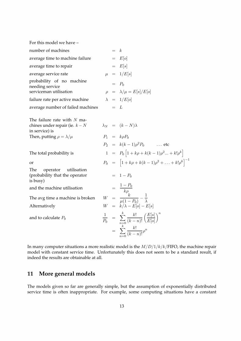
For this model we have –

number of machines = k

average time to machine failure = E[o]

average time to repair = E[s]

average service rate µ = 1/E[s]

probability of no machineneeding service

= P0

serviceman utilisation ρ = λ/µ = E[s]/E[o]

failure rate per active machine λ = 1/E[o]

average number of failed machines = L

The failure rate with N ma-chines under repair (ie. k−Nin service) is

λN = (k − N)λ

Then, putting ρ = λ/µ P1 = kρP0

P2 = k(k − 1)ρ2P0 . . . etc

The total probability is 1 = P0

[

1 + kρ + k(k − 1)ρ2... + k!ρk]

or P0 =[

1 + kρ + k(k − 1)ρ2 + . . . + k!ρk]

−1

The operator utilisation(probability that the operatoris busy)

= 1 − P0

and the machine utilisation =1 − P0

kρ

The avg time a machine is broken W =k

µ(1 − P0)−

1

λAlternatively W = k/λ − E[o] − E[s]

and to calculate P01

P0=

k∑

n=0

k!

(k − n)!

(

E[s]

E[o]

)n

=k∑

n=0

k!

(k − n)!ρn

In many computer situations a more realistic model is the M/D/1/k/k/FIFO, the machine repairmodel with constant service time. Unfortunately this does not seem to be a standard result, ifindeed the results are obtainable at all.

11 More general models

The models given so far are generally simple, but the assumption of exponentially distributedservice time is often inappropriate. For example, some computing situations have a constant

13

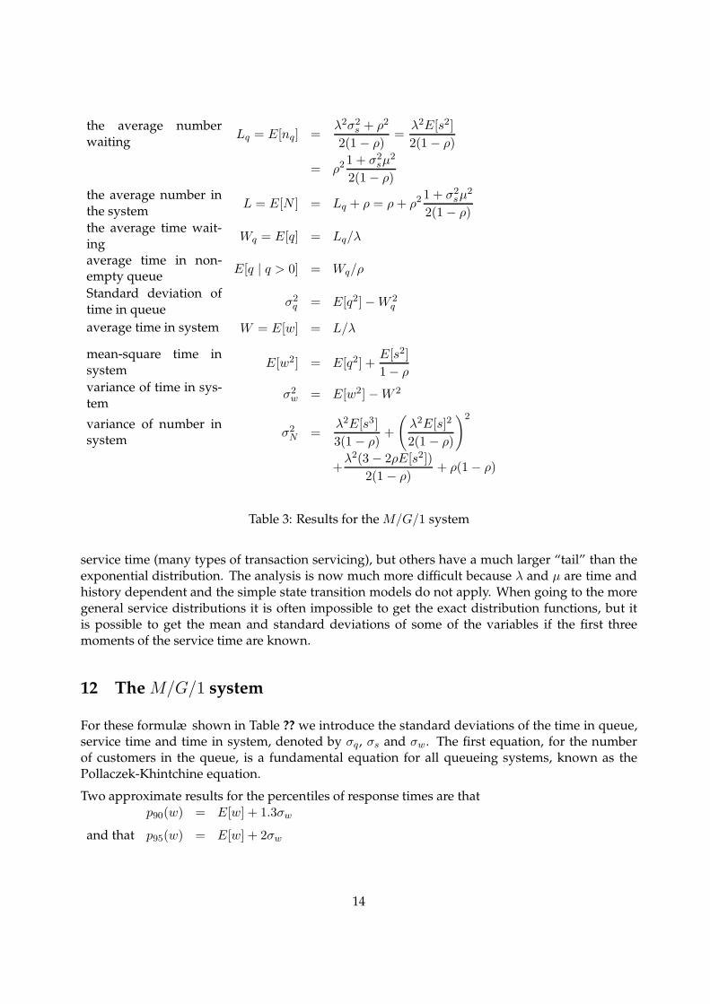
the average numberwaiting

Lq = E[nq] =λ2σ2

s + ρ2

2(1 − ρ)=

λ2E[s2]

2(1 − ρ)

= ρ2 1 + σ2sµ

2

2(1 − ρ)

the average number inthe system

L = E[N ] = Lq + ρ = ρ + ρ2 1 + σ2sµ

2

2(1 − ρ)the average time wait-ing

Wq = E[q] = Lq/λ

average time in non-empty queue

E[q | q > 0] = Wq/ρ

Standard deviation oftime in queue

σ2q = E[q2] − W 2

q

average time in system W = E[w] = L/λ

mean-square time insystem

E[w2] = E[q2] +E[s2]

1 − ρvariance of time in sys-tem

σ2w = E[w2] − W 2

variance of number insystem

σ2N =

λ2E[s3]

3(1 − ρ)+

(

λ2E[s]2

2(1 − ρ)

)2

+λ2(3 − 2ρE[s2])

2(1 − ρ)+ ρ(1 − ρ)

Table 3: Results for the M/G/1 system

service time (many types of transaction servicing), but others have a much larger “tail” than theexponential distribution. The analysis is now much more difficult because λ and µ are time andhistory dependent and the simple state transition models do not apply. When going to the moregeneral service distributions it is often impossible to get the exact distribution functions, but itis possible to get the mean and standard deviations of some of the variables if the first threemoments of the service time are known.

12 The M/G/1 system

For these formulæ shown in Table ?? we introduce the standard deviations of the time in queue,service time and time in system, denoted by σq, σs and σw. The first equation, for the numberof customers in the queue, is a fundamental equation for all queueing systems, known as thePollaczek-Khintchine equation.

Two approximate results for the percentiles of response times are thatp90(w) = E[w] + 1.3σw

and that p95(w) = E[w] + 2σw

14

13 The M/Ek/1 queueing system

An important case of the M/G/1 system is the M/Ek/1 system, for the Erlang-k service time dis-tribution (a cascade of exponential servers). The earlier equation is repeated, but now writing µinstead of λ, to emphasise that it describes a service distribution rather than an arrival distribu-tion. The average service rate is µ.

Ek(x) = 1 −k−1∑

j=0

(µx)j

j!e−µx

For large values of k, the Erlang-k distribution tends towards a rectangular distribution with acut-off of 2µ. The moments of the service time, for substitution into the Table ?? results for theM/G/1 system, are –

second moment E[s2] =(k + 1)

kµ2

third moment E[s3] =(k + 1)(k + 2)

k2µ3

14 The M/D/1 system

With a constant service time s, we use the M/G/1 model with σs = 0, E[s] = s, E[s2] = s2,E[s3] = s3, etc. The simplest important result is that the average number waiting is half thatwaiting with exponentially distributed service.

Lq =ρ2

2(1 − ρ)

the total number in the system N =ρ2

2(1 − ρ)+ ρ

the mean time in the system W =(2 − ρ)

2µ(1 − ρ)

std devn of number in system σN =1

1 − ρ

√

ρ −3ρ2

2+

5ρ3

6−

ρ4

12

Other results can be derived from the M/G/1 equations.

15 The Erlang B and Erlang C formulæ

A telephone exchange normally has a number of incoming lines, served by a number of switcheswhere any switch can service any one of a group of lines. (There are often about 1000 lines to agroup.) If at least one switch is free the call can be accepted immediately. If all switches are busythe result depends on the design of the exchange.

15

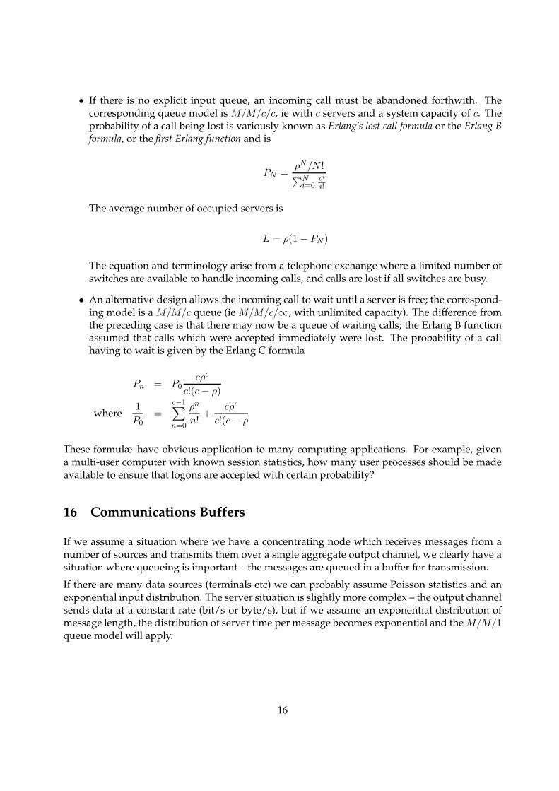
• If there is no explicit input queue, an incoming call must be abandoned forthwith. Thecorresponding queue model is M/M/c/c, ie with c servers and a system capacity of c. Theprobability of a call being lost is variously known as Erlang’s lost call formula or the Erlang Bformula, or the first Erlang function and is

PN =ρN/N !∑N

i=0ρi

i!

The average number of occupied servers is

L = ρ(1 − PN )

The equation and terminology arise from a telephone exchange where a limited number ofswitches are available to handle incoming calls, and calls are lost if all switches are busy.

• An alternative design allows the incoming call to wait until a server is free; the correspond-ing model is a M/M/c queue (ie M/M/c/∞, with unlimited capacity). The difference fromthe preceding case is that there may now be a queue of waiting calls; the Erlang B functionassumed that calls which were accepted immediately were lost. The probability of a callhaving to wait is given by the Erlang C formula

Pn = P0cρc

c!(c − ρ)

where1

P0=

c−1∑

n=0

ρn

n!+

cρc

c!(c − ρ

These formulæ have obvious application to many computing applications. For example, givena multi-user computer with known session statistics, how many user processes should be madeavailable to ensure that logons are accepted with certain probability?

16 Communications Buffers

If we assume a situation where we have a concentrating node which receives messages from anumber of sources and transmits them over a single aggregate output channel, we clearly have asituation where queueing is important – the messages are queued in a buffer for transmission.

If there are many data sources (terminals etc) we can probably assume Poisson statistics and anexponential input distribution. The server situation is slightly more complex – the output channelsends data at a constant rate (bit/s or byte/s), but if we assume an exponential distribution ofmessage length, the distribution of server time per message becomes exponential and the M/M/1queue model will apply.

16

The mean number in the system is N =ρ

1 − ρ

the average delay W =N

λ=

ρ

1 − ρ

1

λ

=1/µ

1 − ρ=

1

µ − λ

and the average queue length Lq =ρ2

1 − ρ

In many cases we have messages of constant length; the M/D/1 queue model is then applicable.If the message transmission time is µ, then the service time λ = 1/µ. Then,

the mean number in the system N =ρ

1 − ρ

(

1 −ρ

2

)

the mean time in the system W =1/µ

1 − ρ

(

1 −ρ

2

)

=1

µ − λ

(

1 −ρ

2

)

In both cases the change to constant service time yields the old result (M/M/1 queue) with themultiplier (1 − ρ/2), which is always less than 1.0. The difference is entirely due to the variationin service times with the M/M/1 queue discipline. There is little change at light loading, but asthe traffic intensity approaches 1, the delay for the M/D/1 queue tends to half the delay for theM/M/1 queue.

The number in queue and the delay (for µ = 1.00) are -

number & delayρ M/M/1 M/D/1

0.1 0.111 0.1060.2 0.250 0.2250.3 0.429 0.3640.4 0.667 0.5330.5 1.000 0.7500.6 1.500 1.0500.7 2.333 1.5170.8 4.000 2.4000.9 9.000 4.950

0.95 19.000 9.9750.99 99.000 49.995

The normal rule of thumb is that an M/M/1 queue becomes overloaded for (ρ > 0.6). The over-load point for fixed service time (M/D/1 queue) occurs at a rather higher traffic intensity, at aboutρ = 0.7. We can also calculate the number of buffers to ensure an upper limit of message rejectiondue to buffer overload.

17

16.1 Example 1

Assume that a multiplexer must accept 100 messages per second and that the user can tolerate aloss of no more than 10 messages in an 8-hour day. How many buffers must provided to guaranteethis service?

There are 100 × 3600 × 8 = 2, 880, 000 messages in a day, of which no more than 10 may be lost.The probability of all buffers being full may not exceed 10/2, 880, 000 = 3.5× 10−6. Given that theprobability of there being n customers in the system is ρn+1, we must have that

ρn+1 < 3.5 × 10−6

or (n + 1) loge ρ < −12.57n > −12.57/ loge ρ − 1

The table of n as a function of ρ, is

ρ Number ofbuffers

0.2 70.3 100.4 130.5 180.6 240.7 350.8 560.9 119

This is another argument for ensuring that a system is operating well within its apparent capacity.Not only do delays increase with loading, but so does the probability of buffer overflows. Ifthe multiplexer operates at only 50% of its nominal load, a pool of at least 20 buffers should beprovided to queue the input messages. (If the average message length is 100 bytes so that themultiplexer must handle 10,000 bytes per second, it should be rated at 20,000 bytes per second onits output line and have at least 20 message buffers.) Most actual multiplexers can invoke flowcontrol procedures to inhibit traffic as overload approaches, but this example indicates just howmuch buffering may be needed in high speed data logging with asynchronous inputs.

16.2 Example 2

An 8 channel multiplexer has a nominal capacity of 500 char/s and has an input buffer of 50characters for each channel. Each channel may tolerate no more than one lost character per day(8 hours). What is the maximum utilisation of the multiplexer?

Each channel has a nominal capacity of 1,800,000 characters in 8 hours, giving a permitted errorprobability of 0.556 × 10−6 and ρ51 < 0.556 × 10−6, whence ρ < 0.75. Increasing the buffer to 100characters allows ρ to reach 0.87.

18

17 Performance of Sequential access Networks

This analysis applies to all networks in which the right to transmit cycles in a regular manneramong the stations, including token ring and token bus. The machine repair model applies whencustomers need only occasional service and the service agent may be idle; this analysis is moreapplicable where queues exist at most stations and there is continuous traffic. It also shows an al-ternative approach to a queueing problem based on physical arguments as much as mathematicalones.

Consider a network of N nodes or stations, with an average walk time w for data (or control) topass from one node to its successor. Thus the time for control to pass around the entire networkis L = N.w, the system walk time. In some cases there may be different walk times for data transferand control transfer the choice is usually obvious.

A user who wishes to transmit sees an “access time” from submitting the packet until the packetis finally sent. It has two components

• the “walk time” as control circulates to the node, and

• the queueing time, behind preceding messages (this includes the transmission time)

The access time may be derived by a simple physical argument. The time for control to circulatearound the network, in the absence of any user traffic, is the walk time, L. A station which receivesa message and wishes to transmit must wait, on average, for half this time before receiving theright to transmit, or a time of L/2. If, however, the network is busy with a utilization ρ, the rightto transmit can circulate only when the network is idle; the circulation speed is reduced by thefactor (1 − ρ) and the system walk time then becomes

L

2

1

(1 − ρ)

For the queueing delay, note that there are potential queues at each node and that these queuesare served sequentially – the queue for the next node effectively continues on from the tail of thequeue for the current node, and so on. Thus there is really just a single circular queue whichis broken among the nodes and which needs transitions between nodes at appropriate times.However, messages which arrive at an arbitrary node will on average arrive at the mid-point ofthe effective queue and have half the usual waiting time.

19

����

A

����

B

����

C����

D

����

E

ZZ

ZZ

Z~

6

� �

?

Queue Bfollowsqueue A

�������

?

Queue Cfollowsqueue B

�

?��6Queue D follows queue C

CCCCCCO

6

Queue Efollowsqueue D

��

��

�>

6

� �?

Queue Afollowsqueue E

The queueing delay is then half that for a single queue. The normal waiting time in a queue is

Wq =ρ

1 − ρ

1

µ

For a sequential network with an arrival rate of λ per node (Nλ overall) the network utilisationis ρ = λNm, where m is the average message service time. For an exponential distribution ofmessage lengths, we have that m = 1/µ, giving

ρ =λN

µ

then Wq =Nλ

µ2(1 − ρ)

Thus E(D) =L

2

1

1 − ρ+

Nλ

2µ2(1 − ρ)

=n

2

1

(1 − ρ)

(

w +λ

µ2

)

Writing ρ in terms of λ and µ, the expected delay is

E(D) =Nµ

2(µ − Nλ)

(

w +λ

µ2

)

For packets of constant size, the queueing delay is halved and the ex-pected delay is

E(D) =Nµ

2(µ − Nλ)

(

w +λ

2µ2

)

20

The delay is therefore dependent on the difference of the arrival and service rates (equivalent tothe term 1/(1 − ρ) and on the relative values of the walk time between nodes (w) and the timebetween message arrivals (1/µ), weighted by the ratio of service time to arrival time. Given thatλ and µ are fixed by the desired user traffic and the network transmission speed, it is clear that wmust be as small as possible for good performance.

More exact models give slightly different results. For each station having a packet arrival rate λ,the same frame statistics (the second moment of frame length = m2 and the same walk time w,one model gives the average access delay as

E(D) =tc2

(

1 −ρ

N

)

+Nλm2

2(1 − ρ)

=L

2

(1 − ρ/N)

1 − ρ+

Nλm2

2(1 − ρ)

In these formulæ m2 is the second moment of the frame length and ρ = Nλm is the network util-isation. The first term is related to the circulation of the transmission right and for low utilisationis just half the system walk time. The numerator is related to the utilisation of each node, and thedenominator to the overall traffic intensity. The second term is in fact the average waiting timefor an M/G/1 queue.

Another analysis gives a similar result, but with (1+ρ/N) in the numerator. As the simple analysispresented here gives the average of these two “more exact” results, it seems to be just as good aseither of the “better” approaches.

As both terms are dominated by the factor 1/(1− ρ) we must minimise the system walk time L toensure performance at high utilizations. In most cases this means minimising the token latencyat each node. We will also see that the token ring is much better in this regard than the token bus,simply because of the token-passing overheads.

21