R & D Report 1993:7. Variance estimation in the Swedish consumer price index / Jorgen Dalén; Esbjörn Ohlsson. Digitaliserad av Statistiska centralbyrån (SCB) 2016. urn:nbn:se:scb-1993-X101OP9307

INLEDNING

TILL

R & D report : research, methods, development / Statistics Sweden. – Stockholm :

Statistiska centralbyrån, 1988-2004. – Nr. 1988:1-2004:2.

Häri ingår Abstracts : sammanfattningar av metodrapporter från SCB med egen

numrering.

Föregångare:

Metodinformation : preliminär rapport från Statistiska centralbyrån. – Stockholm :

Statistiska centralbyrån. – 1984-1986. – Nr 1984:1-1986:8.

U/ADB / Statistics Sweden. – Stockholm : Statistiska centralbyrån, 1986-1987. – Nr E24-

E26

R & D report : research, methods, development, U/STM / Statistics Sweden. – Stockholm :

Statistiska centralbyrån, 1987. – Nr 29-41.

Efterföljare:

Research and development : methodology reports from Statistics Sweden. – Stockholm :

Statistiska centralbyrån. – 2006-. – Nr 2006:1-.

Variance Estimation in the Swedish Consumer Price Index

Jörgen Dalén och Esbjörn Ohlsson

R&D Report Statistics Sweden

Research - Methods - Development 1993:7

Från trycket Oktober 1993 Producent Statistiska centralbyrån, utvecklingsavdelningen Ansvarig utgivare Lars Lyberg Förfrågningar Jörgen Dalen, tel 08-783 44 94

© 1993, Statistiska centralbyrån ISSN 0283-8680

Printed October 1993 Producer Statistics Sweden,

Department of Research and Development S-115 83 Stockholm

Publisher Lars Lyberg Inquiries Jörgen Dalen, telephone +46 08 783 44 94

© 1993, Statistics Sweden ISSN 0283-8680

VARIANCE ESTIMATION IN THE SWEDISH

CONSUMER PRICE INDEX

by

Jörgen Dalén, Department of Economic Statistics, Statistics Sweden Esbjörn Ohlsson, Mathematical Statistics, Stockholm University

Abstract: In large parts of the Swedish Consumer Price Index, products and outlets are sampled independently, yielding a two-dimensional, cross-classified sample. In this paper, a variance formula for this index is derived by exploiting the general theory for cross-classified sampling. Numerical variance estimates are given, along with a description of some of the detailed procedu­res involved in their computation. Finally, the implications of these estimates on the actual allocation is discussed.

Key words: Cross-classified sampling, two-dimensional sampling, sampling error.

Table of Contents 1. Introduction 1 2. The KPI sampling structure 1 3. Index definition and estimator 2 4. The variance of the index 5 5. Variance estimators 6 6. Variance estimation in practice 7

6.1 The List Price System (LIPS) 7 6.2 The Local Price System (LOPS) 7 6.3 Other price surveys 8

7. Numerical results for 1991 and 1992 9 8. The allocation problem 11 9. References 12 Appendix 1: Tables 14 Appendix 2: Derivation of the variance formula 17

1. Introduction

This report is concerned with estimating the sampling error of the Swedish Consumer Price Index (in Swedish "Konsumentprisindex", KPI for short). Large parts of the KPI are based on price quotations from two-dimensional samples, each of which is the cross-classification of a sample of outlets (shops, restaurants, etc.) and a sample of products (items, commodities). In the sequel, such a procedure for sampling from a two-dimensional population will be called Cross-Classified Sampling. Ohlsson (1992) gave general results on the variance of an estimator based on a cross-classified sample. In this report we will use these general results to derive estimators of the sam­pling variance of the KPI. Numerical results for 1991 and 1992 will also be given.

The problem of estimating the sampling variance of a CPI has received quite some interest during the last years. An early reference is Banerjee (1956), who addresses the problem of optimal allocation of the item sample. The first one to give numerical variance estimates for a CPI is, as far as we know, Wilkerson (1967). Recent papers include Leaver & Valliant (1993) on the United States CPI; the two-dimensional sample in the US is, however, a two-stage sample and not a CCS. Balk & Kersten (1986) and Biggeri & Giommi (1987) use balanced half-samples and similar methods to estimate the variance due to the use of weights from a household expenditure survey. Other important papers are Leaver et al (1991) and Leaver & Swanson (1992), which give numerical estimates of the variance for the US CPI for the years 1978-1986 and 1987-1991, respectively, conditional on the expenditure weights.

In Sweden Ruist (1953) and Malmquist (1958), both in Swedish, are early attempts to estimate the KPI sampling error. The (one-dimensional) variance due to the sampling of outlets in the KPI, conditioning on the item sample and making the simplifying assumption of with replacement sampling was computed by Andersson, Forsman & Wretman (1987).

If simple random sampling without replacement (srswor) is used in both dimensions, a variance formula can be obtained from Vos (1964). The connection between the KPI samples and Vos' theory was first noted by Dalen (1992). Since the outlet and product samples are typically drawn with probability proportional to size (pps), Vos' results cannot be applied to the KPI. The generalization to the pps case is given in Ohlsson (1992).

This paper starts by giving an overview of the KPI sampling system in Section 2 . In Section 3 the index definition and estimator are given and in Section 4 the theoretical variance formulas are presented. Section 5 gives the variance estimators and Section 6 discusses the actual procedures in applying these estimators to the actual KPI surveys. Section 7 presents and discusses numerical results for 1991-1992 and Section 8 deals with the problem of optimal allocation.

To the best of our knowledge, the present paper is the first to give numerical variance estimates based on a design-based variance formula for a CPI.

2. The KPI sampling structure

A distinctive feature of the Swedish KPI is that it is composed of many (50-60) independent price surveys for different product groups. Some of these are large in terms of the total weight covered but several are very small.

The all item KPI could be written as a sum of weighted one-survey indices:

(2.1)

1

where Ik is the one-survey index and wk the aggregate weight of all items in that survey. Based on sample data the Ik are estimated independently, by îk say, giving rise to the estimated KPI, I. Hence, the aggregate variance can be computed simply as

(2.2)

Hence, an overall variance estimator can be derived by estimating the V(Ik) for each survey separately.

The real problem is how to estimate variances for each individual survey. In the search for such estimates we have given priority to large surveys. For surveys covering about 45% of the weight, thorough variance estimates have been done. For surveys covering an additional 35% of the weight we have made less thorough estimates of the order of size of the variances. Based on general knowledge of the price data, the many independent, small surveys making up for the remaining 20% of the weight are not believed to influence a measure of total KPI sampling error significantly. Thorough variance estimates for these surveys are yet to be done.

There are two major sampling dimensions in a CPI for measuring price change - of outlets and of products. In many countries purposive sampling is used in one or both of these dimensions. As far as we know, the only country attempting an all out probability design for its CPI is the United States. In Sweden, outlet sampling is mainly done by probability. Product sampling is done by probability for product groups covering about 18% of the KPI weight while as purposive selection is used for about 40%. For other product groups there is either no product sampling at all (all products are covered) or the distinction between outlets and products is not clear. In the latter cases various mixtures of probability-based and purposive procedures are used.

There is also a third sampling dimension in a CPI - for the estimation of weights. In the KPI weights are mainly taken from the National Accounts that in its turn use retail trade surveys, household budget surveys and other sources. The weight dimension is not further discussed in this report. See Dalen (1993) for a discussion of this and other KPI errors.

The approach in this paper is basically design-based. From this point of view there is no such thing as a variance from a purposive sample. But there is an obvious need to compute some measure of the contribution to the KPI error, due to purposive sampling, at the very least for the purpose of obtaining a rational allocation with respect to the size of the outlet sample vs. the size of the pro­duct sample. Our approach on this issue is to calculate variances from purposive samples as if they were drawn by probability, with a design similar to the actual probability samples in some other parts of the KPI. This requires setting up a "dummy design" for the purposive selection reflecting as closely as possible how this selection was actually done. This approach corresponds to that of quasi-randomization when modelling the non-response distribution in surveys, see e.g. Särndal, Swensson and Wretman (1992, page 574). Below (in Section 6.2) we describe the construction of a postulated design in the largest KPI price survey.

With this approach we get a unified framework for estimating the variance of several important KPI surveys. An alternative would of course be to change to a model-based approach for the entire KPI. This alternative has not been investigated.

3. Index definition and estimator

The general theory of variance calculation in cross-classified sampling (CCS) is given in Ohlsson (1992). In CCS there are two independent sampling dimensions, rows and columns. In each dimension the samples may be stratified and/or drawn with unequal inclusion probabilities.

2

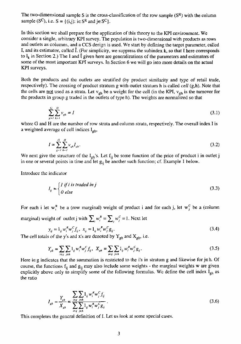
The two-dimensional sample S is the cross-classification of the row sample (SR) with the column sample (Sc), i.e. S = {(i,j): ieSR and j e S c } .

In this section we shall prepare for the application of this theory to the KPI environment. We consider a single, arbitrary KPI survey. The population is two-dimensional with products as rows and outlets as columns, and a CCS design is used. We start by defining the target parameter, called I, and its estimator, called Î. (For simplicity, we suppress the subindex k, so that I here corresponds to Ik in Section 2.) The I and Î given here are generalizations of the parameters and estimators of some of the most important KPI surveys. In Section 6 we will go into more details on the actual KPI surveys.

Both the products and the outlets are stratified (by product similarity and type of retail trade, respectively). The crossing of product stratum g with outlet stratum h is called cell (g,h). Note that the cells are not used as a strata. Let vgh be a weight for the cell (in the KPI, vgh is the turnover for the products in group g traded in the outlets of type h). The weights are normalized so that

(3.1)

where G and H are the number of row strata and column strata, respectively. The overall index I is a weighted average of cell indices Igh,

(3.2)

We next give the structure of the I„h's. Let fy be some function of the price of product i in outlet j in one or several points in time and let gy be another such function; cf. Example 1 below.

Introduce the indicator

(3.3)

For each i let wjr be a (row marginal) weight of product i and for each j , let w^ be a (column

marginal) weight of outlet j with ^ , . vv,R = ^T wyc = 1. Next let

(3.4) The cell totals of the y's and x's are denoted by Ygh and Xgh, i.e.

(3.5)

Here ie g indicates that the summation is restricted to the i's in stratum g and likewise for je h. Of course, the functions fy and gy may also include some weights - the marginal weights w are given explicitly above only to simplify some of the following formulas. We define the cell index Igh as the ratio

(3.6)

This completes the general definition of I. Let us look at some special cases.

3

Example 1. Suppose the index is a measure of change in the price level from time 0 to time 1. Let

py be the price of i in j at time t; t=0,l. Upon putting fy = py and gy = p°, Igh becomes a ratio of

(weighted) mean prices. If instead we let fy = py / p° and gy = 1, then Igh becomes a (weighted)

mean of price ratios. In the KPI we put

(3.7)

and the weights wf and Wjare (rough) measures of turnover of the product and outlet,

respectively. See Dalen (1992) for the reasons for using (3.7).

We conclude that, by proper choice of fy and gy, we can make (3.6) cover many common index formulas, with a notable exception for the geometric mean of price ratios. •

We now turn to the definition of the estimator I of the index defined above. We shall assume that the indicators ly and the prices (and hence fy and gy) are known only for the sample, while the

weights wf and w^ are known for the entire population. This corresponds to the actual KPI

situation. In product stratum g, the sample Sr is assumed to be drawn with probabilities

proportional to the wf, i.e., for some predetermined sample size mg

(3.8)

In outlet stratum h, the sample S^ is assumed to be drawn with probabilities

(3.9)

for some sample size nh. Here we must assume that the quantities on the right-hand side of (3.8) and (3.9) do not exceed 1. In practice this is achieved by, whenever necessary, forming separate complete enumeration strata for large units. Taking care of such strata is a straight-forward task, but it makes the formulas rather involved. For simplicity we will, in the theoretical exposition, assume that no large unit strata are necessary.

The Horvitz-Thompson estimator of Ygh and Xgh are, by (3.5), (3.8) and (3.9).

(3.10)

respectively. As an estimator of the ratio in (3.6) we take

(3.11)

Note that îgh is "self-weighting"; this property is lost by the introduction of large unit strata, though. Finally the estimated I is, by (3.2),

(3.12)

4

4. The variance of the index

We shall apply the general CCS theory to find an expression for the variance V(î). In doing so we must specify the sampling procedures that are used to generate samples with inclusion probabilities as in (3.8) and (3.9). The actual sampling procedures used in the surveys of interest are: sequential Poisson sampling (of outlets), random systematic PPS sampling (of products in one system) and purposive sampling (of products in one system). For a description of random systematic sampling and ordinary Poisson sampling, see e.g. Brewer & Hanif (1983, p.22); for a description of sequential Poisson sampling see Ohlsson (1990 and 1993). For simplicity, we will postulate random systematic PPS sampling in both dimensions, cf. the discussion on purposive sampling in Section 2.

As usual when estimating a ratio, I is not unbiased. As argued in Appendix 2, Î is approximately unbiased, though. Hence, we measure the sampling error by V(î), as an approximation to the mean square error of Î. The simulation studies in Section 7 of Ohlsson (1992) indicate that the bias is indeed small as compared to the variance.

Before presenting the formula for V(î), we introduce some further notation. For i€g and je h, let

(4.1)

and put

(4.2)

Proposition 4.1: The variance of the index I can be approximated as follows

(4.3)

(4.4)

(4.5)

(4.6)

The derivation of this proposition from the general results in Ohlsson (1992) is postponed to Appendix 2.

The approximation in (4.3) is partly due to the use of a standard type linearization of the ratio estimator, (see Appendix 2, formula A.l). and partly due to the use of approximations for the second order inclusion probabilities of random systematic sampling, (see Appendix 2, formula A.8). VPRO will be called the "variance between products", VOUT the "variance between outlets",

5

while VINT is "outlet and product interaction". A reason for this terminology is that VPRO is the variance that would result if outlets were completely enumerated, and similarly for VOUT. (This fact can not be seen in the above formulas, because of their approximative nature, but it is easily seen in the exact variance formulas in Ohlsson, 1992).

TheVINT component does not have the interaction structure one might expect from Ohlsson (1992, formula 1.9) and the fact that srswor is a particular case of random systematic sampling. Presumably this is caused by the approximation of the second order inclusion probabilities (A.8).

Suppose, however, that the finite population corrections l - (m s — l)wr and 1-(«A-l)wyc are all

close to 1, and hence can be omitted. Then it is readily seen that VINT can be rewritten as

(4.7)

(4.8)

egh1 is inserted into (4.7) only to reveal the similarities with the interaction term in a two-way analysis of variance table; cf. also Ohlsson (1992, formula 1.9).

5. Variance estimators

In deriving the variance estimators presented below we will basically use Proposition 4.1 which is valid for random systematic sampling. Piecewise Horvitz-Thompson estimation is used for unknown population quantities. The finite population corrections (fpc) are, however, adjusted on heuristic grounds so that they become zero for sampling units included with probability one. This can also be viewed as a "calibration to srswor", meaning that the fpc's have been adjusted so that the variance formulas are exact in case all selection probabilities are equal. In such a case, random systematic sampling reduces to srswor; hence we would like our variance formulas to be identical to the ones for srswor. The fact that this is not the case before adjustment can be attributed to the approximation of the second-order inclusion probabilities in (A.8) which is used to derive Proposition 4.1. The adjustment is important in cases of inclusion probabilities equal (or close) to one where we want the fpc's to be equal (or close) to zero.

Similarly, the variance estimators were inflated by factors mg/(mg-l) and nh/(nh-l) to "calibrate" to the unbiased variance estimator in srswor.

When trying to estimate (4.6) we ended up with negative variance estimates in certain cells. The reason is presumably that the approximation procedure in (A.8) does not work well in this situation. We therefore turned to a quadratic structure of the V1NT component as in (4.7). Fortunately, as we shall see, the contribution of VINT to V(î) is much smaller than that of VPR0

and VO U T.

The following formulas were thus used for variance estimation:

(5.1)

(5.2)

6

(5.3)

èf is as in (4.1) but with î h replacing I h„

(5.4)

6. Variance estimation in practice

The variance estimation procedures above were applied to two of the major price measurement systems in the KPI. These are the List Price System (LIPS) and the Local Price System (LOPS).

6.1 The List Price System (LIPS)

In LIPS probability sampling is used for products as well as outlets. Prices are taken from wholesalers' price lists for each month except December when interviewers collect actual prices in the shops. (From 1993 price lists are no longer be used at all.) LIPS accounts for about 18% of the total CPI weight.

LIPS covers most food products (not fresh food such as fruits and vegetables, bread and pastries or fish) and other daily commodities such as those typically found in a supermarket. Sampling of products is based on historic sales data from the three major wholesalers in Sweden using systematic PPS sampling of products, stratified into about 60 product strata.

Sampling of outlets is done by pps sampling, viz. sequential Poisson sampling (Ohlsson, 1990 and 1993). The size measure is number of employees plus 1, used as a rough measure of turnover. The outlets are first stratified by region and (to a certain extent) wholesaler. The product sample is matched to the sampled outlets so that the outlet is given the product sample of the wholesaler that delivers its goods.

There were about 1200 products in the sample in 1991-1992. The number of outlets was 58 in 1991 and 59 in 1992.

Our postulated design (which is a slight simplification of the actual one) uses an asymmetric stratification structure. We start by stratifying the whole product-outlet population into three wholesaler strata. In each of these primary strata cross-classified sampling is done independently. In each primary stratum an unstratified PPS sample of outlets is cross-classified with a stratified PPS sample of products. This gives the following variance structure

(6.1)

where the wh are market share weights of the three wholesalers and the Vh(I) are variances in primary strata which in turn have three components computed as in (5.1)-(5.3). Note that there is now only one outlet stratum within each primary stratum.

6.2 The Local Price System (LOPS)

In LOPS interviewers collect prices each month. The system accounts for about 21% of the total CPI weight.

7

Outlets are divided into 25 strata according to the SNI code (Swedish Code of Industrial Classification which closely follows the International Standard of Industrial Classication - ISIC) of the outlet. Within a stratum sequential Poisson sampling is used as in LIPS.

For products, however, purposive sampling is used in several steps. The products are divided into product groups according to the National Accounts and other sources of information . Within a product group one or more products are chosen, often only one. All in all there are some 140 "representative products" in LOPS. For each of these 140 products a commodity specification is done at the central office. The interviewer is then asked to find the particular variety according to the specification that is the most sold within the surveyed outlet.

The actual sampling procedure in LOPS is thus CCS with probability sampling of outlets, but purposive sampling of products. Our postulated design is, however, probability sampling of products, too.

There are 20 (1991) or 21 (1992) outlet strata (some strata are collapsed) and 48 (1991) or 43 (1992) product strata.

The forming of the product strata was based on the actual procedures used in the selection of the representative products. There the starting point is often information on the consumption value of a rather narrow product group like "bananas", "dish washers", or "towels". The final sample is then one or several representative products in each group. In our variance estimation procedures we consider these final products as randomly chosen from their respective product groups. For imputing a subjective "inclusion probability" into the variance formulas we basically ask the question. How much of the consumption value in this product group is accounted for by the product finally selected by the interviewer? For example for the product group bananas there is typically only one brand and one price in an outlet and we therefore set the inclusion probability to one for the representative product one kg of bananas within the product group bananas. On the contrary, a particular brand of the representative product towel, terry cloth, 100% cotton, hemmed, about 50x70 cm within the product group towels is likely to have a rather small share of an outlet's total sales value of towels and in this and many similar cases we set the "inclusion probability" to 0.1.

We believe that, although there are subjective elements in our procedure, it gives a fairly realistic picture of the random error arising from product sampling. The greatest problem is probably our procedures for collapsing product strata in those cases where only one product was selected in a product group. This may lead to some overestimation since products in the actual products strata could be expected to have more similar price movements than those in the collapsed strata.

6.3 Other price surveys

Variance computations were done for other price surveys too. The methods used were cruder and more simplified. The exact procedures are not of general interest so a short summary will be sufficient.

The apparel survey (covering about 6% of the total KPI weight) uses sequential sampling of outlets and a purposive sample of 24 garments. But in each outlet several (up to 8) varieties of each garment were priced. According to various comparability criteria only a certain portion of the varieties are included in the index. Here we used a simple one-dimensional variance estimation procedure based on the effective sample size for each garment.

8

The rental survey (directly 10% and with imputation about 13.5% of the weight) is based on a random sample of about 1000 apartments and is thus one-dimensional. The estimator is post-stratified into different size groups crossed with newly built versus old ones. The estimated index is a kind of unit-value index comparing the average rent per m2 for all apartments at two points of time, with corrections for differences in quality (equipment etc.) Here, our variance computations are simplified in so far that they do not take account of the changing population.

The interest survey (8.5% of the weight) estimates the amount of interest paid or foregone for owner-occupied homes by multiplying their total capital investment (defined as total purchase values) with the average interest rate. For estimating capital investment a stratified sample of some 650 homes was drawn in 1973. To this sample annual supplementary samples of newly built homes are added which gives a total sample of about 800 homes in 1992. Conditional variance calculations reflecting only the sampling for and estimation of capital investment have been done. This variance component is judged to dominate the sampling error of the interest survey.

The car survey (3%) was, in 1991, based on 31 brands of cars (60 in 1992). The design could be interpreted as stratified with one purposively selected unit in each stratum. Variances have been computed based on a crude assumption of simple random sampling. There is some evidence that this is a fairly reasonable assumption in this case.

The petrol survey (4%) covers five types of petrol (almost all existing) at 120 petrol stations, sampled with sequential Poisson sampling so variance estimation was done in a straight-forward way.

The survey of alcoholic beverages (2.6%) relies on information from the Swedish state monopoly for its total sales. It thus has zero sampling error (leaving aside taxfree sales at airports etc.).

Other product groups also have zero or very small sampling error. This is the case for, e.g., gambling and lotteries, TV license fees, hospital care and dental care (2.9% together).

For other surveys weights are so small that they could not influence a measure of total KPI sampling error significantly. Direct variance estimates have not yet been done, however.

7. Numerical results for 1991 and 1992

Up to now we have computed sampling errors for two years for the major price surveys. In Table 1-3 in Appendix 1 we give December-to-month variance estimates (within an annual link) for those surveys obtained with formulas (5.1)-(5.3) for the two largest surveys. In table 4-5 in Appendix 1 some other variance estimates are given.

The interpretation of these results is the following with LIPS as our example. VT 0 T for June 1991 is 0.0904. If the LIPS part of KPI for June 1991 with December 1990 as reference period were 104 an appropriate 95% confidence interval for its sampling error would be 104±1.96xV0.0904=104± 0.6. If LIPS had been the only source of sampling error in the KPI and the KPI figure for June 1991 was 105 then a 95% confidence interval for it would be 105±1.96xVo.00283=105±0.1. The contribution to the KPI variance is calculated according to (2.2) remembering that the weight for the whole LIPS system was 0.177 in 1991.

In LIPS only minor changes in the samples were done between 1991 and 1992. Still there were quite significant changes in the estimated variances. In early 1991, as well as for earlier years for which we have cruder estimates (not presented here), the VP R 0 and V0UT components are about the same size although, as mentioned in 3.1 above, there are 20 times more products than outlets. This means that the underlying between-product variation was much larger than the underlying

9

between-outlet variation and was the basic reason for the seemingly extreme allocation of the sample. We also note that the VINT component is of a much smaller order of size than VPRO and VOUT. In 1992 and particularly its last months, however, this relation changed with VPR0

decreasing and VOUT increasing. A possible explanation of this is that some outlets have changed their pricing behaviour, moving from quickly changing campaign prices to more stable "always-low-prices". It remains to be seen if this tendency will remain, in which case the allocation should be adjusted.

For LOPS (table 2) the VPRO component is always larger than VOUT. We have here some 800 outlets and 140 products. Since it costs less to include one more product than one more outlet in the sample, this means that we have had a poor allocation. These results have generated a successive movement towards a more efficient allocation with more products and fewer outlets in this survey which is the most expensive in the KPI, cf. Section 8.

The Apparel survey (table 3) shows increasing variances from 1991 to 1992 and is now the greatest concern in our KPI sampling design. Unfortunately, we have not so far been able to produce a good decomposition of this variance. A major problem here is that our criteria for comparability are sometimes so restrictive that the result is a very small effective sample. But more liberal comparability criteria lead to a risk for increasing biases instead. For 1993, measures have been taken to increase the efficiency of the comparability criteria.

For all these three surveys there is a tendency for the variances to increase over the year. This is of course to be expected since we measure changes from December and changes are generally small in the beginning of the year. In LOPS and the Apparel Survey, but not in LIPS, variances are also high during the summer. A feature which all three surveys have in common is the high variability of the variance estimates which complicates allocation decisions.

The Interest survey gave the conditional variance estimates for 1990-1992 presented in table 4.

For other price surveys than those discussed in some detail above, some crude estimates are given in table 5 only to show that their contributions to KPI variance is of a smaller order of size than for those surveys where we have used more careful procedures.

10

8. The allocation problem

In order to give a survey an optimal sampling allocation two things are neccessary: a variance function and a cost function. Above we have concentrated on the variance function. Here the cost function is first discussed .

In the Swedish KPI practice there are two levels of the allocation problem - between surveys and within surveys. So far we have not been able to give direct cost estimates to different surveys. As proxies we could use sample sizes which gives the following picture, with reference to 1991, for the surveys discussed above.

TABLE 6

Now, of course, costs are not generally proportional to sample size. In LIPS, for example, a mode of data collection (mainly price lists) was used which makes it much less expensive than LOPS (where interviewers to a large extent visit the outlets for price measurement) despite its larger sample size.

Some obvious misallocation is readily seen from table 5, however. The sample sizes of the car and the petrol survey should rather be reversed, for example. Also there is an obvious need for increasing the sample sizes for homes (for which the large variance was discovered only recently) and for apparel items.

When it comes to allocation within surveys, we take our most expensive survey, LOPS, as our example. Here we use the following cost function:

(8.1)

where C0 is a fixed cost for administration etc., nh is the number of outlets in outlet stratum h, mg is the number of items in item stratum g, a,, is the fixed cost per outlet in stratum h, mainly due to travel time, bh is the cost of measuring one item in outlets of stratum h and

11

rghk is the relative frequency of item ke g in outlets of stratum h.

In practice ah depends on the extent to which telephone interviews could be used for price measurement in stratum h. This could be done in most months, if there are few and simply defined items in the outlet.

The bh are the same for most strata but food items are generally simpler to measure and so bh is smaller for the daily commodity stores.

Now if we try to combine (8.1) with (5.1)-(5.3) we run into a non-linear optimization problem for which it seems impossible to find an explicit solution. A direction to go would therefore be to try some kind of numerical optimization procedure. So far we have not made attempts in this direction since the necessary work could be expected to be large.

Although a formal optimization has not been done, the variance and cost functions have made sizeable improvements in the LOPS allocation possible by simple inspection of the numerical results combined with calculation of marginal changes. We have increased the number of products (in particular in the highly variable product group fresh fruit and vegetables) in the survey while cutting down on the number of outlets. All together this has led to lower costs and smaller variance at the same time!

9. References

Andersson, C, Forsman, G. & Wretman, J. (1987). On the measurement of errors in the Swedish Consumer Price Index. Bull. Int. Stat. Inst. 52, Book 3, 155-171.

Balk, B.M. & Kersten, H.M.P. (1986). On the precision of Consumer Price Indices caused by the sampling variability of budget surveys. Journal of Economic & Social Measurement 14, 19-35.

Banerjee, K.S. (1956). A note on the optimal allocation of consumption items in the construction of a cost of living index. Econometrica 24, 294-295.

Biggeri, L. & Giommi, A. (1987). On the accuracy and precision of the Consumer Price Indices. Methods and applications to evaluate the influence of the sampling of households. Bulletin of the International Statistical Institute 52, Book 3, 137-154.

Brewer, K.R.W. & Hanif, M. (1983). Sampling with unequal probabilities. Springer, New York.

Connor, W.S. (1966). An exact formula for the probability that two specified sample units will occur in a sample drawn with unequal probabilities and without replacement. J. Amer Statist. Assoc.61, 384-390.

Dalen, J. (1992). Computing elementary aggregates in the Swedish Consumer Price Index, Journal of Official Statistics 8, 129-147.

Dalén, J. (1993). Quantifying errors in the Swedish Consumer Price Index. R&D Reports, Statistics Sweden.

Hartley, H.O. & Rao, J.N.K. (1962). Sampling with unequal probabilities and wihout replacement. Ann. Math. Statist.33, 350-374.

12

Leaver, S., Johnstone, J., & Archer, K. (1991). Estimating unconditional variances for the U.S. Consumer Price Index for 1978-1986. American Statistical Association, Proceedings of the Section on Survey Research Methods, 614-619.

Leaver, S. & Swanson, D. (1992). Estimating variances for the U.S. Consumer Price Index for 1987-1991. American Statistical Association, Proceedings of the Section on Survey Research Methods, forthcoming.

Leaver, S. & Valliant, R. (1993). Statistical problems in estimating the U.S. Consumer Price Index. To appear in Survey Methods for Businesses, Farms and Institutions. Wiley, New York.

Malmquist, S. (1958): Precisionsproblemet vid beräkning av konsumentprisindex, Statistisk Tidskrift 7, 492-504 and 612-628.

Ohlsson, E. (1990): Sequential Poisson sampling from a Business register and its application to the Swedish Consumer Price Index. R&D Report 1990:6, Statistics Sweden.

Ohlsson, E. (1992). Cross-classified sampling for the Consumer Price Index. R&D Report 1992:7, Statistics Sweden.

Ohlsson, E. (1993). Coordination of several samples using permanent random numbers. To appear in Survey Methods for Businesses, Farms and Institutions. Wiley, New York.

Ruist, E. (1953). Några synpunkter på socialstyrelsens prismaterial. In SOU 1953:23 Konsumentprisindex, Stockholm.

Särndal, C.E., Swensson, B., and Wretman, J. (1992). Model assisted Survey Sampling. Springer Series in Statistics.

Vos, J.W.E. (1964). Sampling in space and time. International Statistical Review 32, 226-241.

Wilkerson, M. (1967). Sampling error in the Consumer Price Index. Journal of the American Statistical Association 62, 899-914

13

Appendix 1: Tables

TABLE 1: Variance estimates in LIPS 1991-1992

14

TABLE 2: Variance estimates in LOPS 1991-1992

15

TABLE 3 Variance estimates in the Apparel Survey 1991-1992

TABLE 4 Conditional variance estimates in the interest survey

TABLE 5 Crude variance estimates for some price surveys

16

Appendix 2: Derivation of the variance formula

In this appendix we shall derive Proposition 4.1 from Theorem 2.1 and Theorem 3.1 in Ohlsson (1992).

Recalling (3.2), (3.6) and (3.11)-(3.12), we have the following (Taylor series) linear approximation.

(A.1) K" K"

From the unbiasedness of the Horvitz-Thompson estimator and (A.l) we conclude that Î is approximately unbiased. We can now concentrate on deriving the variance of the right-hand side of (A.l). Set

(A.2)

and note that by (3.5) and (3.6) the cell total Zgh is

(A.3)

Let ZKh be the Horvitz-Thompson estimator of Zgh. By (3.8), (3.9) and (4.1) we have

(A.4)

Let Z be the sum of ZKh over all cells. From (A.l) and (3.10) we get

(A.5)

We shall apply the results in Ohlsson (1992) to the right-hand side of (A.5). From Theorem 2.1 there we get a decomposition of V(Z) into three parts. We shall show, one by one, that these parts equal the three components in Proposition 4.1. We start with V P R O . In accordande with the mentioned theorem we first take the expectation over the outlet sample, conditional on the product sample, in (A.4) and get

(A.6)

Let Z be the sum of (A.6) over all column cells h, i.e.

(A.7)

According to Theorem 2.1 in Ohlsson (1922), the first component in V(Z) is V\£ Zg). Next note

that Z, is the (one-dimensional) Horvitz-Thompson estimator of the total ZK = ^ Zgh in case the

outlets are completely enumerated. Further note that the Z are independent, since they are based

on different strata. Recalling the well-known approximation formula for the variance of the Horvitz-Thompson estimator in random systematic sampling (formula 1.8.4 in Brewer & Hanif,

1983), we see that v ( ^ , Z Ä J is equal to the expression for VP R 0 in Proposition 4.1.

17

The expression for VQUT m the proposition is obtained from VPRO by noting the symmetry of rows

and columns in a CCS design. Our final concern is the interaction term VJJ^. According to Theorem 2.1 this term (called VRC there) can be found by adding all the within cells interaction terms. We therefore concentrate on a single cell and drop the cell indices g and h in the rest of the proof.

We shall apply Theorem 3.1 in Ohlsson (1992), which gives VINT in terms of inclusion probabilities. Connor (1966) supplied exact expressions for the second order inclusion probabilities in pps random systematic sampling. These expressions are unmanageable in practice, though. Instead, we shall use an approximation due to Hartley & Rao (1962), see also Brewer & Hanif (1983, p. 14). Omitting all th terms except the first one in this approximation we get

(A.8)

By inserting (A.8) into the expression for V]NT (VRC) given in Theorem 3.1, and using the fact that Z=0, we find

(A.9)

J J

By inserting (3.8), (3.9) and (A.2) into (A.9) we get (4.6) which completes the proof of Proposition 4.1.

18