R and the Bioconductor project

Sandrine Dudoit and Robert Gentleman

Bioconductor short course

Summer 2002

© Copyright 2002, all rights reserved

Everywhere …

• for statistical design and analysis: – pre-processing, estimation, testing, clustering,

prediction, etc.

• for integration with biological information resources (in house and external databases)– gene annotation (GenBank, LocusLink);– literature (PubMed);– graphical (pathways, chromosome maps).

Statistical computing

Outline

• Introduction to R and Bioconductor.• R programming

– environments and closures;– object oriented programming.

• Overview of Bioconductor packages– Biobase– genefilter– Annotate.

• Dynamic statistical reports using Sweave.

R

• R is a widely used open source implementation of the S language.

• S-PLUS is a commercial implementation of the S language.

• There are some differences between these two implementations but most books and papers describing one can be used for the other.

R resources

• R is available from www.r-project.org.• R is available for Unix, Windows, and

Macintosh computers.• A large number of software packages for

R are available from CRAN, www.cran.r-project.org.• These packages can easily be

downloaded and installed in your local computer.

Using R

• We presume some proficiency using R.

• There are a number of manuals, tutorials, and other resources available from the CRAN site if you feel that you need help.

• R also has detailed on-line documentation, in text, HTML, PDF, and LaTeX formats.

• help(name) • ? name

Bioconductor

• Bioconductor is an open source project to design and deliver high quality software and documentation for bioinformatics.

• Most of the early developments are in the form of R packages.

• Software and documentation are available from www.bioconductor.org.

Bioconductor

• Object-oriented class/method design. Allows efficient representation and manipulation of large and complex biological datasets of multiple types.

• Widgets. Specific, small scale, interactive components providing graphically driven analyses - point & click interface.

Bioconductor

• Interactive tools for linking experimental results to annotation and literature WWW resources in real time. E.g. PubMed, GenBank, LocusLink.

• Scenario. For a list of differentially expressed genes obtained from multtest or genefilter, use the annotate package to retrieve PubMed abstracts for these genes and to generate an HTML report with links to LocusLink for each gene.

Bioconductor packages

• General infrastructure– Biobase– annotate, AnnBuilder– tkWidgets.

• Pre-processing for Affymetrix data– affy.

• Pre-processing for cDNA data– marrayClasses, marrayInput, marrayNorm, marrayPlots.

• Differential expression– edd, genefilter, multtest, ROC.

• etc.

Bioconductor training

• Extensive documentation and training materials for self-instruction and short courses

– all available on WWW. • R help system

– interactive with browser or printable manuals;– detailed description of functions and examples;– e.g. help(genefilter), ?pubmed.

• R demo system – user-friendly interface for running demonstrations of R

scripts;– e.g. demo(marrayPlots).

Bioconductor training

• R vignettes system– comprehensive repository of step-by-step tutorials covering a

wide variety of computational objectives in /doc subdirectory;– use Sweave function from tools package.– integrated statistical documents intermixing text, code, and code

output (textual and graphical);– documents can be automatically updated if either data or

analyses are changed.

• Modular training segments – short courses: lectures and computer labs;– interactive learning and experimentation with the software

platform and statistical methodology.

R programming

• In order to deliver high quality software the Bioconductor project relies on a few programming techniques that might not be familiar: – enviroments and closures;– object oriented programming.

• We review these here for interested programmers (understanding them is not essential but is often very helpful).

Environments and closures

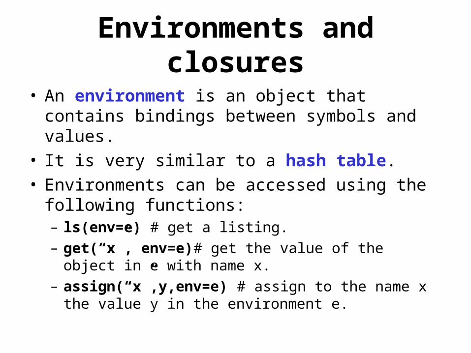
• An environment is an object that contains bindings between symbols and values.

• It is very similar to a hash table.• Environments can be accessed using the

following functions:– ls(env=e) # get a listing.– get(“x”, env=e) # get the value of the

object in e with name x.– assign(“x”,y,env=e) # assign to the name x the

value y in the environment e.

• Since these operations are used a great deal in Bioconductor we have provided two helper functions– multiget– multiassign

• These functions get and assign multiple values into the specified environment.

Environments and closures

• Environments can be associated with functions.• When an environment is associated with a

function, then that environment is used to obtain values for any unbound variables.

• The term closure refers to the coupling of the function body with the enclosing environment.

• The annotate, genefilter, and other packages take advantage of environments and closures.

Environments and closures

x <- 4

e1 <- new.env() assign(“x”,10, env=e1)f <- function() xenvironment(f) <- e1

x # returns 4f() # returns 10!

Environments and closures

Object oriented programming

• The Bioconductor project has adopted the OOP paradigm presented in Programming with Data, J. M. Chambers, 1998.

• Tools for programming using the class/method mechanism are provided in the methods package.

OOP

• A class provides a software abstraction of a real world object. It reflects how we think of certain objects and what information these objects should contain.

• A class defines the structure, inheritance, and initialization of objects.

• Classes are defined in terms of slots which contain the relevant data.

• An object is an instance of a class.

OOP• A method is a function that performs an

action on data (objects).

• A generic function is a dispatcher, it examines its arguments and determines the appropriate method to invoke.

• Examples of generic functions include plot, summary, print

OOP

• It is important to realize that when calling a generic function (such as plot) the actions performed depend on the class of the arguments.

• Methods define how a particular function should behave depending on the class of its arguments.

• Methods allow computations to be adapted to particular data types, i.e., classes.

OOP

• To obtain documentation (on-line help) about – a class: class?classname

so, class?exprSet, will display the help file for the exprSet class.

– a method: methods?methodname

so, methods?print, will display the help file for the print methods.

OOP

> x <- 1:10> y <- 2*x + 1 + rnorm(10)> class(x)[1] "integer"> plot(x,y)> fit <- lm(y ~ x)> class(fit)[1] "lm"> plot(fit)

OOP

• The methods package contains a number of functions for defining new classes and methods (e.g. setClass, setMethod) and for working with these classes and methods.

• A tutorial is available at http://www.omegahat.org/RSMethods/index.html

OOP

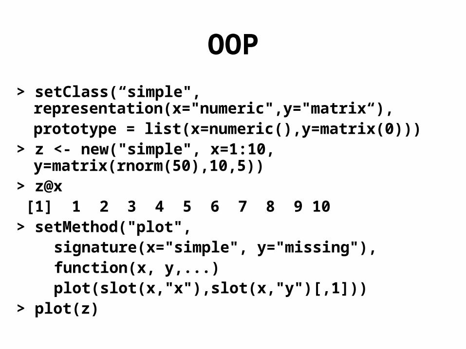
> setClass(“simple", representation(x="numeric",y="matrix“),

prototype = list(x=numeric(),y=matrix(0)))

> z <- new("simple", x=1:10, y=matrix(rnorm(50),10,5))

> z@x [1] 1 2 3 4 5 6 7 8 9 10> setMethod("plot",

signature(x="simple", y="missing"), function(x, y,...)

plot(slot(x,"x"),slot(x,"y")[,1]))> plot(z)

Biobase

• The Biobase package provides class definitions and other infrastructure tools that will be used by other packages.

• The two important classes defined in Biobase are– phenoData: sample level covariate data.– exprSet: the sample level covariate data

combined with the expression data and a few other quantities of interest.

Biobase: exprSet

Slots for the exprSet class• exprs: a matrix of expression measures, genes

are rows, samples are columns.• se.exprs: standard errors for the expression

measures, if available.• phenoData: an object of class phenoData that

describes the samples.• annotation: a character vector.• description: a character vector.• notes: a character vector.

Biobase: exprSet

description

annotation

phenoData

Any notes

Matrix of expression measures, genes x samples

Matrix of SEs for expression measures

Sample level covariates, instance of class phenoData

Name of annotation data

Covariate labels

se.exprs

exprs

notes

Biobase: exprSet

• One of the most important tasks is to align the expression data and the phenotypic data (and to keep that alignment through the analysis).

• To achieve this, the exprSet class combines these two data sources into one object, and provides subsetting and access methods that make it easy to manipulate the data while ensuring that they are correctly aligned.

Biobase: exprSet

• A design principle that was adopted for the exprSet and other classes was that they should be closed under the subset operation.

• So any subsetting, either of rows or columns, will return a valid exprSet object.

• This makes it easier to use exprSet in other software packages

Biobase: exprSet

Some methods for the exprSet class• show: controls the printing (you seldom want

a few hundred thousand numbers rolling by).• subset, [ and $, are both designed to keep

correct subsets of the exprs, se.exprs, and phenoData objects.

• split, splits the exprSet into two or more parts depending on the vector used for splitting.

Biobase: exprSet

• geneNames, retrieves the gene names (row names of exprs).

• phenoData, pData, and sampleNames provide access to the phenoData slot.

• write.exprs, writes the expression values to a file for processing or storage.

Biobase: phenoData

Slots for the phenoData class

• pData: a dataframe, where the samples are rows and the variables are columns (this is the standard format).

• varLabels: a vector containing the variable names (as they appear in pData) and a longer description of the variables.

Biobase: phenoData

• Methods for the phenoData class include– [, the subset operator, this method ensures

that when a subset is taken, both the pData object and the varLabels object have the appropriate subsets taken.

– $, extracts the appropriate column of the pData slot (as for a dataframe).

– show, a method to control printing, we show only the varLabels (and the size).

Biobase

• The data package golubEsets contains instances of the exprSet class for the ALL AML study of Golub et al. (1999).

• Try

library(golubEsets)

data(golubTrain)

show(golubTrain)

golubTrain[1:100,1:4]

pData(golubTrain)

Gene filtering

• In many cases, we want to perform a gene by gene selection.

• Some reasons:– only about 40% of the genome is expressed in any

cell type;– some genes are expressed at almost constant levels

in all samples and hence are uninformative for certain analyses;

– we would like to select a subset of genes that are good at differentiating cases from controls, or that are spatially or temporally differentially expressed.

Gene filtering

• Sometimes we will need very specialized selection methods.

• Example 1: Survival/Duration– Suppose that our samples are from patients

and that we have data regarding the time from treatment until death.

– We would like to select genes that have high correlation with survival time.

– A Cox Model will be appropriate in many cases.

Gene filtering

• Example 2: Time course experiments– Many researchers are performing time course

experiments, in which a set of samples is examined at some defined points in time.

– Genes with expression profiles that correlate with time are interesting.

– Tools such as complex linear and non-linear models may be appropriate for identifying genes with time regulated expression.

Filtering: separation of tasks

The approach taken in the genefilter package is to separate the different steps in filtering. 1. Select/define functions for specific filtering

tasks.2. Assemble the filters using the filterfun

function.3. Apply the filters using the genefilter

function and obtain a logical vector (TRUE indicates genes that are retained).

4. Apply that vector to the exprSet to obtain the microarray object for the subset of interesting genes.

• There are two main functions, filterfun and genefilter, for assembling and applying the filters, respectively.

• Any number of functions for specific filtering tasks can be defined and supplied to filterfun. E.g. Cox model p-values, coefficient of variation.

Filtering: separation of tasks

Filtering: supplied filters

• kOverA – select genes for which k samples have expression values larger than A.

• gapFilter – select genes with a large IQR or gap (jump) in expression measures across samples.

• ttest – select genes according to t-test nominal p-values.

• Anova – select genes according to ANOVA nominal p-values.

• coxfilter – select genes according to Cox model nominal p-values.

Filtering: write your own filters

• It is very simple to write your own filters.

• You can use the supplied filtering functions as templates.

• The basic idea is to rely on lexical scope to provide values (bindings) for the variables that are needed to do the filtering.

Filtering: How to

1. First build the filterskF <- kOverA(5, 100)

2. Next assemble them in a filtering functionff <- filterfun(kF)

3. Finally apply the filterwh <- genefilter(exprs(DATA), ff)

4. Use wh to obtain the relevant subset of the datamySub <- DATA[wh,]

Annotate

• One of the largest challenges in analyzing genomic data is associating the experimental data with the available meta data, e.g. gene annotation, literature.

• The annotate package provides some tools for carrying this out.

• These are very likely to change, evolve and improve, so please check the current documentation (things may already have changed).

Annotate: some tasks

• Associate manufacturers identifiers (e.g. Affy) to other available identifiers (e.g. LocusLink).

• Associate genes with biological data such as chromosomal position.

• Associate genes with published data via PubMed.

• Provide nice summaries of analyses.• Provide tools for regular expression searching of

PubMed abstracts.

Annotate: basics

• Much of what annotate does relies on matching symbols.

• This is basically the role of a hash table in most programming languages.

• In R we rely on environments (they are similar to hash tables).

Data packages

• The Bioconductor project is starting to develop and deploy packages that contain only data.

• The first one available is for the Affymetrix U95A series of gene chips – hgu95a.

• These packages will contain many different mappings to interesting data.

• They will be available from the Bioconductor website and update.packages will work.

Data packages: hgu95a

• Maps to LocusLink, GenBank, gene Symbol, gene Name.

• Chromosomal location, orientation.

• Maps to KEGG pathways, to enzymes.

• Gene reference in function.

• These packages will be updated and expanded regularly as new or updated data become available.

PubMed www.ncbi.nlm.nih.gov

• For any gene there is often a large amount of data available from PubMed.

• We have provided the following tools for interacting with PubMed.– pubMedAbst: defines a class structure for PubMed

abstracts in R.– pubmed: the basic engine for talking to PubMed.

• WARNING: be careful you can query them too much and be banned!

PubMed: high level tools

• pm.getabst: obtain (download) the specified PubMed abstracts (stored in XML).

• pm.titles: select the titles from a set of PubMed abstracts.

• pm.abstGrep: regular expression matching on the abstracts.

PubMed: example

Data rendering

• A simple interface, ll.htmlpage, can be used to generate a webpage for your own use or to send to other scientists involved in the project.

• The page consists of a table with one row per gene, with links to LocusLink.

• Entries can include various gene identifiers and statistics.

Sweave

• The Sweave framework allows dynamic generation of statistical documents intermixing documentation text, code, and code output (textual and graphical).

• Fritz Leisch’s Sweave function from the R tools package.

• See ? Sweave and manual http://www.ci.tuwien.ac.at/~leisch/Sweave/

Sweave input

• Source: a noweb file, i.e., a text file which consists of a sequence of code and documentation segments or chunks– Documentation chunks

• start with @• can be text in a markup language like LaTeX.

– Code chunks• start with <<name>>=• can be R or S-Plus code.

– File extension: .rnw, .Rnw, .snw, .Snw.

Sweave output

• Output: Sweave produces a single document, e.g., .tex file or .pdf file containing– the documentation text– the R code– the code output: text and graphs.

• The document can be automatically regenerated whenever the data, code, or text change.

• Stangle: extract only the code.

Sweavemain.Rnw

main.tex fig.pdffig.eps

main.dvi

main.ps main.pdf

Sweave

latex

dvips dvi2pdf