r ealisation of a lithium -ion battery model for microgrid
TRANSCRIPT

Realisation of a Lithium-ion Battery Model for Microgrid
Applications and Validation with Real-time Simulation Platform
Dissertation presented by Maxime LEGRAIVE
for obtaining the master's degree in Electro-mechanical Engineering
with Specialization in Energy
Supervisor Emmanuel DE JAEGER
Readers Marc BEKEMANS, Yann PANKOW
Academic year 2016-2017

Rue Archimède, 1 bte L6.11.01, 1348 Louvain-la-Neuve, Belgium www.uclouvain.be/epl
Contents
Acronyms v
Résumé viii
Abstract ix
1 Introduction 11.1 Evolution of Battery Technologies . . . . . . . . . . . . . . . . . . . . . . . . . . 11.2 Microgrids . . . . . . . . . . . . . . . . . . . . . . . . . . . . . . . . . . . . . . . 3
1.2.1 Concepts of Microgrids . . . . . . . . . . . . . . . . . . . . . . . . . . . . 31.2.2 Advantages of Microgrids . . . . . . . . . . . . . . . . . . . . . . . . . . . 41.2.3 Challenges for Microgrids . . . . . . . . . . . . . . . . . . . . . . . . . . 51.2.4 Energy Storage Technology in Microgrids . . . . . . . . . . . . . . . . . . 6
1.3 Simulink Model and Real-time Simulations . . . . . . . . . . . . . . . . . . . . . 7
2 Model of a Li-ion Battery Energy Storage System 102.1 Overview . . . . . . . . . . . . . . . . . . . . . . . . . . . . . . . . . . . . . . . . 102.2 Li-Ion Battery & BMS . . . . . . . . . . . . . . . . . . . . . . . . . . . . . . . . 11
2.2.1 Li-ion Cell : Principle of Operation . . . . . . . . . . . . . . . . . . . . . 112.2.2 Battery Management System . . . . . . . . . . . . . . . . . . . . . . . . 122.2.3 Equivalent Model . . . . . . . . . . . . . . . . . . . . . . . . . . . . . . . 142.2.4 Example and Tests . . . . . . . . . . . . . . . . . . . . . . . . . . . . . . 16
2.3 DC/DC Converter and Battery-side Controller . . . . . . . . . . . . . . . . . . . 182.3.1 Topology . . . . . . . . . . . . . . . . . . . . . . . . . . . . . . . . . . . . 182.3.2 Lossless DAB Model . . . . . . . . . . . . . . . . . . . . . . . . . . . . . 202.3.3 LC Filters . . . . . . . . . . . . . . . . . . . . . . . . . . . . . . . . . . . 222.3.4 Average Dynamic Model . . . . . . . . . . . . . . . . . . . . . . . . . . . 242.3.5 Battery-side Controller . . . . . . . . . . . . . . . . . . . . . . . . . . . . 252.3.6 Example and Tests . . . . . . . . . . . . . . . . . . . . . . . . . . . . . . 25
2.4 DC/AC Converter . . . . . . . . . . . . . . . . . . . . . . . . . . . . . . . . . . 302.4.1 Topology . . . . . . . . . . . . . . . . . . . . . . . . . . . . . . . . . . . . 302.4.2 LC Filters . . . . . . . . . . . . . . . . . . . . . . . . . . . . . . . . . . . 342.4.3 Example and Tests . . . . . . . . . . . . . . . . . . . . . . . . . . . . . . 36
2.5 Grid-side Controller . . . . . . . . . . . . . . . . . . . . . . . . . . . . . . . . . . 382.5.1 General Structure . . . . . . . . . . . . . . . . . . . . . . . . . . . . . . . 382.5.2 Phase-locked Loop . . . . . . . . . . . . . . . . . . . . . . . . . . . . . . 402.5.3 PR Controllers . . . . . . . . . . . . . . . . . . . . . . . . . . . . . . . . 452.5.4 DC link and Q Controllers . . . . . . . . . . . . . . . . . . . . . . . . . . 472.5.5 Example and Tests . . . . . . . . . . . . . . . . . . . . . . . . . . . . . . 47
2.6 Tests on Complete BESS . . . . . . . . . . . . . . . . . . . . . . . . . . . . . . . 492.6.1 Power Quality and Fault-ride Through Capability . . . . . . . . . . . . . 49
iii

CONTENTS
2.6.2 Power Setpoints Following . . . . . . . . . . . . . . . . . . . . . . . . . . 51
3 Applications of BESS in Microgrids 533.1 Overview . . . . . . . . . . . . . . . . . . . . . . . . . . . . . . . . . . . . . . . . 533.2 Frequency Regulation Strategy with BESS . . . . . . . . . . . . . . . . . . . . . 55
3.2.1 Virtual Inertial Control . . . . . . . . . . . . . . . . . . . . . . . . . . . . 563.2.2 Primary Frequency Control . . . . . . . . . . . . . . . . . . . . . . . . . 573.2.3 Example and Tests . . . . . . . . . . . . . . . . . . . . . . . . . . . . . . 58
4 Conclusion 60
A Three-phase Inverter DC Current 62
B Influence of DC/DC Converter and Battery-side Controller Parameters 63
C Influence of Grid Impendance, Output LC filter and Grid-side ControllerParemeters 67
D Influence of DC Link Controller Parameters 73
iv

Acronyms
AC Alternative currentBESS Battery energy storage systemBMS Battery management systemDAB Dual active bridgeDC Direct currentDER Distributed energy resourceDG Distributed generator / Distributed generationEPLL Enhanced phase-locked loopESS Energy storage systemEV Electric vehicle(s)FEC Full equivalent cyclesHC Harmonic compensatorHF High frequencyHT Hydraulic turbineHV High voltageICE Internal combustion engineIGBT Insulated gate bipolar transistorLV Low voltageLVRT Low-voltage ride-throughMOSFET Metal-oxide-semiconductor field-effect transistorPCC Point of common couplingPHIL Power hardware in the loopPI Proportional-integralPLL Phase-locked loopPR Proportional-resonantPV PhotovoltaicPWM Pulse width modulationRES Renewable energy sourceRMS Root mean squareROCOF Rate of change of frequencySG Synchronous generatorSMES Superconducting magnetic energy storageSOC State-of-chargeSOH State-of-healthSRF-PLL Synchronous reference frame phase-locked loop
v

SSE Système de stockage d’énergieSSEB Système de stockage d’énergie par batterieTDD Total demand distortionTHD Total harmonic distortionUPS Uninterruptible power systemVSI Voltage source inverterV2G Vehicle-to-gridWT Wind turbineZCS Zero current switching
vi


Résumé
La technologie de batterie lithium-ion est relativement nouvelle : elle a été commercialiséepour la première fois en 1991. Depuis, les batteries lithium-ion ont été principalement util-isées dans les appareils portables comme les ordinateurs et les téléphones. Étant donné que latechnologie est neuve, elle a constamment progressé au cours des dernières années, ce qui a en-traîné une diminution du prix et une amélioration des performances. Aujourd’hui, les batteriesLi-ion sont largement utilisées dans les voitures électriques. Il y a donc un intérêt clair pourles compagnies automobiles à investir dans cette technologie et à continuer à l’améliorer. Enoutre, il est maintenant envisageable d’utiliser ces batteries dans les réseaux électriques. Eneffet, les investissements dans les énergies renouvelables, en particulier le solaire et l’éolien, sonten augmentation. Comme ces sources d’énergie sont intermittentes, il y a un besoin croissantde systèmes de stockage performants.
D’autre part, la production d’énergie de plus en plus dispersée encourage à développer denouvelles manières d’organiser le réseau électrique. Les micro-réseaux se présentent comme unemanière intéressante d’intégrer plus facilement ces nouvelles sources d’énergie. Un micro-réseauest défini comme un ensemble de charges et de sources d’énergie, avec des frontières électriquesclairement délimitées, qui peut se connecter et se déconnecter du réseau principal. Tandis quele réseau est traditionnellement organisé de manière centralisée où la puissance vient de largesgénérateurs synchrones connectés en haute tension, les micro-réseaux constituent une manièreplus décentralisée d’organiser la distribution d’énergie, avec des sources connectées en bassetension. Grâce à un contrôle plus local, l’intermittence des sources renouvelables peut êtremieux compensée. De plus, en cas d’incident sur le réseau principal, un micro-réseau peut s’endéconnecter et fournir l’énergie nécessaire aux charges locales. Ainsi, les micro-réseaux offrent lapossibilité d’une distribution d’énergie plus sûre et de meilleure qualité. Cependant, pour qu’unmicro-réseau constitué d’une part importante de sources renouvelables fonctionnent correcte-ment, il est nécessaire d’inclure des systèmes de stockage d’énergie (SSE). Plusieurs technologiesde SSE sont disponibles, parmi lesquelles la batterie Li-ion est une des plus prometteuses.
Dans ce contexte, ce mémoire présente un modèle complet de système de stockage d’énergiepar batterie (SSEB) Li-ion. Ce modèle inclut la batterie Li-ion elle-même, ainsi que les dif-férents filtres, convertisseurs et contrôleurs. Les performances dynamiques du SSEB sont misesen évidence pour observer comment celui-ci peut aider à stabiliser un micro-réseau. En plus decela, la robustesse du SSEB face aux possibles perturbations du réseau et la qualité du courantinjecté sont évaluées. Le modèle a été construit et testé sur Matlab Simulink®. Il a égalementréussi à fonctionner sur un simulateur temps réel, ce qui prouve la faisabilité des contrôleurs.
Les résultats des simulations montrent que le SSEB, grâce à son temps de réponse rapide,aide efficacement à stabiliser un micro-réseau. Plus spécifiquement, le SSEB a été testé enrégulation de fréquence (inertie virtuelle et réserve primaire) dans un exemple simple de micro-réseau. En outre, moyennant une conception appropriée des filtres et contrôleurs, le SSEB estrobuste face aux harmoniques, déséquilibre et assure une bonne qualité de l’électricité.
viii

Abstract
Litihium-ion battery is a relatively new technology that was first commercialized in 1991.Since then, litihum-ion batteries have been mainly used for small portable technologies such asphones and computers. As it is a new technology, it has been constantly improving over thepast few years, resulting in lower cost and better performances. Lithium-ion batteries are nowwidely used in electric vehicles and there is thus a strong incentive for car companies to furtherimprove this technnology. In addition to that, perspectives of using Li-ion batteries for gridapplications have opened up. In fact, investements in renewable energy sources are increasing,with particular attention to wind and solar power plants. The intermittence of theses resourcesrequires high energy efficiency storage systems.
At the same time, the emergence of distributed energy resources (DER) has stimulatedresearch into new ways of organizing the electrical grid. Microgrid technologies have attractedincreasing attention as an effective mean of integrating such DER units into power systems. Amicrogrid is defined as a group of interconnected loads and distributed energy resources withinclearly defined electrical boundaries that can connect and disconnect from the main grid toenable it to operate in both grid-connected or island mode. Whereas traditional power gridsare very centralized with power flowing from large synchronous generators connected in highvoltage, microgrids appear as a way to organize the electrical grid in a more decentralized man-ner with DER connected in low voltage. By using local control, the intermittency of renewablesources can be better compensated. Moreover, in case of power outage in the main grid, amicrogrid can disconnect and provide power for the local loads. It can thus give an improvedlevel of power quality and reliability for end-users. However, microgrids with an importantshare of renewable sources need enery storage systems (ESS) to provide these features. Sev-eral technologies of ESS are available, among which Li-ion battery is one of the most promising.
In this context, this master’s thesis presents a complete model of Li-ion battery energystorage system (BESS). This model includes the Li-ion battery itself, as well as the differentfilters, converters and controllers. The emphasis of the model is placed on the dynamic perfor-mances in order to study how the designed BESS can help to support a microgrid. On top ofthat, the robustness of the BESS against grid perturbations is tested as well as power qualityconsiderations. The model was built and tested with Matlab Simulink®. It was also success-fully tested on a real-time simulation platform, which validates the feasability of the controllers.
The simulations results show that BESS, thanks to their fast response time, can effictivelyhelp to support a microgrid against perturbations. Specifically, the BESS was included ina simple microgrid and tested as a frequency regulation reserve (virtual inertia and primaryreserve). Furthermore, with a proper design of filters and controllers, the BESS is robust againstharmonics, unbalance and provides good power quality.
ix


Chapter 1
Introduction
1.1 Evolution of Battery TechnologiesBatteries provided the main source of electricity before the development of electric gen-
erators and electrical grids around the end of the 19th century. Successive improvements inbattery technology facilitated the development of other technological advances such as mobilephones, portable computers and electric cars.
The first true battery was invented by the italian physicist Alessandro Volta in 1800. Oneof the most enduring batteries, the lead-acid battery, was invented in 1859 and is still thetechnology used to start most internal combustion engines car today. All batteries previouslyused were primary cells, and so they permanently drained after all their chemical reactionswere spent. In 1899, the first nickel-cadmium battery was invented. This technology offers ahigher energy density than lead acid. Research on lithium-ion batteries started in the early20th century, but lithium-ion batteries were first commercialized by Sony in 1991. Since thistechnology is relatively new, it is expected to be further improved in the future [1].
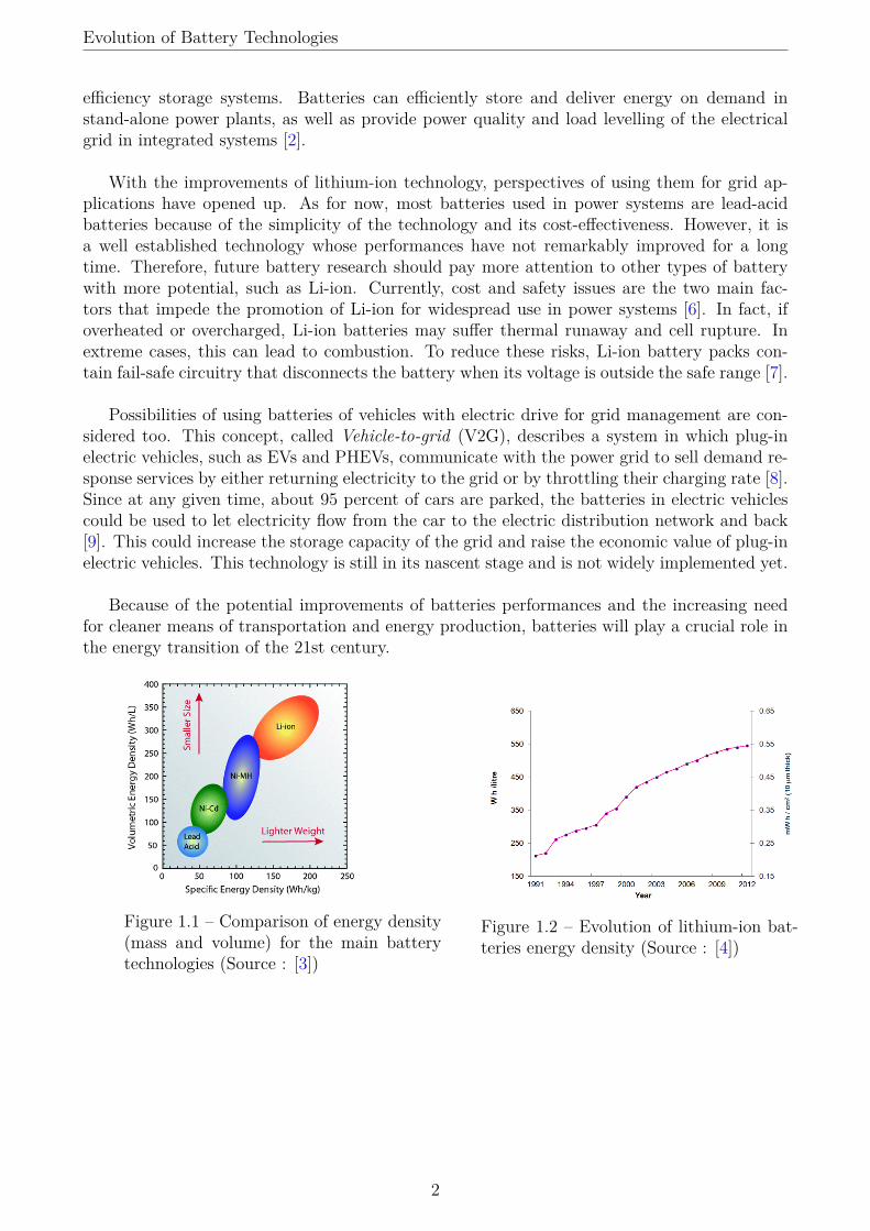
As for now, lithium-ion batteries are mostly used for small portable technology devicesbecause of their high energy density. Figure 1.1 shows how the different battery technologiescompare to each other in terms of density. Lithium-ion batteries are characterized by highspecific energy, high efficiency and long life [2]. Even if lithium-ion is the most expensive bat-tery technology, its price has been decreasing since it was first commercialized and is expectedto keep decreasing in the future, as shown in Figure 1.3. Meanwhile, the energy density ofthose batteries has been constantly increasing as shown in Figure 1.2. As a result, Li-ion bat-teries are now used for larger scale applications such as electric vehicles and even electrical grids.
Most electric vehicles batteries use Li-ion technology. The capacity of those batteries canreach up to 100 kWh. The price of the battery makes up around 35% of the vehicle price [5].The expected decrease in lithium-ion battery cost should make electric vehicles more affordablein the forthcoming years.The air pollution problem in large urban areas, may be only solved byreplacing internal combustion engine (ICE) cars with ideally, zero emission vehicles, i.e. elec-tric vehicles (EVs) or, at least, by controlled emission vehicles, i.e. full hybrid electric vehicles(HEVs) and/or plug-in electric vehicles (PHEVs) [2]. This will also decrease the total CO2emission, especially if the electricity is produced with renewable energies.
At the same time, investments for the exploitation of renewable energy resources are in-creasing worldwide, with particular attention to wind and solar power energy plants, whichare the most mature technologies. The intermittence of theses resources requires high energy
1
Evolution of Battery Technologies
efficiency storage systems. Batteries can efficiently store and deliver energy on demand instand-alone power plants, as well as provide power quality and load levelling of the electricalgrid in integrated systems [2].
With the improvements of lithium-ion technology, perspectives of using them for grid ap-plications have opened up. As for now, most batteries used in power systems are lead-acidbatteries because of the simplicity of the technology and its cost-effectiveness. However, it isa well established technology whose performances have not remarkably improved for a longtime. Therefore, future battery research should pay more attention to other types of batterywith more potential, such as Li-ion. Currently, cost and safety issues are the two main fac-tors that impede the promotion of Li-ion for widespread use in power systems [6]. In fact, ifoverheated or overcharged, Li-ion batteries may suffer thermal runaway and cell rupture. Inextreme cases, this can lead to combustion. To reduce these risks, Li-ion battery packs con-tain fail-safe circuitry that disconnects the battery when its voltage is outside the safe range [7].
Possibilities of using batteries of vehicles with electric drive for grid management are con-sidered too. This concept, called Vehicle-to-grid (V2G), describes a system in which plug-inelectric vehicles, such as EVs and PHEVs, communicate with the power grid to sell demand re-sponse services by either returning electricity to the grid or by throttling their charging rate [8].Since at any given time, about 95 percent of cars are parked, the batteries in electric vehiclescould be used to let electricity flow from the car to the electric distribution network and back[9]. This could increase the storage capacity of the grid and raise the economic value of plug-inelectric vehicles. This technology is still in its nascent stage and is not widely implemented yet.
Because of the potential improvements of batteries performances and the increasing needfor cleaner means of transportation and energy production, batteries will play a crucial role inthe energy transition of the 21st century.
Figure 1.1 – Comparison of energy density(mass and volume) for the main batterytechnologies (Source : [3])
Figure 1.2 – Evolution of lithium-ion bat-teries energy density (Source : [4])
2

Microgrids
Figure 1.3 – Cost predictions for automotive lithium-ion battery packs
1.2 Microgrids
1.2.1 Concepts of MicrogridsPower generation in the traditional power grid is very centralized, with power flowing uni-
directionally from large synchronous generators through a transmission/distribution networkto end-users. However, the environmental issues caused by the combustion of fossil fuels havestimulated research and development into new means of producing electricity and organizingthe power grid. With the emergence of distributed energy resource (DER) units, e.g., wind,photovoltaic (PV), battery, biomass, micro-turbine, fuel cell, etc., microgrid technologies haveattracted increasing attention as an effective mean of integrating such DER units into powersystems.
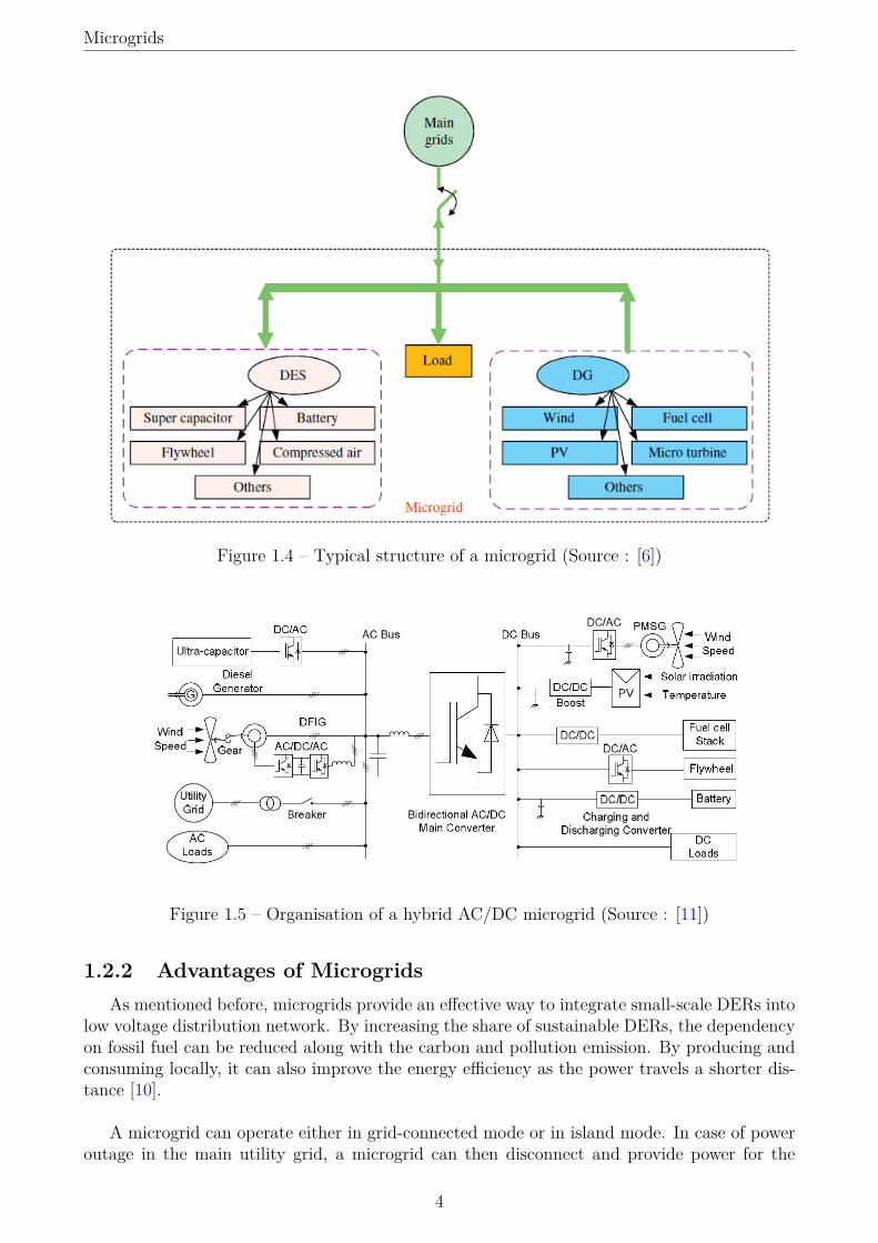
The U.S. Departement of Energy defines a microgrid as "a group of interconnected loads anddistributed energy resources within clearly defined electrical boundaries that acts as a singlecontrollable entity with respect to the grid. A microgrid can connect and disconnect from thegrid to enable it to operate in both grid-connected or island mode" [10]. The purpose of thisconcept is to develop a platform that facilitates the integration of distributed generators (DG),energy storage systems (ESS) and loads to ensure that the power grid can supply sustainable,price-competitive and reliable electricity. Figure 1.4 shows a typical microgrid structure withDG sources such as PV systems, wind turbine systems, microturbines and distributed energystorage (DES) facilities such as battery banks, supercapacitors, flywheels, etc. DES play anessential role in microgrids by smoothing the fluctuations of power from the DG units and byimproving the stability of the microgrid.
Microgrids can be classified as AC and DC type. Historically, AC has been the choice for overa hundred years due to easy transformation at different voltage levels and power transmissionover long distances as well as inherent characteristic from fossil energy driven rotating machines[11]. Since then, the advance in power electronics and the increase in DC loads has made DCpower grids an interesting choice. In the traditional AC grid, DC loads are connected to thegrid through a AC/DC rectifier. Another posssibility is to have a hybrid AC/DC microgridas shown in Figure 1.5. This allows to reduce the total number of converters by connectingDC loads to the DC grid and AC loads to the AC grid. The main converter is bidirectionaland allows power flow between the AC and DC grids. In grid-tied mode, the AC microgrid isconnected to the main utility grid at the point of common coupling (PCC).
3
Microgrids
Figure 1.4 – Typical structure of a microgrid (Source : [6])
Figure 1.5 – Organisation of a hybrid AC/DC microgrid (Source : [11])
1.2.2 Advantages of MicrogridsAs mentioned before, microgrids provide an effective way to integrate small-scale DERs into
low voltage distribution network. By increasing the share of sustainable DERs, the dependencyon fossil fuel can be reduced along with the carbon and pollution emission. By producing andconsuming locally, it can also improve the energy efficiency as the power travels a shorter dis-tance [10].
A microgrid can operate either in grid-connected mode or in island mode. In case of poweroutage in the main utility grid, a microgrid can then disconnect and provide power for the
4

Microgrids
local loads. It can thus give an improved level of reliability for end-users. Moreover, by usinglocal control of the DG facilities, the power quality can be enhanced and the fluctuations of in-termittent sources can be effectively compensated. Promoting customer participation throughdemand-side management is another way of improving quality and reliability of energy sup-ply. Recent development of Smart Grid technologies take advantage of the progress in elec-tronic communication technology to improve the efficiency of the grid by using features such asdemand-side management. Microgrids are an interesting platform to develop the Smart Gridtechnologies [10].
Finally, in addition to handling locally sensitive loads and the variability of renewablesources, microgrids can also provide ancillary servives to the main utility grid, such as fre-quency and voltage regulation, black start support and load balancing services. In this way,microgrids represent economic opportunities by compensation of these services to the bulk gridvia payments [6].
1.2.3 Challenges for MicrogridsWhile microgrids and larger integration of DG sources solve a lot of problems, new challenges
arise that need to be adressed in order to ensure that the present levels of reliability are notsignificantly affected and the potential benefits of DG units are fully harnessed. Those are thefollowing :
• Bidirectional power flows : While the power only flows unidirectionally from highvoltage to low voltage levels in the traditional power grid, the presence of DG units atlow voltage can cause reverse power flows which may lead to complications in protectioncoordination, undesirable power flow patterns, fault current distribution, and voltagecontrol [12].
• Stability : Local oscillations may emerge from the interaction of the control systems ofDG units, requiring a thorough small-disturbance stability analysis. Moreover, transientstability analysis are required to ensure seamless transition between the grid-connectedand stand-alone modes of operation in a microgrid [12].
• Modeling : Prevalence of three-phase balanced conditions, primarily inductive trans-mission lines, and constant-power loads are typically valid assumptions when modelingconventional power systems at a transmission level ; however, these do not necessarilyhold valid for microgrids, and consequently models need to be revised [12].
• Low inertia : Unlike bulk power systems where high number of synchronous generatorsensures a relatively large inertia, microgrids might show a low-inertia characteristic,especially if there is a significant share of power electronic-interfaced DG units. Althoughsuch an interface can enhance the system dynamic performance, the low inertia in thesystem can lead to severe frequency deviations in stand-alone operation if a propercontrol mechanism is not implemented [12].
• Uncertainty : The economical and reliable operation of microgrids requires a certainlevel of coordination among different DERs. This coordination becomes more challengingin isolated microgrids, where the critical demand-supply balance and typically highercomponent failure rates require solving a strongly coupled problem over an extendedhorizon, taking into account the uncertainty of parameters such as load profile andweather forecast. This uncertainty is higher than those in bulk power systems, due tothe reduced number of loads and highly correlated variations of available energy resources(limited averaging effect) [12].
5

Microgrids
1.2.4 Energy Storage Technology in MicrogridsEnergy storage technology facilitates high penetration of variable renewable energy re-
sources. ESS has been used for a long time in power systems but the integration of renewableenergy increases the demand for ESS. ESS can be divided into mechanical, electrochemical,chemical, electrical and thermal systems, as shown in Figure 1.6.
Figure 1.6 – Classification of energy storage systems (Source : Fraunhofer ISE)
The mechanical ESS are :• Pumped hydro : Energy is stored in the form of gravitational potential energy, pumped
from a lower elevation reservoir to a higher reservoir. Energy is retrieved by releasing thewater from the higher reservoir through a turbine, generating electricity. The reservoirscan either be natural or artificial. As for now, it represents the largest capacity of energystorage technology with 96% of all active tracked storage installations worldwide and atotal capacity of 168 GW [13].
• Compressed air : Energy is stored by compressing air into a reservoir and is retrievedby expanding the air through a turbine.
• Flywheel : A flywheel is a disk with a certain amount of mass that can spin to storeenergy in kinetic form. In order to minimize friction, a vacuum environment is usuallymade for the flywheel to spin in to ensure there is no air resistance. Magnetic or electro-magnetic bearings can also be used to make the spinning rotor float to make sure thereis no contact friction as with mechanical bearings [6].
The electrochemical ESS are :• Batteries : Most batteries are rechargeable batteries, also called secondary batteries.
They are composed of one or more electrochemical cells. It accumulates and storesenergy through a reversible electrochemical reaction. Several different combinationsof electrode materials and electrolytes are used, including lead–acid, nickel-cadmium(NiCd), nickel-metal hydride (NiMH) and lithium-ion (Li-ion).
• Fuel cells : This device converts the chemical energy from a fuel into electricity througha chemical reaction of positively charged hydrogen ions with oxygen or another oxidizingagent. Fuel cells are different from batteries in requiring a continuous source of fuel andoxygen or air to sustain the chemical reaction, whereas in a battery the chemicals presentin the battery react with each other to generate an electromotive force (emf) [14].
The electrical ESS are :• Supercapacitors : They have much higher capacitance, hence storage capacity, than
regular capacitors. Supercapacitors rely on the separation of charge at an electric inter-face that is measured in fractions of a nanometer, compared with micrometers for mostpolymer film capacitors. Energy storage is by means of static charge rather than of anelectrochemical process inherent to batteries [15].
6
Simulink Model and Real-time Simulations
• Superconducting Magnetic Energy Storage (SMES) : The basis of SMES is thestorage of energy in the magnetic field of a DC current flowing in superconducting coils.Energy losses are effectively zero because superconductors offer no resistance to electronflow [15].
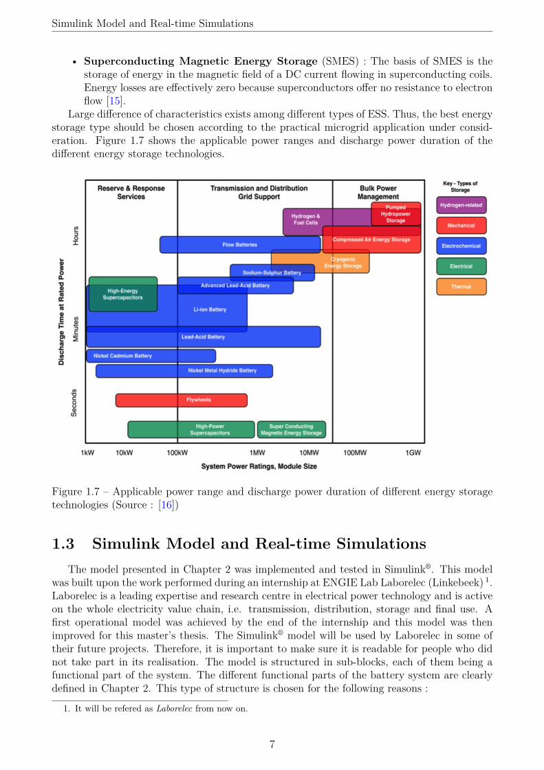
Large difference of characteristics exists among different types of ESS. Thus, the best energystorage type should be chosen according to the practical microgrid application under consid-eration. Figure 1.7 shows the applicable power ranges and discharge power duration of thedifferent energy storage technologies.
Figure 1.7 – Applicable power range and discharge power duration of different energy storagetechnologies (Source : [16])
1.3 Simulink Model and Real-time SimulationsThe model presented in Chapter 2 was implemented and tested in Simulink®. This model
was built upon the work performed during an internship at ENGIE Lab Laborelec (Linkebeek) 1.Laborelec is a leading expertise and research centre in electrical power technology and is activeon the whole electricity value chain, i.e. transmission, distribution, storage and final use. Afirst operational model was achieved by the end of the internship and this model was thenimproved for this master’s thesis. The Simulink® model will be used by Laborelec in some oftheir future projects. Therefore, it is important to make sure it is readable for people who didnot take part in its realisation. The model is structured in sub-blocks, each of them being afunctional part of the system. The different functional parts of the battery system are clearlydefined in Chapter 2. This type of structure is chosen for the following reasons :
1. It will be refered as Laborelec from now on.
7

Simulink Model and Real-time Simulations
• It improves the readability of the model. Above a certain level of complexity, a Simulink®
model can quickly become incomprehensible, especially for someone who did not takepart in its realisation. This structure allows someone to use a sub-block as a black box,i.e. without having to fully understand how it works. However, each sub-block has tobe documented so that the user can comprehend how they operate, if desired.
• This structure also makes it possible for someone to extract a sub-block and use it fora different applications. Hence, this model enlarges the Simulink® sub-blocks library ofLaborelec.
In addition to the Simulink® tests, the model was simulated in a real-time environment.Laborelec is in possession of a real-time simulator, called PHIL (Power Hardware In the Loop).The PHIL works with a software named RT-Lab®. RT-Lab® is a toolbox that, with some adap-tations, allows to run a Simulink® model in real-time.
Figure 1.8 illustrates the difference between offline and real-time simulation. During adiscrete-time simulation, the amount of real time required to compute all equations repre-senting a system during a given time step may be shorter or longer than the duration of thesimulation time step. Figure 1.8 a) and b) respectively represent those two possibilities. Thesetwo situations are referred to as offline simulation. Considering the simulation uses fixed-sizetime steps, the moment at which a result becomes available is irrelevent. Conversely, duringreal-time simulation, the accuracy of computations not only depends upon precise dynamic rep-resentation of the system, but also on the length of time used to produce results. If simulatoroperations are not all achieved within the required fixed time-step, the real-time simulation isconsidered erroneous. This is commonly known as an overrun [17].
Figure 1.8 c) illustrates the chronological principle of real-time simulation. For a real-timesimulation to be valid, the real-time simulator used must accurately produce the internal vari-ables and outputs of the simulation within the same length of time that its physical counterpartwould. This permits the real-time simulator to perform all operations necessary to make a real-time simulation relevant, including driving inputs and outputs (I/O) to and from externallyconnected devices. In this way, hadrware can be integrated in the loop an be part of thereal-time simulation. Running the battery model in real-time also validates the feasability ofthe controllers developed in this thesis. In fact, if the model can work without overruns, thedesigned controllers can be implemented and integrated in a physical system.
In order for the battery model to run without overruns, its computational cost had to berestrained. Threrefore, two models were developed for each converter (DC/DC and DC/AC,refer to Chapter 2) :
• A full model where the switching devices of the converter are represented. Hence, thismodel has to be simulated with a relatively small time step.
• An average dynamic model where the currents and voltages are averaged over one switch-ing period of the converter. In this way, the dynamics in the time order of a switchingperiod is not represented but the slower dynamics is modelled. The time step used canthen be larger.
The real-time simuations were successfully performed with the average dynamic models.
8

Simulink Model and Real-time Simulations
Figure 1.8 – Comparison between offline and real-time simulation (Source : [17])
In addition to that, it was initially planned to run some hardware tests as part of this the-sis. Laborelec owns a SAFT Li-ion battery which is adapted for power systems. Due to severalsetbacks, no tests could be carried out in time to validate the model. However, Laborelec hadpreviously tested the battery to evaluate its general characteristics. Some of the numericalvalues used to test the model with Simulink® are based on the given characteristics of thisSAFT battery.
In the future, Laborelec will further validate and use this model as part of projects they areinvolved in and integrate it in their real-time simulations. For example, ELECTRA Web-of-cellsis an European project in which Laborelec takes part with many other laboratories. The goalof this project is to study the concept of Web-of-Cells which is a decentralized real-time controlconcept, where the power system is divided in small cells, and where the need for reservesactivations as well as the activations themselves are dealt with in a decentralized manner bycell system operators [18]. This decentralized scheme aims to ancipate the new challenges forpower systems :
• More generation from intermittent renewable energy resources resulting in generationforecast errors and reduced generation dispatchability
• More distribution grid connected generation inducing reverse powerflows instead ofdownstream power distribution, congestions and voltage problems
• Increase of elctrical loads due to electrification of heating and transport
9

Chapter 2
Model of a Li-ion Battery EnergyStorage System
2.1 OverviewBefore going into the details of each component of a BESS, it is important to have a view
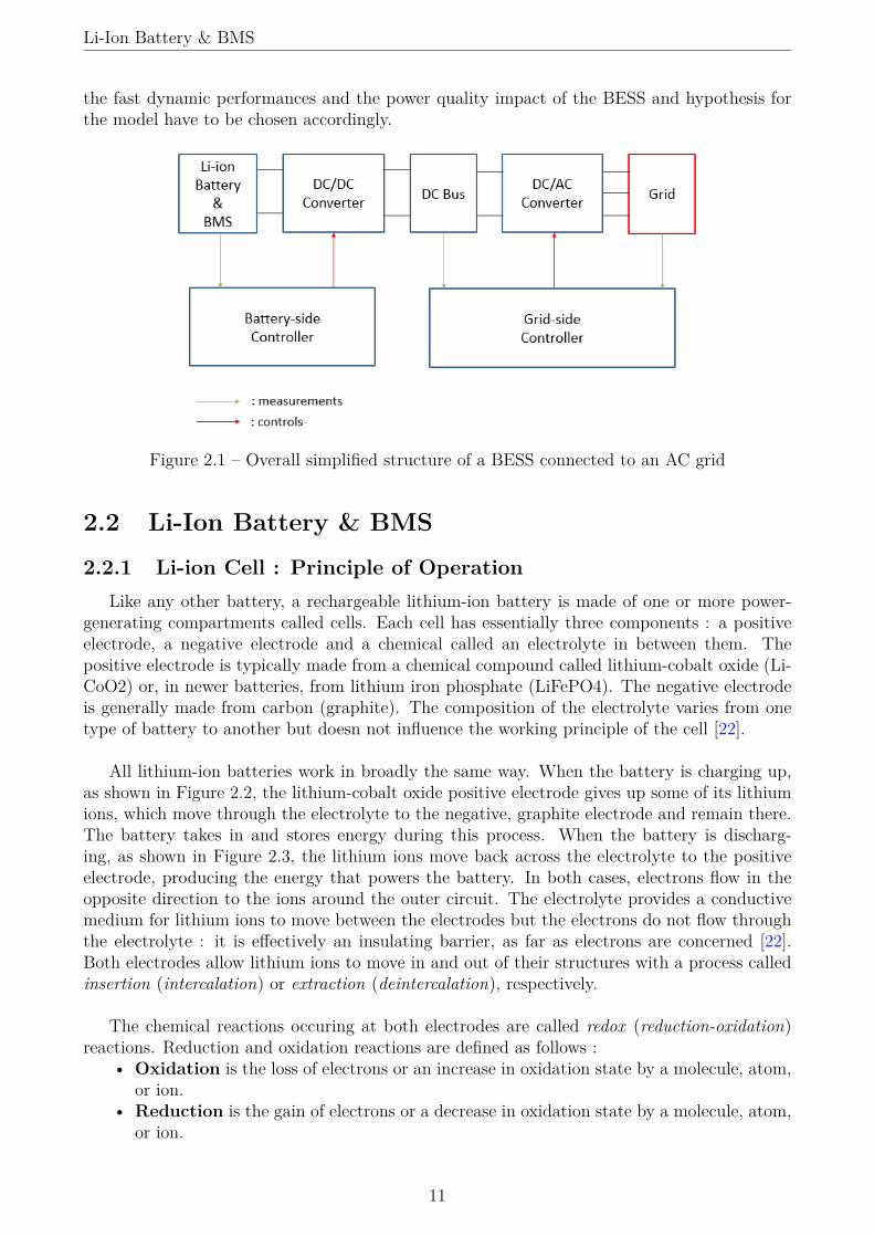
of its overall structure, represented in Figure 2.1. The elements composing the battery-side ofthe system are the following :
• Li-ion battery & BMS : A battery is the assembly of electrochemical cells mountedin series and in parallel. The BMS (Battery Management System) coordinates theinteractions of all the cells of a battery and gives information about the state of thebattery [19]. A BESS can be composed of one or multiple battery packs, each onehaving its own BMS.
• DC/DC converter : This converter allows the power to flow from the battery to theDC bus or the other way around. Hence, it must be bidirectional. The battery is usuallyat lower voltage than the DC bus.
• Battery-side controller : This controller acts on the DC/DC converter to regulatethe power flowing from/into the battery.
The DC bus is formed of a large capacitance. The voltage is controlled to be kept at a referencevalue such that the BESS can be connected to the grid through an AC/DC converter, despitethe voltage variations at the ouptput of the battery. In fact, the DC bus capacitor acts as afilter. Other utilities such as PV panels or wind turbines can be connected to the same DCbus.
The elements composing the grid-side of the system are the following :• DC/AC converter : The DC/AC converter connects the DC bus to the AC grid. In
the case of a BESS, this converter also has to be bidirectional.• Grid-side controller : This controller acts on the DC/AC converter to regulate the
DC bus voltage and consequently the power flowing from/into the grid.The system has to be modelled with a certain level of accuracy and complexity. When doing
a model for simulations, there is always a trade-off between :• A complex model that depicts accurately the physical phenomena• A simple model that has a low simulation costBefore going into the precise modelling of the different parts of the system, it is important to
define the scope of the model in order to make the right hypothesis. The purpose of the modelis to examine the interactions between a Li-ion BESS and a microgrid and more specificallyhow the BESS affects the reliability and quality of the power delivered in the microgrid. Theperturbations that a microgrid has to face can occur in a short time lapse. For instance, avoltage dip can be as short as one half-cycle (10 ms) [20]. Thus, the model has to emphasize
10
Li-Ion Battery & BMS
the fast dynamic performances and the power quality impact of the BESS and hypothesis forthe model have to be chosen accordingly.
Figure 2.1 – Overall simplified structure of a BESS connected to an AC grid
2.2 Li-Ion Battery & BMS
2.2.1 Li-ion Cell : Principle of OperationLike any other battery, a rechargeable lithium-ion battery is made of one or more power-
generating compartments called cells. Each cell has essentially three components : a positiveelectrode, a negative electrode and a chemical called an electrolyte in between them. Thepositive electrode is typically made from a chemical compound called lithium-cobalt oxide (Li-CoO2) or, in newer batteries, from lithium iron phosphate (LiFePO4). The negative electrodeis generally made from carbon (graphite). The composition of the electrolyte varies from onetype of battery to another but doesn not influence the working principle of the cell [22].
All lithium-ion batteries work in broadly the same way. When the battery is charging up,as shown in Figure 2.2, the lithium-cobalt oxide positive electrode gives up some of its lithiumions, which move through the electrolyte to the negative, graphite electrode and remain there.The battery takes in and stores energy during this process. When the battery is discharg-ing, as shown in Figure 2.3, the lithium ions move back across the electrolyte to the positiveelectrode, producing the energy that powers the battery. In both cases, electrons flow in theopposite direction to the ions around the outer circuit. The electrolyte provides a conductivemedium for lithium ions to move between the electrodes but the electrons do not flow throughthe electrolyte : it is effectively an insulating barrier, as far as electrons are concerned [22].Both electrodes allow lithium ions to move in and out of their structures with a process calledinsertion (intercalation) or extraction (deintercalation), respectively.
The chemical reactions occuring at both electrodes are called redox (reduction-oxidation)reactions. Reduction and oxidation reactions are defined as follows :
• Oxidation is the loss of electrons or an increase in oxidation state by a molecule, atom,or ion.
• Reduction is the gain of electrons or a decrease in oxidation state by a molecule, atom,or ion.
11

Li-Ion Battery & BMS
The positive (cathode) electrode half-reaction in the lithium-doped cobalt oxide substrate is(left : reduction, right : oxidation) [23]:
CoO2 + Li+ + e− LiCoO2
The negative (anode) electrode half-reaction for the graphite is (left : oxidation, right : reduc-tion) :
LiC6 C6 + Li+ + e−
The full reaction (left : charge, right : discharge) being :
LiC6 + CoO2 C6 + LiCoO2
The net electromotive force of the full reaction is the difference between the reduction potentialsof both half-reactions. The emf of a cell depends thus on the chemical reactions of its electrodesand electrolytes. Alkaline and zinc–carbon cells have different chemistries, but approximatelythe same emf of 1.5 volts; likewise NiCd and NiMH cells have different chemistries, but approx-imately the same emf of 1.2 volts. The high electrochemical potential changes in the reactionsof lithium compounds give lithium cells emfs of 3 volts or more [24].
The electrical driving force ∆Vbat across the terminals of a cell is known as the terminalvoltage (difference) and is measured in volts. The terminal voltage of a cell that is neithercharging nor discharging is called the open-circuit voltage and equals the emf of the cell. Becauseof internal resistance, the terminal voltage of a cell that is discharging is smaller in magnitudethan the open-circuit voltage and the terminal voltage of a cell that is charging exceeds theopen-circuit voltage.
Figure 2.2 – Li-ion cell charging mecha-nism (Source : [21])
Figure 2.3 – Li-ion cell discharging mech-anism (Source : [21])
2.2.2 Battery Management SystemA battery or battery pack is a collection of cells which are ready for use, as it contains an
appropriate housing, electrical interconnections, and possibly electronics to control and protectthe cells from failure. The term module is often used as an intermediate topology , with theunderstanding that a battery pack is made of modules, and modules are composed of individualcells [25].
12
Li-Ion Battery & BMS
The BMS is required to coordinate the operation of the cells forming the battery. In fact,a battery is indissociable from its BMS as it cannot work properly without it. The objectiveof the BMS is to provide protection, increase the lifespan and maintain the stability of thebatteries in the BESS. In order to accomplish these tasks, the BMS should have the functionsof monitoring, computation, control and communication [6].
To protect the batteries from damage and maintain them in good condition, the BMS needsto monitor the temperature, voltage and current in the battery. Overheating the battery isvery dangerous, and may lead to explosion and fire. Hence, temperature monitoring is veryimportant to ensure that the batteries work in stable conditions.
The BMS has to perform computations such as the state-of-charge (SOC) and state-of-health(SOH) of the battery based on the voltage and current measurements. The SOC correspondsto the energy stored by the battery over the total energy it is able to store. The SOH is afigure of merit of the condition of a battery compared to its initial conditions. The definition ofthe SOH is more ambiguous as the designer decides how it is computed. The estimation of theSOH usually depends on several measurements such as internal resistance, capacity, number ofcharge/discharge cycles and voltage with an arbitrary weight for each parameter [26].
The monitoring of the SOC allows to control the current accordingly so that overchargingor over-discharging can be prevented. Furthermore, the current of batteries should stay in asafe range, especially during the charging process. If the charging current is too high, it will notonly damage the battery’s health, but also causes accidents. The BMS has to be coordinatedwith the DC/DC converter as it controls the charging/discharging current.
Another responsibility of the BMS is to ensure cell balancing. In each battery package,several battery cells are connected in series to achieve a bigger capacity. However, the qualityor ability of each battery cell is not identical, which may result in imbalance among cells duringcharging or discharging. The imbalance among battery cells decreases the available energy ofthe overall battery package. Due to the safe range requirement of the battery’s SOC, it stopscharging or discharging when one of the cells reaches the limits. Therefore, for the unbalancedsituation, the battery package will not continue to charge or discharge when the battery cellwith the highest SOC reaches the upper limit or the battery cell with lowest SOC reaches thelower limit. One technique commonly used is called passive cell balancing. As shown in Figure2.4, the BMS commands field-effect transistors so that the cells with higher SOC recharge thecells with lower SOC [6].
13

Li-Ion Battery & BMS
Figure 2.4 – Passive cell balancing BMS (Source : [6])
2.2.3 Equivalent ModelThe goal of the model is to capture the characteristics of real-life batteries and predict
their behaviour under various operating conditions. Different types of models can be used withdifferent levels of accuracy.
Electrochemical models [27] can fully describe the behaviour of a battery with equationsthat capture the chemical phenomena occuring in the battery. However, these models aretypically computationally time-consuming due to a system of coupled time-varying partial dif-ferential equations. Such models are best suited for optimization of the physical design aspectsof electrodes and electrolyte [28].
Mathematical models [29] use stochastic approaches or empirical equations which can pre-dict runtime, efficiency and capacity. However, these models are inaccurate (5-20% error) andhave no direct relation between model parameters and the I-V characteristics of batteries. Asa result, they have limited value in circuit simulation software [28] and consequently for gridapplications.
Electrical models are the most intuitive for use in circuit simulation. The battery can berepresented as an equivalent circuit where the number of elements in the circuit defines thecomplexity of the model. The use of RC parallel networks allows to model with accuracy thedynamic behaviour of the battery. However, electrical models are not the best at evaluatingthe runtime and the SOC of the battery. The emphasis of this model is intentionally placed onthe dynamic performances.
The electrical model used is represented in Figure 2.5. The choice is to use two RC parallelnetworks in addition to the constant resistance Rseries and the voltage source Voc which cor-responds to the open-circuit voltage of the battery. The first parallel Rt,sCt,s network modelsthe faster transient of the battery with a time constant τsec in the order of one second [28].The second parallel Rt,mCt,m network models the slower transient of the battery with a timeconstant τmin in the order of one minute [28]. Some articles [28, 30] use additional RC net-
14

Li-Ion Battery & BMS
works with longer time constants (more than one hour) but it is not necessary for the aimedapplication ; using two RC networks is a good trade-off between precision and computationalcost. The open-circuit voltage as well as the resistances and capacitances depend on the SOC.
Figure 2.5 – Electrical model of a Li-ion battery
The parameters of the model are as follows :
Vbat Battery output voltage [V]Voc Battery open-circuit voltage [V]Zeq Equivalent parasitic impedance [Ω]Ibat Battery current[A]SOC State-of-charge [/]SOCinit Initial state-of-charge [/]Cbat Battery capacity [A s]
where Zeq is the sum of Rseries and the two RC networks. The equations of the model arethe following :
SOC(t) = SOCinit −∫ t
0
Ibat(t)Cbat
(2.1)
Vbat = Voc − IbatZeq (2.2)where Ibat is positive if the battery is discharging and negative if charging. The relationsbetween the parameters and the SOC also have to be determined to complete the model. Thechoice made in Article [28] is to use polynomial functions of 6th order. For instance, the relationbetween Voc and SOC is :
Voc = A0 + A1 ·SOC + A2 ·SOC2 + ... + A6 ·SOC6 (2.3)
The same type of relation is used for the resistances and capacitances. All the coefficients ofthe polynomial functions are determined experimentally.
A few assumptions are made for the model, for the sake of simplicity and based on theaimed application for the model :
• The effect of capacity fading is neglected. Capacity fading refers to the irreversible lossof usable capacity of a battery due to time, temperature and cycle number. Generally, abattery is considered to be usable until reaching 70% of its initial capacity. This point isreached after roughly 2000 Full Equivalent Cycles (FEC) for Li-Ion batteries used in EVor ESS [32]. Considering the goal of the model is to study the relatively fast dynamicsof a battery, it is a reasonable assumption to neglect this long term effect. The capacityof the battery is thus considered to be constant during the simulation.
15

Li-Ion Battery & BMS
• The effect of temperature is also neglected which is equivalent to considering that thetemperature is constant. In addition to influencing the lifetime of the battery, tempera-ture has an effect on the open-circuit voltage Voc. The temperature of the battery packis controlled by its cooling system. The operation of most Li-ion cell is limited to atemperature of 20°C to 40°C [31]. Figure 2.6 shows that higher temperature causes verylittle alteration on a typical Li-ion cell compared to room temperature.
• The effect of self-discharge is neglected. This effect causes the SOC decrease even whenthe battery is in off-mode. For Li-ion, the energy loss is typically asymptotical, with 5%in 24h after charge and then 1-2% per month (plus 3% for safety circuit) [33].
Figure 2.6 – Open-circuit voltage Voc of a Li-ion cell vs SOC for different temperatures (Source: [28])
The efficiency of the battery is taken into account through the resistors of the model asthey dissipate power. The BMS also intervenes, in cooperation with the DC/DC converter,in the behaviour of the battery. The BMS limits the maximal charge/discharge current of thebattery. It also takes control of the current when the SOC is about 90% or 10% to avoidovercharge/over-discharge [6].
2.2.4 Example and TestsAs mentioned in Section 1.3, it was initially planned to perform experimental tests on a
SAFT Li-ion battery to identify the parameters of the model. However, due to several setbacks,these tests could not be carried out. From then on, the results obtained in Article [28] (quoted269 times) are utilized to build a realistic battery model, as it is one of the few articles whoanalyzes thoroughly the fast dynamic characteristics of Li-ion batteries. This article identifiesthe parameters for a single Panasonic CGR18650A Li-ion cell. The specifications of this cellare given in Table 2.1 [34].
Nominal Voltage 3.7 VCapacity 2.2 Ah
Max. charge current 1.5 A (0.7 C 1)Max. discharge current 2.2 A (1 C)
Table 2.1 – Specifications of a Panasonic CGR18650A Li-ion cell
1. Currents for batteries are often expressed in C-rate where 1C corresponds to the current that the batterycan provide during 1 hour
16

Li-Ion Battery & BMS
From there, the battery pack with the desired nominal voltage and capacity can be built bymounting nparallel branches in parallel, each one containing nseries cells in series. For a batterywith a nominal voltage Vnom = 430 V and a capacity of Cbat = 34kWh, the specifications aregiven in Table 2.2 2.
nseries 116nparallel 36
Nominal Voltage 430 VCapacity 34kWh
Max. continuous charge current 56 A (0.7 C)Max. continuous discharge current 80 A (1 C)
Nominal power 25kW (0.7 C)
Table 2.2 – Specifications of a 25kW/34kWh Li-ion battery
On the basis of the data given in Article [28] for one Li-ion cell, the coefficients of thepolynomial functions (Eq 2.3) can be computed for the whole battery pack. The resultingfunctions are shown in Figures 2.7-2.10.
SOC[/]
0 0.1 0.2 0.3 0.4 0.5 0.6 0.7 0.8 0.9 1
Vo
c[V
]
300
320
340
360
380
400
420
440
460
480
Figure 2.7 – Voc vs SOC
SOC[/]
0 0.1 0.2 0.3 0.4 0.5 0.6 0.7 0.8 0.9 1
Reis
tances[Ω
]
0
0.1
0.2
0.3
0.4
0.5
0.6
0.7
0.8
0.9
1
Rser
Rt,s
Rt,m
Figure 2.8 – Rser, Rt,s & Rt,m vs SOC
2. These specifications correspond roughly to those of the SAFT Li-ion battery used by ENGIE Lab Laborelec(Linkebeek) for grid applications
17
DC/DC Converter and Battery-side Controller
SOC[/]
0 0.1 0.2 0.3 0.4 0.5 0.6 0.7 0.8 0.9 1
τse
c[s
]
0.02
0.03
0.04
0.05
0.06
0.07
0.08
0.09
0.1
0.11
0.12
Figure 2.9 – τsec = Rt,sCt,s vs SOC
SOC[/]
0 0.1 0.2 0.3 0.4 0.5 0.6 0.7 0.8 0.9 1
τm
in[s
]
40
50
60
70
80
90
100
110
120
130
Figure 2.10 – τmin = Rt,mCt,m vs SOC
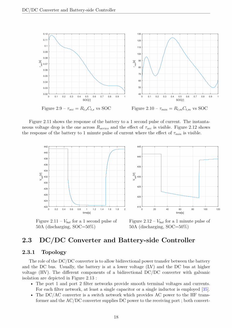
Figure 2.11 shows the response of the battery to a 1 second pulse of current. The instanta-neous voltage drop is the one across Rseries and the effect of τsec is visible. Figure 2.12 showsthe response of the battery to 1 minute pulse of current where the effect of τmin is visible.
time[s]
0 0.2 0.4 0.6 0.8 1 1.2 1.4 1.6 1.8 2
Vb
at[V
]
422
424
426
428
430
432
434
436
438
440
442
Figure 2.11 – Vbat for a 1 second pulse of50A (discharging, SOC=50%)
time[s]
0 20 40 60 80 100 120
Vb
at[V
]
415
420
425
430
435
440
445
Figure 2.12 – Vbat for a 1 minute pulse of50A (discharging, SOC=50%)
2.3 DC/DC Converter and Battery-side Controller
2.3.1 TopologyThe role of the DC/DC converter is to allow bidirectional power transfer between the battery
and the DC bus. Usually, the battery is at a lower voltage (LV) and the DC bus at highervoltage (HV). The different components of a bidirectional DC/DC converter with galvanicisolation are depicted in Figure 2.13 :
• The port 1 and port 2 filter networks provide smooth terminal voltages and currents.For each filter network, at least a single capacitor or a single inductor is employed [35].
• The DC/AC converter is a switch network which provides AC power to the HF trans-former and the AC/DC converter supplies DC power to the receiving port ; both convert-
18
DC/DC Converter and Battery-side Controller
ers must allow for bidirectional power transfer. Typically, full bridge circuits, half-bridgecircuits, and push-pull circuits are employed. However, different solutions (e.g. the singleswitch networks used in a bidirectional flyback converter) are reported, as well [35, 36].
• The reactive HF networks provide energy storage capability within the HF AC part.Even if these parts are not necessarily required for a fully functional bidirectional DC/DCconverter, they will always be present in practice due to the parasitic components of theHF transformer (e.g. stray and magnetizing inductances, parasitic capacitances) [35].
• The HF transformer is required in order to achieve electric isolation; it further enableslarge voltage and current transfer ratios. The HF transformer is considered superior overa low frequency transformer, since transformer and filter components become smaller(and often less expensive) at higher frequencies. However, increasing the switchingfrequency increases the switching losses in the semiconductors [35].
Figure 2.13 – General topology of an isolated, bidirectional DC–DC converter (Source : [35])
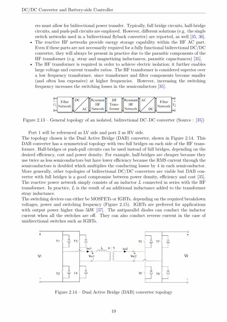
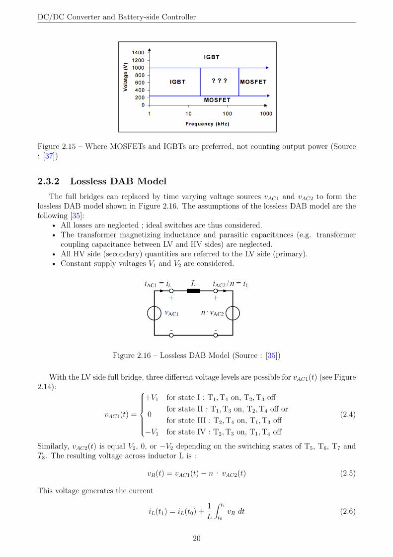
Port 1 will be referenced as LV side and port 2 as HV side.The topology chosen is the Dual Active Bridge (DAB) converter, shown in Figure 2.14. ThisDAB converter has a symmetrical topology with two full bridges on each side of the HF trans-former. Half-bridges or push-pull circuits can be used instead of full bridges, depending on thedesired efficiency, cost and power density. For example, half-bridges are cheaper because theyuse twice as less semiconductors but have lower efficiency because the RMS current through thesemiconductors is doubled which multiplies the conducting losses by 4 in each semiconductor.More generally, other topologies of bidirectional DC/DC converters are viable but DAB con-verter with full bridges is a good compromise between power density, efficiency and cost [35].The reactive power network simply consists of an inductor L connected in series with the HFtransformer. In practice, L is the result of an additional inductance added to the transformerstray inductance.The switching devices can either be MOSFETs or IGBTs, depending on the required breakdownvoltages, power and switching frequency (Figure 2.15). IGBTs are preferred for applicationswith output power higher than 5kW [37]. The antiparallel diodes can conduct the inductorcurrent when all the switches are off. They can also conduct reverse current in the case ofunidirectional switches such as IGBTs.
Figure 2.14 – Dual Active Bridge (DAB) converter topology
19
DC/DC Converter and Battery-side Controller
Figure 2.15 – Where MOSFETs and IGBTs are preferred, not counting output power (Source: [37])
2.3.2 Lossless DAB ModelThe full bridges can replaced by time varying voltage sources vAC1 and vAC2 to form the
lossless DAB model shown in Figure 2.16. The assumptions of the lossless DAB model are thefollowing [35]:
• All losses are neglected ; ideal switches are thus considered.• The transformer magnetizing inductance and parasitic capacitances (e.g. transformer
coupling capacitance between LV and HV sides) are neglected.• All HV side (secondary) quantities are referred to the LV side (primary).• Constant supply voltages V1 and V2 are considered.
Figure 2.16 – Lossless DAB Model (Source : [35])
With the LV side full bridge, three different voltage levels are possible for vAC1(t) (see Figure2.14):
vAC1(t) =
+V1 for state I : T1,T4 on, T2,T3 off
0 for state II : T1,T3 on, T2,T4 off orfor state III : T2,T4 on, T1,T3 off
−V1 for state IV : T2,T3 on, T1,T4 off
(2.4)
Similarly, vAC2(t) is equal V2, 0, or −V2 depending on the switching states of T5, T6, T7 andT8. The resulting voltage across inductor L is :
vR(t) = vAC1(t)− n· vAC2(t) (2.5)
This voltage generates the current
iL(t1) = iL(t0) + 1L
∫ t1
t0vR dt (2.6)
20

DC/DC Converter and Battery-side Controller
at the time t1, starting with inital current iL(t0) at time t0. The voltage sources vAC1 and vAC2thus generate or receive the respective instantaneous powers
p1(t) = vAC1(t) · iL(t) and p2(t) = vAC2(t) · iL(t) (2.7)
The average power for one switching cycle Ts = 1/fs is
P1 = 1Ts
∫ t0+Ts
t0p1(t)dt (2.8)
for the LV side andP2 = 1
Ts
∫ t0+Ts
t0p2(t)dt (2.9)
for the HV side. Moreover, since the model is lossless :
P1 = P2 (2.10)
The power level of the DAB converter is typically adjusted using one or more out of the 4control parameters which are [35]:
• the phase shift, ϕ, between vAC1(t) and vAC2(t) with −π < ϕ ≤ π• the duty cycle, D1, of vAC1 with 0 ≤ D1 ≤ 1/2• the duty cycle, D2, of vAC2 with 0 ≤ D1 ≤ 1/2• the switching frequency fs
The simplest and most common modulation principle of a DAB converter, called phase shiftmodulation, is considered here. It operates with constant switching frequency and maximumduty cycles, D1 = D2 = 1/2; it solely varies the phase shift ϕ in order to control transferredpower. Hence, vAC1(t) is either +V1 or −V1 and vAC2(t) is either +V2 or −V2 as shown inFigure 2.17. In practice, as semiconductors have a finite switching time, D1 and D2 have to beslightly smaller than 1/2 to make sure that no arm of the bridges is short-circuited. However,considering that D1 = D2 = 1/2 simplifies the following calculations.
Figure 2.17 – Example of transformer voltages and inductor current waveforms with phase shiftmodulation (Source : [35])
21

DC/DC Converter and Battery-side Controller
During steady-state operation, the voltages vAC1(t) and vAC2(t) and the inductor currentrepeat every half-cycle with reversed signs :
vAC1(t+ Ts/2) = −vAC1(t)vAC2(t+ Ts/2) = −vAC2(t)iL(t+ Ts/2) = −iL(t)
(2.11)
Therefore, only the first half-cycle (intervals I and II in Figure 2.17) has to be considered forthe calculation of the transferred power. With t0 = 0 (2.8), we have
P1 = 1Ts
∫ Ts
0p1(t)dt = 2
Ts
∫ Ts/2
0vAC1(t) · iL(t)dt = 2V1
Ts
∫ Ts/2
0iL(t)dt (2.12)
where t0 is such that vAC1(t) = V1 during the whole half-cycle. In order to obtain an analyticalexpression for P1, the current iL(t) needs to be determined. In steady-state operation, a certaincurrent iL,0 = iL(t0) is presumed. On the assumption of a positive phase shift, 0 ≤ ϕ ≤ π, theresulting expressions for the inductor current are [35] :
time interval I : iL(t) = iL,0 + (V1 + nV2)t/L 0 ≤ t ≤ Tϕ
time interval II : iL(t) = iL(Tϕ) + (V1 − nV2)(t− Tϕ)/L Tϕ < t ≤ Ts/2(2.13)
Due to half-cycle symmetry (2.11) and with Tϕ = ϕ/(2πfs),
iL,0 = π(nV2 − V1)− 2ϕnV2
4πfsL(2.14)
is obtained for positive phase shift, 0 ≤ ϕ ≤ π, and the same result for negative phase shift,−π ≤ ϕ < 0. With 2.10 and 2.12, and by extending the results to the full phase shift range,−π < ϕ ≤ π the transferred power
P = P1 = P2 = nV1V2ϕ(π − |ϕ|)2π2fsL
− π < ϕ ≤ π (2.15)
is obtained where P > 0 if the power is transferred from the LV side to the HV side and P < 0if the power is transferred from the HV side to the LV side. The maximum power that can betransferred with phase shift modulation is then :
|Pmax| =nV1V2
8fsLfor ϕ = ±π/2 (2.16)
The maximum power is thus limited by the converter inductance L.
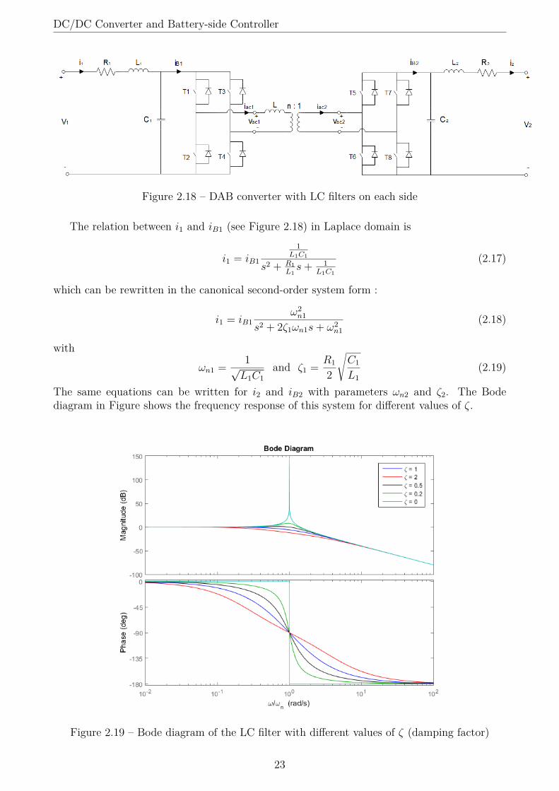
2.3.3 LC FiltersThe role of the filters is to smoothen the battery and DC bus currents by filtering the AC
component at the switching frequency. LC filters provide second-order filtering. Figure 2.18shows the DAB converter with LC filters on each side. Damping resistors are added to makesure that the system is not unstable.
22
DC/DC Converter and Battery-side Controller
Figure 2.18 – DAB converter with LC filters on each side
The relation between i1 and iB1 (see Figure 2.18) in Laplace domain is
i1 = iB1
1L1C1
s2 + R1L1s+ 1
L1C1
(2.17)
which can be rewritten in the canonical second-order system form :
i1 = iB1ω2
n1s2 + 2ζ1ωn1s+ ω2
n1(2.18)
withωn1 = 1√
L1C1and ζ1 = R1
2
√C1
L1(2.19)
The same equations can be written for i2 and iB2 with parameters ωn2 and ζ2. The Bodediagram in Figure shows the frequency response of this system for different values of ζ.
Figure 2.19 – Bode diagram of the LC filter with different values of ζ (damping factor)
23

DC/DC Converter and Battery-side Controller
The LC filters have to be designed such that
fs ωn1/2π and fs ωn2/2π (2.20)
where fs is the switching frequency of the converter, in order to effectively filter the AC com-ponent of frequency fs.
2.3.4 Average Dynamic ModelSimulating the entire converter with its switches has a big computational cost. In fact, with
the high switching frequency (typically in the range 10-100kHZ) of these converters and thehigh sensibility of the output power with respect to the phase shift ϕ, small time steps arerequired for the simulation to work properly.
Using an average dynamic model allows to obtain approximately the same input/outputcurrents and voltages without modelling the switches, hence highly reducing the computationalcost. The average dynamic model works by averaging the values of the currents and voltagesover one switching period. The slower dynamic of the LC filters it thus modelled but the fasterdynamic of the bridges is not taken into account as the AC component of frequency fs is filteredanyway.
Rewriting 2.15 for the DAB converter with LC filters (see Figure 2.18), the average powertransferred by each bridge over one switching period is
P = P1 = P2 = nVC1VC2ϕ(π − |ϕ|)2π2fsL
− π < ϕ ≤ π (2.21)
with VC1 and VC2 the voltages across capacitors C1 and C2. From there, the two bridges canbe replaced by controlled current sources (see Figure 2.20) with magnitudes
iB1 = P1
VC1= nVC2ϕ(π − |ϕ|)
2π2fsL− π < ϕ ≤ π (2.22)
iB2 = P2
VC2= nVC1ϕ(π − |ϕ|)
2π2fsL− π < ϕ ≤ π (2.23)
The average dynamic model and complete model are tested and compared in Subsection2.3.6.
Figure 2.20 – Average dynamic model of DAB converter
24

DC/DC Converter and Battery-side Controller
2.3.5 Battery-side ControllerThe battery-side controller acts on the control parameters of the DAB converter to control
the power transfer between the battery and the DC bus. In the case of phase shift modulation,only the phase shift is controlled. In practice, the modulation technique is adjusted dependingon the load. For example, Zero Current Switching (ZCS) can be obtained by having triangularor trapezoidal waveforms, hence decreasing the switching losses [35]. This is, however, notconsidered here. Figure 2.21 shows the resulting closed-loop system. The error Pref − P goesto a PI controller whose transfer function is
C(s) = KP + KI
s= G
τs+ 1τs
(2.24)
where KP = G is the proportional gain and KI = G/τ is the integral gain. Phase shift is keptin the interval −π/2 ≤ ϕ ≤ π/2 because the maximum power in absolute value is reached forϕ = ±π/2 and this interval minimizes the RMS current in the transformer.
Figure 2.21 – Closed-loop control scheme of the DAB converter
2.3.6 Example and TestsThe battery defined in subsection 2.2.4 is considered to be connected to the LV side of the
converter (port 1) and a DC bus of 700V is connected to the HV side (port 2). The DC busvoltage is considered here to be constant (ideal voltage source). The parameters chosen for theDAB converter are given in Table 2.3 (refer to Figure 2.18).
L 23µH fs 20kHzR1 0.1Ω R2 0.1ΩL1 0.1mH L2 0.1mHC1 1mF C2 1mFV1nom 430V V2nom 700Vn V1nom/V2nom = 0.61
Table 2.3 – Parameters of DAB converter
Since the nominal power of the battery is 25kW (>5kW), IGBTs are used as switchingdevices [37]. The choice of fs = 20kHz is realistic for IGBTs used in this power range [38].With that choice of parameters, the natural frequency of the LC filters is :
fn1 = fn2 = 12π√LC
= 503Hz
The influence of the DAB converter parameters is discussed in Appendix B. Figure 2.22shows the power curve of the lossless DAB for the chosen parameters (Equation 2.21). The
25

DC/DC Converter and Battery-side Controller
inductance L was chosen such that the converter can transfer a maximum power of 50kW, if itis necessary for a short duration. In this way, the normal operating area is in the more linearpart of the curve.
φ[deg]
-100 -80 -60 -40 -20 0 20 40 60 80 100
P[k
W]
-60
-40
-20
0
20
40
60
Figure 2.22 – P vs ϕ for VC1 = 430V and VC2 = 700V
Since this model is lossless, it does not directly computes the efficiency of the converter.However, it can be taken taken into account indirectly. This type of converter typically has anominal efficiency of about 95% [39]. Figure 2.23 shows the typical load-efficiency curve of aDAB converter. The efficiency is higher than 90% as long as the load is higher than 10% of themaximum load.
Figure 2.23 – Typical load-efficiency curve of a DAB converter (Source : [40])
Open-loop system
Figures 2.24-2.27 show the open-loop response to a phase shift step in terms of power atthe battery (LV) and at the DC bus (HV) for the complete model and the average dynamicmodel. The comparison shows that the average dynamic model (Figure 2.20) reproduces quiteaccurately the behaviour of the complete model (Figure 2.18). The transferred power has anovershoot and transient oscillations due to the LC filters. Figures 2.28-2.31 show the voltagesacross the capacitors C1 and C2. Figure 2.32 shows the current and voltages waveforms at thetransformer in steady-state.
26

DC/DC Converter and Battery-side Controller
In order for the simulations to work properly with the complete model, the duty cyclesD1 and D2 are set slightly smaller than 1/2 and the switches have conducting and snubberresistances. On top of that, the asymmetry between the two bridges may explain why there isa power transfer when ϕ is 0 (Figures 2.24 and 2.26).
time[s]
0 0.05 0.1 0.15 0.2 0.25 0.3
PL
V[k
W]
0
5
10
15
20
25
30
35
Figure 2.24 – PLV after a 20 phase shiftstep with complete model
time[s]
0 0.05 0.1 0.15 0.2 0.25 0.3
PL
V[k
W]
0
5
10
15
20
25
30
Figure 2.25 – PLV after a 20 phase shiftstep with average dynamic model
time[s]
0 0.05 0.1 0.15 0.2 0.25 0.3
PH
V[k
W]
0
5
10
15
20
25
30
Figure 2.26 – PHV after a 20 phase shiftstep with complete model
time[s]
0 0.05 0.1 0.15 0.2 0.25 0.3
PH
V[k
W]
0
5
10
15
20
25
30
Figure 2.27 – PHV after a 20 phase shiftstep with average dynamic model
27

DC/DC Converter and Battery-side Controller
time[s]
0 0.05 0.1 0.15 0.2 0.25 0.3
vC
1[V
]
422
424
426
428
430
432
434
436
438
440
Figure 2.28 – vC1 after a 20 phase shiftstep with complete model
time[s]
0 0.05 0.1 0.15 0.2 0.25 0.3
vC
1[V
]
422
424
426
428
430
432
434
436
438
440
442
Figure 2.29 – vC1 after a 20 phase shiftstep with average dynamic model
time[s]
0 0.05 0.1 0.15 0.2 0.25 0.3
vC
2[V
]
699
700
701
702
703
704
705
706
707
708
709
Figure 2.30 – vC2 after a 20 phase shiftstep with complete model
time[s]
0 0.05 0.1 0.15 0.2 0.25 0.3
vC
2[V
]
698
700
702
704
706
708
710
Figure 2.31 – vC2 after a 20 phase shiftstep with average dynamic model
time[s]
0.3832 0.3832 0.3833 0.3833 0.3833
Vo
lta
ge
[V], C
urr
en
t[A
]
-500
-400
-300
-200
-100
0
100
200
300
400
500
iL
vAC1
n vAC2
Figure 2.32 – Current and voltages waveforms (referred to LV side) at the transformer insteady-state
28
DC/DC Converter and Battery-side Controller
Closed-loop system
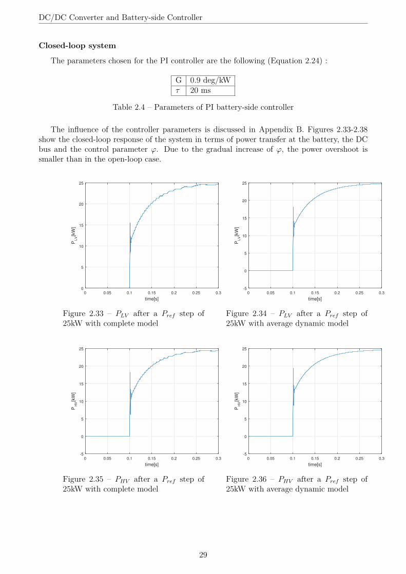
The parameters chosen for the PI controller are the following (Equation 2.24) :
G 0.9 deg/kWτ 20 ms
Table 2.4 – Parameters of PI battery-side controller
The influence of the controller parameters is discussed in Appendix B. Figures 2.33-2.38show the closed-loop response of the system in terms of power transfer at the battery, the DCbus and the control parameter ϕ. Due to the gradual increase of ϕ, the power overshoot issmaller than in the open-loop case.
time[s]
0 0.05 0.1 0.15 0.2 0.25 0.3
PL
V[k
W]
0
5
10
15
20
25
Figure 2.33 – PLV after a Pref step of25kW with complete model
time[s]
0 0.05 0.1 0.15 0.2 0.25 0.3
PL
V[k
W]
-5
0
5
10
15
20
25
Figure 2.34 – PLV after a Pref step of25kW with average dynamic model
time[s]
0 0.05 0.1 0.15 0.2 0.25 0.3
PH
V[k
W]
-5
0
5
10
15
20
25
Figure 2.35 – PHV after a Pref step of25kW with complete model
time[s]
0 0.05 0.1 0.15 0.2 0.25 0.3
PH
V[k
W]
-5
0
5
10
15
20
25
Figure 2.36 – PHV after a Pref step of25kW with average dynamic model
29

DC/AC Converter
time[s]
0 0.05 0.1 0.15 0.2 0.25 0.3
φ[d
eg]
-5
0
5
10
15
20
25
30
Figure 2.37 – ϕ after a Pref step of 25kWwith complete model
time[s]
0 0.05 0.1 0.15 0.2 0.25 0.3
φ[d
eg]
-5
0
5
10
15
20
25
30
Figure 2.38 – ϕ after a Pref step of 25kWwith average dynamic model
2.4 DC/AC Converter
2.4.1 TopologyThe DC/AC converter, also called inverter, can convert DC input voltage into AC output
voltage. The inverter can either be connected in single-phase or in three-phase. Usually, whenthe power of the system is higher than a few kilowatts, it has to be connected in three-phase.
Single-phase Inverter
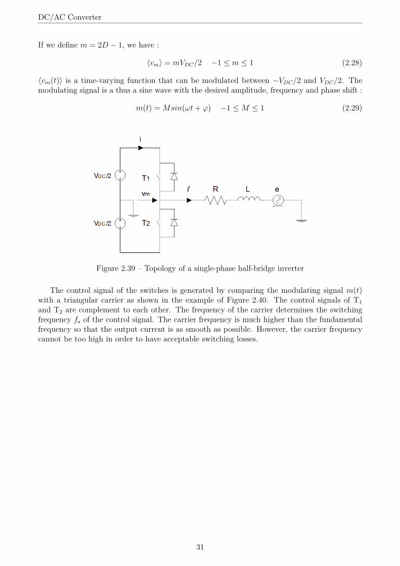
Figure 2.39 shows the simplest version of the single-phase inverter : it is a half-bridge voltagesource inverter (VSI) which contains two controllable switches.Like in the DC/DC converter, those switches can be MOSFETs or IGBTs depending on therequired breakdown voltages, power and switching frequency (Figure 2.15). IGBTs are preferredfor applications with output power higher than 5kW [37]. The antiparallel diodes can conductthe inductor current when all the switches are off. They can also conduct reverse current in thecase of unidirectional switches such as IGBTs. With this structure, the converter is bidirectionaland can thus also work as an AC/DC rectifier.The modulation technique used is called pulse-width modulation (PWM) : the pulse-width ofthe signal controlling the switches is modulated in order to control the average value of vm overone switching period. A 2-level PWM technique is used such that that vm is either high or low:
vm(t) =
+VDC/2 if T1 on and T2 off−VDC/2 if T1 off and T2 on
(2.25)
Considering one switching period Ts starting at t=0 is considered, we have :
vm(t) = VDC/2 0 ≤ t ≤ DTs
vm(t) = −VDC/2 DTs < t ≤ Ts(2.26)
where D is the duty cycle of the control signal. The average value of vm over one switchingperiod is thus :
〈vm〉 = DVDC/2− (1−D)VDC/2 0 ≤ D ≤ 1 (2.27)
30
DC/AC Converter
If we define m = 2D − 1, we have :
〈vm〉 = mVDC/2 −1 ≤ m ≤ 1 (2.28)
〈vm(t)〉 is a time-varying function that can be modulated between −VDC/2 and VDC/2. Themodulating signal is a thus a sine wave with the desired amplitude, frequency and phase shift :
m(t) = Msin(ωt+ ϕ) −1 ≤M ≤ 1 (2.29)
Figure 2.39 – Topology of a single-phase half-bridge inverter
The control signal of the switches is generated by comparing the modulating signal m(t)with a triangular carrier as shown in the example of Figure 2.40. The control signals of T1and T2 are complement to each other. The frequency of the carrier determines the switchingfrequency fs of the control signal. The carrier frequency is much higher than the fundamentalfrequency so that the output current is as smooth as possible. However, the carrier frequencycannot be too high in order to have acceptable switching losses.
31

DC/AC Converter
0 0.002 0.004 0.006 0.008 0.01 0.012 0.014 0.016 0.018 0.02-1
-0.5
0
0.5
1
m(t)
carrier
time[s]
0 0.002 0.004 0.006 0.008 0.01 0.012 0.014 0.016 0.018 0.020
0.5
1
control
signal
Figure 2.40 – Example of modulating signal (M = 0.8, ω = 2π50 rad/s), carrier (fs = 1kHz)and control signal for 2-level PWM
Based on the values of R and L, the output average current 〈i′(t)〉 can be computed withphasor equations :
I ′ = V m − EZ
(2.30)
with〈i′(t)〉 = I ′sin(ωt+ ψ) = =I ′ejωt (2.31)
e(t) = Esin(ωt) = =Eejωt (2.32)
〈vm(t)〉 = Vmsin(ωt+ ϕ) = =V mejωt (2.33)
Z = R + jωL (2.34)
Regardind the input average current 〈i(t)〉, power conservation gives
VDC〈i(t)〉 = 〈vm(t)〉〈i′(t)〉 (2.35)
which implies :
〈i(t)〉 = VmI′
VDC
sin(ωt+ ϕ)sin(ωt+ ψ) = VmI′
2VDC
(cos(ϕ− ψ)− cos(2ωt+ ϕ+ ψ)) (2.36)
The average input current of a single-phase inverter thus has a DC component as well as anAC component of angular frequency 2ω.
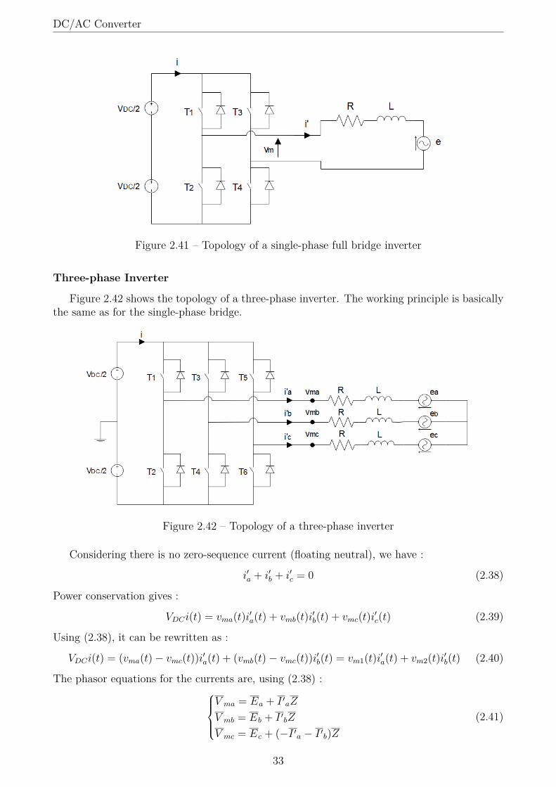
Another topology that can be used is the full bridge single-phase inverter as shown in Fig-ure 2.41. The working principle is exactly the same as for the half-bridge inverter except thatthe modulated voltage can vary between −VDC and VDC . In fact, we have :
vm(t) =
+VDC if T1, T4 on and T2, T3 off−VDC if T2, T3 on and T1, T4 off
(2.37)
32
DC/AC Converter
Figure 2.41 – Topology of a single-phase full bridge inverter
Three-phase Inverter
Figure 2.42 shows the topology of a three-phase inverter. The working principle is basicallythe same as for the single-phase bridge.
Figure 2.42 – Topology of a three-phase inverter
Considering there is no zero-sequence current (floating neutral), we have :
i′a + i′b + i′c = 0 (2.38)
Power conservation gives :
VDCi(t) = vma(t)i′a(t) + vmb(t)i′b(t) + vmc(t)i′c(t) (2.39)
Using (2.38), it can be rewritten as :
VDCi(t) = (vma(t)− vmc(t))i′a(t) + (vmb(t)− vmc(t))i′b(t) = vm1(t)i′a(t) + vm2(t)i′b(t) (2.40)
The phasor equations for the currents are, using (2.38) :V ma = Ea + I ′aZ
V mb = Eb + I ′bZ
V mc = Ec + (−I ′a − I ′b)Z(2.41)
33
DC/AC Converter
Substracting the third equations to the first and second, we have :V m1 = Eac + (2I ′a + I ′b)ZV m2 = Ebc + (2I ′b + I ′a)Z
(2.42)
These equations can be rewritten to isolate the currents :I ′a = (2V m1−V m2)−(2Eac−Ebc)3Z
I ′b = (2V m2−V m1)−(2Ebc−Eac)3Z
(2.43)
The system can thus be entirely described with two line voltages and currents.With this three-phase inverter topology, the modulated phase voltage can vary between−VDC/2and VDC/2. Hence, considering the modulated voltages are balanced, we have :
〈vma(t)〉 = ma(t)VDC/2 = Vmsin(ωt+ ϕ) (2.44)
〈vmb(t)〉 = mb(t)VDC/2 = Vmsin(ωt− 2π/3 + ϕ) (2.45)〈vmc(t)〉 = mc(t)VDC/2 = Vmsin(ωt− 4π/3 + ϕ) (2.46)
withVm ≤ VDC/2 (2.47)
Unlike for the single-phase inverter, 〈i(t)〉 has no component of angular frequency 2ω, if thesystem is balanced. The mathematical proof is given in Appendix A. However, 〈i(t)〉 has a 2ωcomponent if the system is unbalanced (negative sequence) [41].
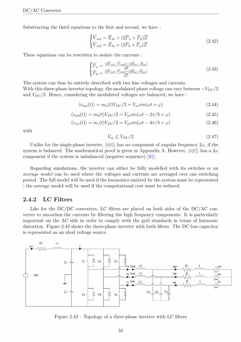
Regarding simulations, the inverter can either be fully modelled with its switches or anaverage model can be used where the voltages and currents are averaged over one switchingperiod. The full model will be used if the harmonics emitted by the system must be represented; the average model will be used if the computational cost must be reduced.
2.4.2 LC FiltersLike for the DC/DC converters, LC filters are placed on both sides of the DC/AC con-
verter to smoothen the currents by filtering the high frequency components. It is particularlyimportant on the AC side in order to comply with the grid standards in terms of harmonicdistortion. Figure 2.43 shows the three-phase inverter with both filters. The DC bus capacitoris represented as an ideal voltage source.
Figure 2.43 – Topology of a three-phase inverter with LC filters
34
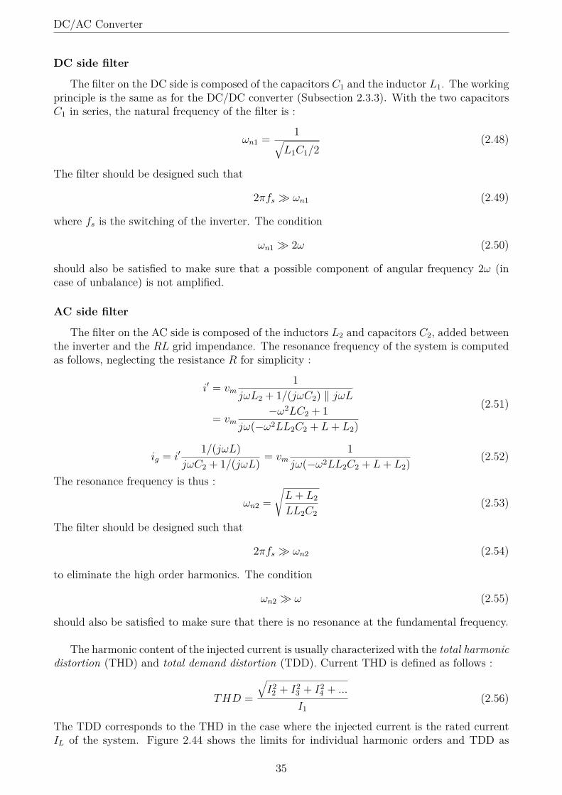
DC/AC Converter
DC side filter
The filter on the DC side is composed of the capacitors C1 and the inductor L1. The workingprinciple is the same as for the DC/DC converter (Subsection 2.3.3). With the two capacitorsC1 in series, the natural frequency of the filter is :
ωn1 = 1√L1C1/2
(2.48)
The filter should be designed such that
2πfs ωn1 (2.49)
where fs is the switching of the inverter. The condition
ωn1 2ω (2.50)
should also be satisfied to make sure that a possible component of angular frequency 2ω (incase of unbalance) is not amplified.
AC side filter
The filter on the AC side is composed of the inductors L2 and capacitors C2, added betweenthe inverter and the RL grid impendance. The resonance frequency of the system is computedas follows, neglecting the resistance R for simplicity :
i′ = vm1
jωL2 + 1/(jωC2) ‖ jωL
= vm−ω2LC2 + 1
jω(−ω2LL2C2 + L+ L2)
(2.51)
ig = i′1/(jωL)
jωC2 + 1/(jωL) = vm1
jω(−ω2LL2C2 + L+ L2)(2.52)
The resonance frequency is thus :
ωn2 =√L+ L2
LL2C2(2.53)
The filter should be designed such that
2πfs ωn2 (2.54)
to eliminate the high order harmonics. The condition
ωn2 ω (2.55)
should also be satisfied to make sure that there is no resonance at the fundamental frequency.
The harmonic content of the injected current is usually characterized with the total harmonicdistortion (THD) and total demand distortion (TDD). Current THD is defined as follows :
THD =
√I2
2 + I23 + I2
4 + ...
I1(2.56)
The TDD corresponds to the THD in the case where the injected current is the rated currentIL of the system. Figure 2.44 shows the limits for individual harmonic orders and TDD as
35
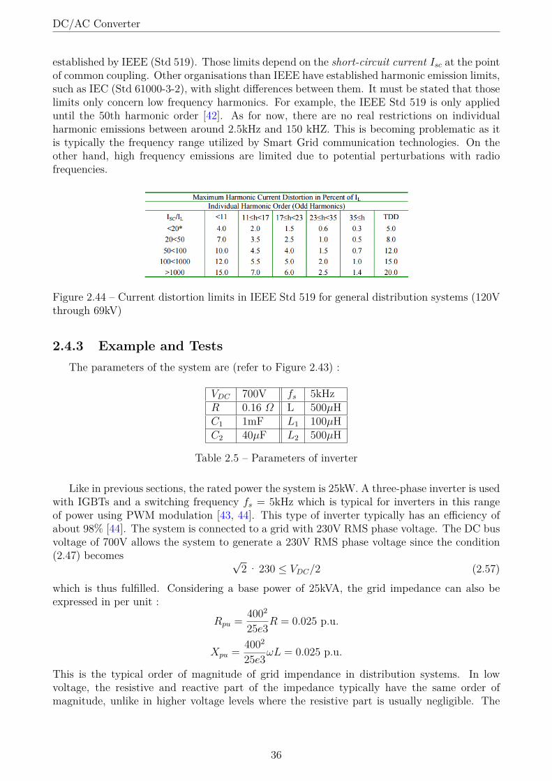
DC/AC Converter
established by IEEE (Std 519). Those limits depend on the short-circuit current Isc at the pointof common coupling. Other organisations than IEEE have established harmonic emission limits,such as IEC (Std 61000-3-2), with slight differences between them. It must be stated that thoselimits only concern low frequency harmonics. For example, the IEEE Std 519 is only applieduntil the 50th harmonic order [42]. As for now, there are no real restrictions on individualharmonic emissions between around 2.5kHz and 150 kHZ. This is becoming problematic as itis typically the frequency range utilized by Smart Grid communication technologies. On theother hand, high frequency emissions are limited due to potential perturbations with radiofrequencies.
Figure 2.44 – Current distortion limits in IEEE Std 519 for general distribution systems (120Vthrough 69kV)
2.4.3 Example and TestsThe parameters of the system are (refer to Figure 2.43) :
VDC 700V fs 5kHzR 0.16 Ω L 500µHC1 1mF L1 100µHC2 40µF L2 500µH
Table 2.5 – Parameters of inverter
Like in previous sections, the rated power the system is 25kW. A three-phase inverter is usedwith IGBTs and a switching frequency fs = 5kHz which is typical for inverters in this rangeof power using PWM modulation [43, 44]. This type of inverter typically has an efficiency ofabout 98% [44]. The system is connected to a grid with 230V RMS phase voltage. The DC busvoltage of 700V allows the system to generate a 230V RMS phase voltage since the condition(2.47) becomes √
2 · 230 ≤ VDC/2 (2.57)
which is thus fulfilled. Considering a base power of 25kVA, the grid impedance can also beexpressed in per unit :
Rpu = 4002
25e3R = 0.025 p.u.
Xpu = 4002
25e3ωL = 0.025 p.u.
This is the typical order of magnitude of grid impendance in distribution systems. In lowvoltage, the resistive and reactive part of the impedance typically have the same order ofmagnitude, unlike in higher voltage levels where the resistive part is usually negligible. The
36
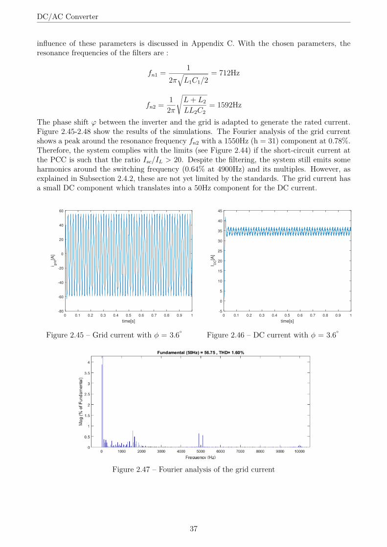
DC/AC Converter
influence of these parameters is discussed in Appendix C. With the chosen parameters, theresonance frequencies of the filters are :
fn1 = 12π
√L1C1/2
= 712Hz
fn2 = 12π
√L+ L2
LL2C2= 1592Hz
The phase shift ϕ between the inverter and the grid is adapted to generate the rated current.Figure 2.45-2.48 show the results of the simulations. The Fourier analysis of the grid currentshows a peak around the resonance frequency fn2 with a 1550Hz (h = 31) component at 0.78%.Therefore, the system complies with the limits (see Figure 2.44) if the short-circuit current atthe PCC is such that the ratio Isc/IL > 20. Despite the filtering, the system still emits someharmonics around the switching frequency (0.64% at 4900Hz) and its multiples. However, asexplained in Subsection 2.4.2, these are not yet limited by the standards. The grid current hasa small DC component which translates into a 50Hz component for the DC current.
time[s]
0 0.1 0.2 0.3 0.4 0.5 0.6 0.7 0.8 0.9 1
i grid[A
]
-80
-60
-40
-20
0
20
40
60
Figure 2.45 – Grid current with φ = 3.6
time[s]
0 0.1 0.2 0.3 0.4 0.5 0.6 0.7 0.8 0.9 1
I DC[A
]
-5
0
5
10
15
20
25
30
35
40
45
Figure 2.46 – DC current with φ = 3.6
Figure 2.47 – Fourier analysis of the grid current
37

Grid-side Controller
Figure 2.48 – Fourier analysis of the DC current
2.5 Grid-side Controller
2.5.1 General StructureThe grid-side controller is in charge of• Balancing the system in terms of active power by regulating the DC bus voltage.• Controlling the reactive power injection.• Controlling the current injected to/from the grid and making sure the current is sub-
stantially balanced and harmonic-free. This particularly important in a microgrid en-vironment where the power qualtiy perturbations can be problematic in island mode.This control requires some sort of synchronization with the grid.
• Generating the modulating signals for the PWM inverter.Figure 2.49 shows an example of grid-side controller structure. The syncronous reference framecontrol, also called dq control, uses a reference frame transformation, abc → dq, to transformthe grid current and voltage waveforms into a reference frame that rotates synchronously withthe grid voltage. By means of this, the control variables become DC values; thus, filteringand controlling can be easier achieved. The dq control structure is normally associated withproportional–integral (PI) controllers since they have a satisfactory behavior when regulatingDC variables. To improve the performance of PI controller in such a structure, cross-couplingterms and voltage feedforward are usually used [45].
A synchronization system is required to synchronize the grid currents with the grid volt-age. A very common synchronization technique is the phase-locked loop (PLL) system. It isdescribed in details in subsection 2.5.2. The PLL measures the phase θ of the voltage vectorwhich is then used, in the case of dq control structure, to operate the abc → dq transforma-tions. The PLL is also used to measure the grid frequency. The DC link (active power) and Q(reactive power) controllers generate the reference currents in the dq frame.
38
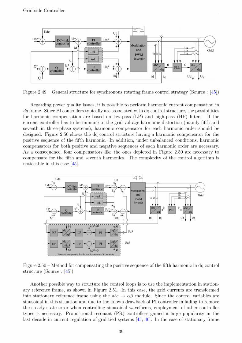
Grid-side Controller
Figure 2.49 – General structure for synchronous rotating frame control strategy (Source : [45])
Regarding power quality issues, it is possible to perform harmonic current compensation indq frame. Since PI controllers typically are associated with dq control structure, the possibilitiesfor harmonic compensation are based on low-pass (LP) and high-pass (HP) filters. If thecurrent controller has to be immune to the grid voltage harmonic distortion (mainly fifth andseventh in three-phase systems), harmonic compensator for each harmonic order should bedesigned. Figure 2.50 shows the dq control structure having a harmonic compensator for thepositive sequence of the fifth harmonic. In addition, under unbalanced conditions, harmoniccompensators for both positive and negative sequences of each harmonic order are necessary.As a consequence, four compensators like the ones depicted in Figure 2.50 are necessary tocompensate for the fifth and seventh harmonics. The complexity of the control algorithm isnoticeable in this case [45].
Figure 2.50 – Method for compensating the positive sequence of the fifth harmonic in dq controlstructure (Source : [45])
Another possible way to structure the control loops is to use the implementation in station-ary reference frame, as shown in Figure 2.51. In this case, the grid currents are transformedinto stationary reference frame using the abc → αβ module. Since the control variables aresinusoidal in this situation and due to the known drawback of PI controller in failing to removethe steady-state error when controlling sinusoidal waveforms, employment of other controllertypes is necessary. Proportional resonant (PR) controllers gained a large popularity in thelast decade in current regulation of grid-tied systems [45, 46]. In the case of stationary frame
39

Grid-side Controller
control, cross-coupling terms and voltage feedforward are not necessary. Voltage feedforwardis used here nonetheless, as it provides soft-start capabilities [41]. The PLL is also necessaryto operate dq → αβ transformation for the reference currents.
Characteristic to this controller is the fact that it achieves a very high gain around the reso-nance frequency, thus being capable to eliminate the steady-state error between the controlledsignal and its reference. Moreover, high dynamic characteristics of PR controller have beenreported in different works [45, 46].
Regarding harmonic compensation, things are different than in synchrounous frame control.Several harmonic compensators (HC) are cascaded and tuned at the desired frequency. In thisway, selective harmonic compensation at different frequencies is obtained. Only one block isrequired to control both positive and negative sequences for each harmonic. The resultingstructure is shown in Figure 2.52. The structure is noticeably simpler than for synchronousframe control. For all these reasons, stationary frame control with PR controllers is chosen herefor the BESS.
Figure 2.51 – General structure for stationary reference frame control strategy (Source : [45])
Figure 2.52 – Structure of the harmonic compensator attached to the resonant controller of thefundamental current (Source : [45])
2.5.2 Phase-locked LoopThe role of the PLL is to measure the phase and frequency of the grid voltage. Two types
of PLL are presented and compared here : the synchronous reference frame PLL (SRF-PLL)and the enhanced PLL (EPLL).
40

Grid-side Controller
SRF-PLL
The SRF-PLL is arguably the most well-known and widely used concept in the general areasof power engineering [47]. Its structure is depicted in Figure 2.53.
Figure 2.53 – Three-phase SRF-PLL structure (Source : [47])
The PI controller brings the error signal uq to zero in steady-state. The estimated phase andangular frequency are respectively φ0 and ω0. The abc → dq0 Park transformation is definedby udq0 = Puabc where
P = 23
sinφ0 sin(φ0 − 2π/3) sin(φ0 − 4π/3)cosφ0 cos(φ0 − 2π/3) cos(φ0 − 4π/3)1/2 1/2 1/2
(2.58)
The drawback of the SRF-PLL is that the phase and frequency estimations are perturbedwhen the grid voltage is polluted with harmonics or unbalanced. Moreover, there is a trade-offat the PI controller between
• a fast controller that reacts quickly to phase/frequency changes but that is vulnerableto grid perturbations.
• a controller that is robust towards perturbations but has a slow response time.In Figures 2.54-2.57, the grid voltage (400V line RMS) subsequently undergoes a frequencyjump, phase jump and 5th harmonic injection with different values of PI parameters h1 andh2. The harmonic injection induces an oscillating signal, both for the frequency and phaseestimation. It is not shown here but in case of unbalance, an oscillating signal of angularfrequency 2ω appears. The influence of the paremeters is as follows :
• In terms of frequency, increasing h1 improves the response time but increases the errorin case of phase jump and amplifies the oscillations due to harmonics. h1 doesn’t havemuch of an influence on phase estimation.
• In terms of frequency, increasing h2 deteriorates the response time but decreases theerror in case of phase jump. In terms of phase error, increasing h2 makes the PLLrecover faster from a phase jump but amplifies the oscillations due to harmonics.
41

Grid-side Controller
time[s]
0 0.05 0.1 0.15 0.2 0.25 0.3 0.35 0.4
f est[H
z]
50
50.5
51
51.5
52
52.5
53
53.5
54
54.5
h1 = 100
h1 = 200
Figure 2.54 – Frequency estimation with1Hz frequency jump at t=0.1s, 15 phasejump at t=0.2s and 5% of 5th harmonicinjection at t=0.3s, h2 = 2
time[s]
0 0.05 0.1 0.15 0.2 0.25 0.3 0.35 0.4
φ -
φe
st[d
eg]
-2
0
2
4
6
8
10
12
14
16
h1 = 100
h1 = 200
Figure 2.55 – Phase error with 1Hz fre-quency jump at t=0.1s, 15 phase jump att=0.2s and 5% of 5th harmonic injection att=0.3s, h2 = 2
time[s]
0 0.05 0.1 0.15 0.2 0.25 0.3 0.35 0.4
f est[H
z]
50
50.5
51
51.5
52
52.5
53
h2 = 2
h2 = 4
Figure 2.56 – Frequency estimation with1Hz frequency jump at t=0.1s, 15 phasejump at t=0.2s and 5% of 5th harmonicinjection at t=0.3s, h1 = 100
time[s]
0 0.05 0.1 0.15 0.2 0.25 0.3 0.35 0.4
φ -
φe
st[d
eg]
-4
-2
0
2
4
6
8
10
12
14
16
h2 = 2
h2 = 4
Figure 2.57 – Phase error with 1Hz fre-quency jump at t=0.1s, 15 phase jump att=0.2s and 5% of 5th harmonic injection att=0.3s, h1 = 100
EPLL
Figure 2.58 shows the structure of the three-phase EPLL where ( · ) is the dot product oftwo vectors and
C(φ0) =
cosφ0cos(φ0 − 2π/3)cos(φ0 − 4π/3)
S(φ0) =
sinφ0sin(φ0 − 2π/3)sin(φ0 − 4π/3)
(2.59)
42

Grid-side Controller
Figure 2.58 – Three-phase EPLL structure (Source : [47])
The EPLL is an extension of the SRF-PLL with an additional loop that estimates theamplitude U0 of the signal. In this way, the EPLL provides an estimation of the whole signalyabc while the SRF-PLL only estimates the phase and frequency. With this structure, theEPLL can be further extended, for example with an estimation of the negative sequence of thefundamental component of the signal, as depicted in Figure 2.59.
Figure 2.59 – Three-phase EPLL structure with positive and negative sequence estimation(Source : [47])
V0, ψ0, zabc are respectively the estimated amplitude, phase and signal of the negativesequence. The negative sequence block uses the frequency estimation provided by the positivesequence block. With this structure, the negative sequence is exctracted, hence the phase φ0
43

Grid-side Controller
and frequency ω0 estimations are not affected by an unbalance. The EPLL can even be furtherextended to extract positive and negative sequence of harmonics, as shown in Figure 2.60. Thechoice made here is to extract the 5th and 7th harmonics.
Figure 2.60 – Extendend EPLL to estimate the harmonic of order k (Source : [47])
From now on, the values of the parameters of the EPLL (referred to Figure 2.59) are :
µ1 200 µ2 100µ3 2 µ4 200µ5 2
Table 2.6 – Parameters of EPLL
The values of the parameters are the same for the harmonics blocks (µ4 and µ5). In Figures2.61-2.64, the grid voltage subsequently undergoes a frequency jump, phase jump, 5th and 7thharmonic injection and 1-phase voltage dip. The voltage dip induces a negative sequence atthe fundamental frequency. It can be observed that EPLL filters rather quickly the effects ofthe harmonics and unbalance, while being able to track frequency and phase jumps. For thesereasons, the EPLL is the chosen synchronization system for the BESS. Post-filtering of thefrequency estimation can also be used if necessary.
44

Grid-side Controller
time[s]
0 0.1 0.2 0.3 0.4 0.5 0.6
f est[H
z]
49.5
50
50.5
51
51.5
52
52.5
53
53.5
Figure 2.61 – Frequency estimation with1Hz frequency jump at t=0.1s, 15 phasejump at t=0.2s, 5% of 5th and 3% of 7thharmonic injection at t=0.3s, 50% 1-phasevoltage dip from t=0.4s to t=0.5s
time[s]
0 0.1 0.2 0.3 0.4 0.5 0.6
φ -
φe
st[d
eg]
-10
-5
0
5
10
15
20
Figure 2.62 – Phase error with 1Hz fre-quency jump at t=0.1s, 15 phase jump att=0.2s, 5% of 5th and 3% of 7th harmonicinjection at t=0.3s, 50% 1-phase voltagedip from t=0.4s to t=0.5s
time[s]
0 0.1 0.2 0.3 0.4 0.5 0.6
Am
plit
ude
est[V
]
-50
0
50
100
150
200
250
300
350
VP1
VN1
Figure 2.63 – Amplitude estimation of fun-damental postive and negative sequencewith 1Hz frequency jump at t=0.1s, 15
phase jump at t=0.2s, 5% of 5th and 3%of 7th harmonic injection at t=0.3s, 50%1-phase voltage dip from t=0.4s to t=0.5s
time[s]
0 0.1 0.2 0.3 0.4 0.5 0.6
Am
plit
ude
est[V
]
-10
-5
0
5
10
15
20
25
30
35
40
VP5
VP7
Figure 2.64 – Amplitude estimation of 5thand 7th harmonics (positive sequence) with1Hz frequency jump at t=0.1s, 15 phasejump at t=0.2s, 5% of 5th and 3% of 7thharmonic injection at t=0.3s, 50% 1-phasevoltage dip from t=0.4s to t=0.5s
2.5.3 PR ControllersThe general transfer function a PR controller is the following :
C(s) = KP + 2ωcKIs
s2 + 2ωcs+ ω2n
(2.60)
The term in ωc at the denominator is a necessary damping term to make sure the gain is notinfinite at the natural frequency, othwerise causing instability. ωc corresponds to the cutofffrequency, which means that the gain at ωn ± ωc is 3dB smaller than at ωn. Figures 2.65 and
45

Grid-side Controller
2.66 show the influence of KI and ωc. Increasing KI raises the gain at the natural frequency butleads to a wider band. Increasing ωc does not change the gain at the natural frequency and leadsto a wider band. The proportional term KP helps the controller with soft-start capabilities. Itshould be noted that the PR controller uses the estimation of the PLL as natural frequencyto make sure it keeps working even when the grid frequency changes. Stability problems canarise if the PR parameters are not chosen carefully. In fact, if the gain of the controller atthe resonance frequency of the output LC filter is too high, the system will go into resonance.All the parameters of the PR controller thus have to be chosen carefully, taking into accountthe values of the inductance and capacitance of the LC filter. Considering H(s) is the transferfunction between the input signal of the LC filter vm and and the ouput signal ig, the followingresult can be obtained (refer to Figure 2.43) :
H(s) = igvm
= 1/(LL2C2)s3 + s2R/L+ s(L+ L2)/(LL2C2) +R/(LL2C2)
(2.61)
The open-loop gain of the fundamental current is then C(s)H(s) and the stability of the systemdepends on the closed-loop transfer function (unity feedback) which is
Tr(s) = C(s)H(s)1 + C(s)H(s) (2.62)
Specifically, the real part of each pole of Tr(s) must be negative to ensure stability. Gain andphase margins are also commonly used to determine how close the system is to instability. Theclosed-loop system is unstable if the open-loop gain is greater than 1 at the frequency f180 atwhich the phase is 180 . From there, they are defined as follows :
• The gain margin is the difference between the open-loop gain at f180 and unity gain (0dB). It also corresponds to the possible increase in feedback gain before the closed-loopsystem becomes unstable.
• The phase margin is the difference between 180 and the phase at which the gain is 0dB.
Additional resonant controllers are used in parallel for the 5th and 7th harmonic currents. Thetransfer function of those controllers is :
Ck(s) = 2ωcKIs
s2 + 2ωcs+ (kωn)2 k = 5, 7 (2.63)
The reference current is balanced, hence the setpoints of the harmonic and unbalanced cur-rents are zero. Some active compensation techniques consist in intentionally injecting un-balanced/harmonic current in order to decrease the unbalance/harmonic content of the PCCvoltage. This is thus not considered here. The output of the current controller is the referencevoltage vector in αβ frame. This vector is then transformed into the modulating signals for theinverter.
46
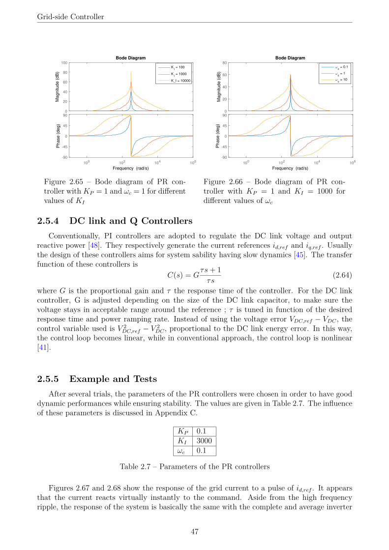
Grid-side Controller
Mag
nitude
(dB
)
0
20
40
60
80
100
100 102 104 106
Pha
se (
deg)
-90
-45
0
45
90
KI = 100
KI = 1000
K_I = 10000
Bode Diagram
Frequency (rad/s)
Figure 2.65 – Bode diagram of PR con-troller withKP = 1 and ωc = 1 for differentvalues of KI
Mag
nitude
(dB
)
0
20
40
60
80
100 102 104 106
Pha
se (
deg)
-90
-45
0
45
90
ωc = 0.1
ωc = 1
ωc = 10
Bode Diagram
Frequency (rad/s)
Figure 2.66 – Bode diagram of PR con-troller with KP = 1 and KI = 1000 fordifferent values of ωc
2.5.4 DC link and Q ControllersConventionally, PI controllers are adopted to regulate the DC link voltage and output
reactive power [48]. They respectively generate the current references id,ref and iq,ref . Usuallythe design of these controllers aims for system sability having slow dynamics [45]. The transferfunction of these controllers is
C(s) = Gτs+ 1τs
(2.64)
where G is the proportional gain and τ the response time of the controller. For the DC linkcontroller, G is adjusted depending on the size of the DC link capacitor, to make sure thevoltage stays in acceptable range around the reference ; τ is tuned in function of the desiredresponse time and power ramping rate. Instead of using the voltage error VDC,ref − VDC , thecontrol variable used is V 2
DC,ref − V 2DC , proportional to the DC link energy error. In this way,
the control loop becomes linear, while in conventional approach, the control loop is nonlinear[41].
2.5.5 Example and TestsAfter several trials, the parameters of the PR controllers were chosen in order to have good
dynamic performances while ensuring stability. The values are given in Table 2.7. The influenceof these parameters is discussed in Appendix C.
KP 0.1KI 3000ωc 0.1
Table 2.7 – Parameters of the PR controllers
Figures 2.67 and 2.68 show the response of the grid current to a pulse of id,ref . It appearsthat the current reacts virtually instantly to the command. Aside from the high frequencyripple, the response of the system is basically the same with the complete and average inverter
47

Grid-side Controller
models.The zero-pole map of the closed-loop current controller is depicted in Figures 2.69 and 2.70. Asthe real part of each pole of the system is negative, the system is stable. The gain and phasemargins of the system are given in Figure 2.71. The stability performances can be enhanced byusing semi-state feedback(s), for instance with the current of the filtering inductance and/orthe voltage of the filtering capacitor [41]. This is not considered here.The DC link and Q controllers are tested with the whole system in Section 2.6.
time[s]
0 0.05 0.1 0.15 0.2 0.25 0.3 0.35 0.4
i res1[A
]
-80
-60
-40
-20
0
20
40
60
Figure 2.67 – Grid current ires1 with a pulseof id,ref from t=0.1s to t=0.3s, using com-plete inverter model
time[s]
0 0.05 0.1 0.15 0.2 0.25 0.3 0.35 0.4
i res1[A
]
-60
-40
-20
0
20
40
60
Figure 2.68 – Grid current ires1 with a pulseof id,ref from t=0.1s to t=0.3s, using aver-age inverter model
-6000 -5000 -4000 -3000 -2000 -1000 0
×104
-1
-0.8
-0.6
-0.4
-0.2
0
0.2
0.4
0.6
0.8
1
Pole-Zero Map
Real Axis (seconds-1)
Imagin
ary
Axis
(se
cond
s-1
)
Figure 2.69 – Pole-zero map of closed-loopcurrent controller (red : zoom)
-400 -300 -200 -100 0 100 200 300 400
-8000
-6000
-4000
-2000
0
2000
4000
6000
8000
10000
Pole-Zero Map
Real Axis (seconds-1)
Imagin
ary
Axis
(se
cond
s-1
)
Figure 2.70 – Zoom of pole-zero map ofclosed-loop current controller
48

Tests on Complete BESS
Magnitude (
dB
)-150
-100
-50
0
50
100
100 101 102 103 104 105 106
Phase (
deg)
-360
-270
-180
-90
0
90
Bode Diagram
Gm = 3.92 dB (at 9.95e+03 rad/s) , Pm = 17.6 deg (at 835 rad/s)
Frequency (rad/s)
Figure 2.71 – Bode diagram of the open-loop gain and phase/gain margins of the closed-loopsystem
2.6 Tests on Complete BESSTwo tests are executed on the complete BESS. Tne first one shows how the system behaves
when the grid undergoes perturbations such as harmonics and voltage dip. The goal is thus toevaluate the power quality provided by the BESS as well as the fault-ride through capability.The second test evaluates the ability of the system of to follow a series of active and reactivepower setpoints. The average dynamic model is chosen for the DC/DC converter but thecomplete model is used for the inverter in order to evaluate the harmonic content of the gridcurrent. The value chosen for the DC link capacitor is CDC = 4mF. The equation for the DClink voltage is
VDC =∫
(IDAB − IDC,inv)/CDC dt (2.65)
where IDAB is the current from the DAB converter and IDC,inv is the DC current to the inverter.The parameters of the DC link and Q controllers are given in Table 2.8. The influence of theseparemeters is discussed in Appendix D.
DC link QG 1e-3 [A/V2] 2.5e-3 [A/VAr]τ 100ms 20ms
Table 2.8 – Parameters of DC link and Q controllers
2.6.1 Power Quality and Fault-ride Through CapabilityThe test is the follwowing : a step of power setpoint is sent to the battery, then the grid
undergoes a 1-phase voltage dip and finally 5th and 7th harmonics are added to the grid voltage.The results are depicted in Figures 2.72-2.78.The output active power does not show much perturbations due to voltage dip or harmonics.The unbalance due to the 1-phase voltage dip induces a 2ω component in the DC inverter whichconsequently appears in the DC link voltage. During the voltage dip, the voltage setpoint allowsto keep the grid current balanced. Equally, after the addition of harmonics, the voltage setpoint
49

Tests on Complete BESS
is adapted to control the grid current harmonics.The comparison of the harmonic limits in Figure 2.44 with the Fourier analysis in Figure 2.78(0.98% at 1600Hz) shows that the grid current complies with the standard if Isc/IL > 20 atthe PCC. Figure 2.77 shows that the DC current of the inverter, despite the LC filter, has a lotof high frequency ripple. Hence, the DC link capacitance must be large enough to effectivelyfilter this ripple.
time[s]
0 0.1 0.2 0.3 0.4 0.5 0.6 0.7 0.8 0.9 1
Pre
s[k
W]
& Q
res[k
VA
r]
-5
0
5
10
15
20
25
30
Pres
Qres
Figure 2.72 – Active and reactive power(positive fundamental sequence) injectedto the grid with 25kW setpoint step att=0.1s, 50% 1-phase voltage dip fromt=0.3s to t=0.5s, addition of 5% of 5th har-monic and 3% of 7th harmonic from t=0.6s
time[s]
0 0.1 0.2 0.3 0.4 0.5 0.6 0.7 0.8 0.9 1
Vb
usD
C[V
]
690
695
700
705
710
715
720
725
730
735
Figure 2.73 – DC link voltage with 25kWsetpoint step at t=0.1s, 50% 1-phase volt-age dip from t=0.3s to t=0.5s, addition of5% of 5th harmonic and 3% of 7th har-monic from t=0.6s
time[s]
0 0.1 0.2 0.3 0.4 0.5 0.6 0.7 0.8 0.9 1
i res1, i re
s2[A
]
-80
-60
-40
-20
0
20
40
60
80
ires1
ires2
Figure 2.74 – Grid currents with 25kW set-point step at t=0.1s, 50% 1-phase voltagedip from t=0.3s to t=0.5s, addition of 5%of 5th harmonic and 3% of 7th harmonicfrom t=0.6s
time[s]
0 0.1 0.2 0.3 0.4 0.5 0.6 0.7 0.8 0.9 1
um
1,r
ef,
um
2,r
ef[V
]
-800
-600
-400
-200
0
200
400
600
800u
m1,ref
um2,ref
Figure 2.75 – Reference line voltages (out-put of PR) with 25kW setpoint step att=0.1s, 50% 1-phase voltage dip fromt=0.3s to t=0.5s, addition of 5% of 5th har-monic and 3% of 7th harmonic from t=0.6s
50

Tests on Complete BESS
time[s]
0 0.1 0.2 0.3 0.4 0.5 0.6 0.7 0.8 0.9 1
I DA
B[A
]
-5
0
5
10
15
20
25
30
35
40
Figure 2.76 – Output current of DAB con-verter with 25kW setpoint step at t=0.1s,50% 1-phase voltage dip from t=0.3s tot=0.5s, addition of 5% of 5th harmonic and3% of 7th harmonic from t=0.6s
0 0.1 0.2 0.3 0.4 0.5 0.6 0.7 0.8 0.9 1
I DC
,in
v[A
]
-10
0
10
20
30
40
50
time[s]
Figure 2.77 – DC side inverter current with25kW setpoint step at t=0.1s, 50% 1-phasevoltage dip from t=0.3s to t=0.5s, additionof 5% of 5th harmonic and 3% of 7th har-monic from t=0.6s
Figure 2.78 – Fourier analysis of ires1 from t=0.7s to t=1s
2.6.2 Power Setpoints FollowingA series of ramps are given as reference for active and reactive power. Results are depicted
in Figures 2.79 and 2.80.They show that the BESS can follow a series of subsequent setpoints rather effectively and thatthe active and reactive powers can be controlled independently. The output power lags around20ms in average behind the command. The maximum power ramping rate achieved is about4ms/kW 3.
3. This corresponds to the typical ramping rate of the SAFT Li-ion battery used by Laborelec.
51

Tests on Complete BESS
time[s]
0 0.2 0.4 0.6 0.8 1 1.2
Active p
ow
er[
kW
] a
nd R
ea
ctive p
ow
er[
kV
Ar]
-30
-20
-10
0
10
20
30
P
Pref
Q
Qref
Figure 2.79 – Output active and reactivepowers (solid lines) after several setpointramps (dashed lines)
time[s]
0 0.2 0.4 0.6 0.8 1 1.2
Vb
usD
C[V
]
660
670
680
690
700
710
720
730
Figure 2.80 – DC link voltage after severalsetpoint ramps
52

Chapter 3
Applications of BESS in Microgrids
3.1 OverviewDue to the variability and intermittency of renewable distributed generators (DGs), the op-
eration and control of renewable microgrids is challenging. The weather-dependent DGs maynot be able to accommodate the constantly varying load very well and their fluctuation mayeven cause instability. Thus, ESS are very important in microgrids, especially for renewablemicrogrids. Since an ESS can operate as load or generator when it is in charging or dischargingmode, it is able to balance the power in the microgrid and reduce the impact of any fluctuation.This improves the stability of the microgrid significantly [6]. The general applications and con-figurations of ESS in microgrids are presented hereafter, BESS being one choice of technologyamong others. The suited application for an ESS depends on its energy capacity, power ratingand response time.
For different applications, the configuration of ESS may need to be different. There aretwo different configurations of ESS in a renewable microgrid : the aggregated ESS and dis-tributed ESS. The different structure determines their performance and applications.
An aggregated ESS is a big energy storage facility with dedicated housing in the microgrid.It has usually very large energy capacity and power capability. According to some research[49, 50], an aggregated ESS is more capable of suppressing the power fluctuation in the micro-grid than a distributed ESS. This is because the power output of the entire renewable farmis usually more stable than each individual unit (averaging effect). Besides fluctuation sup-pression, aggreggated ESS also perform energy management features, such as load leveling andpeak shifting [6].
There are two different configurations of distributed ESS. One is the distributed ESS ongenerator side which helps the DGs to smoothen output power. Another type is the distributedESS on load side which allows to reduce the load variation and manage energy for different pur-poses. Distributed ESS are smaller than aggreggated ESS because they only handle a single (ora small group) renewable generation unit or load. When used with a renewable generation unit,the distributed ESS is usually connected to the same DC link, behind the grid-side inverter.In this configuration, the ESS helps to have a stable DC link votlage by compensating thefluctuation of renewable generation. As mentioned before, a distributed ESS is not as powerfulas an aggregated ESS for mitigating the fluctuation of renewables, but the distributed ESS iseasier to be expanded and maintained [6].
An ESS is useful for managing energy and improving the stability and economy of a mi-
53
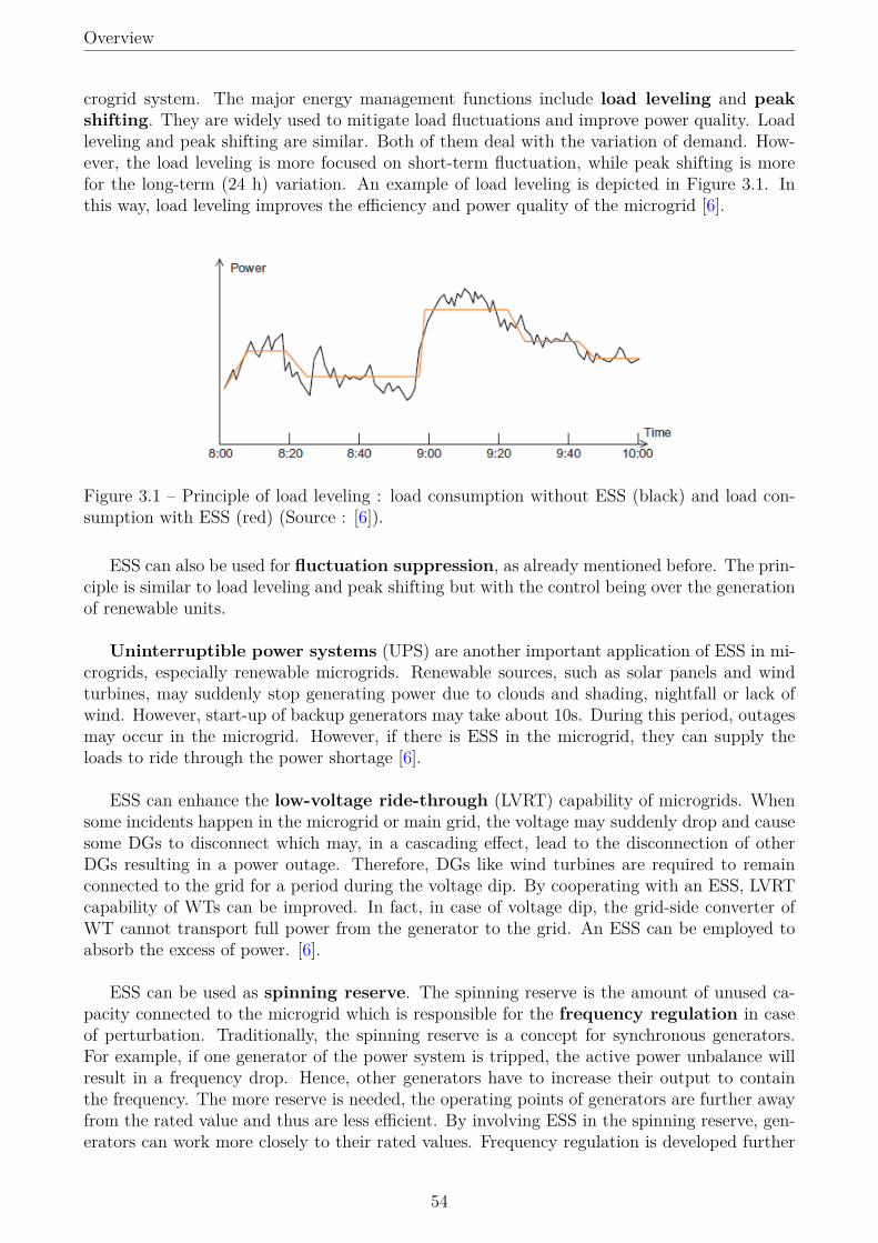
Overview
crogrid system. The major energy management functions include load leveling and peakshifting. They are widely used to mitigate load fluctuations and improve power quality. Loadleveling and peak shifting are similar. Both of them deal with the variation of demand. How-ever, the load leveling is more focused on short-term fluctuation, while peak shifting is morefor the long-term (24 h) variation. An example of load leveling is depicted in Figure 3.1. Inthis way, load leveling improves the efficiency and power quality of the microgrid [6].
Figure 3.1 – Principle of load leveling : load consumption without ESS (black) and load con-sumption with ESS (red) (Source : [6]).
ESS can also be used for fluctuation suppression, as already mentioned before. The prin-ciple is similar to load leveling and peak shifting but with the control being over the generationof renewable units.
Uninterruptible power systems (UPS) are another important application of ESS in mi-crogrids, especially renewable microgrids. Renewable sources, such as solar panels and windturbines, may suddenly stop generating power due to clouds and shading, nightfall or lack ofwind. However, start-up of backup generators may take about 10s. During this period, outagesmay occur in the microgrid. However, if there is ESS in the microgrid, they can supply theloads to ride through the power shortage [6].
ESS can enhance the low-voltage ride-through (LVRT) capability of microgrids. Whensome incidents happen in the microgrid or main grid, the voltage may suddenly drop and causesome DGs to disconnect which may, in a cascading effect, lead to the disconnection of otherDGs resulting in a power outage. Therefore, DGs like wind turbines are required to remainconnected to the grid for a period during the voltage dip. By cooperating with an ESS, LVRTcapability of WTs can be improved. In fact, in case of voltage dip, the grid-side converter ofWT cannot transport full power from the generator to the grid. An ESS can be employed toabsorb the excess of power. [6].
ESS can be used as spinning reserve. The spinning reserve is the amount of unused ca-pacity connected to the microgrid which is responsible for the frequency regulation in caseof perturbation. Traditionally, the spinning reserve is a concept for synchronous generators.For example, if one generator of the power system is tripped, the active power unbalance willresult in a frequency drop. Hence, other generators have to increase their output to containthe frequency. The more reserve is needed, the operating points of generators are further awayfrom the rated value and thus are less efficient. By involving ESS in the spinning reserve, gen-erators can work more closely to their rated values. Frequency regulation is developed further
54
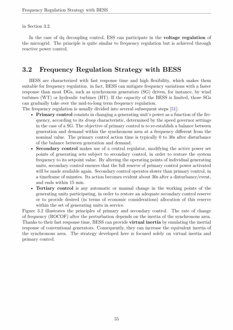
Frequency Regulation Strategy with BESS
in Section 3.2.
In the case of dq decoupling control, ESS can participate in the voltage regulation ofthe microgrid. The principle is quite similar to frequency regulation but is achieved throughreactive power control.
3.2 Frequency Regulation Strategy with BESSBESS are characterized with fast response time and high flexibility, which makes them
suitable for frequency regulation. in fact, BESS can mitigate frequency variations with a fasterresponse than most DGs, such as synchronous generators (SG) driven, for instance, by windturbines (WT) or hydraulic turbines (HT). If the capacity of the BESS is limited, those SGscan gradually take over the mid-to-long term frequency regulation.The frequency regulation is usually divided into several subsequent steps [51]:
• Primary control consists in changing a generating unit’s power as a function of the fre-quency, according to its droop characteristic, determined by the speed governor settingsin the case of a SG. The objective of primary control is to re-establish a balance betweengeneration and demand within the synchronous area at a frequency different from thenominal value. The primary control action time is typically 0 to 30s after disturbanceof the balance between generation and demand.
• Secondary control makes use of a central regulator, modifying the active power setpoints of generating sets subject to secondary control, in order to restore the systemfrequency to its setpoint value. By altering the operating points of individual generatingunits, secondary control ensures that the full reserve of primary control power activatedwill be made available again. Secondary control operates slower than primary control, ina timeframe of minutes. Its action becomes evident about 30s after a disturbance/event,and ends within 15 min.
• Tertiary control is any automatic or manual change in the working points of thegenerating units participating, in order to restore an adequate secondary control reserveor to provide desired (in terms of economic considerations) allocation of this reservewithin the set of generating units in service.
Figure 3.2 illustrates the principles of primary and secondary control. The rate of changeof frequency (ROCOF) after the perturbation depends on the inertia of the synchronous area.Thanks to their fast response time, BESS can provide virtual inertia by emulating the inertialresponse of conventional generators. Consequently, they can increase the equivalent inertia ofthe synchronous area. The strategy developed here is focused solely on virtual inertia andprimary control.
55

Frequency Regulation Strategy with BESS
Figure 3.2 – Frequency regulation with primary and secondary reserves (Source : [52])
3.2.1 Virtual Inertial ControlThe equation decribing the rotor motion of a synchronous generator (SG) is :
Jdωm
dt= Tm − Te (3.1)
where J is the total moment of inertia of the rotor mass, ωm the angular velocity of the rotor,Tm the mechanical torque supplied by the prime mover and and Te the electrical torque outputof the alternator. The electrical frequency ω is linked to the angular veloctiy by pωm = ω wherep is the number of pole pairs of the SG. Rewriting the equation in per unit and in terms ofpowers :
2 H
ωsyn
ωp.u(t)dω(t)dt
= Pm,p.u(t)− Pe,p.u(t) (3.2)
where H is either the inertia constant of a single SG or the equivalent inertia of a whole syn-chronous area. This equation indicates that, if the electrical load supplied by the synchronousmachine increases, it will compensate by releasing some of its kinetic energy. Hence, the elec-trical frequency will decrease. The virtual inertial response of the BESS is expressed as follows:
∆Pinert = Kinertdf
dt(3.3)
Including the inertial response of the BESS, Equation (3.2) for the synchronous area becomes
(2 H
fsyn
fp.u(t)−Kinert)df(t)dt
= Pm,p.u(t)− Pe,p.u(t) (3.4)
The equivalent inertia is thus increased if Kinert < 0.Using the virtual inertial response, the rate of change of frequency (ROCOF) during the ini-tial period of disturbance (within 5-10s) can be reduced and frequency nadir (the minimumfrequency value) can be raised as well.
In order to have an efficient inertial response and to make sure it is not inadvertentlyactivated, the following procedure is used :
• When ROCOF df/dt is smaller than the lower limit a = -0.5 Hz/s (or larger than upperlimit b = 0.5 Hz/s) during a time lapse of Ta = 100ms, the inertial response is activated.
• Once activated, the inertial response is not deactivated for at least Tb = 400ms.• After the delay Tb, if df/dt ≥ 0 (or df/dt ≤ 0 in case of frequency rise), the inertial
response is deactivated.These settings can be modified in function of the requirements and parameters of the microgrid.
56

Frequency Regulation Strategy with BESS
3.2.2 Primary Frequency ControlThe primary frequency response of the BESS is also known as the droop response or fre-
quency response reserve. It aims to emulate the governor control of a conventional synchronousgenerator by taking advantage of the available reserve for the primary frequency regulation.The active power output is controlled in accordance with the system frequency deviation anddroop characteristics so that the BESS is able to share the load change with other DGs toensure that the frequency is restored to the acceptable range within a specified period of time[6]. The expression of the droop response is as follows :
∆Pdroop = 1Rdroop
∆f = 1Rdroop
(50− f) (3.5)
The droop response is such that the BESS delivers power into the microgrid when f<50Hzand absorbs power when f>50Hz. The performance of frequency regulation depends on theavailable primary reserve, the droop coefficient Rdroop as well as the droop characteristics of theother DGs in the microgrid. Figure 3.3 shows how an additional load is shared out betweentwo units with droop control. For a given increase of load, the frequency deviation at the endof the primary regulation depends solely on the droops of the primary reserve units [53].
Figure 3.3 – Load sharing by parallel units with droop control (Source : [53])
In the case of a microgrid with several ESS, a variable droop primary frequency regulationbased on the real-time SOC of the ESS can be adopted. The coefficient Rdroop is then a functionof the SOC, as depicted in Figure 3.4. In this way, the ESS with more available energy assumea bigger part of the primary control.
Figure 3.4 – SOC-based dynamic droop curve (Source : [6])
In order to have an efficient primary response and to make sure it is not inadvertentlyactivated, it is only activated when the frequency is smaller than the lower limit c = 49.7 Hz (or
57
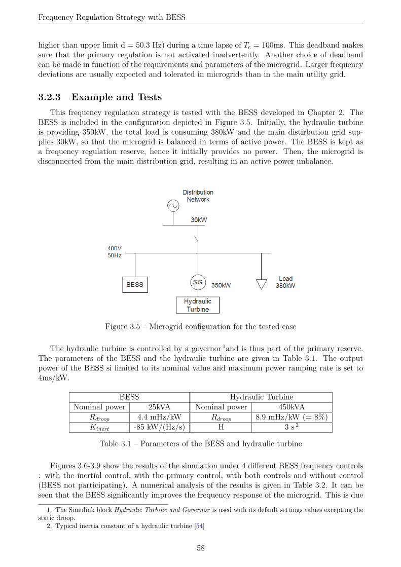
Frequency Regulation Strategy with BESS
higher than upper limit d = 50.3 Hz) during a time lapse of Tc = 100ms. This deadband makessure that the primary regulation is not activated inadvertently. Another choice of deadbandcan be made in function of the requirements and parameters of the microgrid. Larger frequencydeviations are usually expected and tolerated in microgrids than in the main utility grid.
3.2.3 Example and TestsThis frequency regulation strategy is tested with the BESS developed in Chapter 2. The
BESS is included in the configuration depicted in Figure 3.5. Initially, the hydraulic turbineis providing 350kW, the total load is consuming 380kW and the main distirbution grid sup-plies 30kW, so that the microgrid is balanced in terms of active power. The BESS is kept asa frequency regulation reserve, hence it initially provides no power. Then, the microgrid isdisconnected from the main distribution grid, resulting in an active power unbalance.
Figure 3.5 – Microgrid configuration for the tested case
The hydraulic turbine is controlled by a governor 1and is thus part of the primary reserve.The parameters of the BESS and the hydraulic turbine are given in Table 3.1. The outputpower of the BESS si limited to its nominal value and maximum power ramping rate is set to4ms/kW.
BESS Hydraulic TurbineNominal power 25kVA Nominal power 450kVA
Rdroop 4.4 mHz/kW Rdroop 8.9 mHz/kW (= 8%)Kinert -85 kW/(Hz/s) H 3 s 2
Table 3.1 – Parameters of the BESS and hydraulic turbine
Figures 3.6-3.9 show the results of the simulation under 4 different BESS frequency controls: with the inertial control, with the primary control, with both controls and without control(BESS not participating). A numerical analysis of the results is given in Table 3.2. It can beseen that the BESS significantly improves the frequency response of the microgrid. This is due
1. The Simulink block Hydraulic Turbine and Governor is used with its default settings values excepting thestatic droop.
2. Typical inertia constant of a hydraulic turbine [54]
58

Frequency Regulation Strategy with BESS
to the fact that the BESS brings additional frequency regulation reserve and has a much fasterresponse time than the hydraulic turbine. The inertial control raises the nadir and decreasesthe ROCOF right after the disturbance. The primary control improves the overall responseand has the additional effect to reduce the duration to reach steady state and increases thesteady-state frequency.
time[s]
0 5 10 15 20 25 30 35 40 45 50
Fre
quen
cy[H
z]
46
46.5
47
47.5
48
48.5
49
49.5
50
50.5
Both controls
Primary control
Inertia control
No control
Figure 3.6 – Microgrid frequency responseunder different frequency controls
time[s]
0 5 10 15 20 25 30 35 40 45 50R
OC
OF
[Hz/s
]
-0.8
-0.6
-0.4
-0.2
0
0.2
0.4
0.6
Both controls
Primary control
Inertial control
No control
Figure 3.7 – Microgrid ROCOF under dif-ferent frequency controls
time[s]
0 5 10 15 20 25 30 35 40 45 50
BE
SS
Pow
er[
kW
]
0
5
10
15
20
25
Both controls
Primary control
Inertial control
No control
Figure 3.8 – BESS power under differentfrequency controls
time[s]
0 5 10 15 20 25 30 35 40 45 50
Hydra
ulic
Turb
ine
Add
itio
na
l P
ow
er[
kW
]
-10
0
10
20
30
40
50
60
Both controls
Primary control
Inertial control
No control
Figure 3.9 – Hydraulic turbine additionalpower under different frequency controls
Nadir Average ROCOF(before nadir)
Steady-stateFrequency
Duration to ReachSteady-state 3
Both controls 49.22 Hz -0.15 Hz/s 49.91 Hz 14.5 sPrimary control 49.12 Hz -0.19 Hz/s 49.91 Hz 13.4 sInertial control 47.94 Hz -0.15 Hz/s 49.73 Hz 44.5 sNo control 46.29 Hz -0.50 Hz/s 49.73 Hz 43.0 s
Table 3.2 – Comparison of numerical results with different controls
3. The steady state is considered to be reached when the frequency stabilizes in a ± 0.05 Hz interval aroundthe steady-state frequency.
59

Chapter 4
Conclusion
A complete electrical model of a BESS was developed in this thesis. It includes the followingelements :
• Li-ion Battery & BMS : An equivalent electrical circuit composed of resistors andcapacitors was used to model the battery. The value of the parameters obtained inArticle [28] for one Li-ion celle were utilized. Then, an example of realistic Li-ion batterymodel (25kW, 34kWh) was built by mounting a certain number of Li-ion cells in seriesand parallel. The main purpose of the model is to reproduce the dynamic behaviour ofthe battery but it also provides a SOC estimation. The BMS is indissociable from itsbattery and its role is to protect, monitor and stabilize the battery. For instance, theBMS limits the current when the SOC is above/below a certain threshold to proventovercharge/over-discharge.
• DC/DC Converter : The topology chosen is the DAB converter with full bridges onboth sides. This converter is bidirectional and is a good compromise between efficiency,cost and power denstiy [35]. The lossless model of the converter is used and the simplestmodulation technique (phase shift modluation) is considered. LC filters are used onboth sides of the converter to smoothen the battery and DC link current. From there,an average dynamic model of the converter is built and compared with the full model.
• Battery-side Controller : A PI controller regulates the output power of the batteryby controlling the phase shift of the DAB converter.
• DC link : The DC link is simply composed of a relatively large capacitance. It allowsto filter the current harmonics which are not totally eliminated by the LC filters. It alsoprovides some sort of decoupling between the battery and grid sides of the sytem. Inlarger systems, other DERs or ESS can be connected to the same DC link.
• DC/AC Converter : The topology chosen is the three-phase voltage source inverterwith PWM modulation. It allows for bidirectional power flow. LC filters are placed onboth sides of the converter. The AC side filter is particularly important as it directlyimpacts the harmonic content of the grid current.
• Grid-side Controller : This controller is composed of an outer slower control loop andan inner faster control loop. The DC link and Q controllers form the outer loop. Theyare both PI controllers and respectively regulate the DC link voltage (thus active powerbalance) and reactive power. They generate the reference currents in the dq frame. Theinner loop contols the the grid current. The control is performed in the stationary (αβ)frame with PR controllers and the 5th and 7th harmonic currents are regulated as well.This inner loop generates the modulating signal for the inverter. The parameters of thePR controllers have to be chosen carefully to make sure there is no instability due toresonance with the output LC filter. Synchronization is performed with an EPLL whichis more robust against harmonics and unbalance than classic PLLs.
60

Tests on the overall system showed that, with the chosen parameters values, the BESS is robustagainst perturbations such as unbalance and harmonics. Moreover, the harmonic content ofthe grid current is relatively low.
The model was tested on a real-time simulation platform (Power hardware in the loop,owned by Laborelec). The average dynamic models were used for both converters to reducecomputational cost. The fact that the model could be successfully simulated in real-time (nooverruns) proves the feasibility of the designed controllers.
Finally, a small simple microgrid was built, composed of the BESS, a group of loads and ahydraulic turbine. For the test, the microgrid is considered to be disconnected from the mainutility grid, which implies an active power unbalance. The tests show that developed BESSmodel can be effectively be integrated in a larger power system and work properly. Moreover,the results proves the interest of using a BESS for frequency regulation in a microgrid. Sincethe BESS provides additional frequency regulation reserve and has a much faster response timethan the hydraulic turbine, it significantly improves the frequency response of the microgrid.
As mentioned in Section 1.3, this model will be utilized by Laborelec for some of theirprojects. They will have the opportunity to further improve and validate this model by runningexperimental tests on Li-ion batteries and simulate the model in more complex power systems.The approach of the model is rather systemic and does not go into the precise design of thepower electronics components. This emphasis of the model was intentionally placed on dynamicperformances and power quality considerations, but other aspects such as efficiency and costscould be examined in more details for the model.
61

Appendix A
Three-phase Inverter DC Current
Starting from the three balanced phase voltages given in Equations (2.44-2.46), the two linevoltages are then :
〈vm1(t)〉 = m1(t)VDC/2 = Umsin(ωt− π/6 + ϕ) (A.1)
〈vm2(t)〉 = m2(t)VDC/2 = Umsin(ωt− π/2 + ϕ) (A.2)
If the currents are balanced as well, we have :
〈i′a(t)〉 = I ′sin(ωt+ ψ) (A.3)
〈i′b(t)〉 = I ′sin(ωt− 2π/3 + ψ) (A.4)
Finally, the power conservation equation (2.40) becomes
VDC〈i(t)〉 = UmI′sin(ωt− π/6 + ϕ)sin(ωt+ ψ) + UmI
′sin(ωt− π/2 + ϕ)sin(ωt− 2π/3 + ψ)
= UmI′
2 (cos(ϕ− ψ − π/6)− cos(2ωt+ ϕ+ ψ − π/6)) +
UmI′
2 (cos(ϕ− ψ + π/6)− cos(2ωt+ ϕ+ ψ − 7π/6))
= UmI′
2 (cos(ϕ− ψ − π/6) + cos(ϕ− ψ + π/6))(A.5)
This proves that, in case of balanced system, the DC current has no 2ω component, unlike withsingle-phase inverter. However, if the system is unbalanced, there is a 2ω component.
62

Appendix B
Influence of DC/DC Converter andBattery-side Controller Parameters
The influence of the DC/DC converter and battery-side controller parameters is examinedin this appendix. The output battery power PLV and DC link power PHV are anaalyzed fordifferent set of parameters. The parameters are referred to the diagram shown in Figure 2.18.The system is tested in closed-loop. Excepting the parameter of interest, the values of the otherparameters are the same as in Subsection 2.3.6.
DAB Converter ParametersFigures B.1 and B.2 show that increasing the filter capacitances decreases the overshoots
of PLV and PHV . Figures B.3 and B.4 show that increasing the filter inductances increasesthe initial oscillations and overshoots. In fact, as shown in Equation 2.19, the damping ratioincreases when C increases and L decreases. For optimal design, the capacitance should thusbe as large as possible, taking into account constraints of size and cost. The inductance shouldnot to be too large, but large enough to effectively filter HF components.
time[s]
0 0.1 0.2 0.3
PLV[k
W]
0
5
10
15
20
25
C1 = 0.5 mF
time[s]
0 0.1 0.2 0.30
5
10
15
20
25
C1 = 1 mF
time[s]
0 0.1 0.2 0.30
5
10
15
20
25
C1 = 4 mF
Figure B.1 – PLV after a Pref step of 25kW for different values of C1
63
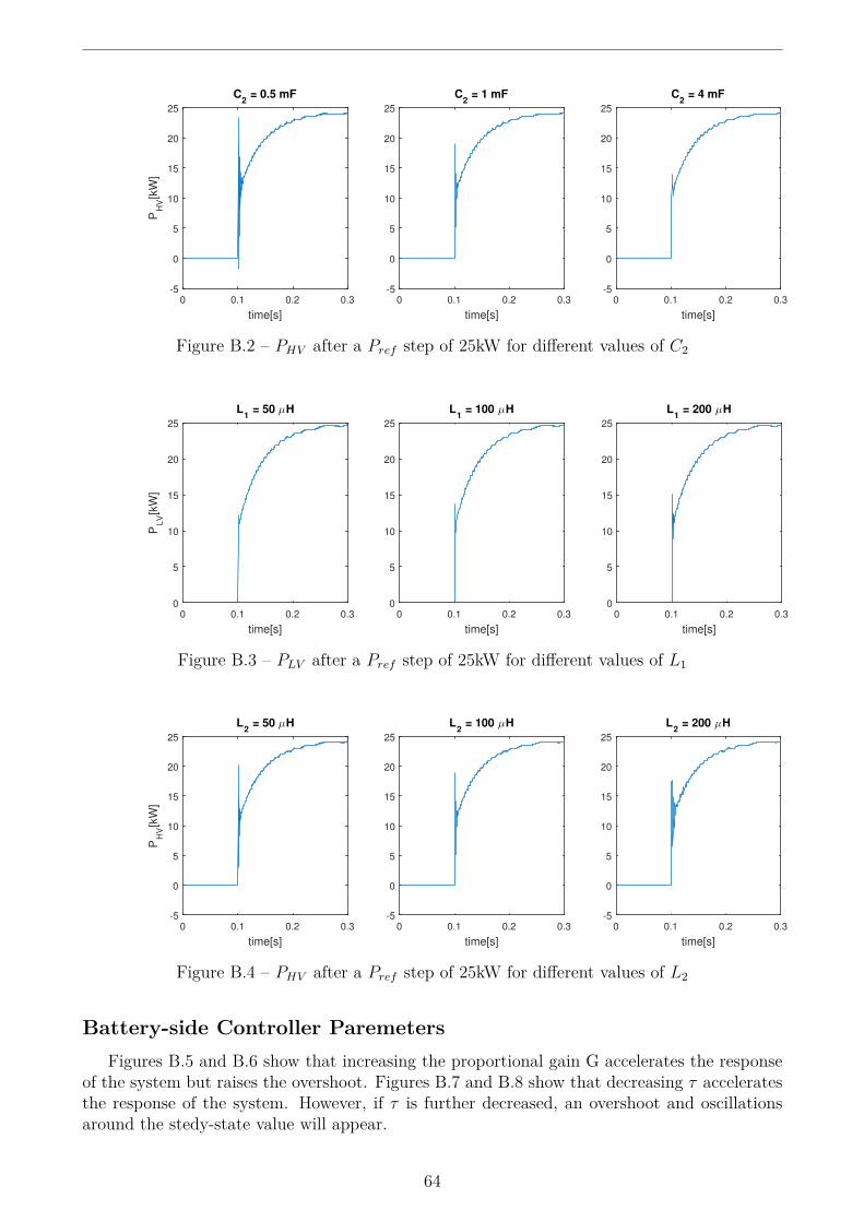
time[s]
0 0.1 0.2 0.3
PH
V[k
W]
-5
0
5
10
15
20
25
C2 = 0.5 mF
time[s]
0 0.1 0.2 0.3-5
0
5
10
15
20
25
C2 = 1 mF
time[s]
0 0.1 0.2 0.3-5
0
5
10
15
20
25
C2 = 4 mF
Figure B.2 – PHV after a Pref step of 25kW for different values of C2
time[s]
0 0.1 0.2 0.3
PLV[k
W]
0
5
10
15
20
25
L1 = 50 µH
time[s]
0 0.1 0.2 0.30
5
10
15
20
25
L1 = 100 µH
time[s]
0 0.1 0.2 0.30
5
10
15
20
25
L1 = 200 µH
Figure B.3 – PLV after a Pref step of 25kW for different values of L1
time[s]
0 0.1 0.2 0.3
PH
V[k
W]
-5
0
5
10
15
20
25
L2 = 50 µH
time[s]
0 0.1 0.2 0.3-5
0
5
10
15
20
25
L2 = 100 µH
time[s]
0 0.1 0.2 0.3-5
0
5
10
15
20
25
L2 = 200 µH
Figure B.4 – PHV after a Pref step of 25kW for different values of L2
Battery-side Controller ParemetersFigures B.5 and B.6 show that increasing the proportional gain G accelerates the response
of the system but raises the overshoot. Figures B.7 and B.8 show that decreasing τ acceleratesthe response of the system. However, if τ is further decreased, an overshoot and oscillationsaround the stedy-state value will appear.
64

time[s]
0 0.1 0.2 0.3
PLV[k
W]
0
5
10
15
20
25G = 0.45 deg/kW
time[s]
0 0.1 0.2 0.30
5
10
15
20
25G = 0.9 deg/kW
time[s]
0 0.1 0.2 0.3-5
0
5
10
15
20
25
30G = 1.8 deg/kW
Figure B.5 – PLV after a Pref step of 25kW for different values of G
time[s]
0 0.1 0.2 0.3
PH
V[k
W]
-5
0
5
10
15
20
25G = 0.45 deg/kW
time[s]
0 0.1 0.2 0.3-5
0
5
10
15
20
25G = 0.9 deg/kW
time[s]
0 0.1 0.2 0.3-5
0
5
10
15
20
25G = 1.8 deg/kW
Figure B.6 – PHV after a Pref step of 25kW for different values of G
time[s]
0 0.1 0.2 0.3
PLV[k
W]
-5
0
5
10
15
20
25
30τ = 10 ms
time[s]
0 0.1 0.2 0.30
5
10
15
20
25τ = 20 ms
time[s]
0 0.1 0.2 0.30
5
10
15
20
25τ = 40 ms
Figure B.7 – PLV after a Pref step of 25kW for different values of τ
65

time[s]
0 0.1 0.2 0.3
PH
V[k
W]
-5
0
5
10
15
20
25τ = 10 ms
time[s]
0 0.1 0.2 0.3-5
0
5
10
15
20
25τ = 20 ms
time[s]
0 0.1 0.2 0.3-5
0
5
10
15
20
25τ = 40 ms
Figure B.8 – PHV after a Pref step of 25kW for different values of τ
66

Appendix C
Influence of Grid Impendance, OutputLC filter and Grid-side ControllerParemeters
The influence of the grid impedance, output LC filter and grid-side controller parametersis examined in this appendix. The effect of these paremeters on the stability of the currentcontrol is considered. The parameters are referred to the diagram shown in Figure 2.43 andthe controller transfer function given in Equation 2.60. The system is tested in closed-loop.Excepting the parameter of interest, the values of the other parameters are the same as inSubsections 2.4.3 and 2.5.5.
Grid ImpedanceThe variation of the natural frequency fn2 (Eq 2.53) of the output LC filter with the grid
inductance L is depicted in Figure C.1. Figures C.2 and C.3 show how that there are overallmore harmonics when L is smaller. The influence of the grid resistance R on the harmoniccontent is negligible.
Figure C.4 shows the position of the poles of the closed-loop system as a function of L.Increasing L gets all the poles closer to the imaginary axis. When a certain value of L isreached, two poles have positive real part, hence the system becomes unstable. On the otherhand, as shown in Figure C.5, R has a stabilizing effect and, as it increases, gets the polesfurther away from the imaginary axis. If the resistance is too small, the system might beunstable.
67

Grid Inductance[mH]
0 0.5 1 1.5 2 2.5
Natu
ral F
requ
ency[H
z]
1200
1300
1400
1500
1600
1700
1800
1900
2000
Figure C.1 – Variation of fn2 with L
Figure C.2 – Fourier analysis of ires1 with L = 0.25mH
Figure C.3 – Fourier analysis of ires1 with L = 1mH
68
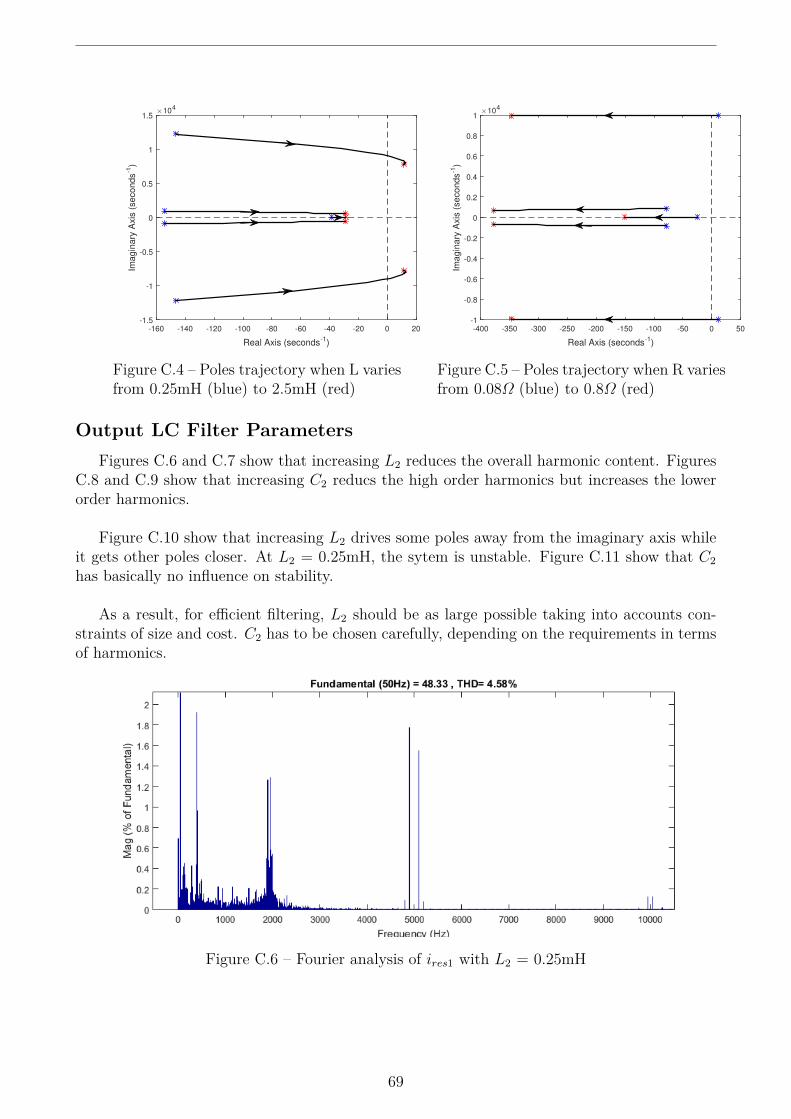
Real Axis (seconds-1)
-160 -140 -120 -100 -80 -60 -40 -20 0 20
Imagin
ary
Axis
(second
s-1
)
×104
-1.5
-1
-0.5
0
0.5
1
1.5
Figure C.4 – Poles trajectory when L variesfrom 0.25mH (blue) to 2.5mH (red)
Real Axis (seconds-1)
-400 -350 -300 -250 -200 -150 -100 -50 0 50
Imagin
ary
Axis
(second
s-1
)
×104
-1
-0.8
-0.6
-0.4
-0.2
0
0.2
0.4
0.6
0.8
1
Figure C.5 – Poles trajectory when R variesfrom 0.08Ω (blue) to 0.8Ω (red)
Output LC Filter ParametersFigures C.6 and C.7 show that increasing L2 reduces the overall harmonic content. Figures
C.8 and C.9 show that increasing C2 reducs the high order harmonics but increases the lowerorder harmonics.
Figure C.10 show that increasing L2 drives some poles away from the imaginary axis whileit gets other poles closer. At L2 = 0.25mH, the sytem is unstable. Figure C.11 show that C2has basically no influence on stability.
As a result, for efficient filtering, L2 should be as large possible taking into accounts con-straints of size and cost. C2 has to be chosen carefully, depending on the requirements in termsof harmonics.
Figure C.6 – Fourier analysis of ires1 with L2 = 0.25mH
69

Figure C.7 – Fourier analysis of ires1 with L2 = 1mH
Figure C.8 – Fourier analysis of ires1 with C2 = 20µF
Figure C.9 – Fourier analysis of ires1 with C2 = 80µF
70

Real Axis (seconds-1)
-160 -140 -120 -100 -80 -60 -40 -20 0 20
Imagin
ary
Axis
(second
s-1
)
×104
-1.5
-1
-0.5
0
0.5
1
1.5
Figure C.10 – Poles trajectory when L2varies from 0.25mH (blue) to 2.5mH (red)
Real Axis (seconds-1)
-120 -110 -100 -90 -80 -70 -60 -50 -40 -30 -20
Imagin
ary
Axis
(second
s-1
)
×104
-2
-1.5
-1
-0.5
0
0.5
1
1.5
2
Figure C.11 – Poles trajectory when C2varies from 10µF (blue) to 100µF (red)
Grid-side Controller ParametersFigure C.12 shows that dynamics is influenced by the parameter KI . Increasing KI acceler-
ates the response but can lead to an overshoot if it is too high. Parameters KP and ωc do notinfluence this kind of test as the gain at the fundamental frequency is mainly determined by KI .
Figures C.13, C.14 and C.15 show that all the paremeters influence the stability by drivingsome poles away while taking other poles closer. The choice of parameters to ensure andoptimize stability performances is thus complex.
time[s]
0 0.1 0.2 0.3 0.4
i res1[A
]
-60
-40
-20
0
20
40
60
KI = 1000
time[s]
0 0.1 0.2 0.3 0.4-60
-40
-20
0
20
40
60
KI = 3000
time[s]
0 0.1 0.2 0.3 0.4-80
-60
-40
-20
0
20
40
60
80
KI = 10000
Figure C.12 – Grid current ires1 with a pulse of id,ref from t=0.1s to t=0.3s with differentvalues of KI
71

Real Axis (seconds-1)
-160 -140 -120 -100 -80 -60 -40 -20 0 20 40
Imagin
ary
Axis
(second
s-1
)
×104
-1
-0.8
-0.6
-0.4
-0.2
0
0.2
0.4
0.6
0.8
1
Figure C.13 – Poles trajectory when KI
varies from 1000 (blue) to 10000 (red)
Real Axis (seconds-1)
-160 -140 -120 -100 -80 -60 -40 -20 0 20 40
Imagin
ary
Axis
(second
s-1
)
×104
-1
-0.8
-0.6
-0.4
-0.2
0
0.2
0.4
0.6
0.8
1
Figure C.14 – Poles trajectory when KP
varies from 0 (blue) 0.2 (red)
Real Axis (seconds-1)
-160 -140 -120 -100 -80 -60 -40 -20 0 20 40
Imagin
ary
Axis
(seconds
-1)
×104
-1
-0.8
-0.6
-0.4
-0.2
0
0.2
0.4
0.6
0.8
1
Figure C.15 – Poles trajectory when ωc varies from 0.05 (blue) 0.5 (red)
72
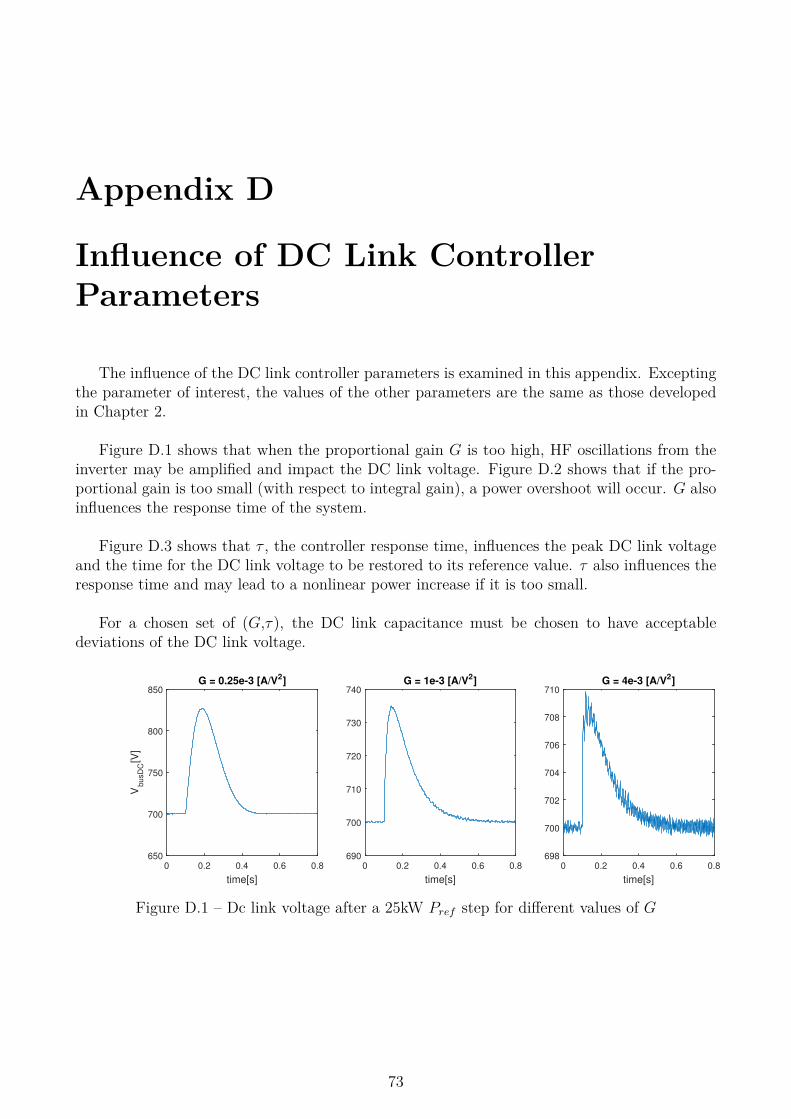
Appendix D
Influence of DC Link ControllerParameters
The influence of the DC link controller parameters is examined in this appendix. Exceptingthe parameter of interest, the values of the other parameters are the same as those developedin Chapter 2.
Figure D.1 shows that when the proportional gain G is too high, HF oscillations from theinverter may be amplified and impact the DC link voltage. Figure D.2 shows that if the pro-portional gain is too small (with respect to integral gain), a power overshoot will occur. G alsoinfluences the response time of the system.
Figure D.3 shows that τ , the controller response time, influences the peak DC link voltageand the time for the DC link voltage to be restored to its reference value. τ also influences theresponse time and may lead to a nonlinear power increase if it is too small.
For a chosen set of (G,τ), the DC link capacitance must be chosen to have acceptabledeviations of the DC link voltage.
time[s]
0 0.2 0.4 0.6 0.8
VbusD
C[V
]
650
700
750
800
850G = 0.25e-3 [A/V2]
time[s]
0 0.2 0.4 0.6 0.8690
700
710
720
730
740G = 1e-3 [A/V2]
time[s]
0 0.2 0.4 0.6 0.8698
700
702
704
706
708
710G = 4e-3 [A/V2]
Figure D.1 – Dc link voltage after a 25kW Pref step for different values of G
73

time[s]
0 0.2 0.4 0.6 0.8
Pre
s[k
W]
-5
0
5
10
15
20
25
30G = 0.25e-3 [A/V2]
time[s]
0 0.2 0.4 0.6 0.8-5
0
5
10
15
20
25G = 1e-3 [A/V2]
time[s]
0 0.2 0.4 0.6 0.8-5
0
5
10
15
20
25G = 4e-3 [A/V2]
Figure D.2 – Output power Pres after a 25kW Pref step for different values of G
time[s]
0 0.2 0.4 0.6 0.8
VbusD
C[V
]
695
700
705
710
715
720τ = 10ms
time[s]
0 0.2 0.4 0.6 0.8695
700
705
710
715
720
725
730τ = 50ms
time[s]
0 0.2 0.4 0.6 0.8690
700
710
720
730
740
750τ = 250ms
Figure D.3 – Dc link voltage after a 25kW Pref step for different values of τ
time[s]
0 0.2 0.4 0.6 0.8
Pre
s[k
W]
-5
0
5
10
15
20
25τ = 10ms
time[s]
0 0.2 0.4 0.6 0.8-5
0
5
10
15
20
25τ = 50ms
time[s]
0 0.2 0.4 0.6 0.8-5
0
5
10
15
20
25τ = 250ms
Figure D.4 – Output power Pres after a 25kW Pref step for different values of τ
74
Bibliography
[1] "History Of Batteries : A Timeline" (2014, June). Retrieved from http://www.upsbatterycenter.com/blog/history-batteries-timeline/.
[2] Bruno Scrosati and Jürgen Garche, "Lithium batteries : status, prospects and future",Journal of Power Sources, vol. 195, pp. 2419–2430, 2010.
[3] Epec, "Battery cell comparison". Retrieved from http://www.epectec.com/batteries/cell-comparison.html, consulted the 4th of May 2017
[4] James F. Rohan, Maksudul Hasan, Sanjay Patil, Declan P. Casey and Tomás Clancy,"Energy Storage: Battery Materials and Architectures at the Nanoscale", ICT - Energy -Concepts Towards Zero - Power Information and Communication Technology, 2014.
[5] U.S. Department of Energy, "The History of the Electric Car". Retrieved from https://www.energy.gov/public-services/vehicles, consulted the 5th of May 2017.
[6] David W. Gao, Energy Storage for Sustainable Microgrid. Academic Press, 2015.[7] Gold Peak Industries Ltd., "Lithium Ion Technical Book", 2000.[8] Cutler Cleveland and Christopher J. Morris, Dictionary of Energy. Amsterdam: Elsevier,
p. 473, 2006.[9] "Car Prototype Generates Electricity, And Cash" (2007, December), Science Daily. Re-
trieved from https://www.sciencedaily.com/releases/2007/12/071203133532.htm.[10] Dan T.Ton and Merill A.Smith, "The U.S. Department of Energy Microgrid Initiative",
The Electricity Journal, vol. 25, pp. 84-94, 2012.[11] Xiong Liu, Peng Wang and Poh Chiang Loh, "A Hybrid AC/DC Microgrid", Nanyang
Technological University, Singapore, 2010.[12] Claudio A. Cañizares, "Trends in Microgrid Control", IEEE Transactions on Smart Grid,
vol. 5, no. 4, pp. 1905-1919, 2014.[13] U.S. Department of Energy, "DOE Global Energy Storage Database". Retrieved from www.
energystorageexchange.org.[14] R.S Khurmi, Materials Science. S.Chand & Company, 2014.[15] Ioannis Hadjipaschalis, Andreas Poullikkas and Venizelos Efthimiou, "Overview of current
and future energy storage technologies for electric power applications", Renewable andSustainable Energy Reviews, vol. 13, 2008.
[16] Edward Barbour, "Energy Storage Technologies Explained". Retrieved from http://energystoragesense.com/energy-storage-technologies/, consulted the 9th of May2017.
[17] J. Bélanger, P. Venne and J.-N. Paquin, "The What, Where and Why of Real-Time Sim-ulation", 2013.
[18] Chris Caerts, "Web-of-Cells Concept and Control Scheme (part 1)" (2016). Retrieved fromhttp://www.electrairp.eu/index.php?option=com_content&view=article&id=354.
75

BIBLIOGRAPHY
[19] Matthew T. Lawder, Bharatkumar Suthar, Paul W. C. Northrop, Sumitava De, C. MichaelHoff, Olivia Leitermann, Mariesa L. Crow, Shriram Santhanagopalan and Venkat R. Sub-ramanian, "Battery Energy Storage System (BESS) and Battery Management System(BMS)for Grid-Scale Applications", Proceedings of the IEEE, vol. 102, no. 6, 2014.
[20] Math H.J. Bollen, Understanding Power Quality Problems. IEEE Press Series on PowerEngineering, 2000.
[21] Marshall Brain, "How Lithium-ion Batteries Work". Retrieved from http://electronics.howstuffworks.com/everyday-tech/lithium-ion-battery1.htm, consulted the 10th ofMay 2017.
[22] Chris Woodford, "Lithium-ion batteries" (2014, December). Retrieved from http://www.explainthatstuff.com/how-lithium-ion-batteries-work.html, consulted the 10th ofMay 2017.
[23] H.J. Bergveld, W.S. Kruijt and P.H.L. Notten, Battery Management Systems: Design byModelling. Eindhoven : Philips Research Laboratories, 2002.
[24] David Linden and Thomas Reddy, Handbook of batteries. McGraw-Hill, 2001.[25] Daniel H. Doughty and Chris C. Crafts, "FreedomCAR Electrical Energy Storage System
Abuse Test Manual for Electric and Hybrid Electric Vehicle Applications", Sandia NationalLaboratories, 2006.
[26] Yuan Zou, Xiaosong Hu, Hongmin Ma and Shengbo Eben Li, "Combined State of Chargeand State of Health estimation over lithium-ion battery cell cycle lifespan for electricvehicles", Journal of Power Sources, vol. 273, pp. 793-803, 2015.
[27] D. W. Dennis, V. S. Battaglia and A. Belanger, “Electrochemical modeling of lithiumpolymer batteries”, Journal of Power Sources, vol. 110, pp. 310–320, 2002.
[28] Ryan C. Kroeze and Philip T. Krein, "Electrical Battery Model for Use in Dynamic ElectricVehicle Simulations", University of Illinois, 2008.
[29] P. Rong and M. Pedram, “An analytical model for predicting the remaining battery ca-pacity of lithium-ion batteries", University of Southern California, 2003.
[30] Hongwen He, Rui Xiong and Jinxin Fan, "Evaluation of Lithium-Ion Battery EquivalentCircuit Models for State of Charge Estimation by an Experimental Approach", Energies,vol. 4, pp. 582-598, 2011.
[31] Mohsen Mousavi, Shaikh Hoque, Shahryar Rahnamayan, Ibrahim Dincer, Greg F. Naterer,"Optimal Design of an Air-Cooling System for a Li-Ion Battery Pack in Electric Vehicleswith a Genetic Algorithm", in Proceedings of the IEEE Congress on Evolutionary Com-putation, 2000.
[32] E. Sarasketa-Zabala, E. Martinez-Laserna, M. Berecibar, I. Gandiaga, L.M. Rodriguez-Martinez, I. Villarreal,"Realistic lifetime prediction approach for Li-ion batteries", AppliedEnergy, vol. 162, pp. 839-852, 2015.
[33] Battery University, "BU-802b: What does Elevated Self-discharge Do?" (2017,April). Retrieved from http://batteryuniversity.com/learn/article/elevating_self_discharge.
[34] Panasonic, CGR18650AF datasheet. Retrieved from http://www.datasheetarchive.com/pdf/download.php?id=66592976dbf72936a88cde4c94c9b19d803011&type=P&query=CGR18650A.
[35] Florian Krismer, "Modeling and Optimization of Bidirectional Dual Active Bridge DC–DCConverter Topologies", PhD thesis, ETH Zurich, 2010.
76
BIBLIOGRAPHY
[36] G. Chen, Y.-S. Lee, S. Y. R. Hui, D. Xu and Y. Wang, “Actively clamped bidirectionalflyback converter”, IEEE Transactions on Industrial Electronics, vol. 47, no. 4, 2000.
[37] Carl Blake and Chris Bull, "IGBT or MOSFET: Choose Wisely", Infineon, 2003.[38] Infineon, "IGBT Selection Guide", Retrieved from http://www.infineon.com/
dgdl/Infineon-IGBT_Discretes_Selection_Guide-SG-v00_00-EN.pdf?fileId=db3a3043324cae8c01326cea43bc17bc.
[39] Federico Ibáñez, Javier Vadillo, Miguel Martínez-Iturralde Maiza and José Martín Echev-erría, "30kW DC-DC Converters with Regenerative Mode for Electric Cars", Journal ofPower Electronics, vol. 12, pp. 233-241, 2012.
[40] Texas Instruments, "Phase-Shifted Full Bridge DC/DC Power Converter Design Guide",2014.
[41] Sayed Ali Khajehoddin, Masoud Karimi Ghartemani, Praveen Jain and Alireza Bakhsai,"Distributed Power Generation Interface", U.S. Patent 8,668,287 B2.
[42] John Cheng, "IEEE Standard 519-2014", Schneider. Retrieved from http://www.schneider-electric.com.tw/documents/Event/2016_electrical_engineering_seminar/IEEE_STD_519_1992vs2014.pdf, consulted the 7th of June 2017.
[43] N. A. Rahim and S. Mekhilef, "High Efficiency THIPWM Three-Phase Inverter for GridConnected System", In Proc. IEEE Symposium on Industrial Electronics and Applications,2010.
[44] Witold Mazgaj, Bartosz Rozegnal and Zbigniew Szular, "Switching Losses in Three-phaseVoltage Source Inverters", 2015.
[45] Frede Blaabjerg, Remus Teodorescu, Marco Liserre and Adrian V. Timbus, "Overviewof Control and Grid Synchronization for Distributed Power Generation Systems", IEEETransactions on Industrial Electronics, vol. 53, no. 5, 2006.
[46] Remus Teodorescu, Frede Blaabjerg and Marco Liserre, "Proportional-Resonant Con-trollers : A New Breed of Controllers Suitablefor Grid-Connected Voltage-Source Con-verters", Proceedings of The 9th International Conference on Optimization of Electricaland Electronic Equipments, 2004.
[47] Masoud Karimi-Ghartemani, Enhanced Phase-locked Loop Structures for Power and En-ergy Applications. Wiley IEEE Press Series on Microelectronic Systems, 2014.
[48] Mojgan Nikouie, Oskar Wallmark, Lebing Jin and Hans-Peter Nee, "A DC-link VoltageControl Scheme for Single-phase Grid-connected PV Inverters", Proceedings of EnergyConversion Congress and Exposition, 2011.
[49] Kyung Soo K, McKenzie KJ, Yilu L and Atcitty S., "A study on applications of energystorage for the wind power operation in power systems", Proc. IEEE Power EngineeringSociety General Meeting, 2006.
[50] Wei L and Joos G., "Performance comparison of aggregated and distributed energy storagesystems in a wind farm for wind power fluctuation suppression", Proc. Power EngineeringSociety General Meeting, 2007.
[51] Aneel Kumar Akhani, "Primary Secondary and Tertiary Frequency Con-trol". Retrieved from http://top10electrical.blogspot.be/2015/10/primary-secondary-and-tertiary.html, consulted the 29th of May 2017.
[52] Hugues Chanoine, "Frequency regulation: the need for fast respond-ing assets and the “mileage” case in the USA" (2013, Septem-ber). Retrieved from http://www.cleanhorizon.com/blog/2013/09/frequency-regulation-the-need-for-fast-responding-assets-and-the-mileage-case\-in-the-usa/.
77

BIBLIOGRAPHY
[53] Prabha Kundur, Power System Stability and Control. Electric Power Research Institute,1994.
[54] D.P.Kothari and I.J. Nagrath, Modern Power System Analysis. McGraw-Hill, 1980.
78