1

R for beginners

Emmanuel Paradis

1 What is R ? 3

2 The few things to know before starting 52.1 The operator <- 52.2 Listing and deleting the objects in memory 52.3 The on-line help 6

3 Data with R 83.1 The ‘objects’ 83.2 Reading data from files 83.3 Saving data 103.4 Generating data 11

3.4.1 Regular sequences 113.4.2 Random sequences 13

3.5 Manipulating objects 133.5.1 Accessing a particular value of an object 133.5.2 Arithmetics and simple functions 143.5.3 Matrix computation 16

4 Graphics with R 184.1 Managing graphic windows 18

4.1.1 Opening several graphic windows 184.1.2 Partitioning a graphic window 18

4.2 Graphic functions 194.3 Low-level plotting commands 204.4 Graphic parameters 21

5 Statistical analyses with R 23

6 The programming language R 266.1 Loops and conditional executions 266.2 Writing you own functions 27

7 How to go farther with R ? 30

8 Index 31

2

The goal of the present document is to give a starting point for people newly interested in R. Itried to simplify as much as I could the explanations to make them understandables by all,while giving useful details, sometimes with tables. Commands, instructions and examples arewritten in Courier font.

I thank Julien Claude, Christophe Declercq, Friedrich Leisch and Mathieu Ros for theircomments and suggestions on an earlier version of this document. I am also grateful to all themembers of the R Development Core Team for their considerable efforts in developing R andanimating the discussion list ‘r-help’. Thanks also to the R users whose questions orcomments helped me to write “R for beginners”.

© 2000, Emmanuel Paradis (20 octobre 2000)

3

1 What is R ?

R is a statistical analysis system created by Ross Ihaka & Robert Gentleman (1996, J.Comput. Graph. Stat., 5: 299-314). R is both a language and a software; its most remarkablefeatures are:

• an effective data handling and storage facility,• a suite of operators for calculations on arrays, matrices, and other complex operations,• a large, coherent, integrated collection of tools for statistical analysis,• numerous graphical facilities which are particularly flexible, and• a simple and effective programming language which includes many facilities.

R is a language considered as a dialect of the language S created by the AT&T BellLaboratories. S is available as the software S-PLUS commercialized by MathSoft (seehttp://www.splus.mathsoft.com/ for more information). There are importants differences inthe conceptions of R and S, but they are not of interest to us here: those who want to knowmore on this point can read the paper by Gentleman & Ihaka (1996) or the R-FAQ(http://cran.r-project.org/doc/FAQ/R-FAQ.html), a copy of which is alse distributed with thesoftware.

R is freely distributed on the terms of the GNU Public Licence of the Free SoftwareFoundation (for more information: http://www.gnu.org/); its development and distribution arecarried on by several statisticians known as the R Development Core Team. A key-element inthis development is the Comprehensive R Archive Network (CRAN).

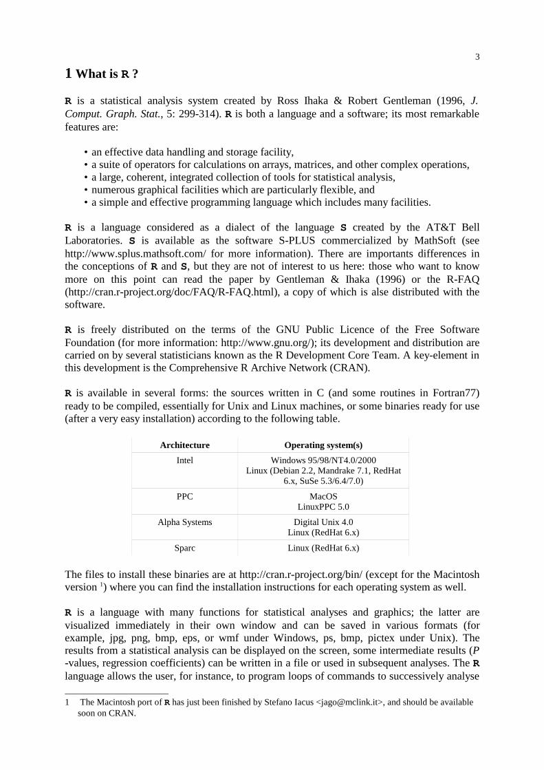
R is available in several forms: the sources written in C (and some routines in Fortran77)ready to be compiled, essentially for Unix and Linux machines, or some binaries ready for use(after a very easy installation) according to the following table.

Architecture Operating system(s)

Intel Windows 95/98/NT4.0/2000Linux (Debian 2.2, Mandrake 7.1, RedHat

6.x, SuSe 5.3/6.4/7.0)

PPC MacOSLinuxPPC 5.0

Alpha Systems Digital Unix 4.0Linux (RedHat 6.x)

Sparc Linux (RedHat 6.x)

The files to install these binaries are at http://cran.r-project.org/bin/ (except for the Macintoshversion 1) where you can find the installation instructions for each operating system as well.

R is a language with many functions for statistical analyses and graphics; the latter arevisualized immediately in their own window and can be saved in various formats (forexample, jpg, png, bmp, eps, or wmf under Windows, ps, bmp, pictex under Unix). Theresults from a statistical analysis can be displayed on the screen, some intermediate results (P-values, regression coefficients) can be written in a file or used in subsequent analyses. The Rlanguage allows the user, for instance, to program loops of commands to successively analyse

1 The Macintosh port of R has just been finished by Stefano Iacus <jago@mclink.it>, and should be availablesoon on CRAN.

4

several data sets. It is also possible to combine in a single program different statisticalfunctions to perform more complex analyses. The R users may benefit of a large number ofroutines written for S and available on internet (for example: http://stat.cmu.edu/S/), most ofthese routines can be used directly with R.

At first, R could seem too complex for a non-specialist (for instance, a biologist). This maynot be true actually. In fact, a prominent feature of R is its flexibility. Whereas a classicalsoftware (SAS, SPSS, Statistica, ...) displays (almost) all the results of an analysis, R storesthese results in an object, so that an analysis can be done with no result displayed. The usermay be surprised by thus, but such a feature is very useful. Indeed, the user can extract onlythe part of the results which is of interest. For example, if one runs a series of 20 regressionsand wants to compare the different regression coefficients, R can display only the estimatedcoefficients: thus the results will take 20 lines, whereas a classical software could well open20 results windows. One could cite many other examples illustrating the superiority of asystem such as R compared to classical softwares; I hope the reader will be convinced of thisafter reading this document.

5

2 The few things to know before starting

Once R is installed on your computer, the software is accessed by launching the correspondingexecutable (RGui.exe ou Rterm.exe under Windows, R under Unix). The prompt ‘>’ indicatesthat R is waiting for your commands.

Under Windows, some commands related to the system (accessing the on-line help, openingfiles, ...) can be executed via the pull-down menus, but most of them must heve to be typed onthe keyboard. We shall see in a first step three aspects of R: creating and modifying elements,listing and deleting objects in memory, and accessing the on-line help.

2.1 The operator <-

R is an object-oriented language: the variables, data, matrices, functions, results, etc. arestored in the active memory of the computer in the form of objects which have a name: onehas just to type the name of the object to display its content. For example, if an object n hasfor value 10 :

> n[1] 10

The digit 1 within brackets indicates that the display starts at the first element of n (see §3.4.1). The symbol assign is used to give a value to an object. This symbol is written with abracket (< or >) together with a sign minus so that they make a small arrow which can bedirected from left to right, or the reverse:

> n <- 15> n[1] 15> 5 -> n> n[1] 5

The value which is so given can be the result of an arithmetic expression:

> n <- 10+2> n[1] 12

Note that you can simply type an expression without assigning its value to an object, the resultis thus displayed on the screen but not stored in memory:

> (10+2)*5[1] 60

2.2 Listing and deleting the objects in memory

The function ls() lists simply the objects in memory: only the names of the objects aredisplayed.

> name <- "Laure"; n1 <- 10; n2 <- 100; m <- 0.5> ls()[1] "m" "n1" "n2" "name"

Note the use of the semi-colon ";" to separate distinct commands on the same line. If there are

6

a lot of objects in memory, it may be useful to list those which contain given character in theirname: this can be done with the option pattern (which can be abbreviated with pat) :

> ls(pat="m")[1] "m" "name"

If we want to restrict the list of objects whose names strat with this character:

> ls(pat="^m")[1] "m"

To display the details on the objects in memory, we can use the function ls.str():

> ls.str()m: num 0.5n1: num 10n2: num 100name: chr "name"

The option pattern can also be used as described above. Another useful option of ls.str()is max.level which specifies the level of details to be displayed for composite objects. Bydefault, ls.str() displays the details of all objects in memory, including the columns of dataframes, matrices and lists, which can result in a very long display. One can avoid to display allthese details with the option max.level=-1:

> M <- data.frame(n1,n2,m)> ls.str(pat="M")M: ‘data.frame’: 1 obs. of 3 variables: $ n1: num 10 $ n2: num 100 $ m: num 0.5> ls.str(pat="M", max.level=-1)M: ‘data.frame’: 1 obs. of 3 variables:

To delete objects in memory, we use the function rm(): rm(x) deletes the object x, rm(x,y)both objects x et y, rm(list=ls()) deletes objects in memory; the same options mentionedfor the function ls() can then be used to delete selectively some objects:rm(list=ls(pat="m")).

2.3 The on-line help

The on-line help of R gives some very useful informations on how to use the functions. Thehelp in html format is called by typing:

> help.start()

A search with key-words is possible with this html help. A search of functions can be donewith apropos("what") which lists the functions with "what" in their name:

> apropos("anova") [1] "anova" "anova.glm" "anova.glm.null" "anova.glmlist" [5] "anova.lm" "anova.lm.null" "anova.mlm" "anovalist.lm" [9] "print.anova" "print.anova.glm" "print.anova.lm" "stat.anova"

The help is available in text format for a given function, for instance:

7> ?lm

displays the help file for the function lm(). The function help(lm) or help("lm") has thesame effect. This last function must be used to access the help with non-conventionalcharacters:

> ?*Error: syntax error> help("*")Arithmetic package:base R Documentation

Arithmetic Operators...

8

3 Data with R

3.1 The ‘objects’

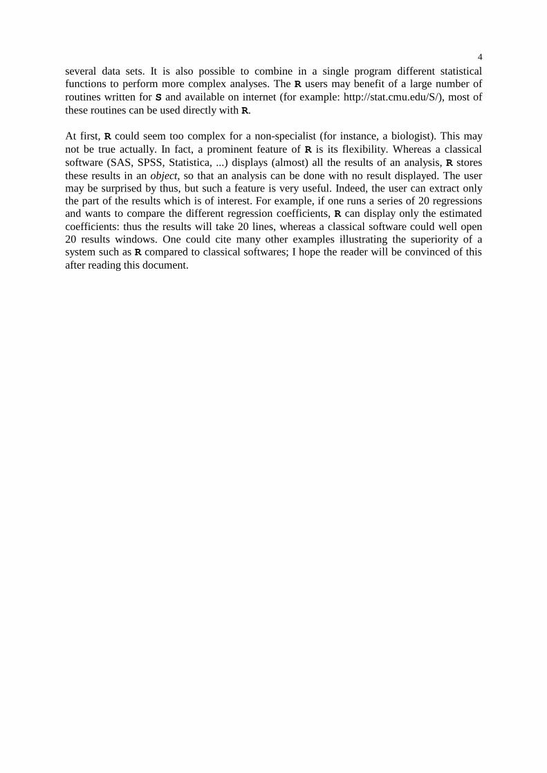
R works with objects which all have two intrinsic attributes: mode and length. The mode isthe kind of elements of an object; there are four modes: numeric, character, complex, andlogical. There are modes but these do not characterize data, for instance: function,expression, or formula. The length is the total number of elements of the object. Thefollowing table summarizes the differents objects manipulated by R.

object possible modes several modes possible inthe same object ?

vector numeric, character, complex, or logical No

factor numeric, or character No

array numeric, character, complex, or logical No

matrix numeric, character, complex, or logical No

data.frame numeric, character, complex, or logical Yes

ts numeric, character, complex, or logical Yes

list numeric, character, complex, logical, function, expression, orformula

Yes

A vector is a variable in the commonly admitted meaning. A factor is a categorical variable.An array is a table with k dimensions, a matrix being a particular case of array with k = 2.Note that the elements of an array or of a matrix are all of the same mode. A data.frame is atable composed with several vectors all of the same length but possibly of different modes. Ats time-series data set and so contains supplementary attributes such as the frequency and thedates.

Among the non-intrinsic attributes of an object, one is to be kept in mind: it is dim whichcorresponds to the dimensions of a multivariate object. For example, a matrix with 2 lines and2 columns has for dim the pair of values [2,2], but its length is 4.

It is useful to know that R discriminates, for the names of the objects, the upper-casecharacters from the lower-case ones (i.e., it is case-sensitive), so that x and X can be used toname distinct objects (even under Windows):

> x <- 1; X <- 10> ls()[1] "X" "x"> X[1] 10> x[1] 1

3.2 Lire des données à partir d’un fichier

R can read data stored in text (ASCII) files; three functions can be used: read.table()

(which has two variants: read.csv() and read.csv2()), scan() and read.fwf(). Forexample, if we have a file data.dat, one can just type:

> mydata <- read.table("data.dat")

9

mydata will then be a data.frame, and each variable will be named, by default, V1, V2, ...and could be accessed individually by mydata$V1, mydata$V2, ..., or by mydata["V1"],mydata["V2"], ..., or, still another solution, by mydata[,1], mydata[,2], etc2. There areseveral options available for the function read.table() which values by default (i.e. thoseused by R if omitted by the user) and other details are given in the following table:

> read.table(file, header=FALSE, sep="", quote="\"’", dec=".", row.names=,col.names=, as.is=FALSE, na.strings="NA", skip=0, check.names=TRUE,strip.white=FALSE)

file the name of the file (within ""), possibly with its path (the symbol \ is not allowed and mustbe replaced by /, even under Windows)

header a logical (FALSE or TRUE) indicating if the file contains the names of the variables on itsfirst line

sep the field separator used in the file, for instance sep="\t" if it is a tabulation

quote the characters used to cite the variables of mode character

dec the character used for the decimal point

row.names a vector with the names of the lines which can be a vector of mode character, or the number(or the name) of a variable of the file (by default: 1, 2, 3, ...)

col.names a vector with the names of the variables (by default: V1, V2, V3, ...)

as.is controls the conversion of character variables as factors (if FALSE) or keep them ascharacters (TRUE)

na.strings the value given to missing data (converted as NA)

skip the number of lines to be skipped before reading the data

check.names if TRUE, checks that the variable names are valid for R

strip.white (conditional to sep) if TRUE, scan deletes extra spaces before and after the charactervariables

Two variants of read.table() are useful because they have different by default options:

read.csv(file, header = TRUE, sep = ",", quote="\"", dec=".", ...)read.csv2(file, header = TRUE, sep = ";", quote="\"", dec=",", ...)

The function scan() is more flexible than read.table() and has more options. The maindifference is that it is possible to specify the mode of the variables, for example :

> mydata <- scan("data.dat", what=list("",0,0))

reads in the file data.dat three variables, the first is of mode character and the next two are ofmode numeric. The options are as follows.

> scan(file="", what=double(0), nmax=-1, n=-1, sep="", quote=if (sep=="\n")"" else "’\"", dec=".", skip=0, nlines=0, na.strings="NA", flush=FALSE,strip.white=FALSE, quiet=FALSE)

file the name of the file (within ""), possibly with its path (the symbol \ is not allowed and must bereplaced by /, even under Windows); if file="", the data are input with the keyboard (theentry is terminated with a blank line)

what specifies the mode(s) of the data

2 Nevertheless, there is a difference: mydata$V1 and mydata[,1] are vectors whereas mydata["V1"] is adata.frame.

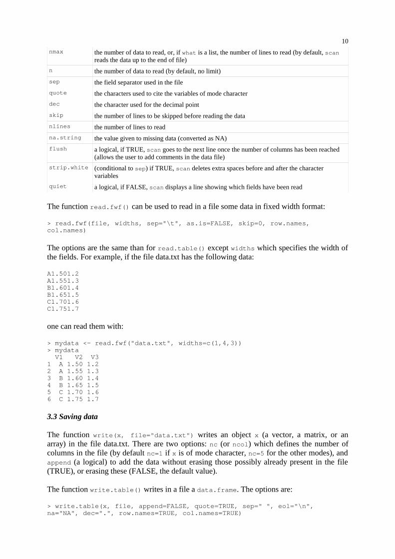
10

nmax the number of data to read, or, if what is a list, the number of lines to read (by default, scanreads the data up to the end of file)

n the number of data to read (by default, no limit)

sep the field separator used in the file

quote the characters used to cite the variables of mode character

dec the character used for the decimal point

skip the number of lines to be skipped before reading the data

nlines the number of lines to read

na.string the value given to missing data (converted as NA)

flush a logical, if TRUE, scan goes to the next line once the number of columns has been reached(allows the user to add comments in the data file)

strip.white (conditional to sep) if TRUE, scan deletes extra spaces before and after the charactervariables

quiet a logical, if FALSE, scan displays a line showing which fields have been read

The function read.fwf() can be used to read in a file some data in fixed width format:

> read.fwf(file, widths, sep="\t", as.is=FALSE, skip=0, row.names,col.names)

The options are the same than for read.table() except widths which specifies the width ofthe fields. For example, if the file data.txt has the following data:

A1.501.2A1.551.3B1.601.4B1.651.5C1.701.6C1.751.7

one can read them with:

> mydata <- read.fwf("data.txt", widths=c(1,4,3))> mydata V1 V2 V31 A 1.50 1.22 A 1.55 1.33 B 1.60 1.44 B 1.65 1.55 C 1.70 1.66 C 1.75 1.7

3.3 Saving data

The function write(x, file="data.txt") writes an object x (a vector, a matrix, or anarray) in the file data.txt. There are two options: nc (or ncol) which defines the number ofcolumns in the file (by default nc=1 if x is of mode character, nc=5 for the other modes), andappend (a logical) to add the data without erasing those possibly already present in the file(TRUE), or erasing these (FALSE, the default value).

The function write.table() writes in a file a data.frame. The options are:

> write.table(x, file, append=FALSE, quote=TRUE, sep=" ", eol="\n",na="NA", dec=".", row.names=TRUE, col.names=TRUE)

11

sep the field separator used in the file

col.names a logical indicating whether the names of the columns are written in the file

row.names id. for the names of the lines

quote a logical or a numeric vector; if TRUE, the variables of mode character are quoted with ""; if anumeric vector, its elements gives the indices of the columns to be quoted with "". In both cases,the names of the lines and of the columns are also quoted with "" if they are written.

dec the character to be used for the decimal point

na the character to be used for missing data

eol the character to be used at the end of each line ("\n" is a carriage-return)

To record a group of objects in a binary form, we can use the function save(x, y, z,

file="Mystuff.RData"). To ease the transfert of data between different machines, theoption ascii=TRUE can be used. The data (which are now called image) can be loaded later inmemory with load("Mystuff.RData"). The function save.image() is a short-cut forsave(list=ls(all=TRUE), file=".RData").

3.4 Generating data

3.4.1 Regular sequencesA regular sequence of integers, for example from 1 to 30, can be generated with:

> x <- 1:30

The resulting vector x has 30 éléments. The operator ‘:’ has priority on the arithmeticoperators within an expression:

> 1:10-1 [1] 0 1 2 3 4 5 6 7 8 9> 1:(10-1)[1] 1 2 3 4 5 6 7 8 9

The function seq() can generate sequences oe real numbers as follows:

> seq(1, 5, 0.5)[1] 1.0 1.5 2.0 2.5 3.0 3.5 4.0 4.5 5.0

where the first number indicates the start of the sequence, the second one the end, and thethird one the increment to be used to generate the sequence. One can use also:

> seq(length=9, from=1, to=5)[1] 1.0 1.5 2.0 2.5 3.0 3.5 4.0 4.5 5.0

It is also possible to type directly the values using the function c() :

> c(1, 1.5, 2, 2.5, 3, 3.5, 4, 4.5, 5)[1] 1.0 1.5 2.0 2.5 3.0 3.5 4.0 4.5 5.0

which gives exactly the same result, but is obviously longer. We shall see late that thefunction c() is more useful in other situations. The function rep() creates a vector withelements all identical:

> rep(1, 30) [1] 1 1 1 1 1 1 1 1 1 1 1 1 1 1 1 1 1 1 1 1 1 1 1 1 1 1 1 1 1 1

12

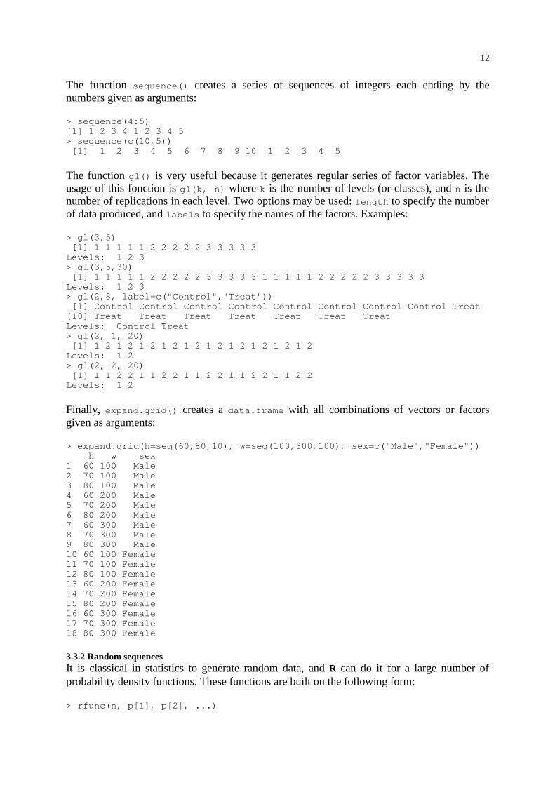
The function sequence() creates a series of sequences of integers each ending by thenumbers given as arguments:

> sequence(4:5)[1] 1 2 3 4 1 2 3 4 5> sequence(c(10,5)) [1] 1 2 3 4 5 6 7 8 9 10 1 2 3 4 5

The function gl() is very useful because it generates regular series of factor variables. Theusage of this fonction is gl(k, n) where k is the number of levels (or classes), and n is thenumber of replications in each level. Two options may be used: length to specify the numberof data produced, and labels to specify the names of the factors. Examples:

> gl(3,5) [1] 1 1 1 1 1 2 2 2 2 2 3 3 3 3 3Levels: 1 2 3> gl(3,5,30) [1] 1 1 1 1 1 2 2 2 2 2 3 3 3 3 3 1 1 1 1 1 2 2 2 2 2 3 3 3 3 3Levels: 1 2 3> gl(2,8, label=c("Control","Treat")) [1] Control Control Control Control Control Control Control Control Treat[10] Treat Treat Treat Treat Treat Treat TreatLevels: Control Treat> gl(2, 1, 20) [1] 1 2 1 2 1 2 1 2 1 2 1 2 1 2 1 2 1 2 1 2Levels: 1 2> gl(2, 2, 20) [1] 1 1 2 2 1 1 2 2 1 1 2 2 1 1 2 2 1 1 2 2Levels: 1 2

Finally, expand.grid() creates a data.frame with all combinations of vectors or factorsgiven as arguments:

> expand.grid(h=seq(60,80,10), w=seq(100,300,100), sex=c("Male","Female")) h w sex1 60 100 Male2 70 100 Male3 80 100 Male4 60 200 Male5 70 200 Male6 80 200 Male7 60 300 Male8 70 300 Male9 80 300 Male10 60 100 Female11 70 100 Female12 80 100 Female13 60 200 Female14 70 200 Female15 80 200 Female16 60 300 Female17 70 300 Female18 80 300 Female

3.3.2 Random sequencesIt is classical in statistics to generate random data, and R can do it for a large number ofprobability density functions. These functions are built on the following form:

> rfunc(n, p[1], p[2], ...)

13

whre func indicates the law of probability, n the number of data to generate and p[1], p[2],... are the values for the parameters of the law. The following table gives the details for eachlaw, and the possible default values (if none default value is indicated, this means that theparameter must be specified by the user).

loi commande

Gaussian (normal) rnorm(n, mean=0, sd=1)

exponential rexp(n, rate=1)

gamma rgamma(n, shape, scale=1)

Poisson rpois(n, lambda)

Weibull rweibull(n, shape, scale=1)

Cauchy rcauchy(n, location=0, scale=1)

beta rbeta(n, shape1, shape2)

‘Student’ (t) rt(n, df)

Fisher (F) rf(n, df1, df2)

Pearson (χ2) rchisq(n, df)

binomial rbinom(n, size, prob)

geometric rgeom(n, prob)

hypergeometric rhyper(nn, m, n, k)

logistic rlogis(n, location=0, scale=1)

lognormal rlnorm(n, meanlog=0, sdlog=1)

negative binomial rnbinom(n, size, prob)

uniform runif(n, min=0, max=1)

Wilcoxon’s statistics rwilcox(nn, m, n), rsignrank(nn, n)

Note all these functions can be used by replacing the letter r with d, p or q to get, respectively,the probability density (dfunc(x)), the cumulative probability density (pfunc(x)), and thevalue of quantile (qfunc(p), with 0 < p < 1).

3.4 Manipulating objects

3.4.1 Accessing a particular value of an objectTo access, for example, the third value of a vector x, we just type x[3]. If x is a matrix or adata.frame, the value of the ith line and jth column is accessed with x[i,j]. To change allvalues of the third column, we can type:

> x[,3] <- 10.2

This indexing system is easily generalised to arrays, with as many indices as the number ofdimensions of the array (for example, a three dimensional array: x[i,j,k], x[,,3], ...). It isuseful to keep in mind that indexing is made with straight brackets [], whereas parenthesesare used for the arguments of a function:

> x(1)Error: couldn’t find function "x"

Indexing can be used to suppress one or several lines or columns. For examples, x[-1,] willsuppress the first line, or x[-c(1,15),] will do the same for the 1st and 15th lines.

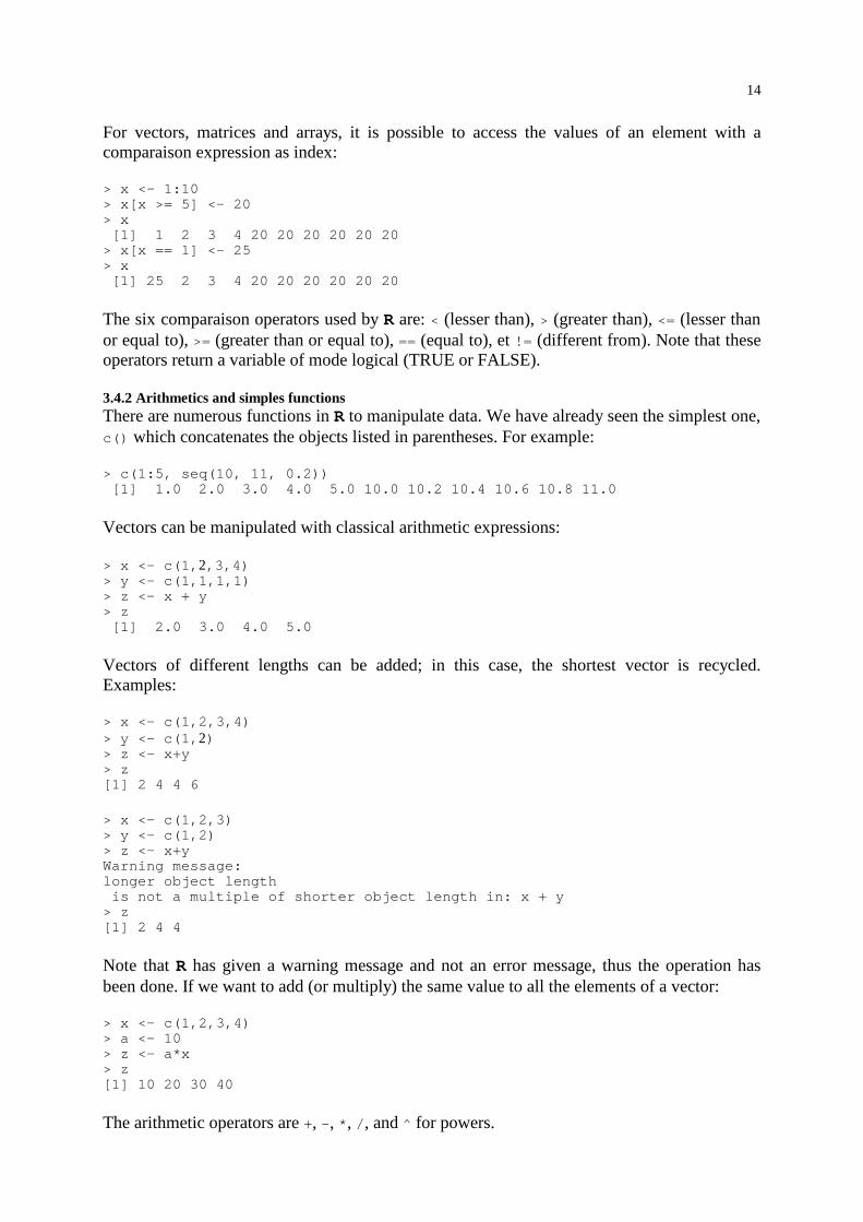
14

For vectors, matrices and arrays, it is possible to access the values of an element with acomparaison expression as index:

> x <- 1:10> x[x >= 5] <- 20> x [1] 1 2 3 4 20 20 20 20 20 20> x[x == 1] <- 25> x [1] 25 2 3 4 20 20 20 20 20 20

The six comparaison operators used by R are: < (lesser than), > (greater than), <= (lesser thanor equal to), >= (greater than or equal to), == (equal to), et != (different from). Note that theseoperators return a variable of mode logical (TRUE or FALSE).

3.4.2 Arithmetics and simples functionsThere are numerous functions in R to manipulate data. We have already seen the simplest one,c() which concatenates the objects listed in parentheses. For example:

> c(1:5, seq(10, 11, 0.2)) [1] 1.0 2.0 3.0 4.0 5.0 10.0 10.2 10.4 10.6 10.8 11.0

Vectors can be manipulated with classical arithmetic expressions:

> x <- c(1,2,3,4)> y <- c(1,1,1,1)> z <- x + y> z [1] 2.0 3.0 4.0 5.0

Vectors of different lengths can be added; in this case, the shortest vector is recycled.Examples:

> x <- c(1,2,3,4)> y <- c(1,2)> z <- x+y> z[1] 2 4 4 6

> x <- c(1,2,3)> y <- c(1,2)> z <- x+yWarning message: longer object length is not a multiple of shorter object length in: x + y> z[1] 2 4 4

Note that R has given a warning message and not an error message, thus the operation hasbeen done. If we want to add (or multiply) the same value to all the elements of a vector:

> x <- c(1,2,3,4)> a <- 10> z <- a*x> z[1] 10 20 30 40

The arithmetic operators are +, -, *, /, and ^ for powers.

15

Two other useful operators are x %% y for “x modulo y”, and x %/% y for integer divisions(returns the integer part of the division of x by y).

The functions available in R are too many to be listed here. One can find all basicmathematical functions (log, exp, log10, log2, sin, cos, tan, asin, acos, atan, abs, sqrt,...), special functions (gamma, digamma, beta, besselI, ...), as well as diverse functions usefulin statistics. Some of these functions are detailed in the following table.

sum(x) sum of the elements of x

prod(x) product of the elements of x

max(x) maximum of the elements of x

min(x) minimum of the elements of x

which.max(x) returns the index of the greatest element of x

which.min(x) returns the index of the smallest element of x

range(x) has the same result than c(min(x),max(x))

length(x) number of elements in x

mean(x) mean of the elements of x

median(x) median of the elements of x

var(x) ou cov(x) variance of the elements of x (calculated on n – 1); if x is a matrix or a data.frame,the variance-covariance matrix is calculated

cor(x) correlation matrix of x if it is a matrix or a data.frame (1 if x is a vector)

var(x,y) oucov(x,y)

covariance between x and y, or between the columns of x and the columns of y if theyare matrices or data.frames

cor(x,y) linear correlation between x and y, or correlation matrix if they are matrices ordata.frames

These functions return a single value (thus a vector of length one), except range() whichreturns a vector of length two, and var(), cov() and cor() which may return a matrix. Thefollowing functions return more complex results.

round(x,n) rounds the elements of x to n decimals

rev(x) reverses the elements of x

sort(x) sorts the elements of x in increasing order; to sort in decreasing order: rev(sort(x))

rank(x) ranks of the elements of x

log(x,base) computes the logarithm of x with base base

pmin(x,y,...) a vector which ith element is the minimum of x[i], y[i], ...

pmax(x,y,...) id. for the maximum

cumsum(x) a vector which ith element is the sum from x[1] to x[i]

cumprod(x) id. for the product

cummin(x) id. for the minimum

cummax(x) id. for the maximum

match(x,y) returns a vector of same length than x with the elements of x which are in y (else NA)

which(x==a)

which(x!=a)

...

returns a vector of the indices of x if the comparison operation is true (TRUE), i.e. thevalues of i for which x[i]==a (or x!=a; the argument of this function must be a variable ofmode logical)

16

choose(n,k) computes the combinations of k events among n repetitions = n!/[(n – k)!k!]

na.omit(x) suppresses the observations with missing data (NA) (suppresses the corresponding line if xis a matrix or a data.frame)

na.fail(x) returns an error message if x contains NA(s)

table(x) returns a table with the numbers of the differents values of x (typically for integers orfactors)

subset(x,...) returns a selection of x with respect to criteria (...) depending on the mode of x (typicallycomparisons: x$V1 < 10); if x is a data.frame, the option select allows the user toidentify variables to be kept (or dropped using a minus sign -)

3.4.3 Matrix computationR has facilities for matric computation and manipulation. A matrix can be created with thefunction matrix():

> matrix(data=5, nr=2, nc=2) [,1] [,2][1,] 5 5[2,] 5 5> matrix(1:6, nr=2, nc=3) [,1] [,2] [,3][1,] 1 3 5[2,] 2 4 6

The functions rbind() and cbind() bind matrices with respect to the lines or the columns,respectively:

> m1 <- matrix(data=1, nr=2, nc=2)> m2 <- matrix(data=2, nr=2, nc=2)> rbind(m1,m2) [,1] [,2][1,] 1 1[2,] 1 1[3,] 2 2[4,] 2 2> cbind(m1,m2) [,1] [,2] [,3] [,4][1,] 1 1 2 2[2,] 1 1 2 2

The operator for the product of two matrices is ‘%*%’. For example, considering the twomatrices m1 and m2 above:

> rbind(m1,m2) %*% cbind(m1,m2) [,1] [,2] [,3] [,4][1,] 2 2 4 4[2,] 2 2 4 4[3,] 4 4 8 8[4,] 4 4 8 8> cbind(m1,m2) %*% rbind(m1,m2) [,1] [,2][1,] 10 10[2,] 10 10

The transposition of a matrix is done with the function t(); this function also with adata.frame.

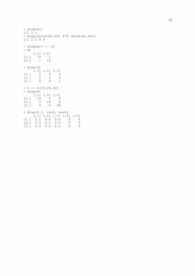
The function diag() can be used to extract or modify the diagonal of a matrix, or to builddiagonal matrix.

17

> diag(m1)[1] 1 1> diag(rbind(m1,m2) %*% cbind(m1,m2))[1] 2 2 8 8

> diag(m1) <- 10> m1 [,1] [,2][1,] 10 1[2,] 1 10

> diag(3) [,1] [,2] [,3][1,] 1 0 0[2,] 0 1 0[3,] 0 0 1

> v <- c(10,20,30)> diag(v) [,1] [,2] [,3][1,] 10 0 0[2,] 0 20 0[3,] 0 0 30

> diag(2.1, nr=3, nc=5) [,1] [,2] [,3] [,4] [,5][1,] 2.1 0.0 0.0 0 0[2,] 0.0 2.1 0.0 0 0[3,] 0.0 0.0 2.1 0 0

18

4 Graphics with R

R offers a remarkable variety of graphics. To get an idea, one can type demo(graphics). It isnot possible to detail here the possibilities of R in terms of graphics, particularly each graphicfunction has a large number of options making the production of graphics very flexible. I willfirst give a few details on how to manage graphic windows.

4.1 Managing graphic windows

4.1.1 Opening several graphic windowsWhen a graphic function is typed, a graphic window is open with the graph required. It ispossible to open another window by typing:

> x11()

The window so open becomes the active window, and the subsequent graphs will be displayedon it. To know the graphic windows which are currently open:

> dev.list()windows windows 2 3

The figures displayed under windows are the numbers of the windows which can be used tochange the active window:

> dev.set(2)windows 2

4.1.2 Partitioning a graphic windowThe function split.screen() partitions the active graphic window. For instance,split.screen(c(1,2)) divide the window in two parts which can be selected withscreen(1) or screen(2); erase.screen() erases the last drawn graph.

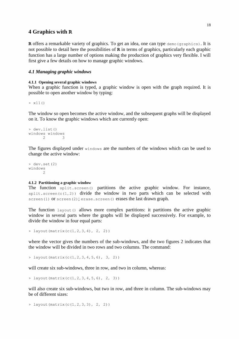
The function layout() allows more complex partitions: it partitions the active graphicwindow in several parts where the graphs will be displayed successively. For example, todivide the window in four equal parts:

> layout(matrix(c(1,2,3,4), 2, 2))

where the vector gives the numbers of the sub-windows, and the two figures 2 indicates thatthe window will be divided in two rows and two columns. The command:

> layout(matrix(c(1,2,3,4,5,6), 3, 2))

will create six sub-windows, three in row, and two in column, whereas:

> layout(matrix(c(1,2,3,4,5,6), 2, 3))

will also create six sub-windows, but two in row, and three in column. The sub-windows maybe of different sizes:

> layout(matrix(c(1,2,3,3), 2, 2))

19

will open two sub-windows in row in the left half of the window, and a third sub-window inthe right half. Finally, to create an inlet in a graphic:

> layout(matrix(c(1,1,2,1), 2, 2), c(3,1), c(1,3))

the vectors c(3,1) and c(1,3) giving the relative dimensions of the sub-windows.

To visualize the partition created by layout() before drawing the graphs, we can use thefunction layout.show(2), if, for example, two sub-windows have been defined.

4.2 Graphic functions

Here is a brief overview of the graphics functions in R.

plot(x) plot of the values of x (on the y-axis) ordered on the x-axis

plot(x,y) bivariate plot of x (on the x-axis) and y (on the y-axis)

sunflowerplot(x,y) id. than plot() but the points with similar coordinates are drawn as flowers whichpetal number represents the number of points

piechart(x) circular pie-chart

boxplot(x) “box-and-whiskers” plot

stripplot(x) plot the values of x on a line (an alternative to boxplot()for small sample sizes)

coplot(x~y|z) bivariate plot of x and y for each value of z (if z is a factor)

interaction.plot(f1,f2,x)

if f1 and f2 are factors, plots the means of y (on the y-axis) with respect to the valuesof f1 (on the x-axis) and of f2 (different curves) ; the option fun= allows to choosethe summary statistic of y (by default fun=mean)

matplot(x,y) bivariate plot of the first column of x vs. the first one of y, the second one of x vs. thesecond one of y, etc.

dotplot(x) if x is a data.frame, plots a Cleveland dot plot (stacked plots line-by-line andcolumn-by-column)

pairs(x) if x is a matrix or a data.frame, draws all possible bivariate plots between thecolumns of x

plot.ts(x) if x is an object of class ts, plot of x with respect to time, x may be multivariate butthe series must have the same frequency and dates

ts.plot(x) id. but if x is multivariate the series may have different dates and must have the samefrequency3

hist(x) histogram of the frequencies of x

barplot(x) histogram of the values of x

qqnorm(x) quantiles of x with respect to the values expected under a normal law

qqplot(x,y) quantiles of y with respect to the quantiles of x

contour(x,y,z) creates a contour plot (data are interpolated to draw the curves), x and y must bevectors and z must be a matrix so that dim(z)=c(length(x),length(y))

image(x,y,z) id. but with colours (actual data are plotted)

persp(x,y,z) id. but in 3-D (actual data are plotted)

For each function, the options may be found with the on-line help in R. Some of these optionsare identical for several graphic functions; here are the main ones (with their possible defaultvalues):

3 The function ts.plot() is in the package ts and not in base as for the other graphic functions listed in thetable (see § 5 for details on packages in R).

20

add=FALSE if TRUE superposes the plot on the previous one (if it exists)axes=TRUE if FALSE does not draw the axestype="p" specifies the type of plot, "p": points, "l": lines, "b": points connected by

lines, "o": id. but the lines are over the points, "h": vertical lines , "s": steps,the data are represented by the top of the vertical lines, "S": id. but the dataare represented by the bottom of the vertical lines.

xlab=, ylab= annotates the axes, must be variables of mode character (either a charactervariable, or a string within "")

main= main title, must be a variable of mode charactersub= sub-title (written in a smaller font)

4.3 Low-level plotting commands

R has a set of graphic functions which affect an already existing graph: they are called low-level plotting commands. Here are the main ones:

points(x,y) adds points (the option type= can be used)

lines(x,y) id. but with lines

text(x,y,labels,...) adds text given by labels at coordinates (x, y); a typical usage is:plot(x,y,type="n"); text(x,y,names)

segments(x0,y0,x1,y1) draws a line from point (x0,y0) to point (x1,y1)

arrows(x0,y0,x1,y1,angle=30, code=2)

id. with an arrow at point (x0,y0) if code=2, at point (x1,y1) if code=1, or at bothpoints if code=3; angle controls the angle from the shaft of the arrow to theedge of the arrow head

abline(a,b) draws a line of slope b and intercept a

abline(h=y) draws a horizontal line at ordinate y

abline(v=x) draws a vertical line at abcissa x

abline(lm.obj) draws the regression line given by lm.obj (see § 5)

rect(x1,y1,x2,y2) draws a rectangle which left, right, bottom, and top limits are x1, x2, y1, and y2,respectively

polygon(x,y) draws a polygon linking the points with coordinates given x and y

legend(x,y,legend) adds the legend at the point (x,y) with symbols given by legend

title() adds a title and optionally a sub-title

axis(side,vect) adds an axis at the bottom (side=1), on the left (2), at the top (3), or on the right(4); vect (optional) gives the abcissa (or ordinates) where tick-marks are drawn

rug(x) draws the data x on the x-axis as small vertical lines

locator(n, type="n",...)

returns the coordinates (x,y) after the user has clicked n times on the plot with themouse; also draws symbols (type="p") or lines (type="l") with respect tooptional graphic parameters (...); by default nothing is drawn (type="n")

Note the possibility to add mathematical expressions on a plot with text(x, y,

expression(...)), where the function expression() transforms its argument in amathematical equation according to a coding used in the type-setting TeX. For example,text(x, y, expression(Uk[37]==over(1, 1+e^{-epsilon*(T-theta)}))) will display,on the plot, the following equation at point of coordinates (x,y):

Uk37=1

1Ae� ��� T �����

21

To include in an expression a variable we can use the function substitute() together withthe function as.expression(); for example to include a value of R2 (previously computedand stored in an object named Rsquared):

> text(x, y, as.expression(substitute(R^2==r, list(r=Rsquared))))

will display on the plot at the point of coordinates (x,y):

R2 = 0.9856298

To display only three decimals, we can modify the code as follows:

> text(x, y, as.expression(substitute(R^2==r, list(r=round(Rsquared,3)))))

which will result in:

R2 = 0.986

Finally, to write the R in italics (as are the mathematical conventions):

>text(x, y, as.expression(substitute(italic(R)^2==r,list(r=round(Rsquared,3)))))

R2 = 0.986

4.4 Graphic parameters

In addition to low-level plotting commands, the presentation of graphics can be improvedwith graphic parameters. They can be used either as options of graphic functions (but it doesnot work for all), oe with the function par() to change permanently the graphic parameters,i.e. the subsequent plots with respect to the parameters specified by the user. For instance,l’instruction suivante:

> par(bg="yellow")

will draw all subsequent plots with a yellow background. There are 68 graphic parameters,some of them have very close functions. The exhaustive list of graphic parameters can be readwith ?par; I will limit the following table to the most usual ones.

adj controls text justification (0 left-justified, 0.5 centered, 1 right-justified)

bg specifies the colour of the background (e.g.: bg="red", bg="blue", ... the list of the 657 availablecolours is displayed with colors())

bty controls the type of box drawn around the plot, allowed values are: "o", "l", "7", "c", "u" or "]"(the box looks like the corresponding character); if bty="n" the box is not drawn

cex a value controling the size of texts and symbols with respect to the default; the following parametershave the same control for numbers on the axes, cex.axis, annotations on the axes, cex.lab, thetitle, cex.title, and the sub-title, cex.sub

col controls the colour of symbols; as for cex there are: col.axis, col.lab, col.title, col.sub

font an integer which controls the style of text (0: normal, 1: italics, 2: bold, 3: bold italics); as for cexthere are: font.axis, font.lab, font.title, font.sub

22

las an integer which controls the orientation of annotations on the axes (0: parallel to the axes, 1:horizontal, 2: perpendicular to the axes, 3: vertical)

lty controls the type of lines, can be an integer (1: solid, 2: dashed, 3: dotted, 4: dotdash, 5: longdash, 6:twodash), or a string of up to eight characters (between "0" and "9") which specifies alternatively thelength, in points or pixels, of the drawn elements and the blanks, for example lty="44" will have thesame effet than lty=2

lwd a numeric which controls the width of lines

mar a vector of 4 numeric values which control the space between the axes and the border of the figure ofthe form c(bottom, left, top, right), the default values are c(5.1, 4.1, 4.1, 2.1)

mfcol a vector of the form c(nr,nc) which partitions the graphic window as a matrix of nr lines and nccolumns, the plots are then drawn in columns (cf. § 4.1.2)

mfrow id. but the plots are drawn in rows (cf. § 4.1.2)

pch controls the type of symbol, either an integer between 1 and 25, or any single character within ""

ps an integer which controls the size in points of texts and symbols

pty a character which specifies the type of the plotting region, "s": square, "m": maximal

tck a value which specifies the length of tick-marks on the axes as a fraction of the smallest of the widthor height of the plot; if tck=1 a grid is drawn

tcl a value which specifies the length of tick-marks on the axes as a fraction of the height of a line of text(by default tcl=-0.5)

xaxt if xaxt="n" the x-axis is set but not drawn (useful in conjonction with axis(side=1, ...))

yaxt if yaxt="n" the y-axis is set but not drawn (useful in conjonction with axis(side=2, ...))

23

5 Statistical analyses with R

Even more than for graphics, it is impossible here to go in the details of the possibilitiesoffered by R with respect to statistical analyses. A wide range of functions is available in thebase package and in others distributed with base.

Several contributed packages increase the potentialities of R. They are distributed separatelyand must be loaded in memory to be used by R. An exhaustive list of the contributedpackages, together with their descriptions, is at the following URL: http://cran.r-project.org/src/contrib/PACKAGES.html. Among the most remarkable ones, there are:

gee generalised estimating equations;multiv multivariate analyses, includes correspondance analysis

(by contrats to mva which is distributed with base) ;nlme linear and nonlinear models with mixed-effects;survival5 survival analyses;tree trees and classification;tseries time-series analyses

(has more methods than ts which is distributed with base).

Jim K. Lindsey distributes on his site (http://alpha.luc.ac.be/~jlindsey/rcode.html) severalinteresting packages:

dna manipulation of molecular sequences (includes the ports of ClustalW and of flip)gnlm nonlinear generalized models;stable probability functions and generalized regressions for stable distributions;growth models for normal repeated measures;repeated models for non-normal repeated measures;event models and procedures for historical processes (branching, Poisson, ...)rmutil tools for nonlinear regressions and repeated measures.

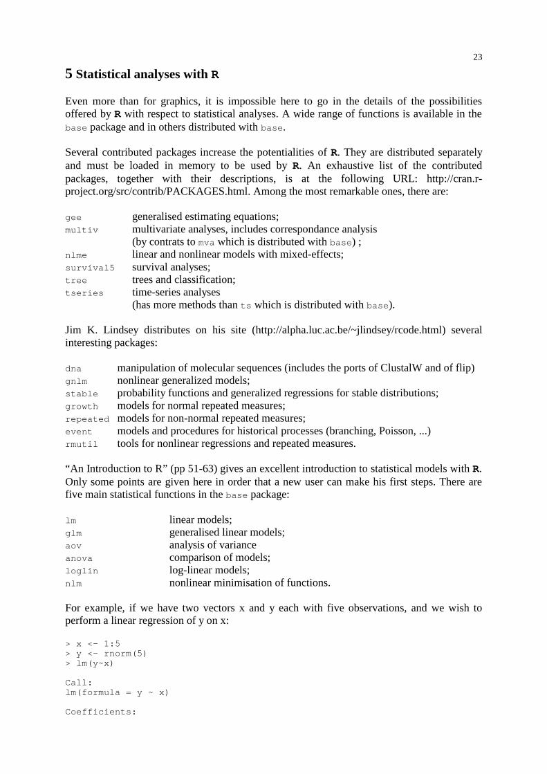
“An Introduction to R” (pp 51-63) gives an excellent introduction to statistical models with R.Only some points are given here in order that a new user can make his first steps. There arefive main statistical functions in the base package:

lm linear models;glm generalised linear models;aov analysis of variance anova comparison of models;loglin log-linear models;nlm nonlinear minimisation of functions.

For example, if we have two vectors x and y each with five observations, and we wish toperform a linear regression of y on x:

> x <- 1:5> y <- rnorm(5)> lm(y~x)

Call:lm(formula = y ~ x)

Coefficients:

24(Intercept) x 0.2252 0.1809

As for any function in R, the result of lm(y~x) can be copied in an object:

> mymodel <- lm(y~x)

if we type mymodel, the display will be the same than previously. Several functions allow theuser to display details relative to a statistical model, among the useful ones summary()

displays details on the results of a model fitting procedure (statistical tests, ...), residuals()displays the regression residuals, predict() displays the values predicted by the model, andcoef() displays a vector with the parameter estimates.

> summary(mymodel)

Call:lm(formula = y ~ x)

Residuals: 1 2 3 4 5 1.0070 -1.0711 -0.2299 -0.3550 0.6490

Coefficients: Estimate Std. Error t value Pr(>|t|)(Intercept) 0.2252 1.0062 0.224 0.837x 0.1809 0.3034 0.596 0.593

Residual standard error: 0.9594 on 3 degrees of freedomMultiple R-Squared: 0.1059, Adjusted R-squared: -0.1921 F-statistic: 0.3555 on 1 and 3 degrees of freedom, p-value: 0.593

> residuals(mymodel) 1 2 3 4 5 1.0070047 -1.0710587 -0.2299374 -0.3549681 0.6489594

> predict(mymodel) 1 2 3 4 5 0.4061329 0.5870257 0.7679186 0.9488115 1.1297044

> coef(mymodel)(Intercept) x 0.2252400 0.1808929

It may be useful to use these values in subsequent computations, for instance, to computepredicted values with by a model for new data:

> a <- coef(mymodel)[1]> b <- coef(mymodel)[2]> newdata <- c(11, 13, 18)> a + b*newdata[1] 2.215062 2.576847 3.481312

To list the elements in the results of an analysis, we can use the function names(); in fact, thisfunction may be used with any object in R.

> names(mymodel) [1] "coefficients" "residuals" "effects" "rank" [5] "fitted.values" "assign" "qr" "df.residual" [9] "xlevels" "call" "terms" "model"

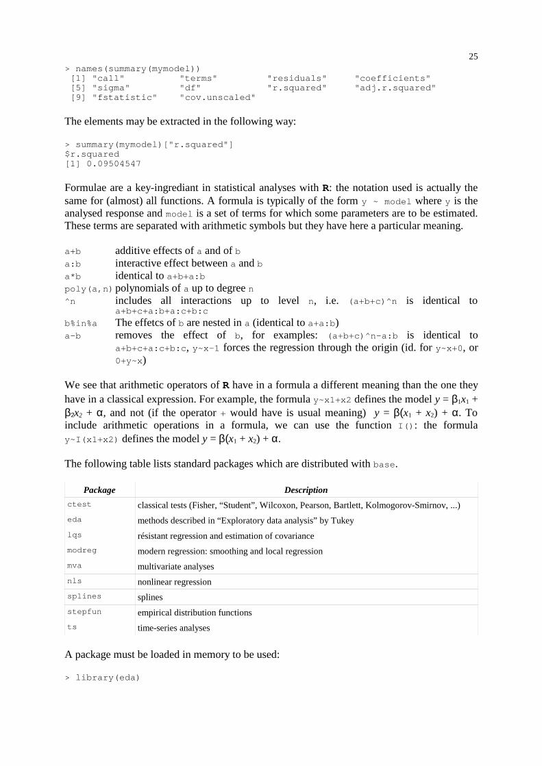
25> names(summary(mymodel)) [1] "call" "terms" "residuals" "coefficients" [5] "sigma" "df" "r.squared" "adj.r.squared" [9] "fstatistic" "cov.unscaled"

The elements may be extracted in the following way:

> summary(mymodel)["r.squared"]$r.squared[1] 0.09504547

Formulae are a key-ingrediant in statistical analyses with R: the notation used is actually thesame for (almost) all functions. A formula is typically of the form y ~ model where y is theanalysed response and model is a set of terms for which some parameters are to be estimated.These terms are separated with arithmetic symbols but they have here a particular meaning.

a+b additive effects of a and of ba:b interactive effect between a and ba*b identical to a+b+a:bpoly(a,n)polynomials of a up to degree n^n includes all interactions up to level n, i.e. (a+b+c)^n is identical to

a+b+c+a:b+a:c+b:c

b%in%a The effetcs of b are nested in a (identical to a+a:b)a-b removes the effect of b, for examples: (a+b+c)^n-a:b is identical to

a+b+c+a:c+b:c, y~x-1 forces the regression through the origin (id. for y~x+0, or0+y~x)

We see that arithmetic operators of R have in a formula a different meaning than the one theyhave in a classical expression. For example, the formula y~x1+x2 defines the model y = β1x1 +β2x2 + α, and not (if the operator + would have is usual meaning) y = β(x1 + x2) + α. Toinclude arithmetic operations in a formula, we can use the function I(): the formulay~I(x1+x2) defines the model y = β(x1 + x2) + α.

The following table lists standard packages which are distributed with base.

Package Description

ctest classical tests (Fisher, “Student”, Wilcoxon, Pearson, Bartlett, Kolmogorov-Smirnov, ...)

eda methods described in “Exploratory data analysis” by Tukey

lqs résistant regression and estimation of covariance

modreg modern regression: smoothing and local regression

mva multivariate analyses

nls nonlinear regression

splines splines

stepfun empirical distribution functions

ts time-series analyses

A package must be loaded in memory to be used:

> library(eda)

26

6 The programming language R

6.1 Loops and conditional executions

An advantage of R compared to softwares with pull-down menus is the possibility to programsimply a series of analyses which will be executed successively. Let us consider a fewexamples to get an idea.

Suppose we have a vector x, and for each element of x with the value b, we want to give thevalue 0 to another variable y, else 1. We first create a vector y of the same length than x:

> y <- numeric(length(x))> for (i in 1:length(x)) if (x[i] == b) y[i] <- 0 else y[i] <- 1

Several instructions can be executed if they are placed within braces:

> for (i in 1:length(x))> {> y[i] <- 0...> }

> if (x[i] == b)> {> y[i] <- 0...> }

Another possible situation is to execute an instruction as long as a condition is true:

> while (myfun > minimum)> {...> }

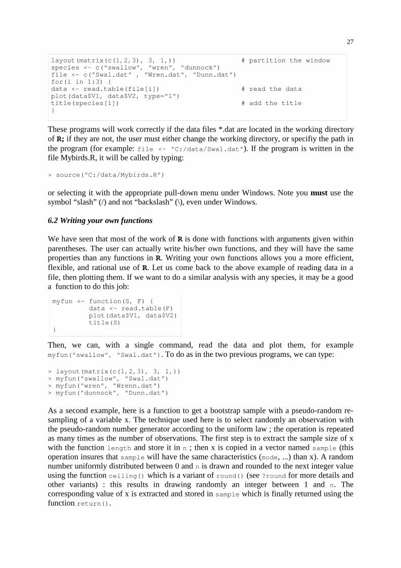
Typically, an R program is written in a file saved in ASCII format and named with theextension .R. In the following example, we want to do the same plot for three differentspecies, the data being in three distinct files, the file names and species names are so used asvariables. The first command partitions the graphic window in three arranged as rows.

The character # is used to add comments in a program, R then goes to the next line. Note thatthere are no brackets "" around file in the function read.table() since it is a variable ofmode character. The command title adds a title on a plot already displayed. A variant ofthis program is given by:

layout(matrix(c(1,2,3), 3, 1,)) # partition the windowfor(i in 1:3) {if (i==1) { file <- "Swal.dat"; species <- "swallow" }if (i==2) { file <- "Wren.dat"; species <- "wren" }if (i==3) { file <- "Dunn.dat"; species <- "dunnock" }data <- read.table(file) # read the dataplot(data$V1, data$V2, type="l")title(species) # adds the title}

27

These programs will work correctly if the data files *.dat are located in the working directoryof R; if they are not, the user must either change the working directory, or specifiy the path inthe program (for example: file <- "C:/data/Swal.dat"). If the program is written in thefile Mybirds.R, it will be called by typing:

> source("C:/data/Mybirds.R")

or selecting it with the appropriate pull-down menu under Windows. Note you must use thesymbol “slash” (/) and not “backslash” (\), even under Windows.

6.2 Writing your own functions

We have seen that most of the work of R is done with functions with arguments given withinparentheses. The user can actually write his/her own functions, and they will have the sameproperties than any functions in R. Writing your own functions allows you a more efficient,flexible, and rational use of R. Let us come back to the above example of reading data in afile, then plotting them. If we want to do a similar analysis with any species, it may be a gooda function to do this job:

Then, we can, with a single command, read the data and plot them, for examplemyfun("swallow", "Swal.dat"). To do as in the two previous programs, we can type:

> layout(matrix(c(1,2,3), 3, 1,))> myfun("swallow", "Swal.dat")> myfun("wren", "Wrenn.dat")> myfun("dunnock", "Dunn.dat")

As a second example, here is a function to get a bootstrap sample with a pseudo-random re-sampling of a variable x. The technique used here is to select randomly an observation withthe pseudo-random number generator according to the uniform law ; the operation is repeatedas many times as the number of observations. The first step is to extract the sample size of xwith the function length and store it in n ; then x is copied in a vector named sample (thisoperation insures that sample will have the same characteristics (mode, ...) than x). A randomnumber uniformly distributed between 0 and n is drawn and rounded to the next integer valueusing the function ceiling() which is a variant of round() (see ?round for more details andother variants) : this results in drawing randomly an integer between 1 and n. Thecorresponding value of x is extracted and stored in sample which is finally returned using thefunction return().

myfun <- function(S, F) { data <- read.table(F) plot(data$V1, data$V2) title(S)}

layout(matrix(c(1,2,3), 3, 1,)) # partition the windowspecies <- c("swallow", "wren", "dunnock")file <- c("Swal.dat" , "Wren.dat", "Dunn.dat")for(i in 1:3) {data <- read.table(file[i]) # read the dataplot(data$V1, data$V2, type="l")title(species[i]) # add the title}

28

Thus, one can, with a few, relatively simple lines of code, program a method of bootstrap withR. This function can then be called by a second function to compute the standard-error of anestimated parameter, for instance the mean:

Note the value by default of the argument rep, so that it can be omitted if we are satisfied with500 réplications. The two following commands will thus have the same effect:

> meanboot(x)> meanboot(x, rep=500)

If we want to increase the number of replications, we can do, for example:

> meanboot(x, rep=5000)

The use of default values in the definition of a function is, of course, very useful and adds tothe flexibility of the system.

The last example of function is not purely statistical, but it illustrates well the flexibility of R.Consider we wish to study the behaviour of a nonlinear model: Ricker’s model defined by:

N t � 1=N t exp�r�1 BN t

K ��This model is widely used in population dynamics, particularly of fish. We want, using afunction, simulate this model with respect to the growth rate r and the initial number in thepopulation N0 (the carrying capacity K is often taken equal to 1 and this value will be taken asdefault); the results will be displayed as a plot of numbers with respect to time. We will addan option to allow the user to display only the numbers in the last time steps (by default allresults will be plotted). The function below can do this numerical analysis of Ricker’s model.

bootsamp <- function(x) { n <- length(x) sample <- x for (i in 1:n) { u <- ceiling(runif(1, 0, n)) sample[i] <- x[u] } return(sample)}

meanboot <- function(x, rep=500) { M <- numeric(rep) for (i in 1:rep) M[i] <- mean(bootsamp(x)) print(var(M))}

ricker <- function(nzero, r, K=1, time=100, from=0, to=time) { N <- numeric(time+1) N[1] <- nzero for (i in 1:time) N[i+1] <- N[i]*exp(r*(1 - N[i]/K)) Time <- 0:time plot(Time, N, type="l", xlim=c(from,to))}

29

Try it yourself with:

> layout(matrix(1:3, 3, 1))> ricker(0.1, 1); title("r = 1")> ricker(0.1, 2); title("r = 2")> ricker(0.1, 3); title("r = 3")

30

7 How to go farther with R ?

The basic reference on R is a collective document by its developers (the “R Development CoreTeam”):

R Development Core Team. 2000. An Introduction to R.http://cran.r-project.org/doc/manuals/ R-intro.pdf.

If you install the last version of R (1.1.1), you will find in the directory RHOME/doc/manual/(RHOME is the path where R is installed), three files in PDF format, including the “AnIntroduction to R”, and the reference manual “The R Reference Index” (refman.pdf) detailingall functions of R.

The R-FAQ gives a very general introduction to R:http://cran.r-project.org/doc/FAQ/R-FAQ.html

For those interested in the history and development of R:Ihaka R. 1998. R: Past and Future History.

http://cran.r-project.org/doc/html/interface98-paper/paper.html.

There are three discussion lists on R; to subscribe see:http://cran.r-project.org/doc/html/mail.html

Several statisticians have written documents on R, for examples:Altham P.M.E. 1998. Introduction to generalized linear modelling in R. University of

Cambridge, Statistical Laboratory. http://www.statslab.cam.ac.uk/~pat.Maindonald J.H. 2000. Data Analysis and Graphics Using R—An Introduction. Statistical

Consulting Unit of the Graduate School, Australian National University.http://room.anu.edu.au/~johnm/

Finally, if you mention R in a publication, cite original article:Ihaka R. & Gentleman R. 1996. R: a language for data analysis and graphics. Journal of

Computational and Graphical Statistics 5: 299-314.

31

8 Index

This index is on the functions and operators introduced in this document.

# 26%% 15%*% 16%/% 15%in% 25* 15,25+ 15,25- 15,25/ 15!= 14: 11,25; 6< 14<= 14<- 5== 14> 14>= 14? 7[] 13^ 15,25{} 26~ 25

abline 20abs 15anova 23aov 23apropos 6array 8arrows 20asin 15acos 15atan 15axis 20

barplot 19beta 15besselI 15boxplot 19

c 11cbind 16character 8choose 16coef 24complex 8contour 19coplot 19cor 15cos 15cov 15

cummax 16cummin 16cumprod 16cumsum 16

data.frame 8dev.list 18dev.set 18diag 17digamma 15dim 8dotplot 19

else 26erase.screen 18exp 15expand.grid 12expression 20

for 26function 27

gamma 15gl 12glm 23

help 7help.start 6hist 19

I 25if 26image 19

layout 18layout.show 18legend 20length 8,15library 25lines 20list 8lm 23load 11locator 20log 15log10 15log2 15logical 8loglin 23ls 5ls.str 6

match 16matrix 8,16matplot 19max 15mean 15median 15min 15mode 8

na.fail 16na.omit 16names 24nlm 23numeric 8

pairs 19par 21persp 19piechart 19plot 19plot.ts 19pmax 16pmin 15points 20poly 25polygon 20predict 24prod 15

qqnorm 19qqplot 19

range 15rank 15rbeta 13rbind 16rbinom 13rcauchy 13rchisq 13read.cvs 9read.cvs2 9read.fwf 10read.table 8rect 20rep 11residuals 24rev 15rexp 13rf 13rgamma 13rgeom 13rhyper 13

rlnorm 13rlogis 13rm 6rnbinom 13rnorm 13round 15rpois 13rsignrank 13rt 13rug 20runif 13rweibull 13rwilcox 13

save 11save.image 11scan 9screen 18segments 20seq 11sequence 11sin 15sort 15source 27split.screen 18sqrt 15stripplot 19subset 16substitute 21sum 15summary 24sunflowerplot 19

t 16table 16tan 15text 20title 20ts 8ts.plot 19

var 15

which 16which.max 15which.min 15while 26write 10write.table 10

x11 18