Interior Models of Uranus and Neptune

Ravit Helled1, John D. Anderson2, Morris Podolak 3, and Gerald Schubert1

1Department of Earth and Space Sciences and Institute of Geophysics and Planetary Physics,

University of California, Los Angeles, CA 900951567, USA

2Jet Propulsion Laboratory ∗, California Institute of Technology, Pasadena, CA 91109

3 Tel Aviv University, Dept. of Geophysics and Planetary Science, Tel Aviv, Israel

corresponding author R. Helled: rhelled@ucla.edu

Abstract

’Empirical’ models (pressure vs. density) of Uranus and Neptune interiors constrained by the gravi-

tational coefficients J2, J4, the planetary radii and masses, and Voyager solid-body rotation periods are

presented. The empirical pressure-density profiles are then interpreted in terms of physical equations of

state of hydrogen, helium, ice (H2O), and rock (SiO2) to test the physical plausibility of the models.

The compositions of Uranus and Neptune are found to be similar with somewhat different distributions

of the high-Z material. The big difference between the two planets is that Neptune requires a non-solar

envelope while Uranus is best matched with a solar composition envelope. Our analysis suggests that the

heavier elements in both Uranus’ and Neptune’s interior might increase gradually towards the planetary

centers. Indeed it is possible to fit the gravitational moments without sharp compositional transitions.

1 Introduction

Uranus and Neptune, the ice giants, are the most distant planets in the solar system and have masses of

14.536 and 17.147 Earth masses, respectively. Although their interior structures are poorly understood,

some inferences are possible based on their masses, radii, and gravitational fields as measured by Voyager 2

(Smith et al. 1986; 1989). The data suggest that these ice giants contain hydrogen and helium atmospheres,

but unlike the gas giant planets, their hydrogen/helium mass fractions are small. The composition below

the atmospheric layer is unknown but it is commonly assumed to be a mixture of rocks and ices (Hubbard

et al. 1991; Podolak et al. 1995).

There is a fundamental difference between models of Jupiter and Saturn and models of Uranus and

Neptune. The former have massive gas envelopes and relatively small cores. A ’core’ is a region of heavy

elements at the center of the planet distinct in composition from the overlying envelope and separated from

it by a density discontinuity. In fact, Jupiter may have no core at all as suggested by recent interior models

that imply core masses between 0 and 6 Earth masses (Saumon and Guillot 2004). Interior models have

shown that even Saturn’s core mass could be very small and possibly zero (Guillot 1999).

In the case of Jupiter and Saturn, the gravitational moments are not sensitive to the presence of a ’core’

so core mass and composition are not well constrained (Podolak and Hubbard 1998; Saumon and Guillot

∗Retiree

1

arX

iv:1

010.

5546

v1 [

astr

o-ph

.EP]

27

Oct

201

0

2004). For Uranus and Neptune, however, the heavier elements represent a much larger fraction of the

planetary mass, and in addition, the inner region is better sampled by J2, the gravitational quadrupole

moment. Figure 1 presents the normalized integrands of the gravitational moments (contribution functions)

for Jupiter and Neptune. The functions describe how the different layers in the planets’ interiors contribute

to the total mass and the gravitational moments (Zharkov and Trubitsyn 1974; Guillot and Gautier 2007).

The core region in Jupiter could extend out to ∼ 15 % of the planet’s radius and is not well sampled by

the gravitational moments. For Neptune on the other hand, the core region could extend out to 70% of the

planet’s radius, a region that is well sampled by the gravitational harmonics. In addition to the larger core

region in Neptune compared with Jupiter, the peaks of the contribution functions occur at greater depth in

Neptune, a property that favors sensitivity of the harmonics to the inner structure of Neptune-like planets.

The contribution functions shown in Figure 1 were calculated with a density profile represented by a 6th

order polynomial and could change slightly if different interior density models are used. Though we show

results only for Jupiter and Neptune in Figure 1, the plots similarly apply to Saturn and Uranus as well.

The available constraints on interior models of Uranus and Neptune are limited. The gravitational

harmonics of these planets have been measured only up to fourth degree (J2, J4), and the planetary shapes

and rotation periods are not well known (Helled et al. 2010). The thermal structure of these planets also

presents difficulties. Hubbard (1968) showed that Jupiter’s high thermal emission implies a thick convective

envelope and a thermal gradient that is close to adiabatic. Saturn and Neptune also have large thermal

fluxes, so an adiabatic thermal gradient might be a good approximation for these planets as well. However,

Uranus’ thermal emission is close to zero (Pearl et al. 1990) and it is therefore possible that Uranus’ thermal

gradient is non-adiabatic and significant regions of its interior are non-convective. The magnetic fields of

Uranus and Neptune provide additional information about their interiors (Ness et al. 1986, 1989; Stanley

and Bloxham 2004, 2006). The magnetic fields require highly electrically conducting fluid regions, probably

dominated by water and situated at relatively shallow depths, to account for the multipolar nature of the

fields.

Two main methods have been used in modeling Uranus and Neptune. The first assumes that the planets

consist of three layers: a core made of ’rocks’ (silicates, iron), an ’icy’ shell (H2O, CH4, NH3, and H2S),

and a gaseous envelope (composed of H2 and He with some heavier components). This approach uses

physical equations of state (EOSs) of the assumed materials to derive a density (and associated pressure and

temperature) profile that best fits the measured gravitational coefficients. The physical parameters of the

planets, such as mass and equatorial radius, are used as additional constraints. The masses and compositions

of the three layers are modified until the model fits the measured gravitational coefficients. The models

typically assume an adiabatic structure, with the adiabat being set to the measured temperature at the

1 bar pressure-level (Hubbard et al., 1991; Podolak et al., 1995). Although this method has succeeded in

finding a model that fits both J2 and J4 for Neptune, no model of this type has been found that fits both J2

and J4 of Uranus. For example, Podolak et al. (1995) found that in order to fit the observed parameters for

Uranus, it was necessary to assume that the density in the ice shell was 10% lower than given by then-current

equations of state. In addition, the ratio of ice to rock in this model was 30 by mass, roughly 10 times the

solar ratio. Podolak et al. (1995) point out that Uranus’ lower density might be explained by higher internal

temperatures if the planet is not fully adiabatic. A non-adiabatic structure for Uranus is an appealing option

since it suggests an explanation for the low heat flux of the planet in terms of an interior that is not fully

convective.

A second approach to model the interiors of Uranus and Neptune makes no a priori assumptions regarding

2

planetary structure and composition. The radial density profiles of Uranus and Neptune that fit their

measured gravitational fields are derived using Monte Carlo searches (Marley et al. 1995, Podolak et al.

2000). This approach is free of preconceived notions about planetary structure and composition and is not

limited by the equations of state of assumed materials. Once the density profiles that fit the gravitational

coefficients are found, conclusions regarding their possible compositions can be inferred using theoretical

EOSs (Marley et al. 1995).

In this paper we apply the method previously used in our models of Saturn (Anderson and Schubert

2007; Helled et al. 2009a) to derive continuous radial density and pressure profiles that fit the mass, radius,

and gravitational moments of Uranus and Neptune. The use of a smooth function for the density with no

discontinuities allows us to test whether Uranus and Neptune could have interiors with no density (and

composition) discontinuities. Section 2 summarizes the models and results. In section 3 we use physical

equation of state tables to infer what these density distributions imply about the internal composition of

Uranus and Neptune. Conclusions are discussed in section 4.

2 Interior Model: Finding Radial Profiles of Density and Pressure

The procedure used to derive the interior model is described in detail in Anderson and Schubert (2007) and

Helled et al. (2009a). The method is briefly summarized below.

The gravitational field of a rotating planet is given by

U =GM

r

(1 −

∞∑n=1

(ar

)2nJ2nP2n (cos θ)

)+

1

2ω2r2 sin2 θ. (1)

where (r, θ, φ) are spherical polar coordinates, G is the gravitational constant, M is the total planetary mass,

and ω is the angular velocity of rotation. We assume that the planets rotate as solid bodies with Voyager

rotation periods (Table 1), although this assumption is a simplification since the interior rotation profiles

of Uranus and Neptune are actually poorly known and could be more complex (Helled et al. 2010). The

potential U is represented as an expansion in even Legendre polynomials P2n (Kaula 1968; Zharkov and

Trubitsyn 1978). The planet is defined by its total mass, equatorial radius a at the 1 bar pressure level,

and harmonic coefficients J2n, which are inferred from Doppler tracking data of a spacecraft in the planet’s

vicinity.

The measured gravitational coefficients of Uranus and Neptune are listed in Table 1. The observed

gravitational coefficients J2, J4 correspond to the arbitrary reference equatorial radii Rref of 26,200 km and

25,225 km for Uranus and Neptune, respectively (Jacobson et al. 2006; Table 1). Another physical property

that is used in the interior model is the equatorial radius. For Uranus the radio occultation of Voyager

2 yielded two radii on ingress and egress. These were nearly equatorial occultations and they provided

essentially direct measurements of the planet’s equatorial radius. Uranus’ equatorial radius was found to

be 25,559 ± 4 km. Neptune’s occultation geometry was not equatorial. The geometry of Voyager 2 radio-

occultation measurements was such that egress data were more difficult to interpret, resulting in one reliable

planetocentric radius measurement on egress at a latitude of 42.26o S (Tyler et al., 1989; Lindal 1992, Figure

7). The radius at this latitude was found to be 24,601 ± 4 km. Lindal (1992) derived an equatorial radius

of 24,766 ± 15 km for Neptune’s 1 bar isosurface using wind velocities (Smith et al., 1989), with the large

error reflecting the uncertainties in the extrapolation of the occultation measurement to the equator and to

the pole. A combination of stellar occultation measurements at the microbar pressure level (e.g., Hubbard

3

et al. 1987) with a model atmosphere such as the one presented by Lindal (1992, Figures 3 and 4) can be

used to derive the planetary shape at the 1 bar pressure level. For Neptune, such an extrapolation results

in a very good agreement with the equatorial radius reported by Lindal. However, the extrapolation from 1

µbar to 1 bar assumed a quiescent hydrostatic atmosphere and did not take into account the wind systems

between these atmospheric pressure levels. Following Helled et al. (2010) we adopt an equatorial radius of

24,764 ± 15 km for Neptune, an equatorial radius which is similar to the one reported by Tyler et al. (1989),

and only 2 km smaller than the one derived by Lindal (1992). The planetary shape (mean radius) derived

using Lindal’s radii is different from the one found in our models. The difference is caused by the fact that

we derive the planetary shape with the centrifugal potential defined solely by Voyager’s solid-body rotation

periods for both Uranus and Neptune, while Lindal derived the planetary shapes of the 1 bar pressure level

including the distortion caused by the winds for both planets (see details in Helled et al., 2009b, 2010).

[Table. 1]

We calculate the geoid radius to fifth order in the smallness parameter m (defined below, Table 2) and

extrapolate the harmonics J2 and J4 to even harmonics J6, J8 and J10 by a linear function in log(J2i) versus

log(2i) to insure that the precision of the geoid calculation is better than ± 1.0 km (Helled et al. 2010). The

mean density ρ0 of the planet is defined as the total mass divided by the volume of the fifth order reference

geoid. The smallness parameter m follows from its definition m = ω2R3/GM , the planet’s mean radius R is

the radius of an equivalent sphere with the mean density of the planet (Zharkov and Trubitsyn, 1978). The

similar smallness parameter q, given by ω2a3/GM , is used for the calculation of the reference geoid. The

characteristic pressure in the interior is defined by p0=GMρ0/R (Zharkov and Trubitsyn 1978). Given the

parameters of Tables 1 and 2, the normalized mean radius β is defined by s/R, where s is the mean radius

of an interior level surface, the normalized mean density η(β) is ρ(s)/ρ0, and the normalized pressure ξ(β) is

p(s)/p0. The mean radii of Uranus and Neptune are found to be 25388.2 km and 24659.0 km, respectively.

For a given value of the smallness parameter m and a density distribution η(β), the level surfaces for

constant internal potential can be evaluated and the surface harmonics can be computed from a series

approximation in m to the equation (Zharkov and Trubitsyn, 1978),

ManJn = −∫τ

ρ(r)rnPn(cos θ)dτ, (2)

where the integration is carried out over the volume τ . We represent the internal density distribution by a

single 6th degree polynomial with the first degree term missing so that the derivative of the density goes to

zero at the center. The data to be satisfied by the interior model consist of the gravitational harmonics J2,

J4, and the measured mass and mean radius of the planet. We start with a guess for η(β), compute the level

surfaces in the interior, and then evaluate the harmonic coefficients J2, J4, and J6 at the surface for β equal

to unity. The differences between the calculated coefficients and the measured values are used to correct the

density function, and the process is iterated to convergence. For better matching of the interior polynomial

to the atmosphere, we use the model atmospheres in Tables 10.2 and 11.2 of Lodders and Fegley (1998), and

derive least-squares normal equations for the polynomial coefficients (see Helled et al. 2009a for details).

Once a density distribution that matches the observed gravitational coefficients is found, the pressure in the

interior is obtained by integration of the equations of hydrostatic equilibrium and mass continuity.

We use the level surface theory to third order and evaluate the gravitational harmonics J2, J4, and

J6 for an assumed density distribution η(β). We iterate the polynomial coefficients until a best fit to

the gravitational harmonics and the atmospheric data is obtained. The fit to the measured gravitational

4

harmonics is not perfect because there is a trade-off between the fit to the atmosphere and the fit to

the harmonics. The model results are listed in Table 2. The calculated gravitational coefficients J2n are

normalized to the calculated mean radii R. For comparison, the observed gravitational coefficients normalized

to the mean radii J̄2n are listed as well. The fact that the two data sets are satisfied well within their respective

standard errors lends credibility to the interior density distribution.

[Table. 2]

[Figures 2, 3]

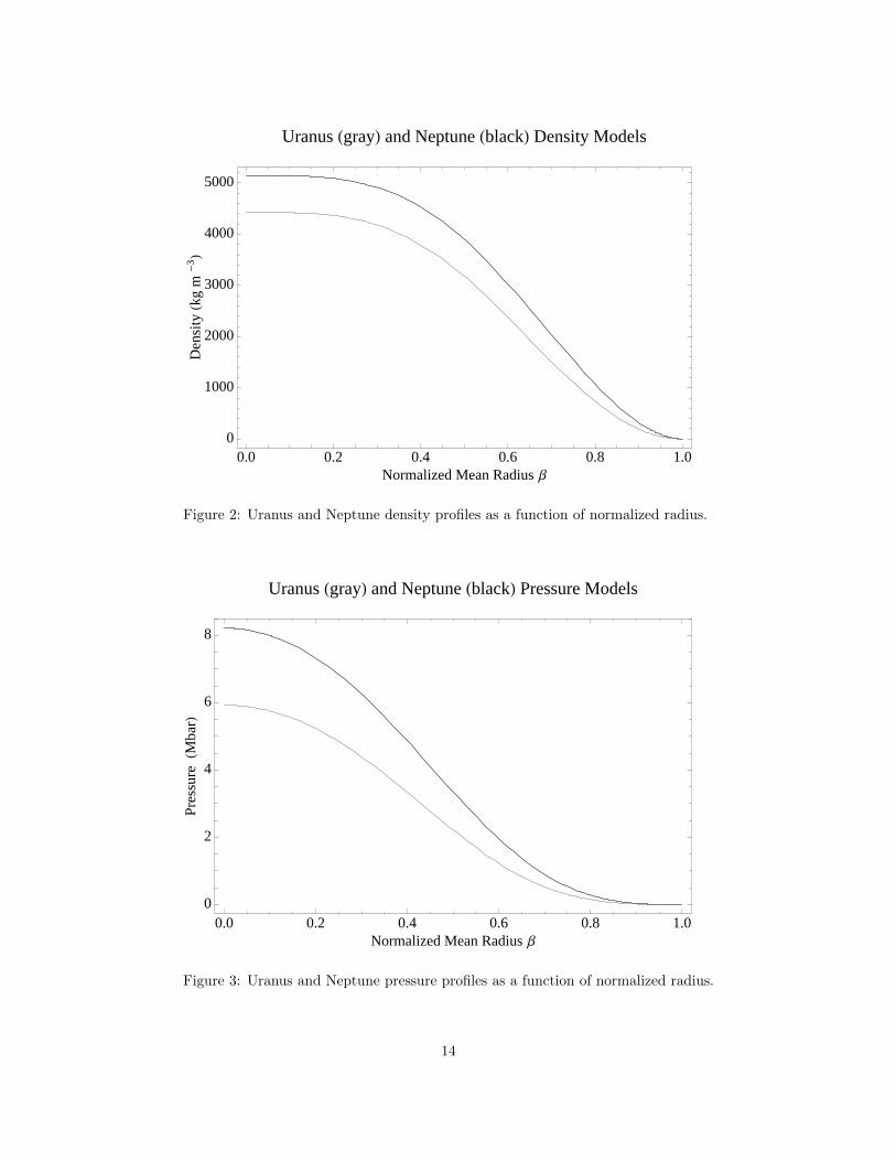
Figure 2 presents the radial density profiles of Uranus (gray curve) and Neptune (black curve) found from

the interior models. Neptune’s density is found to be higher than Uranus’ in agreement with previous models.

It has been suggested that the higher density results from Neptune’s greater compression (higher mass) and

not from compositional differences (Hubbard et al. 1991; Marely et al. 1995, Podolak et al. 1995). Figure

3 shows the radial pressure profiles of Uranus and Neptune. The gray and black lines correspond to Uranus

and Neptune, respectively. Figure 3 combines the results in the previous figures to produce pressure-density

relations for Uranus and Neptune. The pressure-density profiles can be referred to as empirical EOSs for the

planets; the EOSs of the two planets are similar.

[Figure 3]

Below we use the derived pressure-density profiles to investigate the possible compositional structures of the

planets using physical equations of state for hydrogen, helium, rock (SiO2), and ice (H2O).

3 Composition and Structure

In this section we use the empirical ρ-p relations for compositional interpretation. Although Uranus and

Neptune are known as ’icy planets’, there is no direct evidence that they actually consist of a significant

amount of ices. We consider two different possible compositions. The first is a mixture of rock (represented

by SiO2) with a hydrogen and helium mix (in the solar ratio), and the second a mix of ice (H2O) with solar

hydrogen and helium. In reality, the rocks and ices are likely to coexist, however, considering both materials

will introduce still another free parameter in the model. For simplicity, and in order to minimize the number

of free parameters, we separate the two cases. For hydrogen and helium we use SCVH EOS (Saumon et al.,

1995). This EOS is based on free energy minimization, and is currently the one most commonly used for

astrophysical applications.

To describe the heavy elements in the interior model we use the EOS of silicon dioxide (SiO2) and of water

(H2O) that are based on tables kindly supplied by D. Young (Young and Corey 1995; More et al., 1988).

The density of the mixture is calculated by the “additive-volume rule” (Saumon at al., 1995),

1

ρ(P, T )=

X

ρH+

Y

ρHe+

Z

ρZ, (3)

where X is the hydrogen mass fraction, Y is the mass fraction of helium defined by Y ≡ 1 −X − Z, Z is

the mass fraction of the high-Z material, and ρi is the density of each component.

The entropy of the mixture is given by,

S(P, T ) = XSH(P, T ) + Y SHe(P, T ) + ZSZ(P, T ) + Smix(P, T ), (4)

5

where SH , SHe and SZ are the entropy of hydrogen, helium, and silicon dioxide, respectively. Smix is the

entropy of the mixture given by Smix = kB(NlnN −∑NilnNi), where N is the total number of particles

(including free electrons), Ni is the total number of particles of component i (number of nuclei and electrons),

and kB is Boltzmann’s constant. When computing a mixture in our model, we first use the EOS of each

individual material and then combine it with the others by using the additive-volume rule to compute the

total density and the energy by using the entropy as given by eq. 4.

3.1 Uranus

At a pressure of 1 bar our Uranus model has a density of 3.5×10−4 g cm−3. An ideal gas under these

conditions and at a temperature of T = 75 K will have a mean molecular weight of 2.2, which is very close

to the value for a solar mix of hydrogen and helium. We take this as our starting point. The temperature

must increase toward the center of the planet. For an adiabat through a Debye solid, the temperature and

density are related by

T = Cργ (5)

where C and γ are constants that depend (among other things) on composition. Though we have noted

above that the temperature gradient in Uranus need not be adiabatic we nevertheless use eq. 5 as a simple

and a representative formula for the internal thermal state.

The central pressure in the Uranus model is 5.93 Mbar, so that unless the temperature at the center is

significantly higher than 104 K, the density will be very close to 7 g cm−3. The model density is 4.42 g

cm−3, so the center of the planet cannot be pure SiO2, but must contain an admixture of lighter material.

The central density and pressure can be fit, at T = 104 K with a mixture of H, He and SiO2 where H and

He are in solar proportions (X = 0.112, Y = 0.038) and SiO2 has a mass fraction Z = 0.85. A more careful

calculation using eq. 5 to estimate the temperature also gives Z = 0.85. Of course it is more likely that the

composition of both cores is actually a mixture of rock and ice, but, as Podolak et al. (1991, Table 1) have

shown, a mixture of H, He, and rock, will mimic the pressure-density behavior of ice.

Since the pressure-density relation near the surface is well-matched by a solar-composition mixture of H

and He, we consider a compositional model where the mass fraction Z of SiO2 increases from zero near the

surface to its value at the center. Lacking any guidance as to the functional form of this increase, we assume

a linear increase in Z with log ρ from Z = 0 at log ρ = −0.455 to Z = 0.85 at log ρ = 3.646. To estimate

the temperature we use eq. 5 with γ= 0.5, which is the asymptotic value of γ for high pressure. At lower

pressures γ will be higher. As a result, our procedure underestimates the temperature in the lower pressure

regions of the planet, but it gives us a feeling of whether the proposed compositional model makes any sense.

We call this model case I.

We repeat the above calculations with H2O representing the high-Z material. Figure 5 shows the com-

parison between a 6th order polynomial that fits all the gravitational data (black solid curve) and the

compositional model described above with rock (black dashed curve) and ice (gray dashed curve). As can

be seen from the figure, the behavior of the calculated EOS curves are very close to each other although the

curve representing a mixture of hydrogen and helium with ices is slightly closer to curve of the empirical

ρ-p relation. Considering the crudeness of the approximations involved, the fits are quite good. It is not

surprising that the density at intermediate pressures is too high. This is most likely due to our underestimate

of the temperature in that region. Certainly the details of the temperature gradient and the compositional

gradient can be adjusted to provide a better fit. In any case, it seems quite clear that a Uranus model with

6

an adiabat-like temperature gradient and a continuous increase in Z toward the center can be made to fit

the observed parameters of the planet.

We next investigate the possibility of a different compositional configuration. We consider a three-layer

model, where the outermost layer has Z constant and equal to its value at the surface; the innermost layer

has Z constant and equal to its value at the center, and the middle layer has Z varying linearly with log ρ

between the surface value and the central value. The beginning and end of this central ”transition region” is

determined by getting a good fit to the empirically determined EOS. We call this model case II. This model

gives a surprisingly good fit to the empirical curve and is presented as black (rock) and gray (ice) dots in

Figure 5. Remarkably the transition region begins at a temperature of around 1500 K, which is just the

region where silicates begin to vaporize. The overall composition of Uranus is essentially the same for case

I and case II (see table 3).

3.2 Neptune

The best fit polynomial gives a 1-bar density for Neptune of 4.38×10−4 g cm−3. For an ideal gas at this

pressure and at T = 75 K, the mean molecular weight is 2.7. This is significantly higher than the 2.3

appropriate for a solar mix of H and He. Although the vapor pressure of SiO2 at this temperature is

extremely low, for the purposes of this comparison we assume that SiO2 vapor supplies the additional

molecular weight. Its mass fraction at the 1-bar level must then be Z = 0.0073. Again we assume that the

temperature is given by eq. 5, so that the central temperature is 8.1×103 K. At this temperature, and at a

central pressure of 8.22 Mbar as determined from the polynomial fit, the central density of 5.15 g cm−3 is

fit by Z = 0.82. This is very similar to the value determined for Uranus.

If we assume that Z increases linearly in log ρ as before (case I), we find that the pressure-density relation

is given by the dashed curve in fig. 6. This is quite close to the pressure-density relation determined by a

polynomial fit to Neptune’s observed parameters (black solid curve in fig. 6). A case II model of Neptune

gives similar results. Here the transition region begins at a somewhat lower temperature, ∼ 1400 K.

For both Uranus and Neptune the polynomial fit and the proposed compositional model differ in the same

way. For case I both Uranus and Neptune have too high a density at intermediate pressures, indicating that

the assumed temperature there is too low or Z is too high. Nearer to the center the density is somewhat too

low for both planets. In this region the temperature dependence of the pressure is small, so it is more likely

that a somewhat faster than linear increase in Z is indicated. In any case, essentially the same compositional

model works for both Uranus and Neptune. For case II both planets show the same overall structure. The

transition region for both planets begins at around 1500 K. The big difference between the two planets is

that Neptune requires a non-solar envelope while Uranus is best matched with a solar composition envelope.

A similar result was found by Podolak et al. (1995), but it was not clear how much of this difference was due

to the detailed assumptions of the internal structure and temperature distribution. We find a qualitatively

similar result simply from a polynomial fit to the observed gravity field. Finally, we note that both H2O and

SiO2 match the polynomial fit equally well.

The model fits can be used to derive the relative amounts of each component (mass fractions). For case

I we find that when SiO2 is used, Uranus’s interior is found to consists of 18.1% hydrogen, 6.2% helium, and

75.7% rock. Neptune’s composition is found to be 18.1.% hydrogen, 6.2% helium, and 75.8% rock. When

H2O is used, Uranus’ interior is found to consist of 8.48% and 2.88% of hydrogen and helium, respectively,

and 88.6% of ice. Neptune’s composition is found to be 8.0% hydrogen, 2.7% helium, and 89.3% ices. For

7

case II we find that Uranus consists of 16.4% hydrogen, 5.56% helium, and 78.1% rock. When H2O is used,

Uranus’ interior is found to consist of 6.41% and 2.18% of hydrogen and helium, respectively, and 91.4% of

ice. Neptune’s composition is found to be 17.5.% hydrogen, 6.94% helium, and 76.6% rock. When water is

used to represent the high-Z material, Neptune’s interior is found to consist of 7.19% and 2.44% of hydrogen

and helium, respectively, and 90.4% of ice. The results are summarized in table 3. It is clear that the

compositions of the planets are similar, and as expected, the high-Z mass fraction increases when a lighter

material (H2O) is used to represent the heavy elements.

Table 3

The compositions listed above are not meant to represent the actual compositions of Uranus and Neptune

but are only the compositions derived under our simple interpretation of the polynomial fit. In addition,

as we mentioned earlier, the planets are likely to consist of a mixture of both ice and rock. Clearly more

detailed theoretical models are necessary.

4 Discussion and Conclusions

We present phenomenological pressure-density profiles for Uranus and Neptune. These models show that

the gravitational fields (J2, J4) of both Uranus and Neptune could be reproduced with continuous radial

density distributions (no density jumps). In addition, the internal structures of the planets are found to be

similar. We use equations of state for hydrogen and helium, and high-Z material (SiO2 or H2O) to interpret

the empirical EOS in terms of compositional structure. Our analysis suggests that Uranus and Neptune

could have similar composition and structure. We find that the empirical EOS for both planets can be fit

by assuming a gradual increase of the heavier material toward the center, with hydrogen and helium being

kept at solar ratio. For case I, when SiO2 (rock) is used to represent the high-Z material in the interior,

the masses of heavy elements are found to be 10.9 and 12.9 M⊕ for Uranus and Neptune, respectively. The

innermost regions of both Uranus and Neptune cannot be fit to the empirical EOS by pure rock, but by ∼82% rock by mass for both planets with the rest being a mixture of hydrogen and helium in solar ratio.

When H2O is used to represent high-Z material the masses of heavy elements are found to be higher due

to the lower density of water compared with rock. The heavy element masses are found to be ∼ 12.8 and

15.2 M⊕ for Uranus and Neptune, respectively. Even when water is used, the planetary centers are found to

contain gases in addition to the high-Z material, though the Z mass fraction at the centers are found to be

above 90% for both planets. Again, the results imply that the interiors of Uranus and Neptune could have

concentrations of high-Z material increasing gradually toward their centers. A similar situation might occur

in the gas giant planets, Jupiter and Saturn, and we suggest that a gradual increase of the heavier elements

should be considered when modeling giant planet interiors. For case II the SiO2 contents for Uranus and

Neptune are 11.3 and 13.1 M⊕, respectively, while for H2O the values are 13.2 and 15.4 M⊕.

The interior structures of Uranus and Neptune are poorly understood, and their interiors may be quite

different from the ’traditional 3-layer’ models. A 3-layer model is often used to model interior structures of

Neptune/Uranus-like extrasolar planets, while the true interiors of Uranus and Neptune may differ signifi-

cantly from such a structure. We therefore suggest that more flexible interior structures should be considered

when modeling extrasolar planet interiors.

8

Acknowledgments

R. H. and J. D. A acknowledge support from NASA through the Southwest Research Institute. M. P.

acknowledges support from ISF 388/07. G. S. acknowledges support from the NASA PGG and PA programs.

5 References

Anderson, J. D. and Schubert, G. ”Saturns Gravitational Field, Internal Rotation, and Interior Structure.”

Science 317: (2007) 1384—1387.

Guillot, T., 1999. A comparison of the interiors of Jupiter and Saturn. Planetary and Space Science, 47, p.

1183–1200.

Guillot, T. and Gautier, D., 2007, Giant Planets, Treatise of Geophysics, vol. 10, Planets and Moons, Schu-

bert G., Spohn T. (Ed.) (2007) 439-464. eprint arXiv:0912.2019.

Helled, R., G. Schubert, and J. D. Anderson. Empirical models of pressure and density in Saturn’s inte-

rior: Implications for the helium concentration, its depth dependence, and Saturn’s precession rate, Icarus,

2009(a), 199, 368–377.

Helled, R., Schubert, G. and Anderson, J. D. Jupiter and Saturn Rotation Periods. Planetary and Space

Science, 2009(b), 57, 1467–1473.

Helled, R., J. D. Anderson, and G. Schubert. Uranus and Neptune: Shape and Rotation”. Icarus, 2010, in

press.

Hubbard, W. B., 1968. Thermal structure of Jupiter. Astrophys. J., 152:745–754.

Hubbard, W. B., Nicholson, P. D., Lellouch, E., Sicardy, B., Brahic, A., Vilas, F., Bouchet, P., McLaren, R.

A., Millis, R. L., Wasserman, L. H., Elais, J. H., Matthews, K., McGill, J. D., Perrier, C., 1987. ”Oblateness,

radius, and mean stratospheric temperature of Neptune from the 1985 August 20 occultation”, Icarus, 72,

635–646.

Hubbard, W. B., Nellis, W. J., Mitchell, A. C., Holmes, N. C., McCandless, P. C., and Limaye, S. S. (1991).

Interior structure of Neptune - Comparison with Uranus. Science, 253, 648–651.

Lindal, G. F. The atmosphere of Neptune - an analysis of radio occultation data acquired with Voyager 2.

Astron. Jour. 103: (1992) 967982.

Lindal, G. F., Sweetnam, D. N., and Eshleman, V. R. 1985, The atmosphere of Saturn - an analysis of the

Voyager radio occultation measurements. AJ, 90, 1136–1146.

Lindal, G. F., J. R. Lyons, D. N. Sweetnam, V. R. Eshleman, and D. P. Hinson. The atmosphere of Uranus

- Results of radio occultation measurements with Voyager 2. Jour. Geophys. Res. 92: (1987) 14,98715,001.

Lodders, Katharina, and Bruce Fegley, Jr. The Planetary Scientists Companion. New York Oxford: Oxford

University Press, 1998.

Lyon, S. P. and Johnson, J. D., 1992. SESAME: The Los Alamos National Laboratory equation of state

database. website, http://t1web.lanl.gov/doc/SESAME-3Ddatabase1992.html.

Marley, M. S., Gmez, P., and Podolak, M., 1995. Monte Carlo interior models for Uranus and Neptune.

Journal of Geophysical Research, 100, 23349–23354.

More, R.M, Warren, D.A., Young, D.A & Zimmerman, G.B. ,1988. A new quotidian equation of state

(QEOS) for hot dense matter. Physics of Fluids, 31,10, 3059–3078.

Ness, N. F., Acuna, M. H., Behannon, K. W., Burlaga, L. F., Connerney, J. E. P., Lepping, R. P., 1986.

Magnetic fields at Uranus. Science, 233, pp. 8–89.

9

Ness, N. F., Acuna, M. H., Burlaga, L. F., Connerney, J. E. P.; Lepping, R. P., 1989. Magnetic fields at

Neptune. Science, 246, pp. 1473–1478.

Pearl, J. C., Conrath, B. J., Hanel, R. A., Pirraglia, J. A., and Coustenis, A., 1990. The albedo, effective

temperature, and energy balance of uranus, as determined from voyager iris data. Icarus, 84:12–28.

Podolak, M. and Hubbard, W. B., 1998. Ices in the giant planets. In . M. F. B. Schmitt, C. de Bergh, ed.,

Solar System Ices, pp. 735–748.

Podolak, M., Hubbard, W.B. and Stevenson, D.J. Models of Uranus’ interior and magnetic field. Uranus,

ed. J. Bergstrahl and M. Matthews, Un. Arizona Press, pp.29-61, 1991.

Podolak, M., Weizman, A., and Marley, M., 1995. Comparative models of Uranus and Neptune. Planetary

and Space Science, 43, 1517–1522.

Podolak, M., Podolak, J. I., and Marley, M. S., 2000. Further investigations of random models of Uranus

and Neptune. Planet. & Sp. Sci., 48:143–151.

Smith, B. A., L. A. Soderblom, D. Banfield, C. Barnet, R. F. Beebe, A. T. Bazilevskii, K. Bollinger, J. M.

Boyce, G. A. Briggs, and A. Brahic. Voyager 2 at Neptune - Imaging science results. Science 246: (1989)

14221449.

Smith, B. A., L. A. Soderblom, R. Beebe, D. Bliss, R. H. Brown, S. A. Collins, J. M. Boyce, G. A. Briggs,

A. Brahic, J. N. Cuzzi, and D. Morrison. Voyager 2 in the Uranian system - Imaging science results. Science

233: (1986) 4364.

Stacey, Frank D. Physics of the Earth. Brisbane: Brookfield Press, 1992.

Stanley, S. and Bloxham, J., 2004. Convective-region geometry as the cause of Uranus’ and Neptune’s un-

usual magnetic fields. Nature, 428, pp. 151–153.

Stanley, S. and Bloxham, J., 2006. Numerical dynamo models of Uranus’ and Neptune’s magnetic fields.

Icarus, 84, p. 556–572.

Saumon, D., Chabrier, G., & Van Horn, H.M. 1995, An equation of state for low-mass stars and giant plan-

ets. The Astrophysical Journal, 99, 713–741.

Saumon,D. & Guillot,T., 2004. Shock Compression of Deuterium and the Interiors of Jupiter and Saturn.

The Astrophysical Journal, 609, 1170–1180.

Smith, B. A., L. A. Soderblom, D. Banfield, C. Barnet, R. F. Beebe, A. T. Bazilevskii, K. Bollinger, J. M.

Boyce, G. A. Briggs, and A. Brahic., 1989. Voyager 2 at Neptune - Imaging science results. Science 246,

1422–1449.

Tyler, G. L., Sweetnam, D. N., Anderson, J. D., Borutzki, S. E., Campbell, J. K., Kursinski, E. R., Levy,

G. S., Lindal, G. F., Lyons, J. R., Wood, G. E., 1989. Voyager radio science observations of Neptune and

Triton. Science, 246, 1466–1473.

Young, D.A. & Corey, E.M., 1995. A new global equation of state model for hot, dense matter. J.Appl.Phys.,

78:3748–3755.

Zharkov, V. N. and Trubitsyn, V. P. , 1974. Determination of the equation of state of the molecular envelopes

of Jupiter and Saturn from their gravitational moments. Icarus, 21, 152–156.

Zharkov, V. N., and V.P. Trubitsyn. Physics of Planetary Interiors. Tucson: Pachart, 1978.

10

Parameter Uranus Neptune

P (rotation period) 17.24h 16.11h

GM (km3 s−2) 5,793,964 ± 6 6,835,100. ± 10

Rref (km) 26,200 25,225

J2 (×106) 3341.29 ± 0.72 3408.43 ± 4.50

J4 (×106) -30.44 ± 1.02 -33.40 ± 2.90

a (km) 25,559 ± 4 24,764 ± 15

J̄2 (×106) 3510.99 ± 0.72 3536.51 ± 4.50

J̄4 (×106) -33.61 ± 1.02 -35.95± 2.90

q 0.0295349 0.0260784

ρ0 (kg m−3) 1266.46 1630.53

p0 (Mbar) 2.89025 4.51959

Table 1: Physical data, taken from JPL database: http://ssd.jpl.nasa.gov, Jacobson (2003), Jacobson et al. (2006).

Rref is an arbitrary reference equatorial radius associated with the reported values of the measured gravitational

harmonics J2 and J4. a is the equatorial radius at the 1 bar pressure level. J̄2 and J̄4 are the values taken by

the gravitational coefficients when referenced to a instead of Rref. q, ρ0 and p0 are the smallness parameter, the

characteristic density, and the pressure, respectively, as defined in the text.

Parameter Uranus Neptune

J2 (×106) 3341.31 3408.65

J4 (×106) -30.66 -30.97

J6 (×106) 0.4437 0.4329

J̄2 (×106) 3511.01 3536.74

J̄4 (×106) -33.85 -33.34

J̄6 (×106) 0.5148 0.4836

Table 2: Interior model results. J2n are the gravitational moments corresponding to the reference radii,

Rref, while ¯J2n correspond to the gravitational coefficients normalized by a the equatorial radius at 1 bar.

The values should be compared with the measured values given in Table 1.

11

SiO2 H2O

Case I: Uranus X = 0.181; Y = 0.0616; Z = 0.757 X = 0.0848; Y = 0.0288; Z = 0.886

Case I: Neptune X = 0.181; Y = 0.0615; Z = 0.758 X = 0.0795; Y = 0.027; Z = 0.893

Case II: Uranus X = 0.164; Y = 0.0556; Z = 0.781 X = 0.0641; Y = 0.0218; Z = 0.914

Case II: Neptune X = 0.175; Y = 0.0694; Z = 0.766 X = 0.0719; Y = 0.0244; Z = 0.904

Table 3: Derived planetary compositions (given in mass fractions) for Uranus and Neptune. The two

different columns correspond to different materials representing the heavy elements (SiO2 and H2O). The

hydrogen to helium ratio (X/Y) is set to the protosolar value. Case I corresponds to a model assuming a

linear increase in Z from the surface to the planet’s center. Case II corresponds to an interior structure

consists of three-layers with a constant composition in the central region (core) and the atmosphere with a

middle ’transition region’ with Z increasing toward the center (see text for details). The sum of the mass

fractions do not exactly total to one because of numerical roundoff.

12

core

J0

J2

J4

J6

0.0 0.2 0.4 0.6 0.8 1.00

1

2

3

4

Normalized Mean Radius Β

Con

trib

utio

nfu

nctio

ns

Jupiter

core

J0

J2

J4

J6

0.0 0.2 0.4 0.6 0.8 1.00

1

2

3

4

Normalized Mean Radius Β

Con

trib

utio

nfu

nctio

ns

Neptune

Figure 1: Normalized integrands of the gravitational moments (contribution functions) of Jupiter (top) and

Neptune (bottom). The values are normalized to make the area under each curve equal unity. J0 is equivalent

to the planetary mass. The range of possible core sizes is indicated. Here, core designates a region of heavy

elements below the H/He envelope. It is clear that Neptune’s (Uranus’) interior is better sampled by the

gravitatioal harmonics compared to Jupiter (Saturn).

13

0.0 0.2 0.4 0.6 0.8 1.00

1000

2000

3000

4000

5000

Normalized Mean Radius Β

Den

sity

Hkg

m-

3 L

Uranus HgrayL and Neptune HblackL Density Models

Figure 2: Uranus and Neptune density profiles as a function of normalized radius.

0.0 0.2 0.4 0.6 0.8 1.00

2

4

6

8

Normalized Mean Radius Β

Pres

sure

HMba

rL

Uranus HgrayL and Neptune HblackL Pressure Models

Figure 3: Uranus and Neptune pressure profiles as a function of normalized radius.

14

0 1 2 3-6

-5

-4

-3

-2

-1

0

1

Log Density Hkg m -3L

Log

Pres

sure

HMba

rL

EOS for Uranus HgrayL and Neptune HblackL

Figure 4: Uranus and Neptune empirical ρ(p) relations.

-6 -5 -4 -3 -2 -1 0

0

1

2

3

LogP HMbarL

Log

ΡHk

gm

-3 L

Uranus

Figure 5: Pressure density relation for a Uranus model. The black solid curve is the polynomial that fits the

gravitational data. The black and gray dashed curves are the compositional models described in the text

taking the high-Z material to be SiO2 and H2O, respectively (Case I). The black and gray points are for

Case II and correspond to rock and ice, respectively.

15

-6 -5 -4 -3 -2 -1 0 1

0

1

2

3

LogP HMbarL

Log

ΡHk

gm

-3 L

Neptune

Figure 6: Pressure density relation for a Neptune model. The black solid curve is the polynomial that fits

the gravitational data. The black and gray dashed curves are the compositional models described in the

text taking the high-Z material to be SiO2 and H2O, respectively (Case I). The black and gray points are

for Case II and correspond to rock and ice, respectively.

16