-

unibz junior researcher

Dario Prando

Energy Conversion and Distribution to the End User

Use of Biomass in SouthTyrol

Use of Biomass in SouthTyrolDario Prando

unibz junior researcher

Energy Conversion and Distribution to the End User

Cover design: doc.bz / bu,press

Printer: Druckstudio Leo, Frangart/o

© 2016 by Bozen-Bolzano University Press

www.unibz.it/universitypress

This work—excluding the cover and the quotations—is licensed under the Creative

Commons Attribution-ShareAlike 4.0 International License.

ISBN 978-88-6046-087-5

E-ISBN 978-886046-124-7

Contents

The unibz junior researcher series .......................................................................... VII

Acknowledgements ................................................................................................. XI

Preface ................................................................................................................... IX

1. Introduction and literature review ................................................................... 1

1.1 Biomass for CHP generation ......................................................................... 2

1.2 Biomass for district heating ......................................................................... 11

2. CHP plant based on biomass boiler and ORC generator .............................. 21

2.1 Materials and methods ................................................................................ 24

2.2 Results and discussion ................................................................................ 35

2.3 Main findings .............................................................................................. 42

3. CHP plant based on gasifier and ICE ........................................................... 45

3.1 Materials and methods ................................................................................ 47

3.2 Results and discussion ................................................................................ 51

3.3 Main findings .............................................................................................. 54

4. Critical issues on biomass-to-energy systems .............................................. 55

4.1 Experimental setup ..................................................................................... 59

4.2 Results and discussion ................................................................................ 63

4.3 Main findings .............................................................................................. 72

5. Integrated assessment of gasification systems for residential application ...... 73

5.1 Methodology ............................................................................................... 75

5.2 Results and discussion ................................................................................ 85

5.3 Main findings .............................................................................................. 92

6. Building refurbishment and DH systems ....................................................... 94

6.1 Materials and methods ................................................................................ 97

6.2 Results and discussion .............................................................................. 108

6.3 Main findings ............................................................................................ 121

7. Conclusions .............................................................................................. 123

Nomenclature ....................................................................................................... 129

References ........................................................................................................... 133

The author ............................................................................................................ 153

VII

The unibz junior researcher series

Especially at a time when universities are increasingly expected to produce

tangible results, it is clear that one of their main tasks is to promote the work

of their young scientists. The decision by the Free University of Bozen-Bol-

zano to publish the new series unibz junior researcher, enabling PhD students

to present their research to a wider readership, is designed not so much to

promote the work of individual scholars but rather to foster a common

university culture. The idea is to publish studies which are exemplary, not

just within the standards of the individual discipline, but also because of the

wider significance of the issues they deal with and the way they are dealt

with.

Due to the ever-increasing pressure in the academic world to publish papers

in internationally-renowned journals, there is a danger that a lot of research

reaches out to only a narrow field of specialists. But we maintain that it is

precisely the role of the university to ensure that knowledge is transmitted to

a wider audience, that discussion between different areas of research is

stimulated and that a dialogue with a wider readership beyond the univer-

sity is established. This promotes a public sphere that is better informed and

more competent in debating. The studies which are published in the unibz

junior researcher series will serve future PhD students as reference points for

participation in such a culture of research. Engaging in research in isolation

from the general public simply ignores the requirements of our times:

Universities need to open up and academics need to learn to transmit their

knowledge at various levels—all the more so considering the increasing

complexity of research topics and the higher demands of research methods.

This is the only way to justify public investment in universities, only in this

way can universities fulfil their public mandate and contribute to a compe-

tent dialogue over impending societal issues.

VIII

The first issues of this series convincingly fulfil these criteria. They present

PhD research projects judged as excellent by the examining commissions.

The Free University of Bozen-Bolzano’s excellent research environment has

contributed greatly to these results: The authors were able to approach their

research topics in a measured way, under the close supervision of members

of the respective PhD advisory commission, who were able to offer a range

of perspectives on the relevant research methodology. Furthermore, the uni-

versity's generous bursary scheme gives PhD students the opportunity to

spend periods of study and research abroad, and to thereby gain experience

of how other universities conduct research on related topics. They could also

present their research methodology and preliminary findings at interna-

tional congresses – a valuable experience in improving communicative com-

petences. Finally, the regional setting of our university gave them access to a

rich variety of empirical data which shows that South Tyrol, while being an

alpine region, is by no means represents “periphery”. Instead, the research

projects demonstrate that regional study objects can have international

relevance because the condensed dimensions allow processes to be brought

into focus more readily and changes to be monitored more precisely. The

region of South Tyrol is indeed affected by global change, as witnessed for

instance in the environmental field, where its sensitive alpine landscape is

particularly susceptible to harmful developments. So it is possible to see

South Tyrol as a sort of laboratory where we can register warning signs

earlier and experiment with appropriate counter measures. A greater density

of transformation processes can equally be seen in the social field. As a

traditional border area, South Tyrol has always been at the crossroads of

different cultures. Its historical experience with multilingualism, with differ-

rent political and legal frameworks and with the cultural interaction of very

different reference points for identity, makes for a background against which

some of today’s major social challenges such as migration or the globalised

economy, can be analysed and interpreted.

These chances for new socially-relevant scientific insights find expression in

the PhD studies selected for this series. The university authorities hope that

these publications will allow the wider public to gain insights into the qua-

IX

lity of the work of these young researchers, and to recognize that the fruits of

the financial investment in this university have direct beneficial effects on

the local society. I congratulate the authors chosen for this series and wish

them every success in their scientific career hoping they will remain intel-

lectually and emotionally linked to their university and to South Tyrol.

Walter Lorenz

Rector – Free University of Bozen-Bolzano

XI

Acknowledgements

This research work was financially supported by the Autonomous Province

of Bolzano in the main framework of the project “Sustainable use of biomass

in South Tyrol: from production to technology”. I thank Prof. Zerbe, who

coordinated the project.

A special thanks goes to my supervisors Prof. Gasparella, Prof. Baratieri and

Prof. Dasappa for teaching me the secrets of research and making me feel at

home, both in Italy and in India. I am also grateful to Prof. Righetto, Prof.

Zaffani and Prof. Longo, who lit my way from the middle school up to

university.

I would like to thank all the friends who accompany me on my journey, in

particular, the biomass guys, the buildings guys, the PhD guys and the

CGPL guys.

Last but not least, my gratitude goes to my family, and to my wife Stefy in

particular, for her constant support and for her enormous commitment for

our new family.

XIII

Preface

This book is the result of a PhD research, based on both modelling and expe-

rimental studies in the area of renewable energy. The research was con-

ducted in Italy at the Free University of Bolzano and complemented with re-

search at the Indian Institute of Science in Bangalore (India). This collabora-

tion was established through the SAHYOG project, which aims at strength-

ening the network between Europe and India. In addition, other cooperation

initiatives with national and international scientific partners have been es-

tablished, such as with the University of Florence, the University of Trento,

the University of Innsbruck, and with companies such as Bioenergy 2020+,

Bioenergie Renon, EcoResearch, Re-Cord, SIBE and Tis Innovation Park. This

research was financially supported by the Autonomous Province of Bo-

zen-Bolzano within the main framework of the project “Sustainable use of

biomass in South Tyrol: from production to technology” coordinated by

Stefan Zerbe.

Renewable energy and energy efficiency is at the top of the political agenda

both in Europe and worldwide. The European Union has issued various

directives for the promotion of the use of renewable energy and the energy

efficiency of both buildings and energy conversion systems. All these

measures are considered viable options to reduce both greenhouse gas emis-

sions as well as the dependence on imported fossil fuels. Moreover, when

referring to the efficiency of a system, it is imperative not to refer only to the

nominal efficiency of each single component but to the global efficiency of

the entire system. This aspect is a key point to develop efficient systems, and

it requires tools and skills to identify the optimal solution for a specific

application.

With this volume the author aims at providing an insight into the

above-mentioned issues by presenting an integrated assessment of the per-

formance of energy conversion systems based on lignocellulosic biomass. On

XIV

the one hand, it focuses on the conversion of biomass into energy, on the

other hand, on the distribution and matching of the generated heat to the

demand, i.e. the final uses, considering the respective efficiencies. These two

elements are complementary and both their efficiencies contribute to the

overall performance of the whole system.

One of the challenges of this topic involves the improvement of bio-

mass-to-energy systems identifying possible upgrading measures and—in

particular for the gasification-based plants—the enhancement of the opera-

tional reliability. Nonetheless, the subsidy mechanism for the promotion of

renewable energy should be revised since it strongly favours the profitability

of electricity production compared to heat production. In this perspective,

the first part of the work deals with the detailed monitoring of two commer-

cially available plants—one based on combustion and one on gasification—

in order to define the current energy performance achievable in practical ap-

plications. The experimentation has been supplemented with the modelling

of the main components in order to identify potential improvements. Since

the operational reliability of gasification systems is threatened by the pres-

ence of tar compounds in the producer gas, a base study on tar characterisa-

tion was carried out during the research at the Indian Institute of Science in

Bangalore. In fact, tar is considered the main barrier for the development of

gasification technology. However, the research has shown that technology

packages do exist to meet the demand.

Another challenge that needs to be met is the prediction of the impact of

building refurbishment on the energy performance of the systems. Nowa-

days, both subsidies and minimum requirements are set by the governments

to promote improvements in building energy performance. This rapidly

changes the building scenario and it also requires a constant update of the

energy systems to be efficient in real operation. Furthermore, when consid-

ering the installation of small scale combined heat and power (CHP) systems

based on biomass, there is a limit on the minimum scale available in the

market. In this perspective, the CHP installation is rarely suitable for a single

building and the use of district heating (DH) networks is required to justify

this application. Nonetheless, the DH network should not compromise the

heat distribution efficiency that would affect the global efficiency of the

XV

system. In this framework, the second part of this work deals with the

energy and economic assessment of the distribution and use of the heat

generated by a plant. A numerical model, developed for the purpose,

enables the simulation of both centralised users (building, flat) and distrib-

uted users (district heating). The impact on the whole system of both the

refurbishment of the buildings and the potential improvement of the DH

network has been investigated exploiting the prediction capabilities of the

developed model.

The main results of this research highlight that, in most of the CHP plants, a

considerable share of the heat is discharged into the environment because

the subsidisation mechanism makes heat generation less profitable than

electricity. Moreover, gasification systems have shown higher electrical effi-

ciency than Organic Rankine Cycle (ORC) systems, however the latter could

increase the performance if operated with a heat sink at low temperature.

Therefore, the conversion of the current district heating networks to low

temperature systems could considerably improve the heat distribution

efficiency and, consequently, the efficiency of the whole system. The future

refurbishment of buildings will be a great challenge for the DH networks,

which will need to consider improvement measures, such as low

temperature distribution and CHP system installation, to be competitive

against alternative solutions.

This study is undoubtedly a tangible contribution to spread the know-how

acquired from an extensive investigation into the sustainable use of ligno-

cellulosic biomass and it paves the way for the implementation of efficient

energy systems from a global perspective.

A. Gasparella – Free University of Bozen-Bolzano, Italy

M. Baratieri – Free University of Bozen-Bolzano, Italy

S. Dasappa – Indian Institute of Science, Bangalore, India

1

1. Introduction and literature review

Biomass, wood in particular, is the oldest source of energy used by mankind.

It still represents roughly 9 % of the world’s primary energy consumption

and 65 % of the world’s renewable primary energy consumption (Lauri et al.

2014). Nowadays, this renewable energy resource is considered as an option

to reduce both greenhouse gas emissions and the dependence on imported

fossil fuels (The European Parliament and the Council of the European

Union 2009). The process involving growth and combustion of biomass is

carbon neutral because CO2, emitted during combustion, is sequestered by

process of photosynthesis from the atmosphere during the growth of the

plant. Furthermore, the emitted CO2 is twenty times less active as green-

house gas than methane which would be produced from the natural decom-

position of biomass (Demirbas 2001). Nevertheless, biomass usually needs

pre-processing to become a suitable fuel and has to be transported to the en-

ergy generation plant; all these steps negatively impact on the greenhouse

gas emissions.

Cogeneration is defined as the combined production of heat and power and

allows a primary energy saving compared to the separate production of the

two energy streams. With regard to the limited availability of renewable

resources, among them especially biomass resources, efficiency in terms of

consumption and utilization becomes vital. Heat is the energy stream with

lower quality and it is generated in most of the conversion processes. Ther-

modynamically, the lower the exit temperature of the flue gases from the

process plant, the higher the efficiency of the polygeneration system. For this

reason, a polygeneration system is suitable to be coupled to a DH system

which enables exploiting heat at quite low temperature (i.e. < 100 °C). Fur-

thermore, future implementation of the fourth generation DH (i.e. re-

turn/supply temperatures at 30/70 °C) will allow exploiting heat share that

until now has usually been discharged into the environment .

The first part of this chapter deals with the main technologies for cogenera-

tion based on biomass. CHP generation technologies are then compared;

combustion-based systems (i.e. steam turbine, organic Rankine cycle and

Stirling engine) and gasification-based systems (i.e. internal combustion

2

engine and biomass integrated gasification combined cycle). Capacity

(power level), efficiency, operation flexibility and field experience at the cur-

rent state of the art have been reported for each technology.

The second part of the chapter deals with the implementation of biomass

technologies in DH systems. A brief introduction about the architecture of

DH systems has been complemented by an analysis of the potential benefits

deriving from the use of biomass. The CHP systems, presented in the previ-

ous section, are analysed focusing on their application to DH networks. The

discussion has been extended including the determination of the cost-opti-

mal size, the role of thermal energy storage and the impact of biomass trans-

portation on the energy chain. Moreover, the influence of extensive refur-

bishment on the buildings connected to DH grids is extensively analysed.

The possible solutions that allow the DH systems to be competitive in the

future are presented in accordance with the scientific literature. Finally, the

smart grid concept has been introduced and its applicability to thermal net-

works is discussed highlighting the potential benefits for the thermal sector

as well as for the entire energy system.

1.1 Biomass for CHP generation

In the past few years, there has been a great interest in renewable energy

sources. On the one hand, energy demand has been constantly growing,

strictly correlated to the increase of global population and to expansion of

developing countries’ economies (Nelson 2011). This aspect, combined with

the depletion of fossil fuels, has in the last few years caused a considerable

increase in the prices for fossil fuel energy on the global energy markets. On

the other hand, industrialized societies are currently becoming more aware

of the impacts of fossil fuel utilization on the environment and on human

health, making the search for environmentally and socially acceptable alter-

natives increasingly important (Kaltschmitt et al. 2007). If compared to other

renewable sources (e.g., wind or solar energy) biomass has the main

advantage that, if well managed, it can ensure a constant supply of energy,

its availability not being dependent on climatic conditions in the short and

medium term. This is an essential aspect in the design of an integrated

exploitation of different renewable sources.

3

Sustainable biomass feedstock should have no impact on the food chain. In

particular, lignocellulosics biomass, as woody biomass, energy crops—that

are cultivated for the purpose of energy generation—or even algae are some

examples of them. In Fig. 1.1 a rough distinction between crops, residues, by-

products and waste has been made to consider a wide spectrum of feedstock

for polygeneration. After the harvesting or collection, biomass has to be

subjected to different pre-treatments, which usually have the common pur-

pose of energy densification. The biomass chain is then characterized by

transportation and storage to the first stage of conversion, i.e. thermo-,

physical- and bio-chemical. Intermediate fuels and chemicals (solid, liquid

and gaseous) can be obtained starting from the original feedstock, which can

be valorised through combustion in boilers and, prime movers or fuel cell

stacks for heat and electricity generation both for stationary and automotive

applications.

Fig. 1.1 – Schematic representation of different biomass-to-energy pathways (rounded boxes:

energy carriers; boxes: conversion processes); Kaltschmitt et al. (2007).

4

The main technologies developed for converting biomass into thermal

energy and electricity usually include a primary conversion stage that pro-

duces hot water, steam, gaseous or liquid products and a secondary conver-

sion stage that transforms these intermediate products to heat and power. In

the present section, the thermochemical processes are considered in detail

and the different technologies are presented according to the following clas-

sification:

- combustion-based technologies producing steam or hot water, coupled to

steam engines, steam turbines, Organic Rankine Cycle (ORC) and Stirling

engines;

- gasification-based technologies producing gaseous fuels, coupled to inter-

nal combustion engines (ICEs), gas turbines (GTs), fuel cell stacks and micro-

turbines.

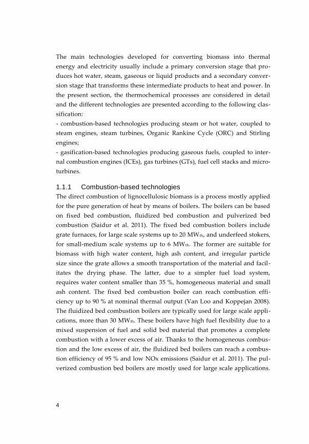
1.1.1 Combustion-based technologies

The direct combustion of lignocellulosic biomass is a process mostly applied

for the pure generation of heat by means of boilers. The boilers can be based

on fixed bed combustion, fluidized bed combustion and pulverized bed

combustion (Saidur et al. 2011). The fixed bed combustion boilers include

grate furnaces, for large scale systems up to 20 MW th, and underfeed stokers,

for small-medium scale systems up to 6 MWth. The former are suitable for

biomass with high water content, high ash content, and irregular particle

size since the grate allows a smooth transportation of the material and facil-

itates the drying phase. The latter, due to a simpler fuel load system,

requires water content smaller than 35 %, homogeneous material and small

ash content. The fixed bed combustion boiler can reach combustion effi-

ciency up to 90 % at nominal thermal output (Van Loo and Koppejan 2008).

The fluidized bed combustion boilers are typically used for large scale appli-

cations, more than 30 MWth. These boilers have high fuel flexibility due to a

mixed suspension of fuel and solid bed material that promotes a complete

combustion with a lower excess of air. Thanks to the homogeneous combus-

tion and the low excess of air, the fluidized bed boilers can reach a combus-

tion efficiency of 95 % and low NOx emissions (Saidur et al. 2011). The pul-

verized combustion bed boilers are mostly used for large scale applications.

5

The fuel, small dried particles such as wood powder, are transported by air,

which is also used as primary air for combustion. Combustion is then com-

pleted with the addition of secondary air. Low excess of air is required for a

complete combustion because the suspended fuel and the combustive air are

perfectly mixed. This results in high combustion efficiency and low NOx

emissions.

The direct combustion of lignocellulosic biomass can be coupled with differ-

ent prime movers for cogeneration of heat and power. The most common

prime movers consist of steam turbines, Organic Rankine Cycle generators

and Stirling engines.

Steam turbines are typically used for applications with size in the range 0.5–

500 MWel. Turbines smaller than 0.5 MWel are available but they have a niche

market (Van Loo and Koppejan 2008). This technology is based on a thermo-

dynamic direct cycle (i.e. Rankine cycle) that allows converting heat into

mechanical work using water as working fluid. In the specific case, a steam

boiler based on biomass generates high-pressure steam that is converted into

mechanical work by means of a turbine. The mechanical work usually drives

a generator to produce electrical power. The steam, after its expansion, is

condensed at constant pressure and the saturated liquid is pumped from low

to high pressure. The water at high pressure enters the steam boiler and

repeats the cycle. The steam turbines, used for CHP generation, can be classi-

fied into two main typologies: non-condensing (or back pressure) turbines

and extraction turbines. Non-condensing turbines exhaust the entire flow of

steam to provide heat to the DH network. The network temperature level at

the condenser determines the condensing temperature; lower temperatures

increase the capacity of the turbine to generate work. Extraction turbines

have different steam extractions from intermediate portions of the turbine to

satisfy the requirements of the DH grid. The steam extractions are designed

depending on the required pressure/temperature of the DH network. The

extraction turbine enables a higher steam flow to the turbine, generating

additional electricity, during the periods of reduced thermal power. The

steam turbines benefit from the usability of a wide variety of biomass (i.e.

forest wood, sawmill by-product and agricultural residues) because the

combustion of biomass and the production of steam occur in different sys-

6

tems. This technology has also some drawbacks. The steam boiler requires a

super-heater to avoid liquid drops in the turbine that would erode the tur-

bine blades. This is an obstacle for the scaling down of the system to a sim-

plified design. Furthermore, the use of steam required qualified personnel to

operate the plant (Duvia and Guercio 2009). The scaling-down of this tech-

nology below 30 kWel encounters some obstacles such as low electrical effi-

ciency and high specific investment costs (Alanne et al. 2012).

The ORC generators are available for small-medium CHP applications, from

500 kWel up to 10 MWel (Duvia and Guercio 2009; Quoilin et al. 2013). The

technology is based on the Rankine cycle, similar to a conventional steam

turbine, but it operates with a high molecular mass organic fluid. The opera-

tion with this fluid is particularly suitable for low temperature heat sources.

Other benefits are related to the use of the organic fluid. The coupled boiler

does not require a super-heater due to the absence of liquid drops in the tur-

bine. The organic fluid is not corrosive and thermal oil is used as a thermal

medium, therefore offering high reliability and requiring little maintenance..

Furthermore, no licensed operators are necessary for the maintenance. The

turbine has a large diameter, due to the large flow rate of the organic fluid,

and low peripheral speed enabling the direct drive of the electrical generator

without reduction gear. The ORC generators can reach an electrical effi-

ciency up to 20 % at nominal load, but the efficiency is satisfactory also at

partial load (Bini and Manciana 1996; Dong, Liu and Riffat 2009; Duvia and

Guercio 2009). This technology is well established and commercially availa-

ble from various manufacturers (Rentizelas et al. 2009). Nevertheless, ORC

generators are considered less prominent for micro-scale application due to

high specific investment cost and limited electrical efficiency (Dong et al.

2009; Quoilin et al. 2013).

The Stirling engine is a reciprocated engine externally heated. In the specific

case, it is an external combustion engine because the heat is provided by

means of biomass combustion. The cycle is closed in a loop with a gaseous

working fluid (i.e. usually air, hydrogen or helium) that is compressed in the

cold portion and expanded in the hot portion. These cyclic compressions and

expansions convert heat into mechanical work. The reciprocating motion is

then converted to circular motion by means of a crankshaft that turns a gen-

7

erator to produce electrical power. An internal regenerative heat exchanger

is usually adopted to increase the thermal efficiency of the engine. There are

various configurations in the architecture of the engine but all of them are

based on the same principle. External combustion allows the use of a wide

variety of biomass types (i.e. forest wood, sawmill by-product and agricul-

tural residues). Unlike the internal combustion engine, the heat is provided

with a continuous combustion enabling a complete burning of the fuel,

reduced noise and little vibrations. Nevertheless, Stirling engines are slow to

change the power output and a long warm-up (i.e. few minutes) is required

to start the operation (Kongtragool and Wongwises 2003). This technology is

mainly available in sizes smaller than 200 kWel. The Stirling engine has a

promising electrical efficiency up to 25 % (Biedermann et al. 2004a). The

commercial introduction of the Stirling engine has started, but the invest-

ment cost is quite high because no mass production is available. Further-

more, the long-term experience with biomassfired boilers is limited. In

accordance with the scientific literature, the development of new materials to

improve the heat transfer to the working fluid are considered to be the key

to the success of this technology (Kölling et al. 2014; Kongtragool and

Wongwises 2003). In the specific case of biomass-fired boilers, a cleaning

system for the reduction of ash deposition on the hot heat exchanger of the

Stirling Engine can increase its availability (Biedermann et al. 2004b;

Marinitsch et al. 2005).

1.1.2 Gasification-based technologies

The gasification of lignocellulosic biomass coupled with different prime

movers is a promising technology for CHP generation. The gasification pro-

cess consists of a partial oxidation in which the solid fuel is converted into a

gaseous fuel, i.e. producer gas. The composition of the producer gas depends

on various process conditions but mainly on the oxidant used, as shown in

Table 1.1 (Bocci et al. 2014). The producer gas can be burnt to generate heat,

but its use in prime movers for CHP production is a more valuable applica-

tion. The most common prime movers are the internal combustion engine,

the gas turbine and the fuel cell.

8

Gasification, compared with combustion, is more sensitive to changes in

feedstock type, particle size, water content and ash content (McKendry

2002b). The gasifiers can be classified into three main categories: fixed bed,

fluidized bed and entrained flow. The fixed bed gasifiers, , can be mainly

divided into updraft (i.e. counter-current flows) and downdraft (i.e. co-

current flows). In the updraft gasifier the biomass moves through drying,

pyrolysis, reduction and oxidation zones whereas the gas flows in the oppo-

site direction.

Table 1.1 – Producer gas composition with different oxidants (Bocci et al. 2014).

Composition (vol. %) LHV

Oxidant H2 CO CO2 CH4 N2 (MJ Nm-³)

Air 9–10 12–15 14–17 2–4 56–59 3–6

Oxygen 30–34 30–37 25–29 4–6 - 10–15

Steam/CO2 24–50 30–45 10–19 5–12 - 12–20

This configuration allows a high conversion efficiency, but the producer gas

usually has a high tar content mainly generated in the pyrolysis zone. Tar

causes major fouling in the prime movers with consequent unscheduled

plant stops (Paethanom et al. 2012). For this reason, the producer gas from

an updraft gasifier is more suitable for direct firing (Bocci et al. 2014), but

can also be used in prime movers if proper measures are taken to reduce the

tar content (Han and Kim 2008; Pedroso et al. 2013). In downdraft gasifiers,

biomass and oxidant flow in the same direction and, after drying and pyrol-

ysis zones, they are forced to pass through a throat where oxidation at high

temperature takes place. This enables the tar cracking with a resulting pro-

ducer gas that is suitable for CHP production in prime movers. Downdraft

gasifiers are usually smaller than 1 MW because the scaling-up does not

allow uniform flow and temperature in the oxidation zone (Bocci et al. 2014).

The second category of gasifiers involves the fluidized bed gasifiers. In this

configuration, biomass and hot bed material (i.e. inert sand or catalyst) are

intensely mixed and kept in a semi-suspended state enabling uniform tem-

peratures in the entire bed. For this reason, the fluidized bed gasifiers accept

a wide typology of biomass and are particularly suitable for large installa-

tions. This configuration is more complex than the fixed bed solution and the

9

tar content in the producer gas is generally higher than downdraft technol-

ogy, but lower than updraft technology (Milne and Evans 1998). The result-

ing producer gas, after proper cleaning, is mainly used in the internal com-

bustion engine and also for CHP application (Ahrenfeldt et al. 2011). The last

category involves the entrained flow gasifiers. This design does not have a

solid bed, and the fuel is entrained with the gas stream. For the purpose, the

fuel should be finely pulverized (i.e. 100–500 μm) and this is usually chal-

lenging due to the fibrous nature of biomass. Furthermore, after grinding the

particles tend to stick together. The resident time of the fuel (i.e. a few tens of

seconds) is considerably shorter than fluidized bed (i.e. a few minutes). The

temperatures are very high (i.e. 1200–1500 °C) promoting the thermal crack-

ing of tars but also causing ash melting (Knoef 2012; Veringa 2005). For this

reason, the use of biomass containing ash requires slagging gasifiers that are

more expensive due to the equipment to handle the molten ash in the form

of slurry. The use of non-slagging gasifiers is considered a suitable approach

when dealing with upgraded fuel such as pyrolysis oil, since it is almost free

of ash and minerals.

Among the possible prime movers, reciprocating engines are the most used

because they are based on an established technology with high reliability as a

result of extensive research carried for fossil fuel usage. The ICE is commonly

used for application in the size range 10–2000 kWel (Bocci et al. 2014).

However, modular installation foresees power plants up to 10 MWel. The

producer gas has a lower heating value than natural gas and gasoline but, with

some modifications, both Otto and Diesel engines can be used (Aung 2008).

Furthermore, the particulate and tar content in the producer gas have to be

reduced under required levels by means of proper cleaning sections. Indicative

limits for both particulate and tar are 50 mg Nm-3 and 100 mg Nm-3

respectively (Hasler and Nussbaumer 1999; Spliethoff 2001). Some gasifica-

tion systems coupled with ICE are successfully commercialized, but some

technical and economic issues still have to be addressed.

Gas turbines are mainly applied with sizes larger than 1000 kWel with a satis-

factory electrical efficiency, usually higher than 25 % (Dong et al. 2009). Gas

turbines have stricter limits than reciprocating engines in terms of particu-

late and tar content. Indicative limits are 20 mg Nm3 for particulate content

10

and 8 mg Nm3 for tar content (Hasler and Nussbaumer 1999; Milne and

Evans 1998). The consolidation of this technology would enable the devel-

opment of combined cycles based on gasification, i.e. Biomass Integrated

Gasification Combined Cycle (BIGCC). According to (Veringa 2005), BIGCC

is a promising technology for large scale power plants (i.e. 50–100 MWel).

This configuration enables a high power-to-heat ratio to be reached because

additional electricity is generated by means of a steam turbine exploiting the

high enthalpy content of the GT exhausts (Difs et al. 2010; Ståhl and Neer-

gaard 1998).

There are other technologies in demonstration phase with promising effi-

ciencies but several efforts will be necessary to reach their commercializa-

tion. Demonstration plants based on Solid Oxide Fuel Cell (SOCT) show they

can reach electrical efficiency of 40 % (Bocci et al. 2014). Nevertheless, the

limits for particulate and tar content in the producer gas are stricter than the

gas turbine, and many other compounds (i.e. H2S, SO2, HCl) can compromise

their operation.

The gasification process, compared with the combustion process, leads to

higher electrical efficiency because it is not related to Carnot’s law (Veringa

2005). The advantage is even more evident comparing systems smaller than

200 kWel. Moreover, fuel cell is particularly promising given the higher effi-

ciency due to direct conversion of chemical into electrical energy. Biomass

gasification applied to CHP production is considered a promising technol-

ogy for decentralized plants at sizes that have not been sufficiently efficient

before, i.e. power plant smaller than 10 MWel (Ahrenfeldt et al. 2011). How-

ever, the limited standardization of this technology increases the investment

risk that is a factor that influences the decision of the investors (Rentizelas

et al. 2009).

A comparison among the major technologies for CHP generation is shown in

Table 1.2. The efficiencies are defined on the feedstock lower heating value

and are comprehensive of the entire CHP system.

11

Table 1.2 – Comparison among the most common biomass CHP systems.

Combustion-based

CHP systems

Gasification-based

CHP systems

ST ORC Stirling ICE BIGCC

Electrical

Power

50 kW–

250 MW

500 kW–

10 MW < 200 kW

10 kW–

10 MW

50 MW–

100 MW

CHP

electrical

efficiency

0.10–0.25 0.13–0.18 0.10–0.15 0.20–0.35 0.30–0.40

Power-to-

heat ratio 0.10–0.35 0.20–0.25 0.15–0.20 0.40–0.50 0.70–0.90

Field

experience extensive extensive limited sufficient very limited

1.2 Biomass for district heating

The district heating (DH) is a system for distributing heat, produced in a

central station, for various applications; the heat is usually used for space

heating, water heating and low temperature industrial processes. Three main

parts can be identified in a DH system; generation, distribution and con-

sumption sections. The generation plant differs between pure heat genera-

tion (i.e. boiler) and combined heat and power (CHP) generation. The distri-

bution grid is mainly based on pre-insulated pipes with length of few kilo-

metres for micro DH and hundreds of kilometres for macro DH. The con-

sumption section is a sub-station connecting the primary and the secondary

networks with a direct or indirect connection, i.e. with or without a heat ex-

changer. According to Lund et al. (2014), the medium to transfer heat can be

classified into four categories; steam (i.e. first generation DH), pressurized

hot water over 100 °C (i.e. second generation DH), pressurized hot water be-

low 100 °C (i.e. third generation DH) and low temperature water 30 °C–70 °C

(i.e. fourth generation DH).

The DH systems offer many benefits for building owners and in general, for

the hosting community. Reduced heating costs, safer operation and in-

creased reliability are some of the benefits for the building owner. Improved

energy efficiency, reduced emissions and opportunity to use local energy

resources are advantages that involve the entire community. Nevertheless,

12

limited know-how of this technology, the difficulty of finding appropriate

sites and the high investment costs are the main obstacles for a large imple-

mentation of DH systems. Furthermore, government regulations to avoid

potential monopoly of the DH owner is an aspect to take into account

(Rezaie and Rosen 2012).

The DH system is very flexible in terms of energy sources; it can be based on

non-renewable sources, renewable sources or a combination of the two

sources. The non-renewable sources include fossil fuels, nuclear energy, co-

generation heat and waste heat from systems exploiting non-renewable

sources. The renewable sources include biomass, geothermal, aerothermal

and solar energy. Where geothermal energy is not available, biomass is the

only non-intermittent on-site renewable resource for CHP generation (Wood

and Rowley 2011). Biomass feedstock can be stored for later use increasing

the flexibility of the DH system (Hall and Scrase 2012). Biomass used for DH

applications is mainly lignocellulosic including forest and agricultural bio-

mass. Forest biomass in particular is available throughout the year avoiding

long-term storage (Castellano et al. 2009). In addition to the energetic bene-

fits, the use of biomass creates jobs and promotes social and economic devel-

opment of the local community (Openshaw 2010).

1.2.1 Heat generation and distribution in DH systems

In DH systems based on lignocellulosic biomass, the production section is

usually based on thermochemical conversion processes such as combustion

and gasification because their primary products, i.e. heat and producer gas,

are suitable to be exploited in DH systems (Akhtari et al. 2014; McKendry

2002a). The technologies can be applied for pure heat generation, but DH

systems are considered an excellent opportunity for CHP generation since

the network acts as a large heat sink for the cooling water of the power gen-

eration processes (Magnusson 2012; Persson and Werner 2011). The CHP

systems generate two energy outputs, i.e. heat and electricity, with charac-

teristics that are considerably different (Börjesson and Ahlgren 2012). From

both a thermodynamic and an economic point of view, electricity is a high-

quality energy carrier since it can be converted into all other forms of energy.

The quality of heat depends on the temperature level; a higher temperature

13

increases the generation of mechanical work. On this basis, the technologies

should be compared considering both the overall efficiency, i.e. the sum of

electrical and thermal efficiency, and the power-to-heat ratio (Puig-Arnavat

et al. 2013).

The electrical efficiency of both non-condensing steam turbines and ORC

generators depends on the pressure at the condenser. The lower the con-

densing pressure, the higher the work generated by the turbine and, there-

fore, the electrical efficiency. The condensing pressure is determined by the

condensing temperature which depends on the temperature of the DH grid.

According to Prando et al. (2015a), a reduction of the mean temperature

network of 10 °C would increase the electrical efficiency of 1 % (absolute

increment). For this technology, both the supply and return temperatures of

the network should be kept as low as possible in order to increase electrical

efficiency. Steam turbines are commonly used for large scale applications.

The implementation of non-condensing steam turbines, rather than extrac-

tion steam turbines, allows a high flexibility of the system to follow the sea-

sonal variation of the DH system; wide power-to-heat ratios can be achieved.

Furthermore, the extraction steam turbines are particularly suitable to fulfil

heat need at high temperature that is often required by industrial processes

(ICF International 2008). The ORC generators are commonly used for appli-

cations with a size smaller than 2 MWel (Van Loo and Koppejan 2008).

According to Duvia and Guercio (2009), the electrical efficiency of ORC

generators is not particularly penalized at partial load. For this reason, this

technology allows acceptable performance also for DH networks with a far

from constant heat load profile.. The Stirling engine is a technology devel-

oped for sizes smaller than 200 kWel. The implementation of this technology

is suitable for distributed generation in residential or commercial buildings

and micro DH networks (Corria et al. 2006; Renzi and Brandoni 2014).

According to Biedermann et al. (2004b), the electrical efficiency of the Stir-

ling engines is slightly penalized at partial load operation. The gasification

systems have a high electrical efficiency (i.e. 0.20–0.30) for a wide range of

sizes (i.e. 10 kWel-10 MWel) (Dasappa et al. 2011). This technology is particu-

larly promising for micro DH applications due to the high efficiency at the

lowest sizes. Nevertheless, for the smaller sizes of the range (roughly less

14

than 200 kWel) the gasification systems are usually not equipped to operate

at partial loads; therefore, they should be installed in micro DH as base

thermal load stations.

Some examples of the above-mentioned technologies are reported in this

section.

The CHP plant in Güssing (Austria) is a well-known application of FICFB

(fast internal circulating fluidized bed) steam gasifier coupled to two gas

engines. The gasifier is fed by woodchip and it consists of two zones; a com-

bustion zone that provides heat to the gasification zone by means of the

circulating bed material. The producer gas is mainly composed of hydrogen

(35–45 vol. % dry), carbon monoxide (19–23 vol. % dry), carbon dioxide (20–

25 vol. % dry) and methane (9–11 vol. % dry), with a resulting heating value

of 12 MJ Nm-3 on dry basis (Knoef 2012). The tar content in the raw gas is

around 1500–4500 mg Nm-3 while after the cleaning section – i.e. fabric filter

and oil scrubber – the clean gas has a very low tar content such as 10–40 mg

Nm-3 (Ahrenfeldt et al. 2011). The clean gas is finally fed into two gas

engines for a total production of 4.5 MWth and 2.0 MWel; the electricity is

delivered to the local grid while the heat supplies the town of Güssing

through the district heating network. The fuel input power is 8 MW there-

fore the overall electrical efficiency is about 25 % while the thermal efficiency

is 56 %. From 2002 to 2008, the CHP plant operated with an average of 5700

h per year (Ahrenfeldt et al. 2011).

A well-known CHP plant − based on ORC − is located in Lienz (Austria). The

plant is fed by woodchip that is combusted in a thermal oil boiler, equipped

with a thermal oil economizer, with a nominal capacity of 6.5 MW th. The

thermal oil (300/250 °C) fed the ORC process that enables the production of 1

MWel and 4.45 MWth; the electricity is delivered to the local grid while the

heat supplies the town of Lienz through the district heating network (80/60

°C). Furthermore, a small share of heat – from the heat recovery unit of flue

gases – is directly delivered to the district heating network. The net electrical

efficiency at nominal load is 18 % for the ORC process and 15 % for the

entire CHP plant. The thermal efficiency at nominal load is 80 % for the ORC

process and 65 % for the entire CHP plant. The plant is fully automated and

ordinary maintenance requires an unlicensed operator for 3–5 h per week.

15

Plants based on this technology have a high reliability with more than 7000 h

per year of operation (Obernberger et al. 2002).

The last example concerns a micro-scale CHP plant located in Bolzano

(Italy). The downdraft gasifier is fed by woodchip with a moisture content

lower than 10 %, calculated on wet basis. The producer gas is approximately

composed of hydrogen (17 vol. % dry), carbon monoxide (22 vol. % dry),

carbon dioxide (8 vol. % dry), nitrogen (51 vol. % dry) and methane (2 vol. %

dry), with a resulting heating value of 4.7 MJ Nm-3 on dry basis. The raw gas

is treated in the cleaning section – i.e. fabric filter – and the outlet gas has a

tar content lower than 10 mg Nm-3. The clean gas is finally fed into the gas

engine that enables the production of 98 kWth and 43 kWel; the electricity is

delivered to the local grid while the heat supplies the surrounding buildings.

The gross electrical efficiency is 22 % and the thermal efficiency is 50 %. The

plant is fully automated and requires a weekly stop for ordinary mainte-

nance in order to avoid unexpected outages (Prando et al. 2014b).

The DH networks can extend over long distances and connect a large num-

ber of users, but the resulting heat load profile along the year is not constant.

The sizing of the CHP could be based on the minimum heat demand, but the

plant could be particularly small to justify a CHP plant installation. The

determination of the cost-optimal size is a challenging calculation that needs

to take into account many parameters such as electric efficiency, thermal

efficiency, equivalent utilization time of the plant at rated output, invest-

ment costs, operational costs, subsidies for the use of renewable sources and

other economic parameters (Sartor et al. 2014). This optimization is particu-

larly important for biomass CHP plants, which, compared with fossil fuels

plants, have higher investment costs and lower efficiencies. This is mainly

due to the nature of the fuel that requires advanced systems to achieve satis-

factory performance from both the energetic and environmental point of

view. Considering a heat-driven plant, the equivalent utilization time of the

plant at rated output depends on the match between heat load profile and

the rated load of the plant. For example, Sartor et al. (2014) developed a

model to investigate the cost of heat (COH) depending on the equivalent

utilization time of the plant at rated output (τe). The study, as shown in Fig.

1.2, considers both natural gas boiler and biomass CHP defining the break-

16

even point. These results are valid for the reference Belgian situation but

could be adapted to any situation changing the parameters of the model.

Fig. 1.2 – Cost of heat (EUR MWh-1) depending on the equivalent utilization time (h year -1)

“Reproduced by permission of Kevin Sartor” (Sartor et al. 2014).

Heat storage plays an important role in the district heating, and it should be

carefully sized depending on the generation system and load profile of the

buildings. The hot water cylinder is the most common heat storage provid-

ing heat over periods of hours to days. In accordance with Wolfe et al.

(2008), further development of this technology can be expected but radical

change is unlikely. For both boiler and CHP systems, the heat storage ena-

bles the installation of systems with a smaller size because the peak loads

can be supplied by the stored heat. Furthermore, it allows on-off operation of

the production systems when the heat load is low, and both thermal and

electrical efficiency would be particularly penalized (Ferrari et al. 2014).

According to Nuytten et al. (2013), the implementation of a centralized heat

storage, compared with a decentralized solution, enables higher flexibility of

the CHP system; a decentralized solution causes exceptional peaks when the

storage units have to be charged. This problem could be tackled by a future

smart management in which the DH manager has full control of the decen-

tralized storage units.

In the last years, several buildings have been refurbished, and extensive

implementations of energy saving measurements are expected in the next

17

years (European Commission 2010). The decreasing heat need of the build-

ings causes a reduced utilization of the DH capacity with a consequent

reduction of both the system efficiency and the revenues.

The existing DH systems need to be upgraded in order to be competitive,

and builders of new DH constructions have to carefully consider the devel-

opment of the building stock. An increase of DH utilization could be

achieved with a network extension, but it strictly depends on the heat den-

sity of the considered area (Münster et al. 2012; Nielsen and Möller 2013).

The reduction of heat demand is not considered a barrier for the DH systems

in high density areas, but they will lose competitiveness in low heat density

areas (Connolly et al. 2014; Persson and Werner 2011).

Another upgrade of the DH systems is the reduction of the grid tempera-

tures (i.e. supply and return). Both heat exchangers and radiators are usually

oversized because they are designed for the most critical weather condition.

Actually, for most of the year, the heat load is smaller, and reduced network

temperature could be implemented improving the distribution efficiency

(Prando et al. 2015b). Furthermore, the use of control algorithms could be

used to produce the lowest possible return temperature of the network (Lau-

enburg and Wollerstrand 2014). Innovative control system based on mass

flow control by means of pumps with inverter could also be adopted to in-

crease the heat transfer while reducing return temperature and pumping

power (Kuosa et al. 2013). According to Gustafsson et al. (2010), the grid

supply temperature should be used as an indicator of the outside tempera-

ture to control the temperature of the heating system of the buildings. The

most suitable control curve between outdoor and network supply tempera-

ture should be customized for each DH system by means of simulation tools

in order to increase network ΔT and consequently reduce the pumping

power.

The state of the art shows the low temperature district heating (LTDH), i.e.

55/25 °C (supply/return), is a suitable solution for DH systems in low heat

density area with low energy buildings (Li and Svendsen 2012). In accord-

ance with Dalla Rosa and Christensen (2011), LTDH systems in areas with

linear heat density of 0.20 MWh m-1 year-1 are supposed to be feasible from

an energetic and economic point of view. In existing DH systems, the DH

18

managers cannot force the users to adopt measures that aim to decrease the

temperature level of their heating systems, but they could promote it by

means of heat price depending on the temperature level.

Building refurbishment is not only an obstacle to DH efficiency, it can

reduce the difference of thermal power between the heating season and the

period with only DHW demand (Lund et al. 2014). According to Sartor et al.

(2014), a more constant heat load enables a higher equivalent utilization time

of the CHP system. In addition, involvement of the end-users for a proper

use of the buildings could lead to a 60 % peak load reduction with significant

benefits in terms of efficiency of the DH system (Dalla Rosa and Christensen

2011).

The transportation of biomass, both from the energetic and economic point

of view, significantly influences the large-scale biomass plants because they

cannot rely only on the resources locally available (Börjesson and Ahlgren

2012; Rentizelas et al. 2009). Fig. 1.3 qualitatively represents the volume of

biomass (i.e. spruce pellet, spruce woodchip and rice straw) in order to have

the same energy as for coal. In addition, the respective values for energy

density are reported in Fig. 1.3 (Chiang et al. 2012; Knoef 2012). For this rea-

son, biomass is considered suitable for small to medium scale applications

decentralized on the territory. The development of decentralized biomass

CHP plants can minimize transportation, electricity grid losses and heat dis-

tribution losses (Bang-Møller et al. 2011; Wolfe 2008). Furthermore, biomass

resource is quite spread over most of the countries which can help to

increase their energy independence (Sartor et al. 2014). The decentralization

of the systems brings many benefits but also some drawbacks. Decreasing

the size of a plant leads to smaller efficiency and higher specific investment

costs. It is not possible to define the optimal solution valid for all the appli-

cations but each case has to be evaluated considering the technologies avail-

able at the size under consideration.

19

Spruce woodchip

3.6 GJ m-3

Rice straw

1.6 GJ m-3

Spruce pellet

11 GJ m-3

Bituminous coal

20 GJ m-3

Fig. 1.3 – Comparison between coal and biomass (Clipart by Paola Penna).

1.2.2 Smart grid concept for thermal networks

According to Wolfe (2008), a high development of decentralized systems is

expected for the next two decades, and this could be enhanced by system

technologies such as active networks, smart metering and intelligent tariff-

interactive load management. In the decentralized model, heat demand is

less predictable than in a centralized model, therefore, more flexibility and

active network management is required by DH systems. Furthermore, large

development is expected for remote telecommunications since they are con-

sidered a suitable option for the control of both heat and electrical loads.

According to Lund et al. (2014), the concept of smart thermal grids should be

developed in the perspective of smart energy systems (i.e. electricity, ther-

mal, cooling and other grids) in order to define synergies between the sec-

tors and optimal solutions for each sector as well as for the entire energy

system. Fig. 1.4 depicts a smart energy system. Moreover, the CHP systems

produce heat and power at the same time, therefore; an integrated manage-

ment of both electric and thermal grids is crucial (Rivarolo et al. 2013).

Buildings in particular have the possibility to shift loads and reduce peaks

for both the electricity and thermal demands, therefore, an interactive oper-

ation between buildings and grids would improve the performance of the

whole system. Furthermore, time-varying prices and energy saving tips

could strongly contribute to the successful implementation of the smart

management of the system (Olmos et al. 2011). According to Xue et al. (2014),

20

the building thermal masses could be used as thermal energy storage reach-

ing the benefits previously mentioned. Nevertheless, the buildings should

have proper building characteristics, i.e. thermal insulation layer on the

external side of the building envelope, in order to achieve a high energy

storage efficiency.

Electricity

grids

Thermal

grids

Cooling

grids

Other

grids

Smart

management

Fig. 1.4 – Smart energy system concept.

In future, DH systems should be completely based on renewable sources and

CHP systems will have a key role for electricity balancing and grid stabiliza-

tion (Lund et al. 2012). Since biomass is a non-intermittent on-site renewable

energy, biomass CHP technologies could make a considerable contribution

to the integration of intermittent renewable energy sources. In addition, the

electrification of the transportation sector will further influence the dynamic

behaviour of the electricity grid requiring smart management between

vehicles and grid (Mwasilu et al. 2014). According to Ferrari et al. (2014),

smart polygeneration grids designed for autonomous management enable

the development of CHP systems, the reduction of energy distribution, the

integration of renewable sources and the optimization of the system through

the storage technology. However, the future of decentralized systems is

strictly related to the development of new policies and price mechanisms

promoting the transition of the energy companies from supply-focused to

service-focused (Wolfe 2008).

21

2. CHP plant based on biomass boiler and ORC generator

In recent times, a lot of effort has been put worldwide into tackling climate

change issues. One of the measures adopted by the European Union is

known as the “20-20-20” target. One of the three targets consists of raising to

20 % the share of EU final energy consumption produced from renewable

resources. Within this objective, the use of biomass could provide a substan-

tial contribution to offset fossil fuel consumption, as stated in the European

directive 2009/28/EC (The European Parliament and the Council of the

European Union 2009). Another target of the European Union is the im-

provement of the EU's energy efficiency by 20 %; as stated in the European

directive 2012/27/EU (The European Parliament and the Council of the

European Union 2009), the promotion of cogeneration/polygeneration could

contribute to achieve this objective.

Considering the combined heat and power (CHP) systems based on biomass,

the internal combustion engines coupled with gasifiers and the ORC gener-

ators coupled with boilers are the most widespread technologies for sizes

smaller than 1 MWel (Bocci et al. 2014).

Gasification is considered a promising technology in terms of electric effi-

ciency, but with a higher investment risk due to the lack of standardisation

(Rentizelas et al. 2009; Kalina 2011). The overall electric efficiency of a gasifi-

cation system ranges from 20 % at 100 kWel to about 30 % at 1 MWel size

(Dasappa et al. 2011). This range of values is in accordance with recent works

(Ahrenfeldt et al. 2013). In literature, there are different opinions about the

maturity of such a technology. Some authors have stated that only few systems

have been economically demonstrated at small scale (Dong et al. 2009) while

others suggest that the gasification systems in operation are prototypes for

demonstration purpose (Quoilin et al. 2013). Nowadays, several small scale

gasifiers coupled with internal combustion engines (< 1 MWel) are successfully

commercialized and operated in several applications (Vakalis et al. 2013;

Vakalis et al. 2014). However, some technical and economic issues have still to

be addressed.

ORC is a well proven and used technology with investment, operational and

maintenance costs that are lower if compared to gasification (Rentizelas et al.

22

2009; Maraver et al. 2013). The gasification systems have an investment cost

75 % higher and a maintenance cost 200 % higher than ORC-based systems

(Quoilin et al. 2013). However, some authors reported that boiler-ORC cou-

pling has a similar specific investment cost as gasifier-ICE one (Wood and

Rowley 2011), or even higher (Huang et al. 2013). Beyond the conflicting

opinions, the authors agree that the investment cost has a considerable

impact on the business plan for both the technologies. The electric efficiency

of the ORC process is in the range 6–17 % (Rentizelas et al 2009); the upper

limit refers to a size of around 1 MWel. The ORC process of the plant in Lienz

(i.e. 1 MWel) reaches a net electric efficiency at nominal load of 18 % and a

net electric efficiency of the whole CHP system of 15 % (Obernberger et al.

2002). In such plants, heat is transferred to the ORC working fluid by means

of a thermal oil coming from the biomass boiler. Therefore, also the biomass

boiler efficiency plays a significant role in the overall plant efficiency.

Even though the efficiency of the ORC is lower than other CHP technologies,

it requires very low maintenance work and thus very low O&M and person-

nel costs. In addition, organic fluids, thanks to their high molecular weight,

have low enthalpy drop in the expander and, as a consequence, higher mass

flow rates, if compared with water. Higher flow rates implies the use of

larger turbines and therefore the effect of gap losses, fluid-dynamic losses

and all the other machine losses are proportionally reduced. The overall effi-

ciency of an ORC turbine is greater than 90 % and the performance is not

particularly penalised at part load (Turboden 2014; Exergy 2014). However,

its capacity to generate mechanical work is affected by the choice of the

organic working fluid, the ORC configuration and the setting of the operat-

ing parameters; all these choices have to be determined accordingly with the

specific application (Branchini et al. 2013; Algieri and Morrone 2013; Peris et

al. 2014). Nevertheless, the investment cost is rather high and this is the main

obstacle to an extensive use of this technology. Moreover, the power-to-heat

ratio is usually lower than 0.25, therefore, a large share of heat should be

valorised to make this technology competitive (Quoilin et al. 2013)

As far as efficiency is concerned, the main nominal specifications of each

system are declared by the manufacturer. However, the performance in real

operation could differ considerably from the nominal one due to the custom

23

installation and the matching between heat supply and heat demand. More-

over, the national energy policy, with the subsidization of electricity pro-

duction from power plant based on non-photovoltaic renewable sources

(Ministry of the economic development 2012), distorts the value of electricity

and heat, strongly promoting electricity generation and penalising heat val-

orisation (Prando et al. 2014a). As a consequence, CHP systems with low, or

even negative, primary energy saving could have positive business plans. In

this perspective, there is a substantial potential for the improvement of the

energy performance of all the technologies. The ORC has a low power-to-

heat ratio but a satisfactory performance at partial load that favours heat

load tracking (Rentizelas et al. 2009; Dong et al.2009). However, the

subsidisation of electricity production, as previously mentioned, encourages

the maximisation of the electric output of the ORC generator even if the heat

share is not completely exploited (Noussan et al. 2013).

Besides the CHP plant technology, district heating (DH) systems play a key

role in promoting large scale renewable energy integration and can improve

the matching of heat supply to heat demand. Furthermore, the determination

of the proper size of the plant, depending on the annual heat demand pro-

file, is essential to achieve a high annual average efficiency (Sartor et al. 2014;

Barbieri et al. 2012; Brandoni and Renzi 2014).

The current energy infrastructure in South Tyrol (Italy) includes more than

70 plants based on woody biomass, most of them supplying heat to residen-

tial districts (Agency for environment of the Autonomous Province of Bol-

zano 2014). The thermal power of these plants ranges from 100 kW to 10 MW

and most of them are based on direct combustion. So far, 12 plants operate

an ORC generator, and some others are based on fixed bed gasifiers coupled

with an internal combustion engine for the combined generation of heat and

power. As a case study, a CHP system in Renon in South Tyrol is considered

whose mass and energy balance of the CHP system − based on an ORC gen-

erator coupled with a biomass boiler – is presented. The assessment has been

carried out experimentally, monitoring the fluxes of energy and mass, and

supplemented with the modelling of the ORC generator. The main energy

parameters of the system were monitored for a whole year of operation and

the input biomass of the boiler was measured twice at two different power

24

loads. The results highlight the present performance and the main losses of

the plant. The potential improvements of the energy performance are also

discussed. A thermodynamic model, calibrated to simulate the ORC opera-

tion, was developed in Matlab-Simulink environment using REFPROP 9

software; it allows us to predict the potential improvements of the ORC gen-

erator performance considering different management strategies of the sys-

tem. In particular, the potential improvement of electric efficiency, due to the

reduction of the average DH network temperature, is presented. Further-

more, electricity consumption of the plant auxiliaries is shown in detail.

Finally, the impact of the subsidisation on the performance of the plant is

discussed.

2.1 Materials and methods

2.1.1 CHP system layout

The CHP plant, considered in the present monitoring activity, is located in

Renon (Bolzano, Italy). It is connected to a DH network delivering heat to

250 users of different sizes (single buildings, apartment houses and hotels).

The network length is about 23 km of steel pipe for a total water volume of

approximately 500 m3. The nominal DH supply temperature is 90 °C and the

DH return temperature depends on the users’ demand and on the DH pump

management.

The CHP system consists of a biomass boiler, an ORC generator and a bio-

mass dryer (see Fig. 2.1). The boiler is a moving grate furnace − with a nomi-

nal power of 5.9 MWth − fed with wood chips (G30-G50), mainly spruce

forest residues from the surroundings (70 %) and a small share of wood

waste from sawmills (30 %). The feedstock is pre-treated in the drying sec-

tion till the water content is in the range 15–25 % on a wet basis. Woodchips

are loaded into the boiler by means of racks moved by hydraulic cylinders

that operate at regular time intervals. The output ash from the combustion is

collected and properly disposed. The generated heat is entirely delivered to

the ORC section by means of thermal oil, with a supply temperature of

310 °C and a return temperature of 240 °C, at nominal condition.

25

Fig. 2.1 – Biomass boiler, ORC generator and biomass dryer (from left to right).

The ORC generator is based on the traditional Rankine cycle and it is oper-

ated with octamethyltrisiloxane (MDM), which is the organic fluid employed

in most of the large scale commercial ORC plants. The thermo-physical

properties of the octamethyltrisiloxane make it particularly suitable for low

temperature heat sources such as biomass combustion. Furthermore, the

system is equipped with a regenerator to improve the efficiency of the ther-

modynamic cycle and with a split system that permits a more efficient utili-

sation of the thermal power by the boiler (i.e. increase of the boiler effi-

ciency) and maximises the electric power production (Bini and Manciana

1996; Duvia and Guercio 2009). At nominal condition, the ORC generator

produces 1.0 MWel,net and 4.8 MWth. In the investigated plant, the electricity

is completely delivered to the national grid and the thermal power, dis-

charged by the thermodynamic cycle, is used for both the DH network and

the biomass dryer. The dryer is connected in series, downstream from the

heat exchanger of the DH network, therefore it is fed at a lower temperature

(see Fig. 2.2).

Fig. 2.2 – Layout of the CHP plant (the monitoring points are highlighted with black dots).

26

2.1.2 Monitoring setup

The CHP plant was analysed in detail and both energy and mass balances

were carried out with the aim of determining the performance of the system

in real operation. The plant was monitored for two different power loads:

79 % and 94 % of the nominal power, respectively. The monitoring was car-

ried out for 4–6 hours under steady-state conditions. In this time span, the

following parameters were measured and recorded: mass rate and moisture

of woodchips, generated electricity and mass flow and temperatures (supply

and return) of thermal oil (boiler-ORC circuit) and condenser cooling water

(ORC-DH/dryer circuit). The woodchip input was weighed with a balance

having a load range of 0–50 t and a measurement uncertainty of ± 20 kg

(k=2). The thermal power production was measured by means of a multi-

functional integrator (Supercal 531 – Sontex) that combines two resistance

thermometers and a static fluidic oscillator flow meter. The instrumentation

has an accuracy of the energy measurement chain that is in accordance with

the strictest limit stated in UNI EN 1434-1:2007.

Table 2.1 – Specifications of the different measuring devices.

Parameter Instrument Range Uncertainty (k=2)

Biomass mass balance 0–50 t ± 20 kg

Moisture Humimeter BMA 5–70 % ± 1.0 %

C, H, N Perkin Elmer 2400

series II

- ± 0.3 %

Ash fraction Zetalab ZA - ± 0.21 %

Heating value IKA C5000 c.p. 2/10 - ± 0.2 MJ kg-1

Thermal power SONTEX

Supercal 531

- ± (3+4∙ΔTmin/ΔT+0.02∙Qnom/Q) %

Temperature PT100 2–200 °C ± (0.15+0.002∙T) °C

Thermoil

temperature

Thermocouple k 0–375°C ± 2.5 °C

Electric power HT PQA820 10–200 A ± (0.7 % reading + 0.03) kW

CO MRU vario

plus industrial

0–2000 ppm ± 10 ppm

CO2 0–3 % vol. ± 0.5 % reading

O2 0–21 % vol. ± 0.2 % vol. abs

27

The electricity production of the ORC generator was recorded from the

meter integrated in the plant and the electricity consumption of the main

auxiliaries was measured by means of a power analyser (HT PQA820). The

output ashs was not measured because several conveyor belts are used, and

it was not possible to determine, with a satisfactory accuracy, the ash dis-

charged during the monitoring. The amount of produced ash was estimated

indirectly by means of the amount of woodchips at the inlet of the boiler and

by means of the ash content determined through a proximate analysis. In

order to assess the energy and mass balances, a set of analyses was carried

out on the feedstock (in accordance with the reference normative), moisture

content (EN 14774: 2009), heating value (EN 14918: 2010) and ash content

(EN 14775: 2010); see Fig. 2.3. Three samples of the feedstock were collected

for each monitoring, according to EN 14778: 2011 standard. Table 2.1 reports

the specifications of the abovementioned instruments.

Fig. 2.3 – Measurement of water content in a oven, heating value in a calorimeter and ash content

in a muffle (from left to right).

The electric and thermal efficiencies of the CHP system were calculated as a

ratio between the input and the output energy in the time span of the moni-

toring. Electrical efficiency is calculated considering the net electricity pro-

duction.

,

el aux

el net

b b

E E

m LHV

(1)

th

th

b b

E

m LHV

(2)

28

where Eel refers to the gross value, while mb and LHVb refer to the test fuel

on “as received” basis. The power-to-heat ratio was calculated as a ratio be-

tween the gross electric power and the thermal power generated by the

plant. The combined standard uncertainties of the abovementioned indexes

was determined in accordance with the guide for the expression of uncer-

tainty in measurement (ENV 13005:1999).

Boiler efficiency was calculated using an indirect method that implies the

measurement of the losses occurring in the boiler. In order to determine the

losses, the temperature and the main compounds in the flue gases was

measured. A gas analyser (MRU vario plus industrial) was used to measure

O2 (with electrochemical cell), CO and CO2 (with non-dispersive infrared

sensor) content in the combustion flue gas. The detailed equations for the

determination of the boiler efficiency are reported below:

,1- ( )

th boil A B U Df f f f (3)

-- 1.224 9

0.536

pmd b res

fg room pmw

A

b

c C Ct t c H w

CO COf

LHV

2

(4)

12644 - / 0.536b res

B

b

CO C C CO COf

LHV

2

(5)

335r

U

b

Cf

LHV

(6)

,-

boil surf boil room

D

b

S t tf

LHV

(7)

where LHVb refers to the test fuel on an as received basis.

The ORC generator has several measuring probes embedded in the plant

that are used to monitor the performance of the system. Besides the electric-

ity production, the temperature and the pressure of the ORC working fluid

29

in different section (condenser, regenerator, evaporator and turbine) were

recorded. These data allow a detailed evaluation of the thermodynamic

behaviour of the plant as well as the nominal and the part load operation of

the turbine, as it will be described in section 2.3.

Moreover, input thermal power − supply (Ts,oil) and return (Tr,oil) tempera-

tures and oil mass flow (ṁoil) −, output thermal power − supply (Ts,w) and

return (Tr,w) temperatures and water mass flow (ṁw) − and the electric power

(Pel) were measured and recorded for the whole year 2012 with a time step of

1 minute (see Fig. 2.4). This dataset enables us to obtain a complete overview

of heat utilization and the correlation between electric/thermal power and

the average network temperature. The collected data was pre-processed to

filter data corresponding to either unexpected or planned outages of the

plant due to detected anomalies or to the maintenance program (scheduled

twice a year) that cause temporary stoppage of the plant and, consequently,

lack of data.

Pel

ṁoil

ṁw

Tr,oilTs,oil

Ts,wTr,w

Fig. 2.4 – Layout of the ORC generator (the monitoring points are highlighted with red dots)

2.1.3 ORC generator model

The ORC generator under analysis was modelled through a thermodynamic

approach that involves the main operating parameters. The biomass boiler

supplies the required heat to the thermal oil which is pumped to the econo-

30

mizer and to the evaporator of the ORC module; in these heat exchangers the

working fluid is pre-heated and vaporized respectively. Downstream of the

evaporator, the vapour expands in a turbine, which is directly connected to a

synchronous electric generator rotating at a constant speed of 3000 rpm.

After the expansion, vapour flows to a regenerator and then in the conden-

ser; the thermal power rejected by the condenser is used to heat the water

flow in the primary circuit of the DH network. The thermodynamic cycle is

finally closed when the liquid organic fluid is pumped to the evaporation

pressure and flows to the heat regenerator. The thermodynamic properties of

the working fluid (MDM) were provided by the REFPROP 9 software (NIST

2012). The described model of the generator allows an interesting evaluation

and a sensitivity analysis on the performance of the system.

As a reference, the thermodynamic cycle of the modelled ORC plant is

reported in Fig. 2.5 for the nominal operating conditions (i.e. for an electric

power output of 1 MWel,net). The cycle involves the following processes: the

MDM is pumped from low to high pressure and it then enters the HRVG (i.e.

pre-heater, evaporator and super-heater) where it is heated at constant

pressure to become a dry saturated vapour (1–3); the dry saturated vapour

expands through the turbine which drives the electric generator (3–4); the

outlet vapour flows through the regenerator where enthalpy recovered from

vapour cooling (4–cond) is used for liquid pre-heating (1–r); finally, the

vapour enters the condenser where it is condensed at a constant pressure to

become a saturated liquid (4–1). A more detailed description of each single

state will be presented below. As a reference state, both enthalpy and

entropy are set to zero for the saturated liquid at the normal boiling point.

31

Fig. 2.5 – T-S diagram of the organic Rankine cycle with regeneration

The ORC working parameters are collected for different operating points at

nominal load and part load with the aim of defining a proper model of the

system. In order to fully define the Rankine thermodynamic cycle the fol-

lowing parameters must be known: condensing pressure (pc), vapour evapo-

rating pressure (pv), superheating maximum temperature (t3), pinch point

temperature (tpp) at the heat recovery vapour generator (HRVG). The

thermal oil inlet and outlet temperatures at the HRVG are recorded, thus it is

possible to evaluate the thermal power that is fed to the vapour cycle as:

, , , ,th to to p to to in to outP m c t t (8)

The evaporation temperature and pressure of the thermodynamic cycle were

monitored by the plant control system. Combining this data with the meas-

ured temperature of the thermal oil it was possible to define both the pinch

point and the corresponding thermal oil and MDM temperatures; the pinch

point is particularly important for the evaluation of the heat exchange

between the thermal oil and the working cycle; its value in nominal condi-

tion is 20 °C. The pinch point occurs at the inlet of the evaporator; therefore

the MDM mass flow rate can be evaluated as:

, ,th pp to

V

a

Pm

h h

3

(9)

The experimental measurements show that a superheating of about 3 °C is

adopted in the boiler to ensure the complete evaporation of the working

32

fluid; thus the enthalpy of point h3 does not lie exactly on the saturation

vapour curve, but in the superheat region.

Given these evaluations, Fig. 2.6 reports the heat exchange graph of the

thermal oil and the MDM during the pre-heating and evaporating process, in

nominal conditions. MDM reaches a temperature of around 275 °C with a

pressure of 1060 kPa and the conveyed thermal power is about 5.9 MW th.

Thermal oil enters the heat exchanger at about 310 °C with a mass flow rate

of 34.5 kg/s.

Fig. 2.6 – Thermal oil and MDM temperatures at the ORC plant boiler

The silicon oil vapour is then expanded in the turbine which is an impulse

machine directly connected to a synchronous electric generator rotating at a

constant speed of 3000 rpm. Thanks to the availability of the experimental

temperature and pressure of the MDM at the inlet and the outlet of the

expander, it was possible to assess a nominal isentropic efficiency of the

turbine of 80 %.

The electric power produced by the turbine is:

, , , , , ,t v el t m t v is is t el gen m tP m h h m h h

3 4 3 4 (10)

In order to extend the experimental results and to define an off-design model

of the system, the turbine isentropic efficiency was assessed according to the

equation proposed by Keeley (1988) which was also used by (Calise et al.

2014; Gabbrielli 2012]:

33

1.0

,

,

,, 5.0sinoffdv

doffv

disoffism

m

(11)

The vapour at the turbine outlet is used to preheat the liquid siloxane to the

enthalpy value hr (see Fig. 2.5), by means of a regenerator. Vapour cools

down through the regenerator so the enthalpy of the siloxane at the inlet of

the condenser is hcond. The regenerated thermal energy fed to the liquid

MDM can be evaluated as:

,( ) ( )

th reg V r V condP m h h m h h

1 4 (12)

Since the temperature and the pressure at the inlet and the discharge of the

regenerator are known from the measurements, it was possible to evaluate

the regenerator efficiency (e):

rh h

h h

1

4 1

(13)

which, in nominal condition, is 0.73.

Fig. 2.7 – Thermal oil and MDM temperatures at the ORC plant condenser

Downstream from the regenerator, vapour enters the condenser and is used

to exchange heat with the primary circuit of the DH section. With a similar

procedure to that presented for the evaporating section, the heat exchange

graph (Fig. 2.7) is also evaluated for the condensing section. Condensing

34

pressure and temperature closely depend on the temperature of the cooling

fluid according to the formula:

,c cf ppt t (14)

The water temperature of the primary DH circuit and the water mass flow

rate are known from the measurements, so the siloxane condensing pressure

can be evaluated by defining the temperature difference in the condenser at

the pinch point. In accordance with the experimental data, the pinch point in

the condenser is 10 °C in nominal operating conditions. The thermal power

recovered at the condenser can be defined as:

,( )

th c V condP m h h

1 (15)

The trend of the temperature of the MDM and the cooling water and the

thermal heat exchanged at the condenser are presented in Fig. 2.7 for the

nominal working conditions.

The thermodynamic cycle is closed by the pumping process that allows the

MDM pressure to be increased from the condensation to the evaporation

value. The power consumption of the pump can be calculated as:

, , , , , ,/ /

p v el p m p v is is p el p m pP m h h m h h

2 1 3 4 (16)

The pump is controlled in part load conditions by an inverter that regulates

the rotational speed according to the required evaporation pressure and

siloxane mass flow rate.

In conclusion, the net electric power output of the ORC process is:

, , , ,el ORC net el t el pP P P (17)

Table 2.2 reports the assumptions that were made in terms of components’

and machines’ efficiency.

The model was validated with the acquired experimental data and it allows

us to perform some evaluations on the performance of the system under

varying operating conditions. As an example it is possible to calculate the

electric performance of the ORC plant as a function of the evaporating pres-

sure of the MDM. At the same time, a sensitivity analysis of the condensing

35

pressure can be performed in order to define the performance loss of the

system with increasing condensing temperature.

Table 2.2 – Machines’ and components’ efficiency assumptions for the ORC plant model

Assumed efficiencies Symbol Value

Pump isentropic efficiency ,is p

0.70

Electric generator efficiency ,el gen

0.97

Pump electric motor efficiency ,el p

0.90

Pump mechanical efficiency ,m p

0.98

Turbine mechanical efficiency ,m t

0.98

2.2 Results and discussion

2.2.1 ORC generator

The model of the ORC generator was calibrated on the nominal load, how-

ever it shows prediction capabilities also at partial load. The comparison

between the experimental data and the modelling data of the ORC generator

is reported in Table 2.3. The table compares the main key parameters of the

ORC generator at two different power loads of the plant. The average devia-

tion between measured and modelling values is about 4 %.

Table 2.3 – Comparison between experimental and modelling data of the ORC generator.

Part load 1 Part load 2

Meas. Model Meas. Model

Pel,net (kW) 828 820 556 560

Pth (kW) 4148 4131 3386 3320

pevap (kPa) 966 930 716 630

pcond (kPa) 19.8 19.2 21.8 20.9

t3 (°C) 271.7 265.9 251.4 243.5

The electric efficiency of the ORC generator strongly depends on the evapo-

ration pressure (spanning from 100 kPa to 1400 kPa) as reported in Fig. 2.8;

these results are obtained by means of the ORC generator model. The effi-

ciency curves do not show a linear increasing trend with the evaporation

36

pressure, but they progressively flatten. This trend resembles the theoretical

thermodynamic Rankine cycle with constant condensation conditions and

progressively increasing evaporation pressure. Moreover, the inefficiencies

of the real thermodynamic cycle amplify the curve flattening. The dotted

vertical line, depicted in Fig. 2.8, represents the nominal evaporation pres-

sure of the plant, which is 1060 kPa (evaporating temperature of 272 °C). The

electric efficiency is calculated for different values of the condensing tem-

perature and the solid black line refers to the nominal condensing condition

of 95 °C (condensing pressure of 16.5 kPa). The other curves refer to higher

condensing temperatures, which usually occur during the operation of the

plant in summer months, and to lower condensing temperatures, that could

be achieved by decreasing the DH network temperatures.

At the nominal evaporation and condensing pressure, the net electric power

produced by the ORC generator is about 1 MWel,net. Higher evaporating

pressures ensure a slight increase in the electric efficiency but significantly

higher thermal oil temperatures and working fluid pressures are required.

The net electric efficiency of the ORC generator reaches its maximum value

(i.e. 17 %) in nominal operating conditions and it is significantly influenced

by the condensing temperature and poorly affected by the evaporation

pressure over the nominal condition.

Fig. 2.8 – Net electric efficiency of the ORC generator as a function of the evaporating pressure

and the condensing temperature

The experimental data collected for the whole year 2012 highlighted a correla-

tion among ORC electric efficiency, electric load and mean temperature of the

37

primary network. Fig. 2.9 shows the experimental data of the whole year 2012

(data points whose colour represents the fraction of the total electric load), the

trend line of the experimental data (dotted curve) and the operating curves at

constant electric load simulated with the ORC model (solid curves). First of all,

the graph highlights the efficiency penalisation when the ORC generator is

operated at partial load. The plant is operated in order to track the heat load;

however, partial load operation corresponds to higher temperature of the

primary network because the plant management strategy aims to increase the

discharged heat, in order to maximise electricity production. This management

strategy is a consequence of the Italian subsidisation policy for plants based on

renewable energy, such as biomass (Ministry of Economic Development 2012).

The subsidy consists of a high feed-in tariff on the electricity generated by the

plant – the main share of the incentive − and a bonus for the electricity gener-

ated in high efficiency cogeneration (Ministry of Economic Development 2011)

– a negligible share of the incentive. Further information about the influence of

the subsidisation on the business plan of a biomass CHP plant is reported in

literature (Prando et al. 2014a).

The solid curves, reported in Fig. 2.9, represent the simulated operating curves

at different electric loads (i.e. 0.4, 0.6, 0.8, 1) that have been determined

through the developed model. The graph highlights that, for a pre-fixed elec-

tric load, higher values of the ORC electric efficiency can be reached by

decreasing the mean temperature of the primary network. As the mean tem-

perature of the primary network reduces, also the condensing temperature –

and therefore the condensing pressure − of the thermodynamic cycle decreases

and thus the specific work of the cycle grows. As an example, a reduction of

10 °C of the mean primary network temperature would lead to an increase in

the electric efficiency of the ORC generator of about one percentage point.

Nevertheless, the reduction of the network temperature is a measure that has

to be assessed with an integrated approach considering the entire DH system

(from the generating plant to the final users); the minimum network tempera-

ture depends on the characteristics of the buildings connected to the DH

system (Prando et al. 2014a).

38

Fig. 2.9 – Net electric efficiency of the ORC generator as a function of the mean temperature of

the primary network and the electric load; experimental data (dots), trend line of the experimental

data (dotted curve) and operating curves at constant electric load simulated through the model

(solid curves).

2.2.2 Monitoring activity

The monitoring of the entire system, including the measurement of the input

biomass into the boiler, was carried out at two different power loads: 79 %

and 94 %. The results of energy and mass flow measurements, comple-

mented with their expanded uncertainty, are reported in Table 2.4. The

uncertainty on the evaluation of the generated ash is rather high because the

ash production was indirectly calculated, as mentioned in section 2.2. The

biomass, delivered to the plant by the local farmers, has a water content

between 20 % and 60 % and after the drying process it reaches a value of

around 15 %. In accordance with the legislation in force in South Tyrol, ash

is a by-product of the plant that has to be disposed and, according to the

manager of the plants, its disposal cost is around 150 EUR t -1.

The energy performance, calculated as stated in section 2.2, is reported in

Table 2.5. However, quality of woodchips − moisture content, feedstock

typology, particle size, ash content, heating value, etc. − can influence the

yield of the system. Electric efficiency has been calculated as net value,

considering the consumption of the auxiliaries. The comparison of the effi-

ciency at different power loads highlights that the plant performance is not

39

particularly penalised at partial load. This is mainly due to the ORC genera-

tor that preserves its efficiency at partial load.

Table 2.4 – Experimental measurement of the energy and mass input/output of the plant (uncer-

tainty refers to k=2).

Power load (%)

79 94

Gross electric power (kWel) 837 ± 6 996 ± 7

Auxiliaries consumption (kWel) 261 ± 2 286 ± 2

Thermal power (kWth) 4160 ± 3 4709 ± 3

Input power (kWth) 6290 ± 110 7140 ± 127

Biomass consumption (“as received”) (kg h-1) 1454 ± 20 1703 ± 20

Biomass water content on wet basis (%) 14.4 ± 1.0 15.6 ± 1.0

Biomass LHV on “as received” basis (MJ kg-1) 15.6 ± 0.3 15.1 ± 0.3

Ash production (on dry basis) (kg h-1) 11.2 ± 5.2 11.5 ± 6.0

Table 2.5 – Experimental measurement of the plant main indexes of energy performance (uncer-

tainty refers to k=2).

Power load (%)

79 94

Net electric efficiency (-) 0.091 ± 0.003 0.099 ± 0.003

Thermal efficiency (-) 0.662 ± 0.012 0.660 ± 0.012

Power-to-heat ratio (-) 0.201 ± 0.001 0.212 ± 0.001

Fig. 2.10 – Sankey diagram of the system at 94 % power load.

40

The energy balance of the plant, operated at 94 % power load, is shown in

detail in Fig. 2.10. The biomass input power was calculated using the HHV of

biomass (i.e. 16.6 MJ kg-1 “as received” basis). The exhaust latent thermal

power (705 kW) accounts for 9 % of the boiler input power on HHV basis. This

share refers to the thermal power required to vaporise both the water content

of biomass (25 %) and the water produced during the oxidisation of the

hydrogen in the biomass (75 %). The exhaust sensitive thermal power

(1240 kW) is due to the discharge of the hot flue gases at the chimney, at a

temperature of around 240 °C, which accounts for 16 % of the boiler input

power on HHV basis. The boiler surface losses (315 kW) account for 4.0 % of

the boiler input power on HHV basis. The gross efficiency of the boiler is

around 78 % on LHV basis and 71 % on HHV basis. A further exploitation of

both sensitive and latent exhaust heat could considerably improve the

efficiency of the boiler. The potential would be larger if integrated with the

reduction of the network temperature. The chemical heat loss in the flue gases

and the heat loss due to combustible constituents in the residues were detected

to be a negligible share (<0.05 %) and are not reported in Fig. 2.10. The CO

content in the flue gases was around 20 ppm at 10 % oxygen concentration.

The ORC thermal loss (166 kW) accounts for 2.1 % of the boiler input power on

HHV basis. The electricity consumption of the auxiliaries (286 kW) is 29 % of

the gross electric power. Finally, the useful net power shares are the ORC

electricity output (710 kW) and the ORC thermal output (4709 kW) that

account respectively for 9.1 % and 60 % on HHV basis, and 9.9 % and 66 % on

LHV basis.

The electricity consumption of the main auxiliaries was monitored and it is

reported in Fig. 2.11. At nominal power load, the electric self-consumption is

around 300 kWel; therefore it is 28 % of the ORC output electric power. Almost

65 % of the electricity consumption is due to the following four auxiliaries; the

organic fluid pump of the ORC generator (20.0 %), the extractor of the boiler

flue gases (19.9 %), the thermal oil pump to exchange heat from the boiler to

the ORC section (12.6 %) and the fan of the condensation section (10.9 %). The

condensation section is also used to partially condense the water in the flue

gases and dilute them with fresh air in order to avoid the formation of plume

at the chimney outlet; it is not used to recover the latent heat of the exhausts.

41

The auxiliaries’ consumption has been monitored also at 60 % of the power

load (summer season) and it accounted for 207 kWel – i.e. 34 % of the ORC

output electric power. The main auxiliaries are the same identified at nominal

load with the exception that the condensation section fan is off, because there

is no plume formation at the chimney in the summer season, and the ventilator

of the biomass dryer section accounts for the 8.7 % of the total electric con-

sumption (18.0 kW).

The thermal output of the ORC generator is used for both DH network and

biomass drying. Fig. 2.12 shows the ORC thermal output (blue line) and the

thermal power provided to the DH network (green line). The DH demand is

displayed in the graph as cumulative curve while the ORC thermal output is

plotted corresponding with the time series of the DH demand. A comparison

between the two curves highlights that, on yearly basis, half of the produced

heat (47 %) is used by the DH network. The remaining heat share (53 %) is

delivered to the biomass drying section, that is operated when extra heat – not

required by the DH network – is available. The dried biomass is properly

stored in a covered storage to be used over the whole year. The dryer is fed in

series, downstream from the heat exchanger of the DH network; therefore, it is

fed at a lower temperature (70–80 °C). The drying section is manually operated

in batch mode with consequent management inefficiencies. An automatic and

continuous drying process would permit a considerable reduction of the

drying heat share. The DH demand is higher than the ORC thermal output for

a very short time span in the winter season and during the boiler/ORC

maintenance period; in this case a backup diesel boiler is operated to meet the

demand of the DH network.

42

Fig. 2.11 – Auxiliaries electric self-consumption of the plant at nominal power load.

Fig. 2.12 – Thermal power generated by the ORC generator and supplied to the DH network for

the year 2012.

2.3 Main findings

This study focuses on the monitoring of the energy performance of a bio-

mass boiler coupled with an ORC generator in a DH context. The assessment

was supplemented by means of a calibrated model of the ORC generator in

order to carry out some predictions for different management strategies of

the system. The monitored plant is a flexible system because its performance

is not particularly penalised at partial load. As an example, the penalisation

43

of the electric efficiency is around 8 % considering the plant operating at

80 % of the nominal power load. However, the subsidisation for renewable

sources promotes the nominal load operation – discharging part of the

cogenerated heat – in order to maximize electricity production. Since the

maximum ORC plant load depends on the amount of thermal power that can

be discharged, high network temperature is set to increase the rejected heat

and thus the electricity production, even if the electric efficiency is penal-

ized.

Numerical results are in good agreement with the monitored data, therefore

the developed model shows some significant prediction capabilities. An

evaluation of the sensitivity of the electric performance of the ORC plant at

varying working conditions shows that the condensing temperature is the

most significant parameter, while the evaporating pressure has a lower

influence. For a pre-fixed electric load, higher values of the ORC electric

efficiency could be reached by decreasing the mean temperature of the

primary network. For example, a reduction of 10 °C of the mean primary

network temperature would lead to an increase in the electric efficiency of

the ORC generator of about one percentage point.

The analysis of the boiler losses highlighted that the exhaust latent thermal

loss and the exhaust sensitive thermal loss account for 9 % and 16 % of the

boiler input power, respectively. A further exploitation of both sensible and

latent exhaust heat shares could considerably improve the efficiency of the

boiler. However, this measure should be integrated with a reduction of the

DH network temperature that would enable a higher heat recovery at lower

temperature. The detailed analysis of the plant electricity consumption

highlights that, at nominal power load, 65 % of the electric consumption is

due to the following auxiliaries: flue gases extractor, thermal oil pump, ORC

pump and condensation section fan. The installation of efficient devices

would considerably contribute to reduce the electricity self-consumption.

Furthermore, the fan of the condensation section operates only to avoid

plume formation at the chimney, therefore the exploitation of the exhaust

latent heat share would relieve its significant electric consumption.

More than 50 % of the ORC output heat is used to dry the woodchips; there-

fore, a further detailed analysis on the energy effectively used for the drying

44

process would be essential to optimise the plant operation. In addition,

driers’ operation is not automated but it is manually handled in batch mode

with consequent management inefficiencies. An automatic and continuous

drying process would permit a considerable reduction of the drying heat

share and a consequent improvement of the global efficiency of the system.

Nonetheless, the subsidisation of electricity production greatly increases the

value of electricity and does not optimise the valorisation of the generated

heat. In this perspective, there is less interest to improve the efficiency of the

drying section that is also operated as an air cooler which leads to an

increase in the discharged heat and, therefore, electricity production.

45

3. CHP plant based on gasifier and ICE

Biomass-to-energy technologies are renewable and carbon neutral (Faaij et

al. 1997), nonetheless a constant supply of the feedstock should be ensured

in order to achieve continuous operation. It should be also noted that most of

the thermal conversion technologies are feedstock-specific, in the sense that

the design parameters, i.e. air input, temperature, retention time, are opti-

mized for fuels of a specific range of parameters as size, moisture, fine mat-

ter content and heating value (Vakalis et al. 2013). Therefore, the corre-

sponding technologies are developed in accordance with the available fuels,

along with other factors such as economic incentives and local conditions

(Vakalis et al. 2013). The supply of biomass for energetic utilization in future

could also be “restricted” not only by competition for resources, but also by

the application of the cascade principle which has been formulated by the

EU forest strategy (SWD 2013). The cascade principle indicates that biomass

should be utilized in the following order of priority: wood based products,

re-use, recycling, bioenergy and disposal. The reasoning behind the cascade

principle is that the life cycle of biomass should be maximized in order to

ensure the viability of the bio-economy but also to bring some balance to the

market due to subsidies in the bioenergy sector. Nonetheless, a counter

argument is that the bioenergy sector utilizes mainly biomass of lower qual-

ity like various residues (forestry, industrial, harvesting) and low-quality

wood. In addition, free markets tends to maximise the value of the produc-

tion, thus the entrepreneur is in fact primarily interested in generating high

added value products from the feedstock. A further highly discussed ele-

ment of the cascade approach by Directive is also related to who will decide

and how on which is the best use of the feedstock.

Considering the CHP systems based on biomass, boiler-ORC and gasifier-

ICE are the most used technologies for sizes smaller than 1 MWel. According

to Rentizelas et al. (2009), ORC is a well proven and used technology with a

lower investment cost and also lower operational and maintenance costs if

compared to gasification. Quoilin et al. (2013) stated that gasification systems

have an investment cost 75 % higher and a maintenance cost 200 % higher

than ORC-based systems. On the other hand, boiler-ORC is considered to

46

have a similar specific investment cost to gasifier-ICE, according to Wood

and Rowlay (2011), and even higher according to Huang et al. (2013).

Beyond the conflicting opinions, the authors agree that the investment cost

has a considerable impact on the business plan for both the technologies. The

net electrical efficiency of the ORC process is in the range of 6–17 %

(Rentizelas et al. 2009); 17 % refers to ORC with a size of around 1 MWel.

According to Obernberger et al. (2002), the biomass ORC plant in Lienz (i.e.

1 MWel) reaches a net electrical efficiency at nominal load of 18 %. The

electrical efficiency of the whole system (i.e. boiler and ORC) is slightly

lower than the above-mentioned values due to the efficiency of the boiler

that is around 90 % (Obernberger et al. 2002). On the other hand, gasification

systems are considered a promising technology in terms of electrical

efficiency, but with a higher investment risk due to the lack of

standardisation (Rentizelas et al. 2009). According to Dasappa et al., the

overall electrical efficiency of a gasification system is in the range of 20 % at

100 kWel to about 30 % at a MW level. This range of values is in accordance

with the review carried out by Ahrenfeldt et al. (Ahrenfeldt et al. 2013). In

2009, Dong et al. (2009) stated that only few systems have been economically

demonstrated at small scale. In 2013, Quoilin et al. (2013) stated that the

gasification systems in operation are prototypes for demonstration purposes.

Nowadays, several small scale gasifiers coupled with internal combustion

engines (i.e. smaller than 1 MWel) are successfully commercialized and used

in several applications (Vakalis et al. 2013; Vakalis et al. 2014). However,

some technical and economic issues have still to be addressed.

In order to compare the performance of gasification systems, technical

standards have recently been developed (CTI 2013). European but also

Italian standards and guidelines are currently adapting to the development

of new innovative technologies, and have embraced the fact that biomass

gasification has reached an important turning point, since it is also able to be

applied to small plants which do not belong to the refinery industry but can

be considered as co-generation plants.

47

3.1 Materials and methods

3.1.1 Plant layout

The CHP plant, chosen for the monitoring activity, is located in San Leo-

nardo in Passiria (Bolzano, Italy). It is connected to a single-family house.

The supply temperature is approximately 90 °C and return temperature

depends on the user demand.

The CHP system is modular with two production lines in parallel composed

of a biomass gasifier and an internal combustion engine (ICE). The gasifier is

a downdraft gasifier (Joos-Gasifier design) with a nominal input power of

around 200 kWth (see Fig. 3.1). The woodchips − with water content lower

than 15 % on wet basis − are conveyed through an air-tight loading auger to

the reactor. The feedstock is a blend of the main species − spruce, larch, fir

and pine − representative of the area in which the plant is located. The out-

put char (i.e. solid carbonaceous residue) from the gasifier is collected and

properly disposed. The ICE − 8 cylinders (V-shape) and 5.7 litres equipped

with turbo-compressor – allows generating 45 kWel and 120 kWth (at rated

conditions) (Spanner 2014). The thermal power is recovered with three heat

exchangers in series; ICE coolant, exhausts cooling and producer gas cooling

(see Fig. 3.2).

Fig. 3.1 – Gasification section of the investigated system.

48

ICEGAS COOLINGGASIFIER Pel

BUILDINGSand

AIR COOLER

Pth Pth

WOODCHIP

FIL

TE

R

Char

Pth

Fig. 3.2 – Layout of the power plant (gasifier-ICE).

3.1.2 Monitoring setup

The measuring and monitoring of the plant described in this chapter was

carried out in accordance with the “Raccomandazione CTI 13”. It is a draft

guideline highlighting the aspects that have to be carefully evaluated during

the contracting and commissioning of a gasification systems (i.e. classifica-

tion, requirements, rules for bidding, ordering, construction and testing).

The “raccomandazione CTI 13” was published by the Italian Thermo-tech-

nical Committee (CTI) for plants which produce and utilize producer gas

obtained by gasification of ligno-cellulosic biomass (CTI 2013).

Input woodchips, thermal power (i.e. temperatures and mass flow) and

electric power were recorded for around 5 hours. Woodchips are loaded by

means of an auger that operates at regular time intervals. The monitoring

time span has been established in order to neglect the loading buffer and

have steady-state operation of the system. The input woodchips were

weighed with a balance; 0–100 kg and accuracy 0.1 kg for the gasifier-ICE

plant. The total amount of char has been collected in a sack and weighed in a

balance (0–150 kg range, accuracy 0.05 kg). The thermal production has been

estimated using temperature difference (in/out) on the hydraulic circuit and

water volume flow rate (see Fig. 3.3). The temperatures were measured by

means of thermocouples (type T) and the volume flow was measured by

means of a transit-time ultrasonic flow meter (Riels AP5190-AP1090HT).

Both the signals of thermocouples and flow meter have been acquired by

means of a data logger unit (Agilent 34970A). The electricity production has

been read on the meter set on the plant.

49

Fig. 3.3 – Monitoring of both electric power through a power analyser and thermal power through a

flow meter and thermocouples (from left to right).

In order to assess energy and mass balances, a set of analyses was carried

out on the feedstock; moisture content (EN 14774: 2009), heating value (EN

14918: 2010) and ash content (EN 14775: 2010). Three samples of feedstock

were collected – at different times – in accordance with the EN 14778: 2011

standard. The electric and thermal efficiencies were calculated as a ratio

between input and output energy in the time span of monitoring. The elec-

tricity consumption of the ancillary equipment was recorded by means of a

power analyser (HT PQA820), as shown in Fig. 3.3. The electric and thermal

efficiencies are calculated as:

e aux

e

b b

E E

m LHV

(1)

t

t

b b

E

m LHV

(2)

where Ee is the electric energy, Eaux is the electric self-consumption of the

auxiliary equipment, Et is the thermal energy, mb is the amount of biomass,

LHVb is the lower heating value of the input biomass calculated on “as

receive” basis.

The exergy concept could be used to assess the quality of energy. In the

present case, exergy is a good indicator for the maximum amount of work

that can be exploited from a stream (Perrot 1998). There are two main differ-

ent types of exergy, physical and chemical (potential and kinetic exergy are

50

almost negligible in this case). The former depends on the difference of the

temperature and the pressure between the system and the environment. The

latter is related to the type of the substances and their composition. As the

different processes propagate, irreversibilities take place and decrease the

maximum work that the system is able to exploit. A valid term of compari-

son could also be exergy degradation. The general equation for exergy cal-

culation is the following:

( )B h h T s s 0 0 0

(3)

where B is exergy, h is enthalpy, s is entropy and T is temperature. The

values h0, s0, T0 are the relevant values at standard conditions. Physical

exergy is highly dependent not only on the relative temperature and pres-

sure of a stream, but also on the physical state of matter, i.e. for a perfect gas

with a constant Cp the physical exergy is:

[( ) (ln )] ln( )]ph p

T pB C T T T R T

T p

0 0 0

0 0

(4)

As mentioned above, chemical exergy is dependent on the composition.

Relations developed by Morris and Szargut (1986), provide straightforward

correlations of the substances and their heating value by a factor, known as β

factor:

chB LHV

(5)

For biomass the β factor is:

1.0414 0.0177 [ ] 0.3328 [ ] (1 0.0537 [ ])

1 0.4041 [ ]

H O H

C C CO

C

(6)

For the calculations, char is considered to be graphite. Moreover, the chemi-

cal molar exergy of the gaseous compounds is also retrieved from tables

(Morris and Szargut 1986). The chemical exergy of these substances is

reported in Table 3.1.

51

Table 3.1 – Chemical exergy of substances (Morris and Szargut 1986).

Substance Chemical exergy

Carbon Monoxide 275 kJ/mol

Hydrogen 236 kJ/mol

Methane 831 kJ/mol

Carbon (graphite) 410 kJ/mol

Carbon Dioxide 20 kJ/mol

The sum of chemical and physical exergy gives the overall exergy (if kinetic

and potential exergy are negligible).

ph chB B B

(7)

3.2 Results and discussion

3.2.1 Mass and energy analysis

The gasifier is constantly operated at nominal power load. However, quality

of woodchips − moisture content, feedstock typology, particle size, ash

content, heating value, etc. − can influence the capacity of the system. During

the monitoring the CHP plant was operated at 95 % of the nominal power

load.

Energy and mass flow data are reported for the monitored plant in Table 3.2.

A share that accounts for the 8 % of the total heat is recovered in the gasifi-

cation section − producer gas cooling − and the remaining share is recovered

in the ICE − cylinder and exhausts cooling. However, only part of the gener-

ated heat is used, a considerable amount of heat (not measured) is dis-

charged into the environment because the buildings connected to the plant

have low heat demand for a large period of the year (e.g., summer time

spring and autumn). Since the gasifier requires a low moisture content in the

feedstock – which means higher purchase cost − a dryer section coupled with

the gasifier could considerably improve the valorisation of the generated

heat. The valorisation of heat is considered to be less important than

electricity valorisation and this is due to the Italian subsidisation policy for

plants based on renewable energy (Ministry of the economic development

2012). The subsidy consists of a high feed-in tariff on the electricity delivered

52

to the national grid by the plant – main share of the incentive − and a bonus

for the only electricity generated in high efficiency cogeneration (Ministry of

the economic development 2011) – negligible share of the incentive. A study

about the influence of subsidisation on gasification plants is reported in

Prando et al. (2014).

Nowadays in South Tyrol, the discharged char has to be disposed of and,

according to the manager of the plants, the cost is around 150 € t-1. This

substance is mainly composed of carbon (70 %) and the remaining share is

mainly ash. It means that 2.4 % of the input energy of woodchips is disposed

along with char.

Table 3.2 – Energy and mass input/output of the plant.

Power load (%) 95

Electrical power (kWel) 42.8

Auxiliary self-consumption (kWel) 6.8

Thermal power (kWth) 98.1

Input power (kWth) 196.3

Biomass consumption (kg h-1) 49.6

Biomass water content on wet basis (%) 6.6

Biomass LHV on “as receive” basis (MJ kg-1) 17.8

Char production (kg h-1) 0.74

The calculated energy performances are reported in Table 3.3. The self-con-

sumption of the auxiliaries was measured and the electrical efficiency was

calculated as net value. At the current stage of development, small scale

gasification systems are designed to operate at nominal load in order to

guarantee a proper quality of producer gas. Fig. 3.4 reports the energy flows

of the CHP plant. The main loss is the thermal loss of the gasifier reactor that

is roughly 22 % of the input energy.

Table 3.3 – Main indexes of energy performance.

Power load (%) 95

Net electrical efficiency (-) 0.183

Thermal efficiency (-) 0.499

Power-to-heat ratio (-) 0.436

53

Fig. 3.4 – Sankey diagram for the energy flows of the plant.

3.2.2 Exergy analysis

In Fig. 3.5, the flow of exergy is shown. We observe significant exergy losses

after each process due to irreversibilities. The low exergic content of gener-

ated heat streams is due to their relatively low temperature. Thus we could

say that although the energy content in the heat streams is significant, its

quality is relatively low. The major factor for the exergy losses is the heat

transfer that takes place between the oxidation zone of the gasifier and the

surroundings. Its contribution is particularly enhanced by the high temper-

ature of the discharged heat. Moreover, the exergy loss in the CHP engine is

also considerable.

The overall exergetic efficiency of the gasifier is calculated dividing the sum

of chemical and physical exergy of the producer gas that exits the gasifier

with the total exergy input. In this case it is around 63 %. Similarly, the

exergetic efficiency of the whole plant is around 31 %.

Fig. 3.5 – Flow of exergy and exergy losses (MJ h-1).

54

3.3 Main findings

The net electric efficiency of the plant was measured as 18.3 % while thermal

efficiency was measured as around 49.9 %. Nevertheless, small gasification

systems are designed to operate at nominal load. It means they should be

installed as base thermal load stations. The coupling of a biomass dryer

section is considered a suitable option to improve the recovery of useful heat

because of the low moisture content required by the gasifier. The discharged

char has a disposal cost that could be tackled by the application of sustaina-

ble solutions which aim to valorise this by-product. It has a residual energy

content (2.4 %) that make it attractive for further use in the energy chain.

The exergetic efficiency of the gasifier is 63 % while the one of the whole

plant is 31 %. Although exergy is a useful concept when we want to pursue

electricity production, this is not necessarily the case of cogeneration plants.

Although the district heating stream has a relative low “energy quality”

(exergy), the purpose is not only the production of mechanical work but also

the transfer of heat, thus the exergy index cannot reflect the full extent of

utilization possibilities for the output streams. As a support of the previous

argument, biomass gasification has by-products, such as char, which are

usually not utilized for either electricity or heat production, or could even

have other applications (i.e. soil enhancer or pesticide absorbent on agricul-

tural fields, filters, catalysts). Therefore, the performance of these kinds of

co- or poly-generation plants should be estimated by means of a more inte-

grated approach.

55

4. Critical issues on biomass-to-energy systems

Biomass can be converted into energy by means of different thermo-chemical

processes such as combustion, pyrolysis and gasification. In particular,

gasification is considered as an interesting process to expand the utilisation

of biomass. Low-temperature air/steam blown biomass gasification enables

the conversion of the solid fuel into a combustible gas commonly known as

producer gas, while high temperature oxygen blown gasifiers generates so

called syngas. The composition of the producer gas mainly depends on the

feedstock characteristics and the conditions of the gasification process (i.e.

temperature, gasifying agent, pressure, etc.) and the chemical/physical

characteristics of the feedstock. As an example, the composition and the

heating value of the producer gas depending on different oxidants is

reported in Table 4.1 (Bocci et al. 2014; Sandeep and Dasappa 2014).

Table 4.1 – Producer gas composition with different oxidants (Bocci et al. 2014; Sandeep and

Dasappa 2014).

Composition (vol.%) LHV

Oxidant H2 CO CO2 CH4 N2 (MJ Nm-3)

Air 9–10 12–15 14–17 2–4 56–59 3–6

Oxygen 30–34 30–37 25–29 4–6 - 10–15

Steam/CO2 24–50 30–45 10–19 5–12 - 12–20

Oxy-steam 45–51 13–25 15–20 1–4 - 7–10

The producer gas can be used in different prime movers (i.e. internal com-

bustion engine, gas turbine, fuel cell) for the combined production of heat

and power. The producer gas has a high potential to replace fossil fuel for

decentralised energy generation, but it contains some undesired compounds

(e.g., tar, particulate, fly ash, etc.) that have to be reduced in order to guar-

antee a proper operation of the prime mover.

The presence of tar in the producer gas is one of the main technology barri-

ers for the development of the gasification systems (Asadullah 2014; Ruiz et

al. 2013). Tar is a bituminous oil present in the producer gas in vapour phase

that is difficult to remove with a simple condensation and it causes the

56

clogging of filter and valves and the corrosion of the metallic components

(Anis and Zainal 2011). The tar limit depends on the utilisation of producer

gas in downstream applications. The internal combustion engine is consid-

ered to be more tolerant to tar than the gas turbine. The tar limit is around

100 mg Nm-3 for internal combustion engines using naturally aspirated while

it is 5 mg Nm-3 for turbocharged engines and gas turbines (Milne and Evans

1998; Hasler and Nussbaumer 1999; Spliethoff 2001). The solid oxide fuel

cells are not particularly sensitive to tar content in the producer gas (Hof-

mann et al. 2009) but desirable to have lower tar. Nevertheless, the effect of

the fuel gas impurities on fuel cells is not well documented in scientific

literature.

Besides the determination of the tar content limit, it is essential to identify the

compounds that are critical for the operation of the system. As an example, the

internal combustion engine is particularly sensitive to heavy tar, which creates

deposition in the engine manifold and on the cylinder wall. PAH compounds

do not cause deposition problem but can impact on the pollutant emissions of

the engine exhausts and on the waste water of the gas conditioning (Hasler

and Nussbaumer 2000). Milne and Evans (1998) defined the rule of thumb for

the production of tar depending on the gasifier design: updraft at 100 g Nm-³,

fluidised bed at 10 g Nm-³ and downdraft less than 1 g Nm-³. Furthermore,

they suggested a classification of tar into four product classes: primary

products which are characterised by cellulose-derived, hemicellulose-derived

and lignin-derived methoxyphenols; secondary products which are charac-

terised by phenolics and olefins; alkyl tertiary products which are mainly

methyl derivatives of aromatic compounds; and condensed tertiary products

which are PAH series without substituents. The four categories of tar corre-

spond to different maturation temperatures; primary products are cracked

before the tertiary products appear. The updraft gasifiers produce mainly

primary tar with some degree of secondary character, the fluidised bed

gasifiers produce secondary and tertiary tar, and the downdraft gasifiers

produce mainly tertiary tar (Milne and Evans 1998). Nonetheless, the tar

concentration depends on several parameters such as temperature, pressure,

moisture/size/ash content of feedstock, gasifying medium, catalyst and

additives, equivalence ratio (ER), resident time, etc.

57

Temperature is considered a fundamental parameter for the formation and

maturation of tar. Higher operating temperatures reduce the overall tar

production but with a progressive aromatisation of the evolved compounds

(Hernández et al. 2013; Li and Suzuki 2009). A well-known scheme devel-

oped by Elliott (1988) summarises the maturation of tar with the tempera-

ture; mixed oxygenates at 400 °C, phenolic ethers at 500 °C, alkyl phenolics

at 600 °C, heterocyclic ethers at 700 °C, PAH at 800 °C and larger PAH at

900 °C.

Besides the classification scheme proposed by Milne et al., another classifi-

cation of tar in five classes based on solubility and condensability of different

tar compounds is reported in Table 4.2 (Devi et al. 2005). The temperature

increase promotes the decomposition of class 1 (GC-undetectable) and

class 2 (heterocyclic aromatics) tar, while it fosters class 3 (light aromatic)

and class 5 (heavy PAH compounds) tar (Han and Kim 2008). According to

Bergman et al. (2002), the tar dew-point is a key parameter to assess the

condensation issues and it depends on the tar concentration. Bergman

defined the correlation for each tar class and highlighted that class 5 domi-

nate the dew-point of tar, since at low concentration (e.g. <1 mg m-³) a dew-

point below 100 °C can be obtained (Li and Suzuki 2009). Nevertheless,

depending on the concentration in the producer gas, also class 2 (heterocy-

clic aromatics) and class 4 (light PAH compounds) tar should be partially

removed to avoid condensation which can foul engine and turbine (Anis and

Zainal 2011).

58

Table 4.2 – List of tar compounds that are considered for different tar classes (Devi et al. 2005).

Tar class Class name Property Representative compounds

1 GC-unde-

tectable

Very heavy tars, cannot

be detected by GC

Determined by subtracting

the GC-detectable tar

fraction from the total

gravimetric tar

2 Heterocyclic

aromatics

Tars containing hetero

atoms; highly water

soluble compounds

Pyridine, phenol, cresols,

quinoline, isoquinoline,

dibenzophenol

3 Light

aromatic

(1 ring)

Usually light

hydrocarbons with

single ring; do not pose

a problem regarding

condensability and

solubility

Toluene, ethylbenzene,

xylenes, styrene

4 Light PAH

compounds

(2–3 rings)

2 and 3 rings

compounds; condense at

low temperature even at

very low concentration

Indene, naphthalene, me-

thylnaphthalene, biphenyl,

acenaphthalene, fluorene,

phenanthrene, anthracene

5 Heavy PAH

compounds

(4–7 rings)

Larger than 3-rings,

these components

condense at high-

temperatures at low

concentration

Fluoranthene, pyrene,

chrysene, perylene, coro-

nene

Although higher temperatures decrease the tar content, some other factors

limit the operating temperatures because high values lead to lower gas heating

value, lower char conversion and higher risk of sintering (Devi et al. 2003).

Also increasing ER leads to lower tar production due to a higher amount of

oxygen for the oxidation of the volatile matter; nevertheless, the remaining tar

undergoes a progressive aromatisation. However, the optimal ER values are a

trade-off between gas quality, process efficiency and tar production (Hernán-

dez et al. 2013).

A study carried out by Yu et al. (2014) shows the tar formation for the major

biomass components (i.e. cellulose, hemicellulose and lignin). PAHs represent

the largest component of gasification tar. The relative percentage of PAHs

59

increased with temperature. The relative percentages of PAHs for cellulose,

lignin and hemicellulose increase from approximately 65–70 % at 800 °C to

approximately 90–95 % at 1000 °C. Lignin, due to its molecular structure, has

a higher tar yield and produces more stable components (PAHs derived pri-

marily from phenols and its derivatives). For cellulose and hemi-cellulose,

PAHs are derived primarily from benzene, toluene, ethylbenzene and xylene

isomers (BTEX) and miscellaneous hydrocarbons.

Few studies regarding the tar analysis of a gasifier operated with coconut

shell are present in scientific literature. Sheeba et al. (2009) tested coir pith in

a circulating fluidised bed gasifier at different temperature (650–1020 °C)

and ER (0.18–0.31) and he recorded a tar content of around 7–11 g m-³.

Senapati tested coconut coir in prototype of entrained flow gasifier at

different temperature (976–1100 °C) and ER (0.21–0.30) and he found out tar

content around 4.8–26.3 g m-³ (Senapati and Behera 2012). Moreover, the

scientific literature lacks studies presenting a detailed analysis of the

compounds detected in the tar of the producer gas when the gasifier is

operated with coconut shell.

In this section, a comprehensive screening of the tar present in the raw pro-

ducer gas was carried out for a small open top gasifier (about 1 kg h-1 as input

biomass) operated with Casuarina woodchip and coconut shell as fuels. The

analysis of tar was conducted with two different approaches available in the

scientific literature such as gas chromatography-mass spectrometry (GC-MS)

analysis and the gravimetric approach. Furthermore, tar collection was oper-

ated with two different solvents − isopropyl alcohol (IPA) and hexane − in

order to compare their capability to dissolve tar compounds.

4.1 Experimental setup

4.1.1 Open top gasifier

The gasifier considered here is a micro scale unit reproducing the open top

twin fire gasifier developed at the IISc (Indian Institute of Science) (Dasappa et

al. 2011). The gasifier is a downdraft type and has a long cylindrical reactor

with open top and air nozzles in the oxidation zone. The remaining char and

ash are extracted by means of a bottom screw. This design is particularly

suitable for generating low-tar producer gas. The dual air entry (i.e. through

60

the top and through the nozzles) enables the flame front to move towards the

top of the reactor, increasing the thermal bed and improving the gas resident

time. The resident time of the gas, in the high temperature environment along

with the hot reactive char, ensures cracking of higher molecular weight (MW)

compounds. Furthermore, the tar cracking improves the overall gasification

efficiency (CGPL 2014; Mahapatra and Dasappa 2014; Dasappa et al. 2004).

Fig. 4.1a shows the typical layout of an open top downdraft gasifier while

Fig. 4.1b shows the picture of the gasifier that was used for the experimental

tests. The gasifier was operated with two different feedstocks: Casuarina

woodchip and coconut shell (see Fig. 4.2). Both materials are dried in an oven

to reach a water content of around 5 %, calculated on wet basis. In order to

collect the tar, the producer gas was spilled before the gas conditioning

section, as depicted in Fig. 4.1b; the gas was then delivered to the tar sampling

system and treated as described in section 2.2. During the tar sampling, both

the temperature of the oxidation zone and the composition of the producer gas

were continuously monitored and recorded.

(a)

(b)

Sampling

pointAir

Biomass

Raw

Gas

Air

Fig. 4.1 – Typical open top downdraft gasifier: scheme (a) and picture of the system (b).

61

(a) (b)

Fig. 4.2 – Casuarina woodchip (a) and coconut shell (b)

4.1.2 Tar sampling system

The equipment, used for the collection of tar, is composed of one empty

bottle (i.e. moisture trap) and four bottles filled with a solvent (i.e. impinger

bottles). A scheme of the setup is reported in Fig. 4.3. Each sampling was

carried out using two different solvents: IPA (polar solvent) and hexane

(non-polar solvent). Hexane has a lower boiling point, compared with IPA,

therefore a larger evaporation of the solvent is expected. Nevertheless,

hexane is a non-polar solvent and could differently impinge on tar. All the

bottles were kept in an ice bath at 0 °C and atmospheric pressure (~ 89.5

kPa). The flow rate, bubbling through the impinger bottles, was set at 0.36

m³ h-1 with a sampling time from a minimum of 1.5 h to a maximum of 4 h.

The raw gas at the sampling point had a temperature around 330 °C.

F

MB

Gas

lin

e

Sampling

probe

Ice

bath

Cotton and

calcium

chloride

filter

Moisture

trap

Solvent

bubbler

Flow

meter

Vaccum

pump

BurnerTub

Fig. 4.3 – Scheme of the tar sampling setup.

62

After the sampling procedure, the samples were collected in a bottle. Both

connection tubes and impinger bottles were rinsed with the used solvent and

the rinsate added to the main solution. Finally, the entire solution was fil-

tered by means of a paper filter and stored in an air tight bottle at a temper-

ature of 5 °C. A sub-sample (10 ml) of each filtered solution was stored for

the determination of the individual tar compounds by means of GC-MS

analysis. The remaining part was used for the determination of gravimetric

tar by means of solvent evaporation at ambient temperature (~ 30 °C) and

ambient pressure (~ 89.5 kPa). The residues, after the gravimetric procedure,

were re-dissolved in 10 ml of IPA and analysed by means of GC-MS analysis.

The experiments were repeated three times for each feedstock (i.e. Casuarina

woodchip and coconut shell) and each solvent (i.e. IPA and hexane). The

results of the experiments are reported in the next chapters with the label

composed by the number of the trial (i.e. 1, 2 and 3) and the indication of the

used solvent (i.e. “ipa” for IPA and “hex” for hexane).

4.1.3 GC-MS analysis

The samples, collected by means of the tar sampling equipment, were ana-

lysed through a GC (GC Clarus 680 – Perkinelmer) coupled with MS (MS

Clarus SQ8T – Perkinelmer). The GC Clarus 680 was equipped with a capil-

lary column (Elite-5 – Perkinelmer); length: 30 m, internal diameter: 0.25

mm, film thickness: 0.25 µm, temperature limits: -60 to 325–350 °C, phase

reference: 5 % diphenyl and 95 % dimethyl polysiloxane (low bleed). The

temperature programme was set as follow: 30 °C held for 5 min, a ramp of 10

°C min-1 up to 150 °C followed by another ramp of 25 °C min -1 up to 320 °C.

The carrier gas was high purity helium (99.999 %) with a flow rate of 1.0 ml

min-1. The injector temperature was set at 300 °C and the injection volume at

0.5 μl with a split ratio of 30:1. The transfer line and the ion source temper-

ature were set at 200 °C and 180 °C, respectively. The MS was operated in

electron ionisation mode (70 eV), full scan mode (range: 30–300 Da) and with

a solvent delay of 2.7 min. The detected peaks were identified by means of

NIST spectral library 2.0g (2011). Furthermore, the quantification of the main

compounds (i.e. benzene, toluene, styrene, phenol and naphthalene) were

63

carried out through MS detector in SIR (single ion recording) mode and by

means of external standards.

4.2 Results and discussion

4.2.1 Process characterization

Both temperature in the oxidation zone and composition of the raw gas were

monitored and recorded. No substantial differences were observed for both

oxidation temperature and gas composition while operating the gasifier with

Casuarina woodchip rather than coconut shell. The temperature in the

oxidation zone was 900 ± 50 °C with both feedstocks and the composition of

the producer gas as reported in Fig. 4.4. The standard deviation of the

measurements was calculated and reported with whiskers in the graph on

the top of each bar. The lower heating values (LHV) are 3.12± 0.22 MJ kg -1

and 3.03±0.11 MJ kg-1 for Casuarina woodchip and coconut shell, respec-

tively.

0

10

20

30

40

50

60

CO CO2 CH4 H2 N2

Con

centr

atio

n v

ol.

(%

)

Casaurina woodchip

Coconut shell

CO CO2 CH4 H2 N2

Fig. 4.4 – Composition of the producer gas (volumetric concentration on dry basis) for Casuarina

woodchip (LHV=3.12±0.22 MJ kg-1) and coconut shell (LHV=3.03±0.11 MJ kg-1).

4.2.2 Calibration curves

The quantification of the main compounds was carried out by means of

external standards. The calibration curves are reported in Fig. 4.5 (IPA as

solvent) and Fig. 4.6 (hexane as solvent). The calibration curve is a linear

regression calculated for three points at different concentrations and, there-

fore, different area of the chromatogram peak. The area was elaborated on

the basis of the signal recorded by the MS detector operating in SIR mode

64

(see Fig. 4.7). The chromatogram starts at 2.7 minutes because of the solvent

delay (time required by the solvent to leave the column). The analysis was

repeated three times for each point and the average value and the standard

deviation (whiskers in the graphs) are reported in Fig. 4.5 and Fig. 4.6. The

quantification of the compounds in the collected samples was elaborated by

means of the calibration curves reported in these graphs.

The compounds that were not calibrated with the external standards, were

quantified by means of estimated calibration curves that were determined on

the basis of the correlation between the above-mentioned calibration curves

and the molecular weight of the compounds. Each compound has its own

correlation between area and concentration, as displayed in Fig. 4.5 and

Fig. 4.6. In particular, as expected, Fig. 4.8 shows the correlation between

calibration curves and molecular weight. For a predetermined concentration;

the higher the MW, the higher the signal from MS detector and therefore the

area of the chromatogram peak. The MW for the calibrated compounds are

reported with parentheses: benzene (78.11 g mol-1), toluene (92.14 g mol-1),

phenol (94.11 g mol-1), styrene (104.15 g mol-1), naphthalene (128.17 g mol-1).

In the graphs, benzene and naphthalene are displayed in the opposite ex-

tremes of the curves stack since they are considerably different in terms of

MW. For each un-calibrated compound, an estimated calibration curve was

elaborated on the basis of the calibration curves displayed in Fig. 4.8 and the

corresponding MW. Therefore, for each un-calibrated compound, it is possi-

ble to estimate its concentration in the sample by means of the estimated

calibration curve.

65

0 500 1,000

Concentration (ppm)

0

1

2

3

4

5

0 500 1,000

Are

a (a

. u

.)

Concentration (ppm)

0

1

2

3

4

5

0 500 1,000

Are

a (a

. u

.)

Concentration (ppm)

0 500 1,000

Concentration (ppm)

Benzene

0 500 1,000

Concentration (ppm)

Toluene Styrene

Phenol Naphthalene

106

106

Fig. 4.5 – Calibration curves for the main compounds (IPA as solvent).

0 200 400 600

Concentration (ppm)

0.0

0.5

1.0

1.5

2.0

0 500 1,000

Are

a(a

. u

.)

Concentration (ppm)

0 500 1,000

Concentration (ppm)

0.0

0.5

1.0

1.5

2.0

0 500 1,000 1,500

Are

a (a

. u

.)

Concentration (ppm)

Benzene Toluene Styrene

Phenol Naphthalene

106

106

0 500 1,000 1,500

Concentration (ppm)

Fig. 4.6 – Calibration curves for the main compounds (hexane as solvent).

66

Ben

zen

e

To

luen

e

Sty

ren

e

Ph

eno

ls

Nap

hth

alen

e

Time (min)

Det

ecto

r re

spo

nse

(%

)100

3.07

6.02

9.52

11.66

15.29

2.7 4.0 6.0 8.0 10.0 12.0 14.0 16.0 18.0 20.0 22.0 0

Fig. 4.7 – Total ion current chromatogram from GC-MS analysis of a standard blend (solvent

delay: 2.7 min).

0

10

20

30

40

0 500 1,000 1,500

Concentration (ppm)

0

20

40

60

80

100

0 500 1,000

Are

a (a

. u

.)

Concentration (ppm)(a) (b)

106 106

Phenol

94.11 g/mol

Naphthalene

128.17 g/mol

Styrene

104.15 g/mol

Benzene

78.11 g/mol

Toluene

92.14 g/mol

Fig. 4.8 – Calibration curves; IPA as solvent (a), hexane as solvent (b).

4.2.3 GC-MS analysis and gravimetric tar

The quantification of the tar compounds in the raw gas was carried out

through the GC-MS analysis of the collected samples. The concentration of

each compound was calculated by means of the detected area and the cali-

bration curve. The area was elaborated on the basis of the signal recorded by

the MS detector operating in full scan mode (see Fig. 4.9). All the analyses

were repeated twice and the average value are reported in the following

tables.

67

Time (min)

Det

ecto

r re

spo

nse

(%

)

100

02.7 4.0 6.0 8.0 10.0 12.0 14.0 16.0 18.0 20.0 22.0

9.0

59

.52

11

.92

12

.82

15

.29

8.8

5 11

.63

8.1

7

6.0

2

3.0

7

13

.13

Fig. 4.9 – Total ion current chromatogram from GC-MS analysis in full scan mode of the sample

1_ipa obtained from gasification of coconut shell (solvent delay: 2.7 min).

Table 4.3 refers to the producer gas from Casuarina woodchip and Table 4.4

refers to coconut shell. The results are reported using both IPA and hexane

as solvent. No considerable differences were observed using IPA rather than

hexane. Nevertheless, IPA is easier to handle since its boiling point is higher

compared to the one of hexane. Tables 4.3 and 4.4 report the average values

calculated considering all the samples for each feedstock. Only gravimetric

tar was calculated for the sample “1_hex”, for both Casuarina woodchip and

coconut shell, due to technical problems during the experiments. Further-

more, the total amount of tar (measured and estimated) and the percentage

of estimated tar on the total one are reported in the tables. The order of

magnitude of the total tar content is in accordance with the scientific litera-

ture that states it is around 1 g Nm-³ for a downdraft gasifier (Milne and

Evans 1998). The detected tar compounds are mainly class 3 tar (i.e. light

aromatics). Benzene and toluene account for an average share of 70 % of the

total detected tar for both the feedstocks. Gravimetric tar is considerably

lower (almost one order of magnitude) than the total tar detected in the

collected samples. This is due to evaporation of the lighter compounds (e.g.,

benzene, toluene, etc.) during the gravimetric procedure. Only heavy hydro-

carbons are expected to be present in the gravimetric tar residues, further

discussion is reported in section 3.4.

The determination of tar content has to be restricted depending on the

downstream application, not including the compounds that are not harmful

68

for the considered application. As an example, considering an internal com-

bustion engine, the organic compounds with a boiling point lower than

about 100°C (e.g. benzene and toluene) should not be considered (Milne and

Evans 1998).

Table 4.3 – Quantification of tar compounds (mg Nm -3) in the raw gas when the gasifier is oper-

ated with Casuarina woodchip.

IPA (solvent) Hexane (solvent)

Sample # 1

ipa

2

ipa

3

ipa

Avg.

ipa

1

hex

2

hex

3

hex

Avg.

hex

Benzene 160 102 108 123 - 93 116 104

Toluene 86 68 64 73 - 117 98 108

Styrene 38 0 7 15 - 35 22 28

Phenol 0 25 0 8 - 10 16 13

Naphthalene 4 33 0 12 - 2 1 2

Furans * 0 0 0 0 - 5 4 4

Cycloheptatriene * 0 0 0 0 - 2 0 1

Furfurals * 0 3 0 1 - 8 4 6

Dimethyl heptene * 0 0 0 0 - 0 0 0

Ethylbenzene * 7 10 0 6 - 16 10 13

Xylenes * 10 13 0 8 - 20 13 16

Anisole * 0 4 0 1 - 5 2 4

Benzofurans * 12 17 0 9 - 13 7 10

Indenes * 8 19 0 9 - 9 6 8

Acetic acid * 0 0 19 6 - 0 8 4

Cresols * 0 0 0 0 - 1 0 0

Cyclohexane * 3 0 5 3 - 0 0 0

Total GC-MS 327 294 201 274 - 337 309 323

Total Estimated * (%) 12 22 12 15 - 24 18 21

Gravimetric tar 73 41 30 48 72 45 60 59

* concentration estimated by means of estimated calibration curves

The results can be compared in terms of tar content depending on the used

feedstock. Coconut shell has higher values for most of the compounds. The total

amount of tar for coconut shell is 489 mg Nm-3 (IPA as solvent) and 405 mg Nm-3

(hexane as solvent) while for Casuarina woodchip is 274 mg Nm-3 (IPA as sol-

vent) and 323 mg Nm-3 (hexane as solvent). Benzene and toluene are the com-

69

pounds that mainly enhance the difference of the total tar values determined by

means of GC-MS analysis. The gravimetric tar is similar for both the feedstocks

because the lighter compounds (e.g., benzene, toluene, etc.) are evaporated

during gravimetric procedure. The amount is 48 mg Nm-3 (IPA as solvent) and

59 mg Nm-3 (hexane as solvent) for Casuarina woodchip, and 52 mg Nm-3 (IPA

as solvent) and 79 mg Nm-3 (hexane as solvent) for coconut shell.

Table 4.4 – Quantification of tar compounds (mg Nm -3) in the raw gas when the gasifier is oper-

ated with coconut shell

IPA (solvent) Hexane (solvent)

Sample # 1

ipa

2

ipa

3

ipa

Avg.

ipa

1

hex

2

hex

3

hex

Avg.

hex

Benzene 292 86 268 215 - 141 193 167

Toluene 156 55 225 146 - 109 87 98

Styrene 59 0 7 22 - 33 26 29

Phenol 10 44 16 23 - 32 46 39

Naphthalene 2 32 0 11 - 1 2 2

Furans * 0 0 0 0 - 4 0 2

Cycloheptatriene * 0 0 0 0 - 0 0 0

Furfurals * 12 9 0 7 - 10 3 7

Dimethyl heptene * 0 0 0 0 - 0 0 0

Ethylbenzene * 13 4 1 6 - 9 4 7

Xylenes * 20 10 0 10 - 16 9 13

Anisole * 0 3 0 1 - 2 7 5

Benzofurans * 29 20 0 16 - 18 17 18

Indenes * 22 21 0 14 - 11 14 12

Acetic acid * 16 24 0 13 - 4 8 6

Cresols * 0 0 0 0 - 1 0 0

Cyclohexane * 5 0 4 3 - 0 0 0

Total GC-MS 637 308 521 489 - 392 418 405

Total Estimated * (%) 18 30 1 16 - 19 15 17

Gravimetric tar 50 44 63 52 138 54 46 79

* concentration estimated by means of estimated calibration curves

In scientific literature there are several studies about the characterisation of

tar, nevertheless, differences in the gasification technology, reaction temper-

atures and used feedstocks make it difficult to compare the results. The

70

results of this study agree with the generalised tar composition for a

downdraft gasifier: tar is mainly composed of tertiary aromatics (e.g., ben-

zene, naphthalene, phenanthrene and pyrene) and tertiary alkyl aromatics

(e.g., toluene, indene, phenol) (Milne and Evans 1998). These results are also

in accordance with Hernandez et al. (2013) that found BTEX as the main

constituents of tar (60–70 % wt.). Similar results were obtained from the

characterisation of tar content in the syngas produced in a downdraft type

fixed bed gasification system from dried sewage sludge (Phuphuakrat et al.

2010). However, Jordan et al. (2012) found results that significantly differ

from the generalised tar composition outlined by Ref. (Milne and Evans

1998). They characterised the tar produced during gasification of fuel cane

bagasse in a 50 kWel air-blown downdraft autothermal gasifier, and showed

that the main compounds of tar are 4-methylphenol, 1,2-benzediol, styrene,

m-xylene and pyrene.

The fluidised bed design, if compared to the downdraft one, generates a

producer gas with a higher tar content, mainly due to the lower gasification

temperature, while the tar composition depends also on the gas residence

time (Kinoshita et al. 1994; Van Paasen et al. 2004). In particular, the class 4

and heavy class 5 tar concentrations increase, while the class 2 and 3 tar

concentrations decrease, with increasing the gas residence time (Van Paasen

et al. 2004). According to Nemanova et al. (2011), the main tar components of

an atmospheric fluidised bed gasifier are naphthalene (58.7 %), phenan-

threne (6.6 %), indene (6.1 %). A study carried out by Michel et al. (2011)

with a fluidised bed steam gasifier showed mainly the presence of PAHs

(naphthalene, anthracene and biphenylene) in the producer gas; naphthalene

as dominant compound with a share between 30 % and 70 %, depending on

the catalyst used. Similar results were obtained by Aigner et al. (2009) and

Koppatz et al. (2011), PAHs were found as the main components of tar,

where naphthalene accounts between 30 % and 45 % depending on the

catalyst used.

In the present study, the concentration of naphthalene, in the producer gas

of an open top gasifier, was detected to be significantly low. Contrary to

benzene, naphthalene is particularly sensitive to temperature and it under-

goes two different reactions, one is the naphthalene polymerisation leading

71

to soot formation and the other one is the naphthalene cracking leading to

lighter species, such as benzene (Jess 19996; Gerund et al. 2008). In the open

top reactor, the higher resident time (as mentioned in section 2.1) besides the

high temperature of the oxidation section promotes the naphthalene conver-

sion.

Finally, the tar level in the raw producer gas of the open top gasification

technology is satisfactory: results obtained with the gravimetric approach

are around 50–80 mg Nm-3, as mentioned above. If compared to other well-

known gasifiers, the open top gasifier has less tar than the air-blown updraft

gasifier in Harboøre (80 g Nm-3) and the steam fluidised-bed gasifier in

Güssing (1.5–4.5 g Nm-3) (Ahrenfeldt et al. 2013). Moreover, the tar level is

not much higher than the one of the “Viking” gasifier (15 mg Nm-3), that has

an extremely low tar concentration due to the two-stage gasification process

(Henriksen et al. 2006).

4.2.4 GC-MS analysis on gravimetric tar residues

The residues, obtained after gravimetric tar, were re-dissolved in 10 ml of

IPA and analysed by means of GC-MS. Most of the detected compounds has

MW higher than 150 g mol-1; as expected, the lighter compounds were evap-

orated during the gravimetric procedure. The detected compounds are

mainly class 4 (light PAH compounds) and class 5 (heavy PAH compounds)

tar. For both Casuarina woodchip and coconut shell the main compounds

detected on the gravimetric tar residues are acenaphthylene, methylparaben,

dibenzofuran, fluorene, phenantrene, anthracene, pyrene, fluorantene and

benzo[a,b,c]fluorene. According to several authors (Morf 2001; Namioka

2009; Jess 1996), compounds such as fluorantene and pyrene are soot precur-

sors. Moreover, class 1 tar – GC-undetectable compounds (Table 4.2) − are

the primary components of soots.

None of the compounds, identified in the gravimetric tar residues, was

highlighted in the analysis of the collected sample because they were present

with a concentration lower than the one of the detected compounds. It was

not possible to estimate the concentration of the compounds in the gravimet-

ric residues due to the considerable difference of MW with respect to the

standard compounds reported in Fig. 4.8.

72

4.3 Main findings

In this chapter, a comprehensive screening of the tar present in the raw

producer gas was carried out for a small open top gasifier operated with

Casuarina woodchip and coconut shell as fuels. The main objectives of this

research are the comparison of different approaches for the sampling and

analysis of tar, and the assessment of the capability of the considered gasifi-

cation technology to produce low-tar producer gas.

The tar sampling procedure was carried out with both IPA and hexane in

order to define the capability of each solvent to dissolve tar. The results

highlighted that there is not considerable difference using IPA rather than

hexane as solvent. Nevertheless, IPA is easier to handle due to its higher

boiling point.

The analysis of tar was performed with two different approaches available in

the scientific literature such as the GC-MS analysis and the gravimetric

approach. The GC-MS analysis on the collected samples highlighted that tar

is mainly composed of light aromatic compounds, where benzene and tolu-

ene account for about 70 % of the total detected tar. The gravimetric tar was

roughly one order of magnitude smaller than tar amount detected in the

collected samples by means of GC-MS analysis. Moreover, GC-MS analysis

on the gravimetric tar highlighted that most of the compounds have a MW

higher than 150 g mol-1 and correspond to light and heavy PAH compounds.

The two approaches for the determination of tar in the producer gas – GC-

MS on collected sample and gravimetric tar – have different capabilities and

have to be used depending on the downstream application of the gasification

system.

The tar content values were detected to be higher when coconut shell is used

in the gasification process. Nevertheless, the compounds that enhance the

difference are mainly benzene and toluene. Considering the rest of the com-

pounds, the gasification of Casuarina woodchip rather than coconut shell

has a similar tar content in the producer gas.

Finally, the open top reactor turned out to be a gasifier design with excellent

performance in terms of tar content in the producer gas. Regardless of the

used feedstock (i.e. Casuarina woodchip or coconut shell), the gravimetric

tar in the raw producer gas is about 50–80 mg Nm-3.

73

5. Integrated assessment of gasification systems for residential application

In Europe, energy use in buildings accounts for around 40 % of total energy

consumption. Therefore, reduction of energy consumption and use of energy

from renewable sources in the building sector are important measures to

meet the climate and energy targets set by the European Union (The Euro-

pean Parliament and the Council of the European Union 2009; The European

Parliament and the Council of the European Union 2010). Furthermore,

among the different renewable energy sources, biomass could provide a

significant contribution to developing distributed generation systems and

offset fossil fuel consumption (Lund et al. 2005; Algieri and Morrone 2013).

There is also an increasing interest in the cogenerative production of heat

and power because it can increase the overall efficiency of energy systems

and reduce the global CO2 emissions (Rosato et al. 2013a; Angrisani et al.

2011). PES of CHP systems is extensively analysed in literature; Pohl and

Diarra (2013) analysed the influence of plant-side and demand-side charac-

teristics, Rosato and Sibilio (2013b) investigated the effects of transient

operation of CHP systems and Angrisani et al. (2013) assessed the ad-

vantages of thermal load sharing by means of a thermal micro-grid. Fumo et

al. (2009) emphasised the importance to evaluate the primary energy saving

of a CHP system design before the economic viability. Boschiero (2014),

Pagliarini et al. (2012) and Piacentino et al. (2014) highlighted the benefits

related to the implementation of trigeneration systems and discussed the

importance of proper policies supporting this technology. The European

Parliament, with the directive 2012/27/EU, promotes cogeneration based on

useful demand for heating or cooling (The European Parliament and the

Council of the European Union 2004; The European Parliament and the

Council of the European Union 2012).

The most common technology to convert biomass into heat and power is

based on a biomass boiler coupled with Organic Rankine Cycle (ORC). For

sizes larger than 500 kWel, the ORC technology is reliable and highly stand-

ardized with reasonable investment and operational costs. According to

Quoilin et al. (2013) and Rentizelas et al. (2009), at these sizes, ORC systems

74

can reach net electrical efficiencies up to 17 %. According to Dong et al.

(2013) and Maraver et al. (2009), the ORC technology is less attractive for

small scale applications because economies of scale penalise both the effi-

ciency and the specific cost.

According to Joelsson and Gustavsson (2009), CHP systems based on bio-

mass gasification represent a promising technological solution and a possible

alternative to conventional biomass cogeneration systems. The integration of

biomass gasification with high efficiency power generation systems can

define competitive scenarios, but it is an investment option with strong

dependency on the support policies (Wetterlund and Söderström 2010; Difs

et al.2010).

The high efficiency that can be reached by gasification systems enables the

development of energy models based on distributed generation at sizes that

have not been sufficiently efficient until now. Moreover, the decentralization

of energy production would lead to various benefits, e.g., reduction of the

transmission and distribution losses, exploitation of the local resources and

reduction of the energy used for the transportation of the feedstock (Ren-

tizelas et al. 2009; Hawkes and Leach 2007).

The research concerning the coupling of biomass gasification with traditional

power generators (gas engines and gas turbines) is well documented by

Dong et al. (2009) for the small-scale and micro-scale systems and by

Fagbenle et al (2007) for the large-scale systems. Benefits and obstacles of

innovative generation systems, such as fuel cells, are described by Baratieri

et al. (2009) and Tommasi et al. (2006). The implementation of gasification-

based CHP for rural areas, where the electrical network does not exist, is

discussed by Coronado et al. (2011) and Lee et al. (2013). Besides the devel-

opment of mathematical models for a given biomass processing system, the

simulation of a complete energy conversion plant is usually carried out

through models that offer advantages in the evaluation of process perfor-

mance in different operating conditions (2012). However, the evaluation of

the overall system performance still requires further development to evalu-

ate each technology as integrated into the complete chain (biomass pre-

processing, biomass energy conversion, energy distribution, final use).

75

Moreover, small-scale and micro-scale CHP systems based on biomass are

not a completely consolidated technology and some technical and economic

issues have still to be addressed (Dong et al. 2009). Nevertheless, micro CHP

systems based on gasification have been recently introduced into the market,

and they can be used for small industrial application or building with sev-

eral users (e.g., hotels) (Burkhardt GmbH 2013; Spanner Re2 2013). At the

current stage, the management of gasification start-stop operations is quite

complex, requiring a continuous operation of the system and subsequent

dissipation of excess heat when there is no specific demand.

In this chapter, an assessment of the energy performance of a biomass micro-

CHP system for residential application was carried out by means of an

integrated approach. The power plant is based on biomass gasification, and

the end-user consists of some blocks of flats. The overall energy performance

was evaluated for various contexts; different size and operational time of the

generation system, and different building configurations. The energy as-

sessment was conducted for the complete chain from the production stage to

the final user and to this purpose a multistage model was developed and

applied. The evaluation was performed in terms of PES with respect to a

reference conventional technology of separate production of heat and power

based on biomass. In addition, the economic analysis of a test gasification

system of 30 kWel was performed either with or without subsidizations for

the generated electricity.

5.1 Methodology

5.1.1 Building stock characterisation

In the application of the integrated approach proposed in this chapter, four

buildings close to each other and heat distribution network – supplied by a

common central system – were modelled. The geometrical and thermo-

physical characteristics are the same for the four buildings, but different

configurations were studied by varying some features (i.e. insulation level,

kind of glazing and windows orientation), in order to evaluate different heat

load profiles. The selected cases are designed to allow correlating their main

features to the performance (both energetic and economic) of the cogenera-

tion system and are not chosen to represent the Italian building stock.

76

Each building consists of ten floors, each one with 100 m2 of floor area with-

out internal partitions and 3 m of internal height. The ratio between the

dispersing surface area and the net volume of each building (S/V) is 0.47 m -1.

The vertical surfaces of the envelope face the cardinal points. For each

building, the floors of the flat at the ground level is considered in thermal

contact with an unheated highly ventilated basement, and hence modelled as

exposed to the external environment, without solar and infrared radiations

exchanged with the sky dome.

The opaque elements have a simplified two-layer structure, with a 20 cm

thick layer of massive clay block (thermal conductivity 0.25 W m -1 K-1, den-

sity 893 kg m-3, specific heat capacity 840 J kg-1 K-1) on the internal side, and

an insulating polystyrene layer (thermal conductivity 0.04 W m -1 K-1, density

40 kg m-3, specific heat capacity 1,470 J kg-1 K-1) on the external side, with

variable thicknesses. The effect of the thermal bridges was neglected. All the

surfaces, both the internal and the external sides, have a solar radiation

absorption coefficient of 0.3, with the exception of the internal floors and the

external roof that have a coefficient of 0.6. The ratio between the area of the

glazing and the internal floor is 11.67 %. The windows are double-glazed

with a thermal transmittance of the glazing area equal to 1.1 W m -2 K-1. The

frame area is 20 % of the whole window area (14.56 m2) and its thermal

transmittance is 1.2 W m-2 K-1. The ventilation rate is constant and equal to

0.3 ACH, in accordance with the Italian technical specification UNI/TS

11300-1:2008 (UNI 2008a). The internal gains have been assumed constant

and equal to 4 W m-2, half radiant and half convective (UNI 2008a). The

heating air temperature set-point has been set to 20 °C in accordance with

the UNI/TS 11300-1:2008 prescriptions for residential buildings (UNI 2008a).

The residential buildings are located in Milan with 2,404 Heating Degree

Days (HDD) with respect to a base temperature of 20 °C. This location, in

accordance with the Italian climatic classification, refers to the climatic zone

E (2100 HDD–3000 HDD) that is the most characteristic and populated in

northern Italy.

Different building configurations were evaluated for the buildings previ-

ously described considering alternative options for some of the characteris-

tics. Three possible thicknesses were considered for the insulating polysty-

77

rene layer of the opaque elements; 0, 5 and 15 cm, which provide average

thermal transmittances respectively equal to 1.03, 0.45 and 0.21 W m -2 K-1 (i.e.

uninsulated, poorly insulated and well-insulated buildings). As concerns the

transparent components, which are all positioned on a single façade, two

options were analysed; east or west oriented. These two possibilities allow

having the maximum solar gain in the morning (east oriented) rather than in

the afternoon (west oriented). Finally, two glazings with different solar heat

gain coefficients, SHGC, (0.608 and 0.352) were considered in order to assess

two different levels of solar heat gains. Combining the alternatives related to

the insulation of the opaque components, the positions of the transparent

ones and the glazing SHGC, 12 different building configurations were

obtained.

The simulation of the building dynamic behaviour was conducted by means

of EnergyPlus 7.1, a validated software for the simulation of real buildings

(U.S. Department of Energy 2013). As comparison of the considered alterna-

tives, Fig. 5.1 shows the space daily heating load profiles for the 12 building

configurations in January (winter season) and April (middle season).

As regards the thermal losses of the delivery section, the simplified approach

of seasonal values – proposed by the technical specification UNI TS 11300-

2:2008 (UNI 2008b) – was adopted. Concerning the space heating system, the

emission and distribution efficiencies depend on the envelope insulation

level in agreement with the technical specification UNI TS 11300-2:2008 (UNI

2008b). The heating system is based on radiators; the emission efficiency is

0.90 for the cases without thermal insulation, 0.93 for those ones with 5 cm of

insulation and 0.95 for those ones with 15 cm of insulation. The distribution

efficiencies are equal to 0.97, 0.98 or 0.99, respectively for 0 cm, 5 cm and

15 cm of insulation. The control efficiency can be considered 0.94 for all cases

and corresponds to on/off temperature control for each thermal zone of the

building.

78

(a)

(b)

0

20

40

60

80

100

120

140

Th

erm

al l

oad

[k

W]

0

10

20

30

40

50

0 4 8 12 16 20 24

Th

erm

al l

oad

[k

W]

Time [h]

east_0_high east_5_high east_15_higheast_0_low east_5_low east_15_lowwest_0_high west_5_high west_15_highwest_0_low west_5_low west_15_low

Fig. 5.1 – Average space daily heating load profile for four buildings (each with ten apartments) for

an average day of January (a) and April (b). Building configurations: window orientation (east,

west), insulation thickness (0, 5 and 15), SHCG (high, low).

0

10

20

30

40

50

60

70

0 2 4 6 8 10 12 14 16 18 20 22 24

DH

W d

eman

d [

kW

]

Day Time [h]Day Time [h]

Fig. 5.2 – Average daily tapping pattern for 40 families with shower use.

79

The domestic hot water demand (DHW) was determined considering an

average daily tapping pattern for a family with shower use in accordance

with the EN 15316-3-1:2008 (CEN 2008). The contemporary DHW demand of

4 buildings (10 flats per building) was determined in accordance with the

UNI 9182:2010 (UNI 2010). Fig. 5.2 shows the daily DHW demand consid-

ered in the integrated building-system analysis. The domestic hot water

system is characterized by an emission efficiency of 0.95 because no devices

for the control of supply are considered in the system (UNI 2008b). The

distribution thermal loss was considered negligible since the distribution

pipes are well insulated.

5.1.2 Power plant layout

The power plant was simulated with a multistage model by means of

Matlab-Simulink environment. The gasification stage model was developed

and validated by Baratieri et al. (2008), and it is based on the thermochemical

equilibrium using the Cantera solver and the Gri-Mech thermodynamic

properties (Smith et al. 2013). The developed multistage model has a general

predictive capability that allows defining both electrical and thermal energy

production depending on the considered operating conditions.

The power plant layout considered in this study (Fig. 5.3) is based on the

generation and use of the producer gas to generate electrical and thermal

power. The producer gas generation section was modelled as a downdraft

fixed bed gasifier operating in ideal conditions, which can simulate different

equivalence ratios (ER) – i.e. the actual air-fuel ratio divided by the stoichi-

ometric air-fuel ratio – and therefore both pyrolysis (ER = 0) and air gasifica-

tion processes (ER > 0). The simulated overall gasification process can be

endothermic or exothermic depending on the equivalence ratio. For an

endothermic process, the heat is provided through a burner fed by a pro-

ducer gas spilling. For an exothermic process, the heat is simply discharged.

The pressure inside the gasifier is considered to be atmospheric. Before

feeding the CHP, the producer gas is piped through heat recovery and clean-

up sections. Heat exchangers are assumed to be adiabatic with the producer

gas being cooled from the gasification temperature to 150 °C. This tempera-

ture was chosen to minimize tar condensation that would clog up the heat

80

exchanger. The clean-up section can be considered a condenser where tar

and water vapour are condensed and cooled to 25 °C. The share of heat

exchanged in the clean-up section is discharged to the environment due to

heat losses to the surroundings. Pressure losses due to the ancillary equip-

ment and to the filters were not considered. Electricity consumption of the

auxiliaries was considered as much as 17 % of the gross electricity produc-

tion (Ministry of Economic Development 2012).

In this study, poplar wood was considered as feedstock for the gasification

process due to its availability in northern Italy. Its elemental composition,

moisture content and heating value (Table 5.1) were employed as inputs for

the thermochemical equilibrium model. The feedstock characteristics are

reported on as received (ar) basis, i.e. considering the water content in the

feedstock mass (Van et al. 1995).

air

heat exchanger

INTERNAL

COMBUSTION

ENGINEPel

clean-up

H2O

(150 C)(25 C)

ΔHhe

to the chimney

(140 C)

heat recovery

Pth

ΔHhr

(25 C)

Pth

GASIFIER

ΔHgasif

BURNER

air

heat recovery

clean-up

H2O

(150 C)

(25 C)

ΔHhr(25 C)

biomass Pth

Fig. 5.3 – Schematic diagram of the power plant layout.

Table 5.1 – Characteristics of poplar wood.

moisture ash C H O N LHV Ref.

[%wtar] [MJ/kgar]

15.0 1.1 41.2 5.0 37.2 0.4 14.936 (Van et al. 1995)

The producer gas coming from biomass gasification is exploited in an inter-

nal combustion engine (ICE) based on Otto cycle. As for the gasifier, also the

processes in the CHP were modelled at thermodynamic equilibrium in a

Matlab-Simulink environment. The Otto cycle was modelled as a fuel−air

cycle. Combustive air and producer gas are compressed in isentropic condi-

tions according to a specified volume ratio (v1/v2). Then complete combus-

81

tion occurs at constant volume, followed by an isentropic expansion of

exhaust gases and a discharge of exhaust gases at constant volume. The

efficiency of the real cycle was calculated considering a ratio between the

useful work and the work of the air-fuel cycle of 70 % (Heywood 1988); the

complementary share of input energy was considered to be recovered both

through the cylinder coolant and the exhaust gas cooling (Fig. 5.3). The

exhaust gases from CHP are processed by means of a heat exchanger and a

clean-up system with the same features previously described for the gasifi-

cation section. Purified exhaust gas is then ready to be heated up to 140 °C

through a heat exchanger and piped to the chimney. Nowadays, the clean-up

section is not implemented for small scale plants, such as the one evaluated

here. However, it was considered as a precautionary measure in a future

perspective of extensive development of decentralised generation in resi-

dential areas. The Otto cycle is generally optimized in order to operate with

gasoline which has different properties with respect to the producer gas. If

compared to gasoline, producer gas has a higher auto-ignition temperature,

hence it allows the adoption of higher volumetric ratio for the engine. In this

analysis, volume ratio was fixed to 15 (Sridhar et al. 2001). The conversion

efficiency from mechanical to electrical power is assumed as 94 % (Alberti et

al. 2014). Thermal power is recovered by means of adiabatic heat exchangers,

from both the gasification and CHP sections. The power-to-heat ratio was

calculated as electrical power divided by the thermal power of the whole

power plant. Furthermore, electrical and thermal power were computed to

evaluate the electrical (1) and thermal (2) efficiency.

,

elel

biom m biom

P

LHV Q

(1)

,

thth

biom m biom

P

LHV Q

(2)

where LHVbiom is the lower heating value of the biomass and Qm,biom is the

mass flow rate of biomass, Pel is the CHP electrical power and Pth is the

thermal power recovered from both the gasifier and CHP.

Gasification temperature and equivalence ratios were optimised to reach the

highest possible electrical efficiency since electricity is a form of energy of

82

high quality. The gasification temperature were evaluated between 500 °C

and 1000 °C, with a step of 25 °C, and the equivalence ratio was evaluated

between 0.0 and 0.6, with a step of 0.025. The efficiencies obtained in this

optimization procedure were used for the integrated analysis of buildings

and the biomass gasification system.

5.1.3 Integrated analysis of building and CHP system

In Italy, gasification systems usually run without taking care of the dissi-

pated heat due to the feed-in tariff on the electrical production (EUR/kWhel)

that is more attractive than heat valorisation. The incentive is paid by the

electrical services management company (i.e. GSE – Gestore Servizi Elettrici),

which is the State-owned company that operates the mechanisms of promo-

tion and support of the renewable energy sources in Italy (Ministry of the

economic development 2012).

At the current technical stage, the gasifier systems usually require complex

procedures to reach a steady state operation; a partial or on/off operational

mode is not yet considered feasible. According to these considerations, the

power plant is supposed to run continuously for a period centred on the

coldest day of the year. The electricity production is entirely delivered to the

electrical grid that acts as an ideal storage. In contrast, only a fraction of the

thermal production is useful: when buildings have reduced or no heat de-

mand, thermal power has to be dissipated. Nevertheless, a thermal energy

storage (TES) could enhance the useful heat, even if the system is not sup-

posed to operate on/off. A preliminary analysis has shown that implementa-

tion of TES – with volume up to 10 000 litres – would enable exploiting an

additional share that is smaller than 2 % of the heat produced by CHP sys-

tem. In this study, a conservative assessment was carried out neglecting the

contribution of TES.

The primary energy saving was calculated to evaluate the advantage in

adopting a cogeneration system instead of the separate production of heat

and power. In accordance with the Directive 2004/8/EC (The European

Parliament and the Council of the European Union 2004), PES was calculated

as:

83

11

PESCHP H CHP E

Ref H Ref E

(3)

where CHP Hη is the thermal efficiency defined as annual useful heat output

divided by the CHP fuel input, CHP Eη is the electrical efficiency defined as

annual electricity divided by the CHP fuel input, Ref Hη is the efficiency

reference value for separate heat production, Ref Eη is the efficiency refer-

ence value for separate electricity production. The reference efficiencies

depend on the construction year of the power plant and the fuel supply. The

values are reported in the Italian decree of the 4 th august 2011 (Ministry of

the economic development 2011). Considering the plant construction in 2013

and wood as fuel supply, Ref Eη is equal to 0.33 and Ref Hη is equal to 0.86.

In accordance with the Italian decree, Ref Eη has to be corrected considering

the average ambient temperature (i.e. 11.3 °C for the considered application)

and the connection line voltage (i.e. 400 V for the considered application):

the resulting value of Ref Eη is 0.315.

PES values were evaluated for all building configurations, for power plant

sizes between 10 kWel and 100 kWel, with a step of 5 kWel, and for opera-

tional period durations of between 1,560 h (65 days) and 8,760 h (365 days),

in steps of 400 h.

5.1.4 Economic analysis

As described in the results section, PES analysis highlighted some building

configurations more relevant than others. These configurations were consid-

ered for further study, such as economic analysis.

Firstly, a differential cash flow between the CHP plant and a traditional non-

condensing gas boiler (reference case) was evaluated in subsidization re-

gime. The traditional gas boiler was also considered in the CHP scenario as

back-up of the CHP system. The subsidisation is mainly the feed-in tariff

paid by GSE on the net electricity delivered to the grid; for the considered

power plant, the tariff is guaranteed for 20 years. Moreover, a bonus per

cogenerative electricity is paid by GSE if the CHP system has high efficiency;

for a power plant smaller than 1 MWel, the PES has to be higher than zero.

The cogenerative electricity depends on the useful heat from cogeneration,

and it is calculated according to the Directive 2004/8/EC (The European

84

Parliament and the Council of the European Union 2004). The electricity

purchased by the users was not considered in the analysis since, in both

scenarios, it is completely drawn from the national grid. This is a common

practice since the incentive tariff is higher than the electricity price, and the

incentive is not paid for the self-consumption electricity share.

In addition, a second differential cash flow was determined without subsidi-

zation. In this case, GSE offers a “simplified purchase & resale arrange-

ments” to trade the electricity produced with renewable sources (GSE 2013).

The economic analysis is performed by calculating two indexes: the discoun-

ted payback time (PBT) – to evaluate the time required to recover the invest-

ment cost – and the annual worth (AW) – to estimate the annual revenue of

owning and operating an asset over its entire lifespan. The gasifier lifespan

(80 000 h) was adopted as a reference for the length of the investment analy-

sis. As regards the engine, a lifespan of 40 000 h was used. The considered

real interest rate is 3 % (European Commission 2012).

Table 5.2 – Parameters for the economic analysis.

Parameter Value Ref.

IC, gasifier + engine [EUR/kWel] 4500 a

IC, engine [EUR/kWel] 500 a

maintenance cost [EUR/kWhel] 0.050 a

biomass cost [EUR/t] 165 b

feed-in tariff [EUR/kWhel] 0.229 (Ministry of the economic

development 2012)

cogeneration bonus [EUR/kWhel] 0.040 (Ministry of the economic

development 2012)

heat valorization [EUR/kWhth] 0.057 (AEEG 2013)

electricity revenue (GSE)* [EUR/kWhel] 0.120 (GSE 2013)

real interest rate [%] 3.00 -

a M. Prussi, personal communications, October 2013, C.R.E.A.R. University of Florence

b V. Francescato, personal communications, September 2013, A.I.E.L.

* Alternative to comprehensive incentive and cogeneration bonus

Table 5.2 reports the investment costs (IC), the operational costs, the feed-in

tariff, the electricity price guaranteed by GSE for the “simplified purchase &

resale arrangements” and the revenues (VAT and other taxes excluded)

85

required to perform an economic analysis. The economic valorisation of the

heat due to the CHP was calculated considering the natural gas savings of

the back-up non-condensing boiler. Considering a seasonal efficiency of the

back-up boiler of 93 %, natural gas LHV of 34.9 MJ/Sm3 and natural gas cost

for residential use equals to 0.51 EUR/Sm3, the thermal power is valorised at

0.057 EUR/kWhth (AEEG 2013).

Finally, a sensitivity analysis of the main parameters (i.e. IC, biomass cost,

feed-in tariff, cogeneration bonus, heat valorisation) on both net present

values (NPV) and AW was presented for the representative power plant

configuration.

5.2 Results and discussion

5.2.1 Gasification section

The results of the optimization procedure – carried out on the gasification

system to maximise the electrical efficiency – are reported in Fig. 5.4. The iso-

efficiency curves have been plotted interpolating the points in which the

electrical efficiency has been calculated, as explained in methods section. The

maximum electrical power was obtained for a gasification temperature of

800 °C and ER of 0.1. In this configuration, the CHP electrical efficiency

results 0.23 and the CHP global efficiency results 0.85. The global efficiency

has been computed as the sum of the electrical and the thermal efficiency.

The output power-to-heat ratio corresponds to 0.375. The energy optimiza-

tion of the producer gas generation section corresponds to the complete

conversion of carbon. A share of 26 % of the producer gas is used to feed the

heater that provides heat to the gasifier (endothermic process). The total

thermal power is recovered by the heat recovery section of the gasifier (15 %)

and by the ICE section (85 %).

86

0.08

0.12

0.120.12

0.16

0.16

0.20.2

0 0.1 0.2 0.3 0.4 0.5 0.6500

600

700

800

900

1000

ηel=0.23

electrical efficiency

Equivalence Ratio, ER [-]

Gas

ific

atio

n T

emp

erat

ure

[ C

] 1,000

Fig. 5.4 – Electrical efficiency of the whole power plant layout depending on the equivalence ratio

and the gasification temperature.

5.2.2 Power plant and buildings

The results of PES analysis for all the considered building configurations (12

alternatives) are shown in Fig. 5.5. The graph reports the curves corresponding

to a PES equal to zero, i.e. the CHP system and the separate production of heat

and power have the same consumption of fuel. The iso-PES curves have been

plotted interpolating the points in which the PES index has been calculated, as

explained in methods section. The curves show clusters for the building con-

figurations with the same thermal insulation of the opaque envelope. The

orientation and SHGC of the windows partially affect the PES, slightly shifting

the curves inside these clusters. For this reason, the results of the energetic and

economic analysis have been shown in detail for three building configurations

with 0, 5, 15 cm of thermal insulation of the opaque components and high

SHGC west-oriented windows, for which the resulting curves appear in the

middle of the clusters.

Fig. 5.6 shows the detailed results of PES analysis for the three building con-

figurations with different thermal insulation of the opaque components. Posi-

tive areas of PES have been detected for the three building configurations. PES

index is related to the exploitation of the produced heat, therefore, the less heat

is discharged the larger is PES. Short operational time and small plant size

usually allow higher primary energy saving values, but there are some limita-

tions that have to be considered. First of all, plants smaller than 30 kWel are not

87

commercially available. Furthermore, lower operational times (e.g., shorter

than 4000 h) could lead to high payback periods.

30

40

50

60

70

80

90

100

2,000 4,000 6,000 8,000

Ele

ctri

cal

po

wer

[k

W]

Operational time [h]

PES

Windows characteristics:

West oriented and high SHGC

West oriented and low SHGC

East oriented and high SHGC

East oriented and low SHGC

30

40

50

60

70

80

90

100

2,000 4,000 6,000 8,000

Ele

ctri

cal

po

wer

[k

W]

Operational time [h]

PES

Windows characteristics:

West oriented and high SHGC

West oriented and low SHGC

East oriented and high SHGC

East oriented and low SHGC

Fig. 5.5 – Curves of PES equal to zero depending on the power plant size and the operational

time for all the considered building configurations.

-0.15

-0.1

-0.1

-0.05

-0.05

0

0

0.05

0.05

0.1

0.10.15

0.150.20.250.3

2000 4000 6000 8000

20

40

60

80

100

0

0.05

0.1

0.1

0.15

0.15

0.2

0.2

0.25

0.25

0.3

2000 4000 6000 8000

20

40

60

80

100

-0.1

-0.05

0

0

0.05

0.05

0.1

0.1

0.15

0.150.2

0.2

0.250.3

2000 4000 6000 8000

20

40

60

80

100

Operational Time [h]

Ele

ctri

cal

Pow

er [

kW

]

insulation: 0 cm insulation: 5 cm insulation: 15 cm

4,0002,000 6,000 8,000 4,0002,000 6,000 8,000 4,0002,000 6,000 8,000

Fig. 5.6 – Iso-PES curves depending on the power plant size and the operational time for three

building configurations (0, 5, 15 cm of the thermal insulation of the opaque envelope).

0

50

100

150

200

250

300

350

0 2,000 4,000 6,000 8,000

Ther

mal

Pow

er [

kW

]

Operational Time [h]

Building Energy Demand

(Heating + DHW)

Power Plant

Thermal Production

Dissipated Heat

Useful Heat

Heat by Supplementary Boiler

Fig. 5.7 – Heat demand of the building without thermal insulation in the opaque envelope and heat

generation by a power plant of 30 kWel operating for 4000 h per year.

88

Fig. 5.7 compares the thermal load of the buildings without envelope insula-

tion and the heat produced by a power plant for the entire year. As previously

mentioned, a higher thermal power production could be entirely exploited

only during the coldest months; the produced heat would be discharged for

most of the operational time.

Considering the smallest possible plant size (30 kWel), Fig. 5.8 shows the

discounted cash flow for the power plant running for 2000, 4000 and 6000 h

and considering scenarios either with or without subsidization. The economic

analysis has been performed for the three analysed building configurations (0,

5, 15 cm of the envelope insulation). Considering the incentive regime, power

plants with low operational time, e.g. less than 4000 h, move to high payback

time due to a long amortisation schedule. Moreover, the feed-in tariff is guar-

anteed for 20 years, afterwards the revenues have the same order of magni-

tude of the operational costs with a resulting profit close to zero or even nega-

tive. The discounted cash flow, corresponding to the scenario without

incentives, shows that the gasification system profitability strictly depends on

the incentive paid for the electricity production. Fig. 5.9 compares the revenues

of the considered system, and it highlights the importance of the heat valori-

sation, in particular for the scenario without incentive. With current market

prices, the revenue coming from a full utilization of the generated heat would

be higher than the revenue for the electricity trade (i.e. simplified purchase &

resale arrangements). The revenue coming from heat valorisation has been

displayed in EUR/kWhel for comparison purposes, but it can be converted in

EUR/kWhth multiplying the power-to-heat ratio (i.e. 0.375).

0 10 20 30 40

2,000 h

Time [y]

Dis

counte

d C

ash F

low

[E

UR

]

insulation: 0 cm insulation: 5 cm insulation: 15 cm 103

with incentives

without incentives

4,000 h 6,000 h

-250

-200

-150

-100

-50

0

50

100

150

0 10 20 30 40 0 10 20 30 40

Fig. 5.8 – Discounted cash flows for a power plant of 30 kW el, considering three operational times

(2000; 4000; 6000 h) and three building configurations (0, 5, 15 cm of the thermal insulation of the

opaque envelope). Incentive regime with solid line and scenario without incentive with dotted line.

89

Fig. 5.10 shows the payback time and the annual worth for the three ana-

lysed building configurations. The choice of the optimal operational time

could be based on AW rather than PBT, depending on the optimization

target of the investment. Considering the AW, the optimal operational time

corresponds to 5000 h (10 006 EUR/y) for the building without envelope

insulation, 4000 h (5,748 EUR/y) for the building with 5 cm of insulation and

4000 h (1,914 EUR/y) for the building with 15 cm of insulation. The optimal

operating time is close to 4000 h because it corresponds to the heating season

duration in which a significant share of heat, produced by the CHP system,

is used for both DHW and space heating. Considering the PBT, the optimal

operational time corresponds to 8000 h both for the buildings without enve-

lope insulation and for those with 5 cm of insulation (respectively, 6.9 and

9.2 y), and 5000 h for the building with 15 cm of insulation (14.7 y). As far as

the configurations with high optimal operating time (i.e. 8000 h) are con-

cerned, it has to be taken into account that the corresponding AW is quite

low because considerable heat has to be discharge to the environment since

the users require only DHW for almost half of the year. Figs. 5.11 and 5.12

show the incidence of a relative variation (-20 % – +20 %) on investment cost,

biomass cost, feed-in tariff, cogeneration bonus and heat valorisation to NPV

(Fig. 5.11) and PBT (Fig. 5.12). The graphs correspond to a 30 kWel CHP

system operating 4000 h for the three analysed building configurations (0, 5,

15 cm of the envelope insulation). The feed-in tariff has been found to be the

parameter that mainly influences both NPV and PBT while the cogeneration

bonus, which is related to the useful heat, has been detected as the parameter

with the lower impact. These results confirm the need to update the subdivi-

sion of the subsidization, increasing the extent of the cogeneration bonus to

promote the design of systems that properly valorise the heat share. This

finding is also in agreement with the conclusions drawn by Noussan et al.

(2013) in a case study of a biomass-fired CHP system coupled with a district

heating.

90

electricity (base incentive +

cogeneration bonus)

electricity (without incentive)

Rev

enu

es [

EU

R/k

Wh

el]

Useful heat/generated heat [%]

heat

0.00

0.04

0.08

0.12

0.16

0.20

0.24

0.28

0 20 40 60 80 100

electricity (base incentive +

cogeneration bonus)

electricity (without incentive)

Rev

enu

es [

EU

R/k

Wh

el]

Useful heat/generated heat [%]

heat

0.00

0.04

0.08

0.12

0.16

0.20

0.24

0.28

0 20 40 60 80 100

Fig. 5.9 – Revenues from heat and electricity depending on the useful heat (both the revenues

refer to the kWhel generated by the power plant). Incentive regime with dotted line and scenario

without incentive with solid line.

0

5

10

15

20

25

30

0

2

4

6

8

10

12

2,000 4,000 6,000 8,000

Operational Time [h]

An

nu

al W

ort

h [

EU

R] P

ayb

ack T

ime [y

]

insulation: 0 cm insulation: 5 cm insulation: 15 cm 103

0

5

10

15

20

25

30

0

2

4

6

8

10

12

2,000 4,000 6,000 8,000

AW PBT

0

5

10

15

20

25

30

0

2

4

6

8

10

12

2,000 4,000 6,000 8,000

Fig. 5.10 – Annual Worth (AW) and Payback Time (PBT) for a 30 kWel power plant, considering

different operational times and building configurations (0, 5, 15 cm of the thermal insulation of the

opaque envelope).

-20 0 20-20 0 20Parameter relative variation [%]

Net

Pre

sen

t V

alu

e [E

UR

]

insulation: 0 cm insulation: 5 cm insulation: 15 cm 103

-80

0

80

160

240

-20 0 20

IC biomass cost feed-in tariff cogen. bonus heat valor.

Fig. 5.11 – Incidence of the parameters (IC, biomass cost, feed-in tariff, cogeneration bonus, heat

valorisation) on the NPV for a 30 kWel CHP system operating 4000 h for the three analysed

building configurations (0, 5, 15 cm of the envelope insulation).

91

-20 0 20Parameter relative variation [%]

Pay

bac

k T

ime

[y]

insulation: 0 cm insulation: 5 cm insulation: 15 cm

0

5

10

15

20

-20 0 20 -20 0 20

IC biomass cost feed-in tariff cogen. bonus heat valor.

Fig. 5.12 – Incidence of the parameters (IC, biomass cost, feed-in tariff, cogeneration bonus, heat

valorisation) on the PBT for a 30 kW el CHP system operating 4000 h for the three analysed

building configurations (0, 5, 15 cm of the envelope insulation).

Some detailed results about the energetic assessment are shown in Table 5.3

considering a power plant of 30 kWel and different operational time (i.e.

2000; 4000; 6000; 8000 h). PES is greater than zero for all the three building

configurations. For high operational time, the building heat demand covered

by CHP is a considerable share but also the discharged heat is considerably

high, in particular for the buildings with thermal insulation. These results

highlight the complexities satisfying a large share of building heat demand

and, having at the same time, a negligible share of heat discharged into the

atmosphere.

Table 5.3 – PES, disposed heat and heat by CHP system depending on the operational time

(2000; 4000; 6000; 8000 h) for a CHP system of 30 kWel.

Building Configurations:

Oper. time

[h]

Insulation:

0 cm

Insulation:

5 cm

Insulation:

15 cm

PES

2000 0.32 0.29 0.22

4000 0.29 0.23 0.15

6000 0.22 0.15 0.07

8000 0.15 0.09 0.03

Disposed

Heat by CHP

2000 4 % 13 % 32 %

4000 14 % 29 % 46 %

6000 30 % 46 % 59 %

8000 44 % 56 % 66 %

92

Building heat

demand

covered by

CHP

2000 29 % 43 % 46 %

4000 52 % 70 % 73 %

6000 63 % 80 % 83 %

8000 67 % 87 % 92 %

5.3 Main findings

This study proposes an integrated approach for the assessment of the energy

and economic performance of a biomass gasification CHP system installed in

a residential block. This approach allows the estimation of the performance

of the system in operation and provides indications for the design of ener-

getically and economically efficient systems.

For all the considered building configurations (12 alternatives), the PES

analysis shows the possibility to set-up a biomass gasification CHP that

allows a primary energy saving with respect to the separate production of

heat and power. The primary energy saving depends on the heat discharged;

the less heat is discharged, the larger is PES. A better exploitation of heat

could be reached increasing the number of users that are served by the

power plant but in that case a district heating system could be a more plau-

sible scenario.

At the current stage, partial or on/off operation of the gasification systems is

not a feasible option due to management complexities to reach a steady state

operation. Since the gasification power plant should run continuously, the

heat discharged is strictly related to both plant size and thermal load profile

of the final user. Therefore, the nominal power of the plant has to be consid-

erably lower than the building peak load in order to limit the discharge heat.

As a consequence, the heat demand of buildings has to be partially supplied

by a back-up boiler, thus losing some benefits given by cogeneration. The

gasification power plant, because of its management complexities for the

on/off operation, should be installed as base thermal load station.

The economic analysis based on the power plant of 30 kWel shows there is a

considerable influence of the useful heat on the discounted cash flow for

both the scenario with and without incentive. The useful heat amount is

related to the heat load profile, which varies for each building configuration.

At the current stage of the technology, the incentive is essential for an eco-

93

nomic return of the investment. The use of the heat share generated by a

CHP system – even if it is based on renewable energy – is very important to

promote high efficiency system in operation. With the current subsidization,

the use of the generated heat is not fundamental for the business plan. Such

subsidization distorts the energy sector, promoting the electricity generation

instead of the primary energy saving.

94

6. Building refurbishment and DH systems

The recast of Energy Performance of Buildings Directive (EPBD) (European

Commission 2010) states that by the end of 2020, all new buildings should be

nearly zero-energy buildings, and in the meanwhile, the performance of the

buildings that undergo major renovation should be upgraded in order to

meet the minimum energy performance requirements in accordance with the

cost-optimal level. The Commission Delegated Regulation EU 244/2012

(European Commission 2012) established a methodology for the calculation

of the cost-optimal based energy performance requirements for new and

existing buildings. The result should be a trade-off between the maximum

energy saving and the minimum economic costs.

Moreover, Member States should ensure that, before the construction of new

buildings starts, the technical, environmental and economic feasibility of

high-efficiency alternative systems is considered. Among these systems, the

normative reports: decentralized energy supply systems based on energy

from renewable sources, cogeneration, district or block heating or cooling

(European Commission 2010). However, the promotion of both building

refurbishment and district heating (DH), as suggested by the EPBD recast,

seems a contradiction from both the economic and the energy point of view.

On the one hand, the reduction of heating demand of the buildings allow the

fuel consumption in the DH area to be reduced (Nielsen and Möller 2013).

On the other hand, it causes a reduced utilization of the DH capacity with a

consequent reduction of both the distribution efficiency (because constant

network losses will be a higher fraction if the total heat is reduced) and the

revenues. For this reason, the existing DH systems need to be upgraded in

order to be an efficient solution in the future, and the construction of new

DH network has to properly consider the development of the building stock.

Building refurbishment could reduce the difference of thermal power

between the heating season and the period with only DHW demand (Lund

et al. 2014). A more constant heat load during the year would enable a higher

equivalent utilization time of a new CHP system installed with a proper size.

However, also in the case of DH networks, the minimum heat demand could

95

be very low and would not justify the installation of a CHP plant (Sartor

et al. 2014).

The extension of the existing network could be considered as a possible

solution to tackle the reduced utilisation of the DH capacity. However, it has

to be carefully evaluated, taking into account both the additional heat losses,

due to the network extension, and the additional heat need of the new users.

This trade-off strictly depends on the energy density of the potential areas

and their distance to existing DH networks. Moreover, the economic feasi-

bility of the DH extension is related to its investment costs (Münster et al.

2012; Connolly et al. 2014).

The reduction of heat demand is not considered a barrier for the DH systems

in high density areas. In contrast, those systems can lose competitiveness in

low heat density areas. According to Persson and Werner (2011), three

determining factors emerge as critical: the future competition on the heat

market, the current use of district heat, and the future city shapes.

The reduction of the grid temperatures (i.e. supply and return) is another

measure, mentioned in literature, to upgrade the DH systems. Both heat

exchangers and radiators are usually oversized because they are usually

designed for the most critical weather condition. Actually, this condition

rarely occurs and, therefore, a reduced network temperature could be suffi-

cient to satisfy the building heat need. A lower temperature means lower

network losses and thus higher distribution efficiency of the DH network.

The control of the DH mass flow, by means of pumps with inverters, could

also be implemented to increase the heat transfer while reducing return

temperature and pumping power (Kuosa et al. 2013; Yan et al. 2013). Moreo-

ver, the use of a control algorithm (i.e. adaptive control) to produce the

lowest possible return temperature of the network enables a further im-

provement of the DH efficiency (Lauenburg and Wollerstrand 2014).

According to Gustafsson et al. (2010), the grid supply temperature should be

used as an indicator of the outside temperature to control the temperature of

the heating system of the buildings. Moreover, a customised system control

curve (i.e. correlation between the system supply temperature and the local

outdoor temperature) should be defined for each DH system, by means of

96

simulation tools, in order to increase the network ΔT and consequently

reduce the pumping power.

A pilot project carried out in Denmark, showed that the low temperature

district heating (LTDH), i.e. 55/25 °C (supply/return), is a suitable solution

for DH systems in low heat density area with low energy buildings (Li and

Svendsen 2012). In accordance with Dalla Rosa and Christensen (2011),

LTDH systems in areas with linear heat density of 0.20 MWh m -1 year-1 are

supposed to be feasible from an energy and economic point of view. In

addition, a correct use of the buildings by the occupants could lead to a 60 %

peak load reduction with significant benefits in terms of efficiency of the DH

system (Dalla Rosa and Christensen 2011). In existing DH systems, the DH

managers cannot force the users to adopt measures that aim to decrease the

temperature level of their heating systems, but they could try to promote it

by means of heat price depending on the temperature level.

A study, carried out on a DH plant based on a CHP system, highlighted that

a decrease of the DH network temperature of 10 °C can improve the electric

efficiency of the ORC generator by one percentage point. Moreover, the

temperature reduction could decrease the main losses of the boiler, namely

the exhaust latent thermal loss and the exhaust sensible thermal loss (Prando

et al. 2015a).

This study aims to define the energy and economic performance of the DH

system, considering cost-optimal solutions for the refurbishment of build-

ings connected to the DH system. The study focuses on micro networks, with

less than 20 buildings, since they could be particularly affected by refur-

bishment of the connected buildings due to the limited number of users. The

heating need is calculated by means of TRNSYS 17. The domestic hot water

need has been quantified in accordance with UNI/TS 11300-1 (UNI 2008a)

and a model of the distribution network has been developed for the purpose.

Several measures have been considered for the refurbishment of buildings

and a genetic algorithm is used to reduce the number of configurations to

investigate among all the possible combinations to get the optimal ones.

Firstly, the retrofit measure that minimizes both the energy consumption

and the NPV is defined for each considered building. The buildings are then

ranked according to increasing cost-optimal NPV and, therefore, each addi-

97

tional refurbished building in the network creates a new scenario. Each

scenario, with a different number of refurbished buildings in the network,

has been analysed comparing two strategies as for the supply temperature:

the current fixed network temperature − i.e. 90 °C − and the lowest network

temperature required by the most critical building. Moreover, an incentive

for the promotion of low temperature heat has been considered as a potential

measure to improve the DH systems in the near future. Finally, primary

energy (EP), NPV, distribution efficiency and the generation-distribution

efficiency of the whole DH system have been calculated.

6.1 Materials and methods

6.1.1 Reference buildings

The retrofitting of buildings is investigated by means of several energy

simulations in order to find the cost optimal solutions. The multi-objective

optimization analysis focuses on different residential buildings representa-

tive of the South Tyrol context. The floor area has been sized on the

weighted average surface for residential buildings computed from the data

provided by the National Statistical Institute (i.e. Istituto Nazionale di Sta-

tistica – ISTAT). Each building has been simplified as a base module with a

square floor and an internal height of 3.0 m.

Besides, 14 representative buildings have been defined in order to represent

a typical set of buildings connected to the micro-grid in South Tyrol. Each

building has been assigned to one of the three construction periods accord-

ing to the statistics provided by National Statistical Institute (i.e. Istituto

Nazionale di Statistica – ISTAT). In South Tyrol, 37 % of the residential

buildings was built before 1960, 49 % between 1960 and 1991, and 14 % after

1991 (ISTAT 2001). The construction period is important since it is associated

with a specific type of building envelope. Hence, it strongly affects the

assessment of the interventions that are economically and technically effi-

cient.

The thermal characteristics of the opaque envelope have been chosen

according to the abacus of the existing buildings published in the Italian

technical report UNI/TR 11552 (UNI 2014). The opaque envelope is a simpli-

fied two-layer structure with a massive clay block layer on the internal side

98

and an insulating layer on the external side. The glazing system is a single-

pane glass (buildings before 1991) or double-pane glass (buildings after

1991) with standard timber frame equally distributed on the four vertical

walls for a total area of 15 % the floor area. The glazed surface has a solar

heat gain coefficient (SHGC) equal to 0.810 both for single-pane and double-

pane glass, see Table 6.1. The ventilation rate corresponds to an air change

rate per hour of 0.3 h-1, in accordance with UNI/TS 11300-1 (UNI 2008a).

A hydronic system with a radiator emission system has been adopted for all

the building classes. The radiators have been modelled by implementing in

the software the characteristic curve with an exponent equal to 1.3.

The domestic hot water (DHW) need has been determined in accordance

with the Italian technical specification UNI/TS 11300-2 (UNI 2008b). All

buildings in the past were equipped with an autonomous system for both

floor heating and DHW production, usually a biomass boiler coupled with a

storage tank. The tank was reused in the new facility connected to the dis-

trict heating. For this reason, the DHW needs have been considered uniform

over the period 8 AM to 12 PM, that coincides with the charge phase of the

storage tank.

The analysis is carried out using the weather conditions of Bolzano,

HDD20=2791 K d, which is the most populated city of the province.

99

Table 6.1 – Characteristic of the envelope and heating system of the reference cases.

*equivalent to an air cavity with a thermal resistance of 0.25 m² K W-1

6.1.2 Refurbished buildings performance and economic analysis

The research aims to analyse the extent to which the refurbishment of

building connected to district heating can become an issue for the district

heating manager. For this reason, the main standard energy saving measures

that affect the reduction of the energy needs of the building have been in-

vestigated. The following measures have been considered in this analysis,

and the thermo-physical parameters of the new solutions are reported in

Table 6.2:

- external insulation of the vertical walls (VW) with a possible thickness

increment from 1 cm (0.39 in) to 20 cm (7.87 in) using a 1 cm (0.39 in)

step;

Reference building before 1960

Opaque Envelope Windows Single-pane

Clay Insulation Ugl (W m-2 K-1) 5.693

d (m) 0.2 0 SHGC 0.810

λ (W m-1 K-1) 0.25 0.04 Frame Std Timber

ρ (kg m-3) 893 40 Uf (W m-2 K-1) 3.2

c (J kg-1 K-1) 840 1470 Af/Awind. (%) 22.2

Reference building between 1960 and 1991

Opaque Envelope Windows Single-pane

Clay Insulation Ugl (W m-2 K-1) 5.693

d (m) 0.2 0.01* SHGC 0.810

λ (W m-1 K-1) 0.25 0.04 Frame Std Timber

ρ (kg m-3) 893 40 Uf (W m-2 K-1) 3.2

c (J kg-1 K-1) 840 1470 Af/Awind. (%) 22.2

Reference building after 1991

Opaque Envelope Windows Double-pane

Clay Insulation Ugl (W m-2 K-1) 3.44

d (m) 0.2 0.05 SHGC 0.757

λ (W m-1 K-1) 0.25 0.04 Frame Std Timber

ρ (kg m-3) 893 40 Uf (W m-2 K-1) 2.63

c (J kg-1 K-1) 840 1470 Af/Awind. (%) 22.2

100

- external insulation of the roof (RW) with a possible thickness increment

from 1 cm (0.39 in) to 20 cm (7.87 in) using a 1cm (0.39 in) step;

- external insulation of the floor (FW) with a possible thickness incre-

ment from 1 cm (0.39 in) to 20 cm (7.87 in) using a 1cm (0.39 in) step

and screed replacement (SR);

- replacement of existing glazing systems with higher thermal perfor-

mance windows such as double or triple-pane with either high or low

solar heat gain coefficients. Besides, also the frames are replaced with

an improved aluminium frames with thermal break;

- installation of a mechanical ventilation system with heat recovery

(MVHRS) to control the air exchange;

- replacement of the high temperature hydronic system with a under-

floor heating, that ensure a reduction of the supply water temperature

of the house. Also this intervention requires the screed replacement

(SR).

Additionally, the substitution of the windows causes the reduction of

the infiltration rates that becomes a half of the original values.

Table 6.2 – Refurbishment measures, IC without VAT and parameters for the economic analysis .

Opaque Envelope: Insulation Layer

Thermal characteristic of Polystyrene EPS IC (EUR m-2) (1)

λ (W m-1 K-1) 0.04 t = thickness (cm)

c (J kg-1 K-1) 1470 ICVW = 1.6 t + 38.53

ICHW = 1.88 t + 8.19 ρ (kg m-3) 40

Transparent Envelope

Aluminium Frame with thermal break Uf = 1.2 (W m-2 K-1)

Glazing Ugl SHGC IC (EUR m-2) (1)

DH – Double, high SHGC

(4/9/4, krypton, low-e) 1.140 0.608 ICDH = 404.33

DL – Double, low SHGC

(6/16/6, krypton, low-e) 1.099 0.352 ICDL = 439.06

TH – Triple, high SHGC

(6/12/6/12/6 krypton,low-e) 0.613 0.575 ICTH = 477.65

TL – Triple, low SHGC

(6/14/4/14/6 argon, low-e) 0.602 0.343 ICTL = 454.49

101

Mechanical ventilation heat recovery system (MVHRS)

Ventilation Rate (m3 h-1) IC (EUR) (1)

Power (W/(m³/h)) 0.4 ICMV = 6000 EUR

Parameters for the economic analysis

Heat price (2) 0.10 EUR kWh-1 Electricity Cost

(4) 0.25 EUR kWhel -1

Increase heat price (3) 2.8 % Increase elec-

tricity

price (3)

1.71 % VAT 10 %

Real Interest

Rate 3 %

(1) (Penna et al. 2014); (2) (Gasser and Meran 2014); (3) (European Commission 2009); (4) domestic customer

(AEEG 2013)

The reference prices (see Table 6.2) of the different refurbishment measures

are obtained from a survey comparing the prices in different zones of the

national territory (Penna et al. 2014). The prices are also expressed in USD

considering the average exchange rate of the last 10 years. The NPV for each

retrofit solution is based on the methodology proposed by the regulation EU

244/2012 (European Commission 2012) and computed according to the EN

15459:2009 (UNI 2007) procedure. A lifespan of 30 years has been used in the

calculation for the evaluation of the initial investment cost (IC), the running

costs (i.e. maintenance, operational and energy costs), the replacement cost,

due to periodic substitution of building elements, and the residual value at

the end of the calculation. All the refurbishment measures have been consid-

ered to be implemented without any loan. The running costs caused by the

heating and power consumption have been computed by means of a dy-

namic simulation model with a time step of 1 hour. The dynamic simulations

have been carried out by means of TRNSYS which is validated in accordance

with BESTEST (Neymark et al. 2005) and recently compared with other

simulation tools (Pernigotto and Gasparella 2013), therefore, the obtained

results are considerably independent by the choice of the simulation tool.

Two scenarios have been investigated for the heat price. The first scenario

considers a constant price of 0.10 EUR kWh-1, and this is the current scenario

in South Tyrol. In the second one, the heat price has been determined in

102

accordance with the temperature level of the required heat. For a supply

temperature of 75 °C, the price has been set at 0.10 EUR kWh -1, while for

50 °C it has been set at 0.09 EUR kWh-1, with a linear trend in between. The

heat price equation is reported hereinafter:

0.0100.10 ( 75)

25heat supply

secondary

Price T [EUR kWh-1] (1)

where Tsupply, secondary is the temperature supply at the secondary hydraulic

circuit, expressed in °C.

The full parametric analysis of the energy conservation measures would take

a considerable computational time. To overcome this problem, a Genetic

Algorithm code has been implemented in Matlab environment (Holland

1975; Haupt and Haupt 2004; Penna et al. 2014). The algorithm used to

discover the cost-optimal mixing of the energy saving solutions is the elitist

Non-dominated Sorting Genetic Algorithm (NSGA-II) developed by Deb et

al. (2002). The fitness function, used in the analysis, is a Matlab code that

launches automatically the TRNSYS model for the building energy simula-

tion. After the model execution, the function reads the TRNSYS output file

and post-processes the results. The code defines the initial population of the

parameters by using a Sobol’s sequence sampling (Saltelli et al. 2004). This

pseudo random number generator avoids the oversampling of same region

that can occur with random sampling. Moreover, Sobol’s sequence is a low-

discrepancy sequence, which aims to give a uniform distribution of values,

and has the advantages of reducing the random behaviour of the genetic

algorithm and giving a good individuals’ collection as initial population. In

the Matlab code, a tournament selection without replacement TSWOR with

0.5 fraction has been adopted. Similarly, the crossover and mutation have

been implemented using a arithmetic crossover fraction of 0.8 and a uni-

formly distributed random value for mutation.

The refurbishment measures, that allow the minimization of both the heat

demand and NPV, define the cost-optimal configurations. These configura-

tions correspond with the so-called Pareto front that has been defined for

each building connected to the network.

103

6.1.3 Numerical model of the DH system

A numerical model has been developed to simulate the thermal behaviour of

a DH network and calculate its performance. The network implemented in

the model has been defined as an average of 13 micro networks located in

South Tyrol, a mountainous area in northern Italy. The study focused on

micro DH − total length shorter than 3 km – because of the limited number of

users which are connected to the grids. A high number of buildings could be

a problem due to a high computational time required for the building simu-

lation. Moreover, these networks could be particularly affected by refur-

bishment of the connected buildings due to the limited number of users.

However, the results of this study can be extended to larger systems.

The network consists of pre-insulated steel pipe, whose main characteristics

are reported in Table 6.3. The piping has been chosen on the basis of the

commercial sizes regulated by the standard EN 253. The pipes are consid-

ered to be installed 80 cm underground on average.

Table 6.3 – Characteristics of the pre-insulated pipes for district heating network.

DN (mm) 20 25 32 40 50 65 80 100 125 150

tins. (mm) 29 25 31 28 29 29 32 39 39 36

λins. (W m-1 K-1) 0.03

The network has been designed on the basis of the design heat load of the

connected buildings, which has been calculated in accordance with the

European normative EN 12831:2003 (CEN 2003). This approach can be used

to calculate the size of the network piping, the heat exchanger of each sub-

station and the boiler. In accordance with the normative, the design heat

load is calculated considering the transmission and ventilation heat losses

without taking into account the solar and internal heat gains. For residential

buildings, the minimum ventilation thermal loss is calculated with an air

change rate per hour of 0.5 ACH. According to the national specification

(UNI 2006), the external design temperature for Bolzano, county town of

South Tyrol, is -15 °C.

The mass flow rate, through the heat exchanger of each building substation,

has been calculated on the basis of the design heat load and the temperature

104

difference (supply and the return of the primary network). The piping from

the generation system to each building is sized to keep the water velocity

lower than 2 m s-1 in the main branches (transportation pipes) and 1.75 m s -1

in the secondary branches (distribution pipes) (Vallios et al. 2009). Further-

more, the specific total pressure drop is kept below 980 Pa/m in order to

avoid high electricity consumption of the circulation pump.

The heat transfer coefficient between the water and the ground is calculated

for each segment of the network depending on its diameter, insulation

thickness and length. The heat loss of the entire network is hourly computed

depending on the network temperatures and ground temperature. The

ground temperature at a depth of 80 cm is computed with Trnsys 16.1 con-

sidering a mean surface temperature of 12.6 °C (UNI 1994), an amplitude of

the surface temperature of 10.1 °C (UNI 1994), a soil thermal conductivity of

2 W m-1 K-1, a soil density 2500 kg m-3 and a soil specific heat of 0.8 kJ kg-1 K-1.

The network temperature is defined hourly in accordance with the temper-

ature requirement of the most critical building in terms of temperature. The

radiators of each building have been sized to provide the nominal power at

the design heat load condition with an average temperature of around 70 °C,

i.e. typical value if no control strategy is adopted. During the heating season,

in particular for the refurbished buildings, the heating load of each building

is lower than the design heat load. For this reason, the radiator temperature,

and therefore the network temperature, can be lower. On this basis, the

minimum temperature required on the network has been calculated hourly

and it represents the minimum theoretical temperature for the network.

The temperature drop along the network has not been considered because of

its negligible contribution; the farthest building is about 0.4 km from the

plant and the temperature drop has been estimated to be around 3 °C/km.

The minimum limit temperature of the network has been fixed at 65 °C in

order to ensure the domestic hot water (DHW) production (Brand et al.

2013). Although a lower temperature in the supply line − i.e. 50–55 °C −

could be sufficient for DHW production, it strongly depends on the heat

exchanger characteristics (Brand et al. 2010; Dalla Rosa and Christensen

2011).

105

The size of the pellet boiler has been determined in accordance with the

design load calculated through the EN 12831:2003 (CEN 2003), as mentioned

at the beginning the section. The generation efficiency has been considered

to be 0.9 at nominal load and 0.88 at 30 % of the nominal load, considering a

linear trend in between (KWB 2014). These values have been used for the

calculation of the pellet consumption of the boiler. The circulation pump has

been considered to be coupled with a motor for fixed speed operation. Its

electricity consumption has been hourly calculated depending on the water

mass flow rate and pressure drop in each segment of the network.

6.1.4 Energy and economic analysis of the district heating

The refurbished buildings, after the multi-objective optimization, have been

ranked from the lowest to the highest NPV. The buildings on the top of the

list are more likely to be refurbished because of the lower NPV permitted by

the optimal refurbishment solution. The DH scenario changes every time

that an additional building connected to the network is refurbished. For each

scenario (15 in total considering the reference case with no refurbished

buildings), distribution efficiency, generation-distribution efficiency, EP and

NPV of the district heating have been calculated.

The distribution efficiency of the district heating system has been calculated

with the following formula:

networkloss

distribution

boiler

1

E

E (2)

where Enetwork, loss (kWh) is the network heat loss and Eboiler (kWh) is the out-

put heat from the boiler.

The generation-distribution efficiency of the district heating system has been

calculated with the following formula:

h DHWgenerationdistribution pellet pellet e PE

E E

m LHV E f

(3)

where Eh (kWh) is the space heating need, EDHW (kWh) is the DHW need,

mpellet (kg) is the pellet consumption of the boiler, LHVpellet (kWh kg-1) is the

lower heating value of pellet, Ee (kWh) is the electricity self-consumption of

106

the auxiliaries and fPE is the conversion coefficient from electrical to primary

energy. In Italy, fPE is currently fixed at 2.174 (AEEGSI 2008) but it is periodi-

cally updated according to the average electrical efficiency of the national

grid. The lower heating value of pellet has been considered 4.7 kWh kg -1

(UNI 2011).

The EP (kWh year-1) of the DH system has been calculated with the following

formula:

pellet pellet e 2.174EP m LHV E (4)

The NPV of the DH system has been calculated as the sum of the discounted

cash flow over a period of 30 years (Dalla Rosa and Christensen 2011;

Reidhav and Werner 2008). The present work investigates the refurbishment

of the existing DH systems and, therefore, does not consider the investment

costs of both plant and network. The formula for NPV is the following:

h DHW pellet pellet e electricity ash maint.30disposal

0

( )

(1 )

heat asht

tt

E E p m p E p m p C

NPVi

(5)

where pheat is the price of the heat delivered to the users, ppellet is the price of

the input pellet and pelectricity is the price of electricity used by the auxiliary

equipment, mash is the ash production, pash,disposal is the price for ash disposal,

Cmaint. is the maintenance cost, t is the time of the cash flow and i is the dis-

count rate (i.e. i = 3 %). The inflation rates of electricity and heat have been

considered to be 1.71 % and 2.8 %, respectively (see Table 6.2). The inflation

of pellet price, as well as the remaining prices, has been considered the same

as that of heat (i.e. 2.8 %). Ash production has been calculated as 1.5 % the

pellet consumption (UNI 2011). Table 6.4 reports the operational costs (pel-

let, auxiliary electricity, ash disposal, maintenance), and the revenues (heat

trade) required to perform an economic analysis, VAT and other taxes ex-

cluded.

107

Table 6.4 – Prices for heat, pellet, electricity, ash disposal and maintenance.

Price Reference

Heat sale (EUR /kWh) 0.10 Networks survey

Pellet (EUR /t) 263.5 (IRE 2014)

Aux. Electricity* (EUR /kWh) 0.1358 (AEEG 2013)

Ash disposal (EUR /t) 150 Networks survey

Maintenance (EUR /kW) 3.2 (Viessmann 2013)

Boiler substitution (EUR) 70 (Viessmann 2013)

*Industrial customer

Moreover, both EP and NPV have been calculated considering two addi-

tional scenarios with different floor areas in order to assess the influence of

the size of the buildings on both energy and economic analysis. The calcula-

tion of the cost-optimal measures of new buildings takes a considerable

computational time, therefore the building stock has been divided into two

categories; the buildings that are smaller than the median and the ones that

are larger. A scenario with smaller buildings has been defined considering

twice the buildings below the median and a scenario with larger buildings

has been defined considering twice the buildings above the median.

Finally, the installation of a CHP system has been considered as potential

measure to improve the DH profitability. A gasification system has been

considered as possible solution to produce electricity – to be delivered to the

national grid – and heat that can be delivered to the buildings through the

DH network – the excess heat is considered to be discharged to the atmos-

phere. The smallest CHP system available in the market has been considered

to be operated continuously for entire year. In this case the biomass boiler is

used as back-up boiler and to supply heat when the DH demand is higher

than the CHP heat production. The economic analysis for the DH system

with a CHP generator has been conducted considering the costs in Table 6.4

and in Table 6.5, namely the investment costs (IC), the operational costs, the

feed-in tariff and the revenues (VAT and other taxes excluded) related to the

CHP system. The details of the energy and economic performance of the

gasification system are reported in section 5.2.4.

108

Table 6.5 – Costs for the economic analysis (Prando et al. 2014a).

Item Price

IC, gasifier (EUR kWel-1) 4000

IC, engine (EUR kWel-1) 500

Maintenance cost (EUR kWhel-1) 0.050

Biomass cost (EUR t-1) 165

Feed-in-tariff (EUR kWhel-1) 0.220

Cogeneration bonus (EUR kWhel-1) 0.040

Char disposal (EUR t-1) 150

6.2 Results and discussion

6.2.1 DH network survey

The survey of the 13 micro DH networks located in South Tyrol is summa-

rised in Fig. 6.1 (Autonomous Province of Bolzano 2014). Most of them have

similar features, in terms of energy demand, and the distance from the plant

follows a linear trend according to the consumption. The buildings that are

particularly far from the plant generally have a high heat demand that justi-

fies the effort to cover such a distance. Fig. 6.1 reports also the average

network (marked in dashed line) that has been elaborated as arithmetic

mean in terms of number of buildings and length of each pipe segment.

Table 6.6 reports the distance of each building from the power plant in terms

of piping length.

0

100

200

300

400

500

600

700

800

0 2 4 6 8 10 12 14 16

Pip

e le

ng

th p

lan

t-b

uil

din

g [

m]

Number of buildings

Surveyed Grids

Average Grid

Fig. 6.1 – Pipe length from the power plant to the buildings for the surveyed networks and average

network.

109

Table 6.6 – Pipe length from the power plant to each building for the elaborated average network.

Building # 1 2 3 4 5 6 7 8 9 10 11 12 13 14

Pipe

length (m) 85 112 140 172 183 212 259 286 321 331 348 358 367 438

Floor

area (m²) 126 182 422 375 245 75 139 111 129 341 392 89 356 179

6.2.2 Building retrofitting

The multi-objective optimization has been carried out in accordance with the cost-

optimal approach for each building connected to the network. Fig. 6.2 and Fig. 6.3

show the Pareto front for all the buildings connected to the DH network. The blue

dots in the graph are the ones that optimize both the NPV and heat demand (i.e.

cost-optimal refurbishment measures of minimum heat demand). The red dots

correspond to the reference case. Fig. 6.2 refers to the scenario with constant heat

price while Fig. 6.3 refers to the scenario with incentive for the LT heat (i.e. lower

heat price for heat required at lower temperature). Among the different cost-opti-

mal configurations (Pareto front) of each building, the one with the lowest NPV is

selected as the refurbishment measure that would be adopted by the building

owner.

110

Fig. 6.2 – NPV and EP for the reference case (red dots) and the cost-optimal configurations (blue

dots) of the buildings for the scenario with constant heat price.

111

Fig. 6.3 – NPV and EP for the reference case (red dots) and the cost-optimal configurations (blue

dots) of the buildings for the scenario with incentive for the LT heat.

112

Table 6.7 – Building configurations of both reference case and cost-optimal refurbishment for the

scenario with a constant heat price.

Reference case Cost-optimal

B

Insulation Win-

dow

Venti-

lation ES

Insulation Win-

dow

Venti-

lation ES

W R F W R F

# cm cm cm - - - cm cm cm - - -

1 1 1 1 SGL NAT H_T 20 19 15 T_H NAT L_T

2 1 1 1 SGL NAT H_T 18 17 10 T_H NAT L_T

3 0 0 0 SGL NAT H_T 19 18 12 T_H NAT L_T

4 1 1 1 SGL NAT H_T 18 17 10 T_H NAT L_T

5 5 5 5 D_H NAT H_T 18 16 9 D_H NAT L_T

6 0 0 0 SGL NAT H_T 19 18 10 T_H NAT H_T

7 1 1 1 SGL NAT H_T 18 17 11 D_H NAT H_T

8 0 0 0 SGL NAT H_T 19 18 10 T_H NAT H_T

9 0 0 0 SGL NAT H_T 18 16 10 T_H NAT H_T

10 1 1 1 SGL NAT H_T 18 17 10 T_H NAT L_T

11 1 1 1 SGL NAT H_T 17 17 10 T_H NAT L_T

12 0 0 0 SGL NAT H_T 19 18 11 T_H NAT L_T

13 5 5 5 D_H NAT H_T 18 19 13 T_H NAT L_T

14 1 1 1 SGL NAT H_T 17 16 10 D_H NAT H_T

B=building, W=wall, R=roof, F=floor, ES=emission system.

Tables 6.7 and 6.8 report the building configurations of both the reference

case and the cost-optimal refurbishment for the scenario with a constant heat

price (Table 6.7) and for the scenario with the heat price depending on the

temperature level (Table 6.8).

Once the cost-optimal configurations have been defined, the buildings have

been ranked from the lowest to the highest NPV, since a smaller NPV values

correspond with refurbished buildings more likely to be realized among the

whole building stock, assuming a rational approach of the decision makers.

Table 6.9 reports both the NPV and the specific space heating demand of

each reference case and refurbished building for the scenario with constant

heat price. Table 6.10 reports the same information but for the scenario with

an incentive for the LT heat (i.e. lower heat price for heat at lower tempera-

ture). Moreover, in both the tables the best performance of each refurbished

113

building (energy optimal) are reported. These results depend on the range of

each refurbishment measure, as defined in the previous section.

The results of the optimization depend on the performance of the refurbish-

ment measures, their costs to be implemented and operated, as well as the

starting performance and the physical characteristics of the buildings.

Table 6.8 – Building configurations of both reference case and cost-optimal refurbishment for the

scenario with the heat price depending on the temperature level.

Reference case Cost-optimal

B Insulation Win-

dow

Venti-

lation ES

Insulation Win-

dow

Venti-

lation ES

W R F W R F

# cm cm cm - - - cm cm cm - - -

1 1 1 1 SGL NAT H_T 15 14 12 D_H NAT H_T

2 1 1 1 SGL NAT H_T 17 17 10 T_H NAT H_T

3 0 0 0 SGL NAT H_T 17 18 11 T_H NAT L_T

4 1 1 1 SGL NAT H_T 18 19 15 T_H NAT L_T

5 5 5 5 D_H NAT H_T 19 19 13 T_H NAT L_T

6 0 0 0 SGL NAT H_T 19 19 14 T_H NAT H_T

7 1 1 1 SGL NAT H_T 18 16 9 D_H NAT H_T

8 0 0 0 SGL NAT H_T 18 16 10 T_H NAT L_T

9 0 0 0 SGL NAT H_T 17 15 9 D_H NAT H_T

10 1 1 1 SGL NAT H_T 18 19 11 T_H NAT L_T

11 1 1 1 SGL NAT H_T 19 20 16 T_H MV L_T

12 0 0 0 SGL NAT H_T 18 17 10 T_H NAT H_T

13 5 5 5 D_H NAT H_T 18 19 13 T_H NAT L_T

14 1 1 1 SGL NAT H_T 18 20 15 T_H NAT L_T

B=building, W=wall, R=roof, F=floor, ES=emission system, MV=MVHRS.

Table 6.9 – Ranking (i.e. from the lowest to the highest cost-optimal NPV) of the refurbished

buildings for the scenario with a constant heat price.

Reference case Energy-optimal Cost-optimal*

Build.

#

NPV,

×10³ EUR

Eh,

kWh m-2 y-1

NPV,

×10³ EUR

Eh,

kWh m-2 y-1

NPV*,

×10³ EUR

Eh,

kWh m-2 y-1

6 53.8 245.4 49.5 19 33.6 46.0

12 63.0 241.8 55.7 21.9 40.0 49.1

8 76.6 237.4 56.5 25.2 49.5 52.0

1 92.9 208.8 62.35 26.1 56.2 54.1

114

Build.

#

NPV,

×10³ EUR

Eh,

kWh m-2 y-1

NPV,

×10³ EUR

Eh,

kWh m-2 y-1

NPV*,

×10³ EUR

Eh,

kWh m-2 y-1

9 88.2 234.3 73.1 26.9 57.5 54.4

7 101.4 207.5 67.1 27.1 61.7 58.2

14 127.6 204.1 81.4 29.7 78.6 62.0

2 129.9 203.9 83 29.2 80.1 61.6

5 120.2 98.7 105.9 31.2 104.5 40.9

10 231.6 196.0 139.6 32.3 137.9 40.8

13 170.5 97.1 144.8 32.9 143.4 37.3

4 253.3 194.9 151.5 32.7 150.0 37.4

11 264.2 194.4 157.9 32.4 156.1 37.9

3 262.4 213.8 194.6 32.5 166.2 37.6

*Table sorted by ascending NPV (cost-optimal).

Table 6.10 – Ranking (i.e. from the lowest to the highest cost-optimal NPV) of the refurbished

buildings for the scenario with the heat price depending on the temperature level .

Reference case Energy-optimal Cost-optimal*

Build.

#

NPV,

×10³ EUR

Eh,

kWh m-2y-1

NPV,

×10³ EUR

Eh,

kWh m-2y-1

NPV*,

×10³ EUR

Eh,

kWh m-2y-1

6 50.3 245.4 42.4 19.3 32.4 52.3

12 58.9 241.8 47.7 22.2 38.7 52.1

8 71.6 237.4 55.5 25.6 47.5 58.1

1 87.8 208.8 61.3 26.5 54.2 60.8

9 82.5 234.3 62.9 25.2 55.2 60.4

7 95.9 207.5 66.0 27.6 59.2 61.1

14 120.6 204.1 80.3 29.5 75.4 63.4

2 122.8 203.9 81.3 30.0 76.8 62.9

5 115.3 98.7 103.7 31.2 101.6 41.4

10 219.0 196.0 135.9 33.3 134.7 37.5

13 163.6 97.1 142.3 32.3 139.5 38.5

4 239.5 194.9 148.8 32.4 145.9 39.3

11 249.8 194.4 179.7 31.5 151.7 39.4

3 245.6 213.8 191.1 32.9 161.5 39.8

*Table sorted by ascending NPV (cost-optimal).

115

6.2.3 DH system

Fig. 6.4 shows the heat share delivered to the network for the scenario with

high supply temperature “T=90 °C” (column with texture in Fig. 6.4) and the

scenario with low supply temperature “T min”. For the latter, the graph

reports a column for each additional refurbished building. Heat for DHW is

constant for both refurbished and not refurbished buildings and it is 45

MWh year-1. In the case where the network temperature is constant at 90 °C

(194 °F) during the year, the network heat loss is 168 MWh year -1 (first col-

umn with texture in Fig. 6.4). In the case of minimum grid temperature, the

heat loss is also quite constant for almost all the degrees of refurbishment

(i.e. 114 MWh year-1) while it is slightly lower when the last building is

refurbished (i.e. 106 MWh year-1) – see solid column in Fig. 6.4. The reduc-

tion of the network losses is strictly related to the buildings to be refurbished

because only one building can prevent the reduction of the network temper-

ature. The only implementation of the minimum network temperature

required by the buildings (not yet refurbished), enables a considerable re-

duction of the network loss (i.e. 32 %) – compare the first two columns of

Fig. 6.4. Only the refurbishment of all the buildings enable a further small

reduction of the network loss (i.e. 5 %).

Fig. 6.5a and Fig. 6.5b report the distribution efficiency for both the scenarios

with “T=90 °C” (Fig. 6.5a) and the one with “T min” (Fig. 6.5b). Fig. 6.5c and

Fig. 6.5d report the generation-distribution efficiency for both the scenarios

with “T=90 °C” (Fig. 6.5c) and the one with “T min” (Fig. 6.5d). The blue

columns represent the reference case (i.e. no refurbished building), the red

columns refers to half of the buildings being refurbished, and the green

columns refers to all the buildings being refurbished. The efficiency is par-

ticularly low (< 0.35 for all the scenarios) in the months when only heat for

DHW is required. The efficiency reduction is also significant when all the

buildings of the stock are refurbished, nevertheless, the scenario with the

minimum network temperature partially compensate for the DH capacity

reduction deriving from the refurbishment.

116

Fig. 6.4 – Heat shares delivered to the network for the scenario with constant network temperature

(column with texture) and minimum network temperature (solid columns).

Fig. 6.5 – Distribution (a,b) and generation-distribution (c,d) efficiency of the DH system for each

month.

117

NPV and EP of the DH system have been calculated and displayed in Fig.

6.6. From the DH manager’s point of view, a positive NPV is expected from

the operation of the DH system. The blue dots (i.e. T=90 °C) correspond to

the case in which a constant network temperature of 90 °C is kept along the

network. The red dots (i.e. T min) correspond to the cases in which the

minimum network temperature, the one required by the most critical build-

ing, is adopted. The green dots correspond to the scenario with both the

minimum network temperature and the incentive on the heat price (i.e. price

reduction for low temperature heat). The dots with black border correspond

to the reference cases (i.e. no refurbished building). Each point refers to an

additional refurbished building and therefore to a new DH state. For all the

DH scenarios, a complete refurbishment of the buildings would lead to a

negative NPV, that means the DH system would be no longer profitable. The

operation of the DH system with the minimum network temperature (red

dots) allows a constant benefit in terms of NPV and EP, and partially com-

pensates for the economic profitability loss deriving from the refurbishment:

the case with “T min” and 6 refurbished buildings has a similar NPV as the

starting configuration with constant temperature network T=90 °C. The

scenario with both minimum network temperature and incentive for low

temperature heat (green dots) shows that trend is slightly less negative

because the incentive promotes the use of heat at LT, however the economic

loss deriving from a heat price discount is not paid back.

Fig. 6.7 shows EP and NPV considering different sizes of the connected

buildings. According to the survey, the reference buildings have a floor area

as reported in Table 6.6, that corresponds to an average area of the buildings

stock of 225 m². A scenario with smaller buildings involves buildings with a

floor area between 75 m² and 178 m² − average area of the buildings stock is

121 m² − while a scenario with larger buildings correspond to floor area

between 182 m² and 421 m² − average area of the buildings stock is 330 m².

The EP, and therefore NPV, is much higher for larger buildings. Neverthe-

less, for a high number of refurbished buildings, the NPV for smaller and

larger buildings is not considerably different because the income, coming

from heat trade, is a minor share of the cash flow, that is dominated by costs

118

to manage the network. This result is similar for both the scenarios with

“T=90 °C” and “T min”.

Fig. 6.6 – NPV and EP of the DH system for the three scenarios: T=90 °C, Tmin, Tmin, with incentive.

Fig. 6.7 – NPV and EP of the DH system for larger and smaller buildings.

119

-250

-50

150

350

550

750

300 550 800 1050 1300 1550

NP

V (

EU

R)

EP (MWh year-1)

x 103 Tmin Tmin

T=90 C T=90 C

Only boiler: With CHP:

Fig. 6.8 – NPV and EP of the DH system for T=90 °C, Tmin with (red and blue dots) and without

CHP system (green and yellow dots).

Finally, the installation of a CHP system (30 kWel and 80 kWth) has been

investigated. The minimum size currently available in the market has been

selected in order to limit the heat discharge (see section 5.3.2). The plant has

been considered to be constantly operated for the whole year, which is the

most profitable strategy with the Italian incentive on the electricity produc-

tion (Prando et al. 2014a). Fig. 6.8 shows EP and NPV considering the sce-

nario with and without CHP system. The dots with black border correspond

to the reference cases (i.e. no refurbished building). The scenarios with CHP

system enable a higher NPV due to the revenues from the electricity sale,

however, also EP is higher due to the CHP input energy to produce electric-

ity. The benefit coming from the implementation of the minimum tempera-

ture is weaker – the two curves are closer – because the dominant revenue is

due to the electricity sale (in particular when the buildings are refurbished).

The slope of the curves (orange and green) is higher—increasing the refur-

bished building—because the EP of the CHP system is constant even if the

heat required by the DH is lower.

The NPV of the abovementioned scenarios is reported depending on the

linear heat density (MWh m-1 year-1) in Fig. 6.9. The linear heat density is

120

defined as the ratio between the heating annually sold to the customers and

the trench length of the DH network. Studies in literature states that areas

with a linear heat density of 0.2–0.3 MWh (m year)-1 can be supplied by DH

in a cost-efficient way (Dalla Rosa and Christensen 2011; Zinko et al. 2008),

which is confirmed by the present study. Moreover, the graph in Fig. 6.9

highlights that the implementation of a CHP system could shift this thresh-

old to 0.15 MWh (m year)-1.

NPV and PES of the DH system are reported in Fig. 6.10. Each point refers to

an additional refurbished building and the dots with black border corre-

spond to the reference cases (i.e. no refurbished building). PES is lower when

the minimum network temperature is implemented because the heat de-

mand is reduced and therefore a larger amount of heat has to be discharged

− since the CHP system is not operated at partial load. Although the Italian

incentive regime enables the profitability for all the considered scenarios,

none of them have positive primary energy saving (PES) index, as reported

in Fig. 6.10.

-300

-100

100

300

500

700

0.1 0.2 0.3 0.4

NP

V (

EU

R)

Linear heat density (MWh m-1 year-1)

Tmin Tmin

T=90 C T=90 C

Only boiler: With CHP:

x 103

Fig. 6.9 – NPV and EP of the DH system for T=90 °C, Tmin with (red and blue dots) and without

CHP system (green and yellow dots).

121

-200

0

200

400

600

-0.6 -0.4 -0.2 0

NP

V (

EU

R)

PES (-)

x 103Tmin T=90 C

Fig. 6.10 – NPV and PES of the DH system for T=90 °C, Tmin.

6.3 Main findings

This study aims to define the energy and economic performance of the DH

system considering cost-optimal solutions for the refurbishment of buildings

connected to the DH system. The heating need of the buildings has been

calculated by means of TRNSYS 17, and a model of the distribution network

has been developed for the purpose of the present study. Several measures

have been considered for the refurbishment of the buildings and a genetic

algorithm has been used to reduce the number of investigated configurations

to find the cost-optimal ones. Among these cost-optimal refurbishments, the

one with the minimum NPV has been adopted as the most probable from the

user point of view. The results of the optimization depend on the perfor-

mance of the refurbishment measures as well as their costs to be imple-

mented and operated.

The buildings have been then ranked with increasing NPV, of which the first

are more likely to be implemented. Every time that a renovation took place

on a building, a new scenario was created. Each scenario, with a different

number of refurbished buildings in the network, has been analysed com-

paring two strategies as for the supply temperature of the network: a con-

stant temperature of 90 °C and the lowest temperature required by the most

critical building. The only implementation of the minimum network temper-

122

ature required by the buildings (no refurbished building), enables a reduc-

tion of 32 % of the network loss. This is possible because both heat exchang-

ers and radiators are usually oversized, since they are designed for the most

critical weather condition. Only the refurbishment of all the buildings ena-

bles a further 5 % reduction of the network loss. The reduction of network

loss is strictly related to the buildings to be refurbished because only one

building can prevent the reduction of the network temperature.

The refurbishment of all the buildings leads to a negative NPV that means

the DH system is no more profitable. The operation of the DH system with

the minimum network temperature allows a constant benefit in terms of

NPV and EP, and partially compensate for the loss economic profitability

deriving from the refurbishment. An incentive for the promotion of low

temperature heat has been also considered as a potential measure to improve

the DH performance. This scenario shows a trend that is slightly less nega-

tive because the incentive promotes the use of heat at LT, however the eco-

nomic loss deriving from a heat price discount has been not repaid. EP—and

therefore NPV—are much higher for larger buildings. Nevertheless, for a

high number of refurbished buildings, the NPV for smaller and larger

buildings is not considerably different because the cash flow is dominated by

costs of the network management (heat sale is a negligible share). Finally,

the implementation of a CHP system allows higher NPV mainly due to the

revenue from electricity trade. Areas with a linear heat density of 0.15 MWh

per meter on a yearly basis can be supplied by DH-CHP in a cost-efficient

way.

123

7. Conclusions

This research work focuses on two main aspects of energy conversion sys-

tems based on lignocellulosic biomass. On the one hand it deals with the

conversion of biomass into energy and the performance of the analysed

systems. On the other hand it focuses on the distribution, matching the

generated heat to the end users, with the respective energy efficiency. These

two parts are complementary and both their efficiencies contribute to the

overall performance of the whole system. In this work, the experimental

study of the plants has been supplemented with the modelling of the main

components in order to study in detail both the current performance of the

systems and the potential improvements.

A consolidated and widely diffused biomass-based CHP technology consists

of a boiler fed with solid lignocellulosic biomass coupled with an ORC

generator. In South Tyrol, 13 existing plants implement this technology. The

first section of the present thesis focuses on the monitoring of the energy

performance of a biomass boiler coupled with an ORC generator in a DH

context. The assessment has been supplemented with the results of a cali-

brated model of the ORC generator in order to carry out some predictions

for different management strategies of the system.

The net electric efficiency of the whole plant (i.e. boiler and ORC), is 9.9 % at

94 % of the nominal power load and 9.1 % at 79 % of the nominal power

load. This is a flexible system because its performance is not particularly

penalised at partial load. However, the subsidisation for renewable sources

promotes the nominal load operation – discharging part of the cogenerated

heat – in order to maximize electricity production. Since the maximum ORC

plant load depends on the amount of thermal power that can be discharged,

high network temperature is set to increase the rejected heat and thus the

electricity production, even if the electric efficiency is penalised.

A thermodynamic model of the ORC generator has been developed with the

objective to investigate different management strategies of the system. The

numerical results are in close agreement with the monitored data, therefore

the developed model shows some significant prediction capabilities. An

evaluation on the sensitivity of the electric performance of the ORC plant at

124

varying working conditions shows that the condensing temperature is the

most influential parameter, while the evaporating pressure has a lower

impact. For a pre-fixed electric load, higher values of the ORC electric effi-

ciency could be reached by decreasing the mean temperature of the primary

network. For example, a reduction of 10 °C of the mean primary network

temperature would lead to an increase in the electric efficiency of the ORC

generator of about one percentage point.

The analysis of the boiler losses highlighted that the exhaust latent thermal

loss and the exhaust sensible thermal loss account for 9 % and 16 % of the

boiler input power, respectively. A further exploitation of both sensible and

latent exhaust heat shares could considerably improve the efficiency of the

boiler. However, this measure should be integrated with a reduction of the

DH network temperature that would enable a higher heat recovery at lower

temperature.

More than 50 % of the ORC heat output is used to dry the woodchips; there-

fore, a further detailed analysis on the energy effectively used for the drying

process would be essential to optimise the plant operation. In addition, the

operation of the driers is not automated but it is handled manually in batch

mode with consequent management inefficiencies. An automatic and con-

tinuous drying process would permit a considerable reduction of the drying

heat share and a consequent improvement of the global efficiency of the

system. Nonetheless, the subsidisation on the electricity production strongly

increases the electricity worth and does not promote the valorisation of the

generated heat. In this perspective, there is less interest to improve the

efficiency of the drying section that is also operated as an air cooler which

allows for an increase in the discharged heat and, therefore, in electricity

production.

A different technology – particularly promising for the small scale genera-

tion – although often not completely commercially mature, consists of

downdraft gasifiers coupled with ICE. The net electric efficiency of a repre-

sentative system for the current situation in South Tyrol (i.e. gasifier and

ICE) is around 18.3 %. Nevertheless, small gasification systems are designed

to operate at nominal load. It means they should be installed as base thermal

load stations. The coupling of a biomass dryer section is considered a suita-

125

ble option to improve the recovery of useful heat because of the low mois-

ture content required by the gasifier. However, the subsidisation promotes a

nominal load operation – discharging part of heat – in order to maximize the

electricity production. Finally, char has a disposal cost that could be tackled

with the application of sustainable solutions which aim to valorise these by-

products. In particular, it has also a residual energy content that make it

attractive for further use in the energy chain.

These two monitoring activities have been carried out for two different

technologies that have the same purpose: the combined generation of heat

and power. However, it is worth highlighting that the two selected plants

have different sizes, as detailed in chapter 2 and 3. The plant based on com-

bustion is about 20 times larger than the plant based on gasification, there-

fore, this has to be considered for the comparison of these two systems.

One of the main technology barriers for the development of the gasification

systems is the presence of tar in the producer gas. It mainly causes the clog-

ging of filters and valves and the corrosion of the metallic components. For

this specific issue, a general screening of the tar present in the raw producer

gas has been carried out for a small open top gasifier developed at the Indian

Institute of Science.

The tar sampling procedure has been carried out using both IPA and hexane

in order to define the capability of two different solvents to dissolve tar. The

results highlighted there is not considerable difference using IPA rather than

hexane. Nevertheless, IPA is easier to handle due to its higher boiling point.

The GC-MS analyses on the collected samples highlighted that tar is mainly

composed of light aromatic compounds, where benzene and toluene account

for about 70 % of the total detected tar. The gravimetric tar is roughly one

order of magnitude smaller than tar amount detected in the collected sam-

ples by means of GC-MS analysis. Moreover, GC-MS analysis on the gravi-

metric tar highlighted that most of the detected compounds have a MW

higher than 150 g mol-1 and correspond to light and heavy PAH compounds,

however, the main fraction of gravimetric tar is expected to be GC un-de-

tectable. The two approaches for the determination of tar in the producer gas

– GC-MS on collected sample and gravimetric tar – have different capabili-

126

ties and have to be used depending on the downstream application of the

gasification system.

The tar content values have been detected to be higher when coconut shell is

used in the gasification process. Nevertheless, the compounds that enhance

the difference are mainly benzene and toluene. Considering the rest of the

compounds, the gasification of Casuarina woodchip rather than coconut

shell has a similar tar content in the producer gas.

In the second part of this work, the matching between the heat generated by

the CHP plant and the heat demand of the final users has been studied.

Furthermore, the impact of the building refurbishment on the energy and

economic performance of the plant has been discussed.

An integrated approach for the assessment of the energy and economic

performance of a biomass gasification CHP system installed in a residential

block has been developed. This approach allows the estimation of the per-

formance of the system in operation and provides indications for the design

of systems energetically and economically efficient.

For all the considered building configurations (12 alternatives), the PES

analysis shows the possibility to set-up a biomass gasification CHP that

allows a primary energy saving with respect to the separate production of

heat and power. The primary energy saving depends on the heat discharged:

the less heat is discharged, the larger is PES. A better exploitation of heat

could be reached increasing the number of users that are served by the

power plant but in that case a district heating system could be a more plau-

sible scenario.

At the current stage, partial or on/off operation of the gasification systems is

not a feasible option at these scales due to management complexities to reach

a steady state operation. Since the gasification power plant should run con-

tinuously, the heat discharged is strictly related to both plant size and ther-

mal load profile of the final user. Therefore, the nominal power of the plant

should be considerably lower than the building peak load in order to limit

the discharge heat. As a consequence, the heat demand of buildings has to be

partially supplied by a back-up boiler, thus losing some benefits given by

cogeneration. The gasification power plant, because of its management

127

complexities for the on/off operation, should be installed as base thermal

load station.

The economic analysis based on the power plant of 30 kWel shows a consid-

erable influence of the useful heat on the discounted cash flow for both the

scenario with and without incentive. The useful heat amount is related to the

heat load profile, which varies for each building configuration. At the cur-

rent stage of the technology, the financial incentive is essential for an eco-

nomic return of the investment. The use of the heat share generated by a

CHP system – even if it is based on renewable energy – is very important to

promote high efficiency system in operation. With the current subsidization,

the use of the generated heat is not a fundamental contribution to the busi-

ness plan. Such a subsidization distorts the energy sector promoting the

electricity generation instead of the primary energy saving.

Finally, the energy and economic impact of the buildings refurbishment on

the DH plant has been investigated. The multi-objective optimization – i.e.

minimisation of both EP and NPV of a building – has been carried out in

accordance with the cost-optimal approach for each building connected to

the network. Several measures have been considered for the refurbishment

of the buildings and a genetic algorithm has been used to reduce the number

of investigated configurations to find the cost-optimal ones. Among the

different cost-optimal configurations of each building, the one with the

lowest NPV is selected as the refurbishment measure that would be adopted

by the building owner.

Each scenario, with a different number of refurbished buildings in the net-

work, has been analysed from the DH point of view, comparing two strate-

gies as for the supply temperature of the network: a constant temperature of

90 °C and the lowest temperature required by the most critical building. The

only implementation of the minimum network temperature required by the

buildings (no refurbished building), enables a reduction of 32 % of the net-

work losses. This is possible because both heat exchangers and radiators are

usually oversized, since they are usually designed for the most critical

weather condition. Only the refurbishment of all the buildings enable a

further 5 % reduction of the network loss. The reduction of network loss is

strictly related to the buildings to be refurbished because only one building

128

can prevent the reduction of the network temperature. The refurbishment of

all the buildings leads to a negative NPV that means the DH system is no

more profitable. The operation of the DH system with the minimum network

temperature allows for a constant benefit in terms of NPV and EP, and

partially compensates for the loss of economic profitability deriving from the

refurbishment. An incentive for the promotion of low temperature heat has

been also considered as a potential measure to improve the DH performance,

however, the economic loss deriving from a heat price discount has not been

repaid. EP—and therefore NPV – is much higher for larger buildings, how-

ever, NPV for smaller and larger buildings is not considerably different for a

high number of refurbished buildings because the cash flow is dominated by

network management costs. Finally, the implementation of a CHP system

allows higher NPV mainly due to the revenue from electricity sale, therefore,

areas with a linear heat density of 0.15 MWh (m year) -1 can be supplied by

DH-CHP in a cost-efficient way.

In conclusion, this study also has a local impact on the territory because it

reports the current performance of the existing biomass energy systems and

highlights the potential improvements to be implemented in South Tyrol.

Some guidelines for both designer and the political arena can be identified

from this research work. First of all, a system should match as much as

possible the heat production with the users’ needs and this should be done

from the designing phase. A stringent requirement in this regard should be

defined by the energy policy at provincial level, since it is not available at

national level. Both combustion and gasification systems should be pro-

moted, the former for its capability of operation at partial load and the latter

for its superior electric efficiency. Another important aspect regards the

implementation of LT district heating in order to improve distribution effi-

ciency. Considering the high number of DH networks, the local administra-

tion should impose the reduction of the operational temperature for both

existing and new installations. This measure is particularly urgent consid-

ering the current trend of refurbishment of the buildings connected to the

network.

129

Nomenclature

Abbreviations

ACH air change per hour

CHP combined heat and power

DH district heating

DHW domestic hot water

D_H Glazing system with double-pane glass and high SHGC

D_L Glazing system with double-pane glass and low SHGC

EP primary energy

el electricity

f conversion coefficient

h heating

HRVG heat recovery vapour generator

H_T high temperature emission system (radiator)

i real discount rate

IC investment cost

ICE internal combustion engine

LT low temperature

L_T low temperature emission system (underfloor heating)

MDM octamethyltrisiloxane

MVHRS mechanical ventilation system with heat recovery

NAT natural ventilation

NPV net present value

O&M operation and maintenance

ORC organic Rankine cycle

SHGC solar heat gain coefficient

SGL Glazing system with single-pane glass and high SHGC

T_H Glazing system with triple-pane glass and high SHGC

T_L Glazing system with triple-pane glass and low SHGC

VAT Value Added Tax

130

Symbols

A area (m²)

C carbon mass fraction of biomass on as received basis (%)

CO carbon monoxide molar fraction of the dry flue gas (%)

CO2 carbon dioxide molar fraction of the dry flue gas (%)

cp specific heat at constant pressure (J K-1 kg-1)

cpmd specific heat on volume basis of dry flue gas in standard

conditions (J K-1 m-³)

cpmw specific heat on volume basis of water vapour in standard

conditions (J K-1 m-³)

f energy fraction (-)

E energy (J)

H hydrogen content of the fuel on as received basis (% wt.)

h enthalpy (J kg-1)

HDD20 heating degree days calculated with a reference tempera-

ture of 20°C

k coverage factor (-)

LHV lower heating value (J kg-1)

m mass (kg)

ṁ mass flow rate (kg s-1)

n time of the cash flow, years

P power (W)

p pressure (Pa)

Q volume flow rate (m³ s-1)

R mass of residues passing through the grate (% wt.)

S boiler surface (m²)

t temperature (°C)

U thermal transmittance (W m-2 K-1)

w moisture content of the test fuel (% wt.)

131

Greek symbols

α convection heat transfer coefficient (W m-² K-1)

ΔT temperature difference (°C)

ε heat exchange efficiency (-)

λ thermal conductivity (W m-1 K-1)

ρ density (kg m-³)

η efficiency (-)

τ temperature difference between the condensing MDM and

the cooling water at the pinch point of the condenser (K)

Subscripts

A thermal heat loss in the flue gas

a MDM saturated liquid at evaporating pressure

aux auxiliaries

B chemical heat loss in the flue gases

b biomass

boil boiler

c condensation

cond MDM superheated vapour at regenerator outlet

cf cooling fluid

D heat loss through the boiler surface

d design

el electric

evap evaporation

f frame

fg flue gas

gen generator

gl glass

in input

is isentropic

m mechanical

nom nominal

off off-design

out output

132

to thermal oil

p pump

PE electricity-to-primary energy

pp pinch point

r MDM saturated liquid at regenerator outlet

reg regenerator

res residues

surf surface

t turbine

th thermal

U loss through unburned fuel in the ash

v vapour of MDM

wind window

1 MDM saturated liquid at condensing pressure

3 MDM superheated vapour at evaporating pressure

4 MDM at turbine outlet

133

References

AEEGSI (Italian Regulatory Authority for Electricity, Gas and Water). 2008.

Approval EEN 3/08 Update of the conversion coefficient from kWh to tons

of oil equivalent related to the mechanism of the energy efficiency

certificates (In Italian: Delibera EEN 3/08 Aggiornamento del fattore di

conversione dei kWh in tonnellate equivalenti di petrolio connesso al

meccanismo dei titoli di efficienza energetica).

AEEGSI (Italian Regulatory Authority for Electricity, Gas and Water). 2013.

Annual report on the state of services and regulatory activities (In Italian:

Relazione annuale sullo stato dei servizi e sull’attività svolta). Milan (Italy).

Agency for environment of the Autonomous Province of Bolzano,

www.provincia.bz.it/agenzia-ambiente/energia/biomassa.asp [Accessed:

1st October 2014].

Ahmed, T.Y., Ahmad, M.M., Yusup, S., Inayat, A., Khan, Z. 2012. Mathe-

matical and computational approaches for design of biomass gasification

for hydrogen production: A review, Renewable and Sustainable Energy

Reviews 16(4), pp. 2304–2315.

Ahrenfeldt J., Thomsen T. P., Henriksen U., and Clausen L. R. 2011. Biomass

gasification cogeneration – A review of state of the art technology and

near future perspectives. Applied Thermal Engineering 50(2), pp. 1407–

1417.

Akhtari, S., Sowlati, T., and Day, K. 2014. Economic feasibility of utilizing

forest biomass in district energy systems – A review. Renewable and

Sustainable Energy Reviews 33, pp. 117–127.

Aigner, I., Wolfesberger, U., Hofbauer, H. 2009. Tar Content and Compo-

sition in Producer Gas of Fluidized Bed Gasification and Low Tempe-

rature Pyrolysis of Straw and Wood – Influence of Temperature.

Available at: www.bioenergy2020.eu/files/publications/pdf/Tar_Content_

and_Composition_in_Producer_Gas_of_Fluidized_Bed_Gasification_and

_Low_Temperature_Pyrolysis_of_Straw_and_Wood_%E2%80%93_Influe

nce_of_Temperature.pdf [Accessed: 20th January 2015].

Alanne, K., Saari, K., Kuosa, M., Jokisalo, J., and Martin, A. R. 2012. Thermo-

economic analysis of a micro-cogeneration system based on a rotary

steam engine (RSE). Applied Thermal Engineering 44, pp. 11–20.

134

Alberti, L., Bianchi, N., Member, S., Boglietti, A., Cavagnino A. 2014. Core

Axial Lengthening as Effective Solution to Improve the Induction Motor

Efficiency Classes, Industry Applications IEEE Transaction, pp. 3391–

3398.

Algieri, A. and Morrone, P. 2013. Energetic analysis of biomass-fired ORC

systems for micro-scale combined heat and power (CHP) generation. A

possible application to the Italian residential sector, Applied Thermal

Engineering 71(2), pp. 751–759.

Angrisani, G., Roselli, C., Sasso, M., Rosato, A., Sibilio, S. 2011. MCHP in the

residential sector (in Italian), AICARR Journal 11, pp. 54–61.

Angrisani, G., Canelli, M., Rosato, A., Roselli, C., Sasso, M., Sibilio, S. 2013.

Load sharing with a local thermal network fed by a microcogenerator:

Thermo-economic optimization by means of dynamic simulations,

Applied Thermal Engineering 71(2), pp. 628–635.

Anis, S. and Zainal Z.A. 2011. Tar reduction in biomass producer gas via

mechanical, catalytic and thermal methods: A review, Renewable and

Sustainable Energy Reviews 15, pp. 2355–2377.

Asadullah, M. 2014. Barriers of commercial power generation using biomass

gasification gas: A review. Renew. Sustain. Energy Rev. 29, pp. 201–215.

Aung, N. Z. 2008. Modification of Diesel engine to producer gas engine.

Jurnal ilmiah teknologi energi 1, pp. 29–41.

Autonomous Province of Bolzano. 2014. Energy service of the Autonomous

Province of Bolzano (In Italian: Ufficio Risparmio Energetico Provincia di

Bolzano).

Baggio, P., Baratieri, M., Gasparella, A., Longo, G.A. 2008. Energy and environ-

mental analysis of an innovative system based on municipal solid waste

(MSW) pyrolysis and combined cycle. Applied Thermal Engineering 28,

pp.136–144.

Bang-Møller C., Rokni M., and Elmegaard B. 2011. Exergy analysis and

optimization of a biomass gasification, solid oxide fuel cell and micro gas

turbine hybrid system. Energy 36(8), pp. 4740–4752.

Baratieri, M., Baggio, P., Fiori, L., Grigiante, M. 2008. Biomass as an energy

source: thermodynamic constraints on the performance of the conversion

process, Bioresource Technology 99(15), pp. 7063–7073.

135

Baratieri, M., Baggio, P., Bosio, B., Grigiante, M., Longo, G.A. 2009. The use

of biomass syngas in IC engines and CCGT plants: A comparative

analysis, Applied Thermal Engineering 29(16), pp. 3309–3318.

Barbieri, E.S., Spina, P.R., Venturini, M. 2012. Analysis of innovative micro-

CHP systems to meet household energy demands, Applied Energy 97,

pp. 723–733.

Bergman, P.C.A., Paasen, V.B., Boerrigter, H. 2002. The novel ‘‘OLGA’’

technology for complete tar removal from biomass producer gas,

Pyrolysis and Gasification of Biomass and Waste, Expert Meeting,

September 30, 2002, Strasbourg, France.

Biedermann, F., Carlsen, H., Obernberger, I., and Schöch, M. 2004a. Small-

scale CHP Plant based on a 75 kWel Hermetic Eight Cylinder Stirling

Engine for Biomass Fuels – Development, Technology and Operating

Experiences. In 2nd World Conference and Exhibition on Biomass for

Energy, Industry and Climate Protection, 1–4. Rome, Italy.

Biedermann, F., Carlsen, H., Schöch, M., and Obernberger, I. 2004b. Ope-

rating experiences with a small-scale CHP pilot plant based on a 35 kWe

hermetic four cylinder stirling engine for biomass fuels, Graz, Austria,

Available at: www.bios-bioenergy.at/en/electricity-from-biomass/stirling-

engine.html [Accessed: 10th October 2014].

Bini, R., and Manciana, E. 1996. Organic Rankine Cycle turbogenerators for

combined heat and power production from biomass. In 3rd Munich

Discussion Meeting “Energy conversion from Biomass Fuels Current

Trends and Future Systems” Munich (Germany), pp. 96A00412: 1–8.

Bocci, E., Sisinni, M., Moneti, M., Vecchione, L., Di Carlo, A., and Villarini,

M. 2014. State of Art of Small Scale Biomass Gasification Power Systems:

A Review of the Different Typologies. Energy Procedia 45, pp. 247–256.

Börjesson, M., and Ahlgren, E. O. 2012. Biomass CHP Energy Systems: A

Critical Assessment. Compr. Renewable Energy 5, pp. 87–97.

Boschiero Do Espirito Santo, D. 2014. An Energy and Exergy Analysis of a

High-Efficiency Engine Trigeneration System for a Hospital: A Case

Study Methodology Based on Annual Energy Demand Profiles. Energy

and Buildings 76, pp. 185–198.

136

Branchini, L., De Pascale, A., Peretto, A. 2013. Systematic comparison of ORC

configurations by means of comprehensive performance indexes.

Applied Thermal Engineering 61, pp. 129–140.

Brand, M., Dalla Rosa, A., Svendsen, P.S. 2010. Performance of Low-

Temperature District Heating Systems for Low-Energy Houses. In: The

Future for Sustainable Built Environments with High-Performance Ener-

gy Systems Conference. Munich, Germany.

Brand, M., ,Svendsen, S. 2013. Renewable-based low-temperature district

heating for existing buildings in various stages of refurbishment. Energy

62, pp. 311–319.

Brandoni, C. and Renzi, M. 2015. Optimal sizing of hybrid solar micro-CHP

systems for the household sector, Applied Thermal Engineering 75, pp.

896–907.

Burkhardt GmbH, 2013. Available at: www.burkhardt-gmbh.de/en/energy/

wood_gasification [Accessed: 5th August 2013].

Calise, F., Capuozzo, C., Carotenuto, A., Vanoli, L. 2014. Thermoeconomic

analysis and off-design performance of an organic Rankine cycle

powered by medium-temperature heat sources, Solar Energy 103,

pp. 595–609.

Castellano, P. J., Volk, T. A., and Herrington, L. P. 2009. Estimates of

technically available woody biomass feedstock from natural forests and

willow biomass crops for two locations in New York State. Biomass and

Bioenergy 33(3), pp. 393–406.

CEN (European Committee for Standardization). 2003. EN 12831: Heating

system in buildings – Method for calculation of the design heat load.

CEN (European Committee for Standardization). 2008. EN 15316-3-1 Heating

systems in buildings – Method for calculation of system energy require-

ments and system efficiencies – Part 3–1: Domestic hot water systems, cha-

racterisation of needs (tapping requirements), CEN, Brussels (Belgium).

CGPL (Combustion Gasification & Propulsion Laboratory). 2014. Technology

of Biomass Gasification, Bangalore (India), Indian Institute of Science

(IISC), Available at: http://cgpl.iisc.ernet.in/site/Technologies/Biomass

Gasification/tabid/68/Default.aspx [Accessed: 10th June 2014].

137

Chiang, K.-Y., Chien, K.-L., and Lu, C.-H. 2012. Characterization and

comparison of biomass produced from various sources: Suggestions for

selection of pretreatment technologies in biomass-to-energy. Applied

Energy 100, pp. 164–171.

Connolly, D., Lund, H., Mathiesen, B. V., Werner, S., Möller, B., Persson, U.,

Boermans, T., Trier, D., Østergaard, P.A., Nielsen, S. 2014. Heat Roadmap

Europe: Combining district heating with heat savings to decarbonise the

EU energy system. Energy Policy 65, pp. 475–489.

Coronado, C.R., Yoshioka, J.T., Silveira, J.L. 2011. Electricity, hot water and

cold water production from biomass. Energetic and economical analysis

of the compact system of cogeneration run with woodgas from a small

downdraft gasifier, Renewable Energy 36(6), pp. 1861–1868.

Corria, M.E., Cobas, V.M., and Lora, E.S. 2006. Perspectives of Stirling engines

use for distributed generation in Brazil. Energy Policy 34, pp. 3402–3408.

CTI. 2013. GL 904 “Biogas from anaerobic fermentation and producer gas”

(In Italian: GL 904 "Biogas da fermentazione anaerobica e syngas

biogenico”) CTI (Italian Thermo-technical Committee). Available at:

www.cti2000.it/index.php?controller=documenti&action=showDocument

s&argid=33 [Accessed: 10th October 2014].

Daianova, L., Dotzauer, E., Thorin, E., Yan, J. 2012. Evaluation of a regional

bioenergy system with local production of biofuel for transportation,

integrated with a CHP plant. Applied Energy 92, pp. 739–749.

Dalla Rosa, A. and Christensen, J. E. 2011. Low-energy district heating in

energy-efficient building areas. Energy 36(12), pp. 6890–6899.

Dasappa, S., Paul, P.J., Mukunda, H.S., Rajan, N.K.S., Sridhar, G., Sridhar,

H.V. 2004. Biomass gasification technology – a route to meet energy

needs. Current Science 87(7), pp. 908–916.

Dasappa, S., Subbukrishna, D. N., Suresh, K. C., Paul, P. J., and Prabhu, G. S.

2011a. Operational experience on a grid connected 100 kWe biomass

gasification power plant in Karnataka, India. Energy for Sustainable

Development 15(3), pp. 231–239.

Deb, K., Pratap, A., Agarwal, S. 2002. A Fast and Elitist multi-objectives

genetic algorithm: NSGA-II, IEE Transactions on Evolutionary

Computation, vol.6 n.2, pp.182–197.

138

Demirbas, A. 2001. Biomass resource facilities and biomass conversion

processing for fuels and chemicals. Energy Conversion and Management

42, pp. 1357–1378.

Devi, L., Ptasinski, K.J., Janssen, F.J.J.G. 2003. A review of the primary

measures for tar elimination in biomass gasification processes. Biomass

and Bioenergy 24, pp. 125–140.

Devi, L., Ptasinski K.J., Janssen F.J.J.G., Van Paasen S.V.B., Bergman P.C.A.,

Kiel J.H.A. 2005. Catalytic decomposition of biomass tars: use of dolomite

and untreated olivine. Renewable Energy 30(4), pp. 565–587.

Difs, K., Wetterlund, E., Trygg, L., and Söderström, M. 2010. Biomass

gasification opportunities in a district heating system. Biomass and

Bioenergy 34(5), pp. 637–651.

Dong, L., Liu, H., and Riffat, S. 2009. Development of small-scale and micro-

scale biomass-fuelled CHP systems – A literature review. Applied

Thermal Engineering 29(11–12), pp. 2119–2126.

Duvia, A., and Guercio, A. 2009. Technical and economic aspects of Biomass

fuelled CHP plants based on ORC turbogenerators feeding existing

district heating networks. In Proceedings of the 17th European Biomass

Conference. Hamburg, Germany. Available at: www.turboden.eu/it/

public/downloads/09A06400_paper_orc_turboden_clotilde.pdf

[Accessed: 1st October 2014].

ECB (European Central Bank). 2014. Euro exchange rates. Available at:

www.ecb.europa.eu/stats/exchange/eurofxref/html/eurofxref-graph-usd.

en.html [Accessed: 30th November 2014].

Elliott, DC. 1988. Relation of reaction time and temperature to chemical

composition of pyrolysis oils. In: Soltes EJ, Milne TA, editors.

Proceedings of the ACS symposium series 376, pyrolysis oils from

biomass.

ENEA (Italian National Agency for New Technologies, Energy and Sus-

tainable Economic Development) 2014. Available at: www.enea.it/it/

enea_informa/le-parole-dellenergia/fonti-rinnovabili-scenari-e-politiche/

italia-meccanismi-di-incentivazione [Accessed: 1st October 2014].

European Commission. 2009. EU energy trends to 2030.

139

European Commisssion. 2012. Commission delegated regulation (EU) No

244/2012 of 16 January 2012, Official J. of the European Union 81, pp. 18–36.

Exergy. 2014. Available at: www.exergy-orc.com/applications/biomass

[Accessed: 1st October 2014].

Faaij, A., Van Ree, R., Waldheim, L., Olsson, E., Oudhuis, A., van Wijk, A., Daey-

Ouwens, C., Turkenburg, W. 1997. Gasification of biomass wastes and

residues for electricity production. Biomass and Bioenergy 12(6), pp. 387–407.

Fagbenle, R.L., Oguaka, A.B., Olakoyejo, O.T. 2007. A thermodynamic

analysis of a biogas-fired integrated gasification steam injected gas

turbine (BIG/STIG) plant, Applied Thermal Engineering 27(13), pp. 2220–

2225.

Ferrari, M.L., Pascenti, M., Sorce, A., Traverso, A., and Massardo, A.F. 2014.

Real-time tool for management of smart polygeneration grids including

thermal energy storage. Applied Energy 130, pp. 670–678.

Fumo, F., Mago, P.J., Chamra, L.M. 2009. Energy and economic evaluation of

cooling, heating, and power systems based on primary energy, Applied

Thermal Engineering 29(13), pp. 2665–2671.

Gabbrielli, R. 2012. A novel design approach for small scale low enthalpy

binary geothermal power plants, Energy Conversion and Management 64,

pp. 263–272.

Gerun, L., Paraschiv, M., Vîjeu, R., Bellettre, J., Tazerout, M., Gøbel, B. 2008.

Numerical investigation of the partial oxidation in a two-stage downdraft

gasifier. Fuel 87(7), pp. 1383–1393.

GSE (The Italian Regulatory Authority for Electricity and Gas). 2013.

www.gse.it/en/ridssp/SimplifiedPurchaseandResaleArrangements(RID)/

Pages/default.aspx, Simplified purchase & resale arrangements

[Accessed: 1st October 2013].

Gustafsson, J., Delsing, J., and van Deventer, J. 2010. Improved district

heating substation efficiency with a new control strategy. Applied

Energy 87(6), pp. 1996–2004.

Han, J., and Kim, H. 2008. The reduction and control technology of tar

during biomass gasification/pyrolysis: An overview. Renewable and

Sustainable Energy Reviews 12(2), pp. 397–416.

140

Hasler, P., and Nussbaumer, T. 1999. Gas cleaning for IC engine applications

from fixed bed biomass gasification. Biomass and Bioenergy 16, pp. 385–

395.

Hasler, P., Nussbaumer, T. 2000. Sampling and analysis of particles and tars

from biomass gasifiers. Biomass and Bioenergy 18, pp. 61–66.

Haupt, R.L., Haupt, S.E. 2004. Pratical Genetic Algorithm, II. ed. John Wiley

& Sons, Hoboken/New Jersey.

Hawkes, A., Leach, M. 2007. Cost-effective operating strategy for residential

micro-combined heat and power, Energy 32(5), pp. 711–723.

Henriksen, U., Ahrenfeldt, J., Jensen, T., Gøbel, B., Bentzen, J., Hindsgaul, C.,

Sørensen, L. 2006. The design, construction and operation of a 75kW two-

stage gasifier. Energy 31(10–11), pp.1542–1553.

Hernández, J.J., Ballesteros, R., Aranda, G. 2013. Characterisation of tars

from biomass gasification: Effect of the operating conditions. Energy 50,

pp. 333–342.

Heywood J.B. 1988. Internal Combustion Engine Fundamentals, McGraw-

Hill, New York (U.S.).

Hofbauer, H. 2009. Gas production for Polygeneration Plants, Proceedings of

ICPS – International Conference on Polygeneration Strategies 2009, Vienna.

Hofmann, P., Panopoulos, K.D., Aravind, P.V., Siedlecki, M., Schweiger, A.,

Karl, J. 2009. Operation of solid oxide fuel cell on biomass product gas

with tar levels >10 g Nm−3, Int. J. Hydrogen Energy 34, pp. 9203–9212.

Holland, J.H. 1975. Adaptation in natural and artificial systems. University

of Michigan Press, Ann Arbor.

Huang, Y., Mcilveen-wright, D.R., Rezvani, S., Huang, M.J., Wang, Y.D.,

Roskilly, A.P., Hewitt, N.J. 2013. Comparative techno-economic analysis

of biomass fuelled combined heat and power for commercial buildings,

Applied Energy 112, pp. 518–525.

ICF International. 2008. Technology Characterization: Steam Turbines.

Environmental Protection Agency (EPA), Available at: www.epa.gov/chp/

technologies.html [Accessed: 10th October 2014].

IRE (Institute for the Economic Research). 2014. Price list of the Chamber of

Commerce of Bolzano (www.camcom.bz.it/it-IT/IRE/Dati_economici/

141

listini_prezzi.html?idBlock=1534). Available at: www.camcom.bz.it/

19338.pdf [Accessed: 4th May 2014].

ISTAT (The National Institute of Statistics). 2001. 14° Building and population

census (In Italian: 14° Censimento generale delle popolazioni e delle

abitazioni). Avaiilable at: http://dawinci.istat.it/MD/ [Accessed: 4th May

2014].

Jess, A. 1996. Mechanisms and kinetics of thermal reactions of aromatic

hydrocarbons from pyrolysis of solid fuels. Fuel 75(12), pp. 1441–8.

Joelsson, A., Gustavsson, L. 2009. District heating and energy efficiency in

detached houses of differing size and construction, Applied Energy 86(2),

pp. 126–134.

Jordan, C.A. and Akay, G. 2012. Occurrence, composition and dew point of

tars produced during gasification of fuel cane bagasse in a downdraft

gasifier. Biomass and Bioenergy 42, pp. 51–58.

Kalina, J. 2011. Integrated biomass gasification combined cycle distributed

generation plant with reciprocating gas engine and ORC, Applied

Thermal Engineering 31, pp. 2829–2840.

Kaltschmitt, M., Streicher, W. & Wiese, A. 2007. Renewable Energy: Techno-

logy, Economics and Environment, Springer Berlin Heidelberg, Berlin.

Keeley, K.R. 1988. A theoretical investigation of the part-load characteristics

of LP steam turbine stages, in: CEGB memorandum RD/L/ES0817/M88,

Central Electrical Generating Board.

Kinoshita, C.M., Wang, Y., Zhou, J. 1994. Tar formation under different

biomass gasification conditions, Journal of Analitical and Applied

Pyrolysis 29(2), pp. 169–181.

Knoef, H. A. M. 2012. Handbook on biomass gasification. (BTG biomass

technology group BV, Ed.) Combustion (II edition.). Enschede (The

Netherlands).

Kölling, A., Siemers, W., Hellwig, U., Sachno, N., Schröder, S., and Senkel,

N. 2014. High Temperature Biomass Fired Stirling Engine (HTBS). In

International Conference on Renewable Energies and Power Quality.

Cordoba (Spain).

142

Kongtragool, B., and Wongwises, S. 2003. A review of solar-powered Stirling

engines and low temperature differential Stirling engines. Renewable

and Sustainable Energy Reviews 7(2), pp. 131–154.

Koppatz, S., Pfeifer, C., Hofbauer, H. 2011. Comparison of the performance

behaviour of silica sand and olivine in a dual fluidised bed reactor

system for steam gasification of biomass at pilot plant scale. Chemical

Engineering Journal 175, pp. 468–483.

Kuosa, M., Kontu, K., Mäkilä, T., Lampinen, M., and Lahdelma, R. 2013. Sta-

tic study of traditional and ring networks and the use of mass flow con-

trol in district heating applications. Applied Thermal Engineering 54(2),

pp. 450–459.

KWB (Kraft und Wärme aus Biomasse). 2014. Available at: www.kwb-

heating.co.uk/fileadmin/media/%C3%96sterreich/Downloads/Technik_Pl

anung/TP_Powerfire_2014_EN_Low.pdf [Accessed: 2nd December 2014].

Lauenburg, P., and Wollerstrand, J. 2014. Adaptive control of radiator

systems for a lowest possible district heating return temperature. Energy

and Buildings 72, pp. 132–140.

Lauri, P., Havlík, P., Kindermann, G., Forsell, N., Böttcher, H., and

Obersteiner, M. 2014. Woody biomass energy potential in 2050. Energy

Policy 66, pp. 19–31.

Lee, U., Balu, E., Chung, J.N. 2013. An experimental evaluation of an inte-

grated biomass gasification and power generation system for distributed

power applications, Applied Energy 101, pp. 699–708.

Li, C., Suzuki, K. 2009. Tar property, analysis, reforming mechanism and

model for biomass gasification—An overview. Renewable and

Sustainable Energy Review 13(3), pp. 594–604.

Li, H., and Svendsen, S. 2012. Energy and exergy analysis of low tempe-

rature district heating network. Energy 45(1), pp. 237–246.

Lund, H., Šiupšinskas, G., Martinaitis, V. 2005. Implementation strategy for

small CHP-plants in a competitive market: the case of Lithuania, Applied

Energy 82(3), pp. 214–227.

Lund, H., Andersen, A. N., Østergaard, P. A., Mathiesen, B. V., and

Connolly, D. -2012. From electricity smart grids to smart energy systems

143

– A market operation based approach and understanding. Energy 42(1),

pp. 96–102.

Lund, H., Werner, S., Wiltshire, R., Svendsen, S., Thorsen, J. E., Hvelplund,

F., and Mathiesen, B. V. 2014. 4th Generation District Heating (4GDH)

Integrating smart thermal grids into future sustainable energy systems.

Energy 68, pp. 1–11.

Ma, Z., Zhang, Y., Zhang, Q., Qu, Y., Zhou, J., Qin, H. 2012. Design and ex-

perimental investigation of a 190 kWe biomass fixed bed gasification and

polygeneration pilot plant using a double air stage downdraft approach.

Energy 46, pp. 140–147.

Mahapatra, S., Dasappa, S. 2014. Influence of surface area to volume ratio of

fuel particles on gasification process in a fixed bed. Energy for

Sustainable Development. 19, pp. 122–129.

Magnusson, D. 2012. Swedish district heating—A system in stagnation:

Current and future trends in the district heating sector. Energy Policy 48,

pp. 449–459.

Maraver, D., Sin, A., Royo, J., Sebastián, F., 2013. Assessment of CCHP

systems based on biomass combustion for small-scale applications

through a review of the technology and analysis of energy efficiency

parameters, Applied Energy 102, pp. 1303–1313.

Marinitsch, G., Biedermann, F., Carlsen, H., Bovin, J. K., Schöch, M., and

Obernberger, I. 2005. Development of a hot gas heat exchanger and a

cleaning system for a 35kW el hermetic four cylinder Stirling engine for

solid biomass fuels (pp. 1–12). Graz, Austria.

McKendry, P. 2002a. Energy production from biomass (Part 2): Conversion

technologies. Bioresource Technology 83(1), pp. 47–54.

McKendry, P. 2002b. Energy production from biomass (Part 3): Gasification

technologies. Bioresource Technology 83(1), pp. 55–63.

Michel, R., Rapagnà, S., Di Marcello, M., Burg, P., Matt, M., Courson, C.,

Gruber, R. 2011. Catalytic steam gasification of Miscanthus X giganteus

in fluidised bed reactor on olivine based catalysts. Fuel Processing

Technology 92(6), pp. 1169–1177.

Milne, T.A., and Evans, R.J. 1998. Biomass Gasifier “Tars”: Their Nature, For-

mation, and Conversion. Golden (Colorado).

144

Ministry of the economic development. 2011. Decreto 4 Agosto 2011: Inte-

grazioni al decreto legislativo 8 febbraio 2007, n. 20, di attuazione della

direttiva 2004/8/CE sulla promozione della cogenerazione basata su una

domanda di calore utile sul mercato interno dell’energia, e modificativa

della direttiva 92/42/CE. (in Italian, English title: Decree 4th August 2011:

Integrations to legislative decree 8th February 2007, n. 20, for the

implementation of the directive 2004/8/CE on the promotion of cogene-

ration based on useful heat demand on the energy internal market,

modifing the directive 92/42/CE), Gazzetta Ufficiale 218, pp. 52–70.

Ministry of the economic development. 2012. Decreto 6 Luglio 2012:

Attuazione dell'art. 24 del decreto legislativo 3 marzo 2011, n. 28, recante

incentivazione della produzione di energia elettrica da impianti a fonti

rinnovabili diversi dai fotovoltaici (in Italian, English title: Decree 6th

July 2012: Implementation of art. 24 of the legislative decree 3rd March

2011, n. 28 regarding subsidization of electricity production from power

plant based on non-photovoltaic renewable sources), Gazzetta Ufficiale

159, pp. 38–102.

Morf, P. 2001. Secondary reactions of tar during thermochemical biomass

conversion. PhD thesis. Zurich: Swiss Federal Institute of Technology

Zurich.

Morris, D., Szargut, J. 1986. Standard chemical exergy of some elements and

compounds on the planet earth. Energy 11( 8), pp. 733–755.

Münster, M., Morthorst, P. E., Larsen, H. V., Bregnbæk, L., Werling, J.,

Lindboe, H. H., and Ravn, H. 2012 The role of district heating in the

future Danish energy system. Energy 48(1), pp. 47–55.

Mwasilu, F., Justo, J. J., Kim, E.-K., Do, T. D., and Jung, J.-W. 2014. Electric ve-

hicles and smart grid interaction: A review on vehicle to grid and renew-

able energy sources integration. Renewable and Sustainable Energy

Reviews 34, pp. 501–516.

Namioka, T., Son, Y., Sato, M., Yoshikawa, K. 2009. Practical method of

gravimetric tar analysis that takes into account a thermal cracking reac-

tion scheme. Energy and Fuels 23(12), pp. 6156–62.

Nemanova, V., Nordgreen, T., Engvall, K., Sjöström, K. 2011. Biomass

gasification in an atmospheric fluidised bed : Tar reduction with experi-

145

mental iron-based granules from Höganäs AB , Sweden. Catal Today

176(1), pp. 253–257.Nelson, V. 2011. Introduction to Renewable Energy,

A. Ghassemi, ed., CRC Press, Taylor & Francis Group.

Neymark, J., P. Girault, G. Guyon, R. Judkoff, R. LeBerre, J. Ojalvo, and P. Rei-

mer. 2005. The “ETNABESTEST” empirical validation data set. Proceedings

of Building Simulation 2005, Montréal, Canada, August 15–18, pp. 839–46.

Nielsen, S. and Möller, B. 2013. GIS based analysis of future district heating

potential in Denmark. Energy 57, pp. 458–468.

NIST. 2012. Reference Fluid Thermodynamic and Transport Properties

Database, REFPROP 9.

Noussan, M., Abdin, G.C., Poggio, A., Roberto, R. 2013. Biomass-fired CHP

and heat storage system simulations in existing district heating systems,

Applied Thermal Engineering 71(2), pp. 729–735.

Nuytten, T., Claessens, B., Paredis, K., Van Bael, J., and Six, D. 2013. Flexi-

bility of a combined heat and power system with thermal energy storage

for district heating. Applied Energy 104, pp. 583–591.

Obernberger, I., Thonhofer, P., and Reisenhofer, E. 2002. Description and

evaluation of the new 1000 kWel Organic Rankine Cycle process

integrated in the biomass CHP plant in Lienz, Austria. Euroheat &

Power 10, pp. 18−25. Available at: www.turboden.eu/de/public/

downloads/report_on_lienz_plant.pdf [Accessed: 1st October 2014].

Olmos, L., Ruester, S., Liong, S., and Glachant, J. 2011. Energy efficiency

actions related to the rollout of smart meters for small consumers, appli-

cation to the Austrian system. Energy 36(7), pp. 4396–4409.

Openshaw, K. 2010. Biomass energy: Employment generation and its contri-

bution to poverty alleviation. Biomass and Bioenergy 34(3), pp. 365–378.

Paethanom, A., Nakahara, S., Kobayashi, M., Prawisudha, P., and Yoshi-

kawa, K. 2012. Performance of tar removal by absorption and adsorption

for biomass gasification. Fuel Processing Technology 104, pp. 144–154.

Pagliarini, G., Corradi, C., Rainieri, S. 2012. Hospital CHCP system opti-

mization assisted by TRNSYS building energy simulation tool, Applied

Thermal Engineering 44, pp. 150–158.

146

Pedroso, D. T., Machín, E. B., Silveira, J. L., and Nemoto, Y. 2013.

Experimental study of bottom feed updraft gasifier. Renewable Energy

57, pp. 311–316.

Peris, B., Navarro-Esbrí, J., Molés, F., Collado, R., Mota-Babiloni, A. 2014.

Performance evaluation of an Organic Rankine Cycle (ORC) for power

applications from low grade heat sources, Applied Thermal Engineering,

DOI:10.1016/j.applthermaleng.2014.10.034.

Perrot, P. 1998. A to Z of Thermodynamics. Oxford University Press.

Penna, P., Prada, A., Cappelletti, F., Gasparella, A. 2014. Multi-Objectives

optimization of Energy Saving Measures in existing buildings. Energy

and Buildings 95, pp. 57–69.

Pernigotto, G., Gasparella, A. 2013. Extensive comparative analysis of

building energy simulation codes: Heating and cooling energy needs and

peak loads calculation in TRNSYS and EnergyPlus for southern Europe

climates. HVAC&R Research 19, pp. 481–492.

Persson, U., and Werner, S. 2011. Heat distribution and the future competi-

tiveness of district heating. Applied Energy 88(3), pp. 568–576.

Phuphuakrat, T., Nipattummakul, N., Namioka, T., Kerdsuwan, S., Yoshi-

kawa, K. 2010. Characterization of tar content in the syngas produced in

a downdraft type fixed bed gasification system from dried sewage

sludge. Fuel 89(9), pp. 2278–2284.

Piacentino, A., Barbaro, C., Cardona, F. 2014. Promotion of polygeneration

for buildings applications through sector- and user-oriented “high

efficiency CHP” eligibility criteria, Applied Thermal Engineering 71(2),

pp. 882–894.

Pohl, E., Diarra, D. 2013. Assessment of primary energy savings by means of

CHP systems in domestic energy supply, Applied Thermal Engineering

71(2), pp. 830–837.

Prando, D., Patuzzi, F., Pernigotto, G., Gasparella, A., Baratieri, M. 2014a.

Biomass gasification systems for residential application: An integrated

simulation approach, Applied Thermal Engineering 71(1), pp. 152–160.

Prando, D., Rizzo, A. M., Vakalis, S., Gasparella, A., Chiaramonti, D., and

Baratieri, M. 2014b. Monitoring of two CHP systems based on biomass in

northern Italy: boiler-ORC and gasifier-ICE. In the proceedings of the 5th

147

International Conference on Engineering for Waste and Biomass

Valorisation, Rio de Janeiro (Brazil).

Prando, D., Renzi, M., Gasparella, A., Baratieri, M. 2015a. Monitoring of the

energy performance of a district heating CHP plant based on biomass

boiler and ORC generator, Applied Thermal Engineering 79, pp. 98–107.

Prando, D., Prada, A., Ochs, F., Gasparella, A., Baratieri, M. 2015b. Analysis

of the energy and economic impact of cost-optimal buildings refurbish-

ment on district heating systems, HVAC&R Research – Special Issues,

Science and Technology for the Built Environment 21(6), pp. 876–891.

Puig-Arnavat, M., Bruno, J. C., and Coronas, A. 2013. Modeling of tri-

generation configurations based on biomass gasification and comparison

of performance. Applied Energy DOI:

http://dx.doi.org/10.1016/j.apenergy.

2013.09.013.

Quoilin, S., Van Den Broek, M., Declaye, S., Dewallef, P., and Lemort, V.

2013. Techno-economic survey of Organic Rankine Cycle (ORC) systems.

Renewable and Sustainable Energy Reviews 22, pp. 168–186.

Reidhav, C., Werner, S. 2008. Profitability of sparse district heating. Applied

Energy 85, pp. 867–877.

Rentizelas, A., Karellas, S., Kakaras, E., and Tatsiopoulos, I. 2009.

Comparative techno-economic analysis of ORC and gasification for

bioenergy applications. Energy Conversion and Management 50(3), pp.

674–681.

Renzi, M., and Brandoni, C. 2014. Study and application of a regenerative

Stirling cogeneration device based on biomass combustion. Applied

Thermal Engineering 67(1–2), pp. 341–351.

Rezaie, B. and Rosen, M.A. 2012. District heating and cooling: Review of

technology and potential enhancements. Applied Energy 93, pp. 2–10.

Rivarolo, M., Greco, A., and Massardo, A. F. 2013. Thermo-economic optimi-

zation of the impact of renewable generators on poly-generation smart-

grids including hot thermal storage. Energy Conversion and Management

65, pp. 75–83.

Rosato, A., Sibilio, S., Ciampi, G. 2013a. Energy, environmental and economic

dynamic performance assessment of different micro-cogeneration systems

148

in a residential application, Applied Thermal Engineering 59(1–2), pp. 599–

617.

Rosato, A., Sibilio, S. 2013b. Energy performance of a micro-cogeneration

device during transient and steady-state operation: Experiments and

simulations, Applied Thermal Engineering 52(2), pp. 478–491.

Ruiz, J.A., Juárez, M.C., Morales, M.P., Muñoz, P., Mendívil, M.A. 2013.

Biomass gasification for electricity generation: Review of current techno-

logy barriers. Renewable and Sustainable Energy Reviews 18, pp. 174–

183.

Saidur, R., Abdelaziz, E. a., Demirbas, a., Hossain, M. S., and Mekhilef, S.

2011. A review on biomass as a fuel for boilers. Renewable and

Sustainable Energy Reviews 15(5), pp. 2262–2289.

Saltelli, A., Tarantola, S., Campolongo, F., Ratto, M. 2004. Sample generation,

in Sensitivity analysis in practice. A guide to assessing scientific models,

Chichester (UK): John Wiley & Sons, pp. 193–204.

Sandeep, K. and Dasappa, S. 2014. First and second law thermodynamic

analysis of air and oxy-steam biomass gasification. International Journal

of Hydrogen Energy 39(34), pp. 19474–19484.

Sartor, K., Quoilin, S., and Dewallef, P. 2014. Simulation and optimization of a

CHP biomass plant and district heating network. Applied Energy 130,

pp. 474–483.

Senapati, P.K., Behera, S. 2012. Experimental investigation on an entrained

flow type biomass gasification system using coconut coir dust as

powdery biomass feedstock. Bioresource Technology 117, pp. 99–106.

Sheeba, K.N., Babu, J.S.C., Jaisankar, S. 2009. Air gasification characteristics

of coir pith in a circulating fluidized bed gasifier. Energy for Sustainable

Development 13(3), pp. 166–173.

Smith, G.P., Golden, D.M., Frenklach, M., Moriarty, N.W., Eiteneer, B.,

Goldenberg, M., Bowman, C.T., Hanson, R.K., Song, S., Gardiner, W.C.,

Jr., Lissianski, V.V., Qin, Z. 2013. GRI-Mech 3.0. www.me.berkeley.

edu/gri_mech/ [Accessed: 1st October 2013].

Spanner. 2014. Available at: www.holz-kraft.de/en/products/technical-data

[Accessed: 2nd June 2014].

149

Spliethoff, H. 2001. Status of biomass gasification for power production.

IFRF Combustion Journal, Available at: www.industrial.combustion.ifrf.

net/paper_download.html?paperId=29 [Accessed: 11th November 2014]

Sridhar, G., Paul, P.J., Mukunda, H.S. 2001. Biomass derived producer gas as a

reciprocating engine fuel – an experimental analysis, Biomass and

Bioenergy 21, pp. 61–72.

Ståhl, K., and Neergaard, M. 1998. IGCC power plant for biomass utilization,

Värnamo, Sweden. Biomass and Bioenergy 15(3), pp. 205–211.

SWD. 2013. Commission staff working document accompanying the

Communication “A new EU Forest Strategy: for forests and the forest-

based sector” Available at: http://ec.europa.eu/agriculture/forest/strategy

/staff-working-doc_en.pdf [Accessed: 2nd June 2014].

The European Parliament and the Council of the European Union. 2004.

Directive 2004/8/EC of the European Parliament and of the council of

11 February 2004 on the promotion of cogeneration based on a useful

heat demand in the internal energy market and amending Directive

92/42/EEC, Official Journal of the European Union 52, pp. 50–60.

The European Parliament and the Council of the European Union. 2009.

Directive 2009/28/EC of the European Parliament and of the council of

23 April 2009 on the promotion of the use of energy from renewable

sources and amending and subsequently repealing Directives 2001/77/EC

and 2003/30/EC, Official Journal of the European Union 140, pp. 16–62.

The European Parliament and the Council of the European Union. 2010.

Directive 2010/31/EU of the European Parliament and of the council of

19 May 2010 on the energy performance of buildings (recast), Official

Journal of the European Union 153, pp. 13–35.

The European Parliament and the Council of the European Union. 2012.

Directive 2012/27/EU of the European Parliament and of the council of

25 October 2012 on the promotion of the use of energy from renewable

sources and amending and subsequently repealing Directives 2001/77/EC

and 2003/30/EC, Official Journal of the European Union 315, pp. 1–56.

Tomasi, C., Baratieri, M., Bosio, B., Arato, E., Baggio, P. 2006. Process

analysis of a molten carbonate fuel cell power plant fed with a biomass

syngas, Journal of Power Sources 157(2), pp. 765–774.

150

Turboden. 2014. Available at: www.turboden.eu/it/products/products-chp.php

[Accessed: 1st October 2014].

UNI (Italian Organization for Standardization). 1994. UNI 10349 Heating and

cooling of buildings – Climatic data.

UNI (Italian Organization for Standardization). 2006. UNI EN 12831 Heating

systems in buildings – Method for calculation of the design heat load.

UNI (Italian Organization for Standardization). 2007. EN 15459 – Energy

performance of buildings: economic evaluation procedure for energy

systems in buildings.

UNI (Ente Nazionale Italiano di Normazione). 2008a. UNI/TS 11300-1 Energy

performance of buildings – Part 1: Evaluation of energy need for space

heating and cooling (In Italian: Determinazione del fabbisogno di energia

termica dell’edificio per la climatizzazione estiva ed invernale), UNI,

Milan (Italy), 2008.

UNI (Ente Nazionale Italiano di Normazione). 2008b. UNI/TS 11300-2

Energy performance of buildings – Part 2: Evaluation of primary energy

need and of system efficiencies for space heating and domestic hot water

production (In Italian: Determinazione del fabbisogno di energia pri-

maria e dei rendimenti per la climatizzazione invernale e per la produ-

zione di acqua calda sanitaria), UNI, Milan (Italy).

UNI (Ente Nazionale Italiano di Normazione). 2010. UNI 9182 Impianti di

alimentazione e distribuzione d'acqua fredda e calda – Progettazione,

installazione e collaudo (in English: Hot and cold water supply and

distribution installations Design, testing and management criteria), UNI,

Milan (Italy), 2010.

UNI (Italian Organization for Standardization). 2011. UNI EN 14961-2

Biocombustibili solidi – Specifiche e classificazione del combustibile –

Parte 2: Pellet di legno per uso non industriale.

UNI (Italian Organization for Standardization). 2014. UNI TR 11552 Abacus

of the opaque components of the builidngs – Thermo-physical para-

meters (In Italian: Abaco delle strutture costituenti l’involucro opaco

degli edifici – Parametri termofisici).

U.S. Department of Energy. 2013. EnergyPlus – Testing and Validation

[Online]. Available at: apps1.eere.energy.gov/buildings/energyplus/

151

energyplus_testing.cfm. EnergyPlus – Testing and Validation [Accessed:

5th October 2013].

Vakalis, S., Prando, D., Patuzzi, F., Mimmo, T., Gasparella, A., Tirler, W., Dal

Savio, S., Chiaramonti, D., Prussi, M., Bararieri, M. 2013. Experiences in

biomass gasification in South Tyrol: the “GAST” project, in: EU BC&E

2013 – European Biomass Conference and Exhibition, ETA Florence (ed.),

Copenhagen (Denmark), pp. 891–901.

Vakalis, S., Prando, D., Patuzzi, F., Mimmo, T., Gasparella, A., Tirler, W., Dal

Savio, S., Chiaramonti, D., Prussi, M., Bararieri, M. 2014. Measuring the

performance of biomass small scale gasification plants by implementing

mass and energy balances, in: 4th Central European Biomass Conference,

Graz (Austria), Available at: www.cebc.at/en/service/presentations/

electricity-from-solid-biomass-friday [Accessed: 1st October 2014].

Vallios, I., Tsoutsos, T., Papadakis, G. 2009. Design of biomass district

heating systems. Biomass and Bioenergy 33, pp. 659–678.

Van Loo, S., and Koppejan, J. (Eds.). 2008. The Handbook of Biomass

Combustion and Co-firing. London (UK): Earthscan.

Van Paasen S.V.B., Kiel, J.H.A., Veringa, H.J. 2004. Tar formation in a

fluidised-bed gasifier. ECN Biomass, 2004. Available at: www.ecn.nl/

docs/library/report/2004/c04013.pdf?q=tar [Accessed: 20th January 2015].

Van Ree, R., Oudhuis, A.B.J., Faaij, A., Curvers, A.P.W.M. 1995. Modelling of

a biomass-integrated-gasifier/combined-cycle (BIG/CC) system with the

flowsheet simulation programme ASPEN+, Energy research Centre of the

Netherlands (ECN), Petten (The Netherlands), 1995.

Viessmann. 2013. Boiler fed by lignocellulosic biomass (In Italian: L’impianto

termico a biomassa legnosa). Bressanone: Viessmann Engineering Srl.

Wetterlund, E., M. Söderström, 2010. Biomass gasification in district heating

systems – The effect of economic energy policies, Applied Energy 87(9),

pp. 2914–2922.

Wood, S.R., and Rowley, P.N. 2011. A techno-economic analysis of small-

scale, biomass-fuelled combined heat and power for community housing.

Biomass and Bioenergy 35(9), pp. 3849–3858.

152

Xue, X., Wang, S., Sun, Y. and Xiao F. 2014. An interactive building power

demand management strategy for facilitating smart grid optimization.

Applied Energy 116, pp. 297–310.

Yan, A., Zhao, J., An, Q., Zhao, Y., Li, Y.H. Huang. 2013. Hydraulic

performance of a new district heating systems with distributed variable

speed pumps. Applied Energy 112, pp. 876–885.

Yu, H., Zhang, Z., Li, Z., Chen, D. 2014. Characteristics of tar formation

during cellulose, hemicellulose and lignin gasification. Fuel 118, pp.

250–256.Veringa, H.J. 2005. Advanced techniques for generation of

energy from biomass and waste, 1–24, Energy research Centre of the

Netherlands (ECN), Available at: www.ecn.nl/fileadmin/ecn/units/bio/

Overig/pdf/Biomassa_voordelen.pdf [Accessed: 1st October 2014].

Zinko, H., Bøhm, B., Kristjansson, H., Ottosson, U., Rama, M., Sipila, K. 2008.

District heating distribution in areas with low heat demand density.

International Energy Agency 2008.

153

The author

Dario Prando is a research fellow at the Free University of Bozen-Bolzano.

His research focuses on both experimental and modelling studies of energy

systems based on renewable sources, specializing mainly on biomass-to-

energy systems for distributed generation applications, with a particular

attention to the gasification-based plants. Thanks to the experience gained

from a multidisciplinary research team, his study is complemented by analy-

sis of district heating networks and the connected buildings, especially

considering the building refurbishment and the integration of renewable

energy.