r news 2007/3 · editorial by torsten hothorn shortlybeforetheendof2007it’sagreatpleasurefor me...
TRANSCRIPT

NewsThe Newsletter of the R Project Volume 7/3, December 2007
Editorialby Torsten Hothorn
Shortly before the end of 2007 it’s a great pleasure forme to welcome you to the third and Christmas issueof R News. Also, it is the last issue for me as edi-torial board member and before John Fox takes overas editor-in-chief, I would like to thank Doug Bates,Paul Murrell, John Fox and Vince Carey whom I hadthe pleasure to work with during the last three years.
It is amazing to see how many new packageshave been submitted to CRAN since October whenKurt Hornik previously provided us with the latestCRAN news. Kurt’s new list starts at page 57. Mostof us have already installed the first patch release inthe 2.6.0 series. The most important facts about R2.6.1 are given on page 56.
The contributed papers in the present issue maybe divided into two groups. The first group fo-cuses on applications and the second group reportson tools that may help to interact with R. SanfordWeisberg and Hadley Wickham give us some hintswhen our brain fails to remember the name of someimportant R function. Patrick Mair and ReinholdHatzinger started a CRAN Psychometrics Task Viewand give us a snapshot of current developments.Robin Hankin deals with very large numbers in Rusing his Brobdingnag package. Two papers focuson graphical user interfaces. From a high-level point
of view, John Fox shows how the functionality of hisR Commander can be extended by plug-in packages.John Verzani gives an introduction to low-level GUIprogramming using the gWidgets package.
Applications presented here include a study onthe performance of financial advices given in theMad Money television show on CNBC, as investi-gated by Bill Alpert. Hee-Seok Oh and DonghohKim present a package for the analysis of scatteredspherical data, such as certain environmental condi-tions measured over some area. Sebastián Luque fol-lows aquatic animals into the depth of the sea andanalyzes their diving behavior. Three packages con-centrate on bringing modern statistical methodologyto our computers: Parametric and semi-parametricBayesian inference is implemented in the DPpackageby Alejandro Jara, Guido Schwarzer reports on themeta package for meta-analysis and, finally, a newversion of the well-known multtest package is de-scribed by Sandra L. Taylor and her colleagues.
The editorial board wants to thank all authorsand referees who worked with us in 2007 and wishesall of you a Merry Christmas and a Happy New Year2008!
Torsten HothornLudwig–Maximilians–Universität München, [email protected]
Contents of this issue:
Editorial . . . . . . . . . . . . . . . . . . . . . . 1SpherWave: An R Package for Analyzing Scat-
tered Spherical Data by Spherical Wavelets . 2Diving Behaviour Analysis in R . . . . . . . . . 8Very Large Numbers in R: Introducing Pack-
age Brobdingnag . . . . . . . . . . . . . . . . 15Applied Bayesian Non- and Semi-parametric
Inference using DPpackage . . . . . . . . . . 17An Introduction to gWidgets . . . . . . . . . . 26
Financial Journalism with R . . . . . . . . . . . 34Need A Hint? . . . . . . . . . . . . . . . . . . . 36Psychometrics Task View . . . . . . . . . . . . . 38meta: An R Package for Meta-Analysis . . . . . 40Extending the R Commander by “Plug-In”
Packages . . . . . . . . . . . . . . . . . . . . . 46Improvements to the Multiple Testing Package
multtest . . . . . . . . . . . . . . . . . . . . . 52Changes in R 2.6.1 . . . . . . . . . . . . . . . . . 56Changes on CRAN . . . . . . . . . . . . . . . . 57

Vol. 7/3, December 2007 2
SpherWave: An R Package for AnalyzingScattered Spherical Data by SphericalWaveletsby Hee-Seok Oh and Donghoh Kim
Introduction
Given scattered surface air temperatures observedon the globe, we would like to estimate the temper-ature field for every location on the globe. Since thetemperature data have inherent multiscale character-istics, spherical wavelets with localization propertiesare particularly effective in representing multiscalestructures. Spherical wavelets have been introducedin Narcowich and Ward (1996) and Li (1999). A suc-cessful statistical application has been demonstratedin Oh and Li (2004).
SpherWave is an R package implementing thespherical wavelets (SWs) introduced by Li (1999) andthe SW-based spatially adaptive methods proposedby Oh and Li (2004). This article provides a generaldescription of SWs and their statistical applications,and it explains the use of the SpherWave packagethrough an example using real data.
Before explaining the algorithm in detail, wefirst consider the average surface air tempera-tures (in degrees Celsius) during the period fromDecember 1967 to February 1968 observed at939 weather stations, as illustrated in Figure 1.
Figure 1: Average surface air temperatures observedat 939 weather stations during the years 1967-1968.
In the SpherWave package, the data are obtainedby
> library("SpherWave")
> ### Temperature data from year 1961 to 1990
> ### list of year, grid, observation
> data("temperature")
> temp67 <- temperature$obs[temperature$year==1967]
> latlon <-
+ temperature$latlon[temperature$year==1967, ]
and Figure 1 is plotted by the following code.
> sw.plot(z=temp67, latlon=latlon, type="obs",
+ xlab="", ylab="")
Similarly, various signals such as meteorologicalor geophysical signal in nature can be measured atscattered and unevenly distributed locations. How-ever, inferring the substantial effect of such signalsat an arbitrary location on the globe is a crucial task.The first objective of using SWs is to estimate the sig-nal at an arbitrary location on the globe by extrap-olating the scattered observations. An example isthe representation in Figure 2, which is obtained byextrapolating the observations in Figure 1. This re-sult can be obtained by simply executing the functionsbf(). The details of its arguments will be presentedlater.
> netlab <- network.design(latlon=latlon,
+ method="ModifyGottlemann", type="regular", x=5)
> eta <- eta.comp(netlab)$eta
> out.pls <- sbf(obs=temp67, latlon=latlon,
+ netlab=netlab, eta=eta, method="pls",
+ grid.size=c(100, 200), lambda=0.8)
> sw.plot(out.pls, type="field", xlab="Longitude",
+ ylab="Latitude")
Figure 2: An extrapolation for the observations inFigure 1.
Note that the representation in Figure 2 has inher-ent multiscale characteristics, which originate fromthe observations in Figure 1. For example, observethe global cold patterns near the north pole with lo-cal anomalies of the extreme cold in the central Cana-dian shield. Thus, classical methods such as spheri-cal harmonics or smoothing splines are not very effi-cient in representing temperature data since they donot capture local properties. It is important to de-tect and explain local activities and variabilities aswell as global trends. The second objective of usingSWs is to decompose the signal properly accordingto spatial scales so as to capture the various activities
R News ISSN 1609-3631

Vol. 7/3, December 2007 3
of fields. Finally, SWs can be employed in develop-ing a procedure to denoise the observations that arecorrupted by noise. This article illustrates these pro-cedures through an analysis of temperature data. Insummary, the aim of this article is to explain how theSpherWave package is used in the following:
1) estimating the temperature field T(x) for an ar-bitrary location x on the globe, given the scat-tered observations yi , i = 1, . . . , n, from themodel
yi = T(xi) +εi , i = 1, 2, . . . , n, (1)
where xi denote the locations of observationson the globe andεi are the measurement errors;
2) decomposing the signal by the multiresolutionanalysis; and
3) obtaining a SW estimator using a thresholdingapproach.
As will be described in detail later, the multiresolu-tion analysis and SW estimators of the temperaturefield can be derived from the procedure termed mul-tiscale spherical basis function (SBF) representation.
Theory
In this section, we summarize the SWs proposedby Li (1999) and its statistical applications proposedby Oh and Li (2004) for an understanding of themethodology and promoting the usage of the Spher-Wave package.
Narcowich and Ward (1996) proposed a methodto construct SWs for scattered data on a sphere. Theyproposed an SBF representation, which is a linearcombination of localized SBFs centered at the loca-tions of the observations. However, the Narcowich-Ward method suffers from a serious problem: theSWs have a constant spatial scale regardless of theintended multiscale decomposition. Li (1999) in-troduced a new multiscale SW method that over-comes the single-scale problem of the Narcowich-Ward method and truly represents spherical fieldswith multiscale structure.
When a network of n observation stations N1 :={xi}n
i=1 is given, we can construct nested networksN1 ⊃ N2 ⊃ · · · ⊃ NL for some L. We re-indexthe subscript of the location xi so that xli belongs toNl \ Nl+1 = {xli}
Mli=1 (l = 1, · · · , L; NL+1 := ∅),
and use the convention that the scale moves from thefinest to the smoothest as the resolution level indexl increases. The general principle of the multiscaleSBF representation proposed by Li (1999) is to em-ploy linear combinations of SBFs with various scaleparameters to approximate the underlying field T(x)of the model in equation (1). That is, for some L
T1(x) =L
∑l=1
Ml
∑i=1
βliφηl (θ(x, xli)), (2)
where φηl denotes SBFs with a scale parameter ηland θ(x, xi) is the cosine of the angle between twolocation x and xi represented by the spherical co-ordinate system. Thus geodetic distance is used forspherical wavelets, which is desirable for the data onthe globe. An SBF φ(θ(x, xi)) for a given sphericallocation xi is a spherical function of x that peaks atx = xi and decays in magnitude as x moves awayfrom xi. A typical example is the Poisson kernel usedby Narcowich and Ward (1996) and Li (1999).
Now, let us describe a multiresolution analy-sis procedure that decomposes the SBF representa-tion (2) into global and local components. As will beseen later, the networks Nl can be arranged in such amanner that the sparseness of stations inNl increasesas the index l increases, and the bandwidth of φ canalso be chosen to increase with l to compensate forthe sparseness of stations in Nl . By this construction,the index l becomes a true scale parameter. SupposeTl , l = 1, . . . , L, belongs to the linear subspace of allSBFs that have scales greater than or equal to l. ThenTl can be decomposed as
Tl(x) = Tl+1(x) + Dl(x),
where Tl+1 is the projection of Tl onto the linear sub-space of SBFs on the networks Nl+1, and Dl is the or-thogonal complement of Tl . Note that the field Dl canbe interpreted as the field containing the local infor-mation. This local information cannot be explainedby the field Tl+1 which only contains the global trendextrapolated from the coarser network Nl+1. There-fore, Tl+1 is called the global component of scale l + 1and Dl is called the local component of scale l. Thus,the field T1 in its SBF representation (equation (2))can be successively decomposed as
T1(x) = TL(x) +L−1
∑l=1
Dl(x). (3)
In general wavelet terminology, the coefficients of TLand Dl of the SW representation in equation (3) canbe considered as the smooth coefficients and detailedcoefficients of scale l, respectively.
The extrapolated field may not be a stable esti-mator of the underlying field T because of the noisein the data. To overcome this problem, Oh and Li(2004) propose the use of thresholding approach pi-oneered by Donoho and Johnstone (1994). Typicalthresholding types are hard and soft thresholding.By hard thresholding, small SW coefficients, consid-ered as originating from the zero-mean noise, are setto zero while the other coefficients, considered asoriginating from the signal, are left unchanged. Insoft thresholding, not only are the small coefficientsset to zero but the large coefficients are also shrunktoward zero, based on the assumption that they arecorrupted by additive noise. A reconstruction fromthese coefficients yields the SW estimators.
R News ISSN 1609-3631

Vol. 7/3, December 2007 4
Network design and bandwidth se-lection
As mentioned previously, a judiciously designed net-work Nl and properly chosen bandwidths for theSBFs are required for a stable multiscale SBF repre-sentation.
In the SpherWave package, we design a networkfor the observations in Figure 1 as
> netlab <- network.design(latlon=latlon,
+ method="ModifyGottlemann", type="regular", x=5)
> sw.plot(z=netlab, latlon=latlon, type="network",
+ xlab="", ylab="", cex=0.6)
We then obtain the network in Figure 3, which con-sists of 6 subnetworks.
> table(netlab)
netlab
1 2 3 4 5 6
686 104 72 44 25 8
Note that the number of stations at each level de-creases as the resolution level increases. The mostdetailed subnetwork 1 consists of 686 stations whilethe coarsest subnetwork 6 consists of 8 stations.
Figure 3: Network Design
The network design in the SpherWave packagedepends only on the location of the data and the tem-plate grid, which is predetermined without consid-ering geophysical information. To be specific, givena template grid and a radius for the spherical cap,we can design a network satisfying two conditionsfor stations: 1) choose the stations closest to the tem-plate grid so that the stations could be distributed asuniformly as possible over the sphere, and 2) selectstations between consecutive resolution levels so thatthe resulting stations between two levels are not tooclose for the minimum radius of the spherical cap.This scheme ensures that the density of Nl decreasesas the resolution level index l increases. The func-tion network.design() is performed by the follow-ing parameters: latlon denotes the matrix of gridpoints (latitude, longitude) of the observation loca-tions. The SpherWave package uses the followingconvention. Latitude is the angular distance in de-grees of a point north or south of the equator andNorth and South are represented by "+" and "–" signs,
respectively. Longitude is the angular distance in de-grees of a point east or west of the prime (Green-wich) meridian, and East and West are representedby "+" and "–" signs, respectively. method has fouroptions for making a template grid – "Gottlemann","ModifyGottlemann", "Oh", and "cover". For de-tails of the first three methods, see Oh and Kim(2007). "cover" is the option for utilizing the func-tion cover.design() in the package fields. Onlywhen using the method "cover", provide nlevel,which denotes a vector of the number of observa-tions in each level, starting from the resolution level1. type denotes the type of template grid; it is spec-ified as either "regular" or "reduce". The option"reduce" is designed to overcome the problem of aregular grid, which produces a strong concentrationof points near the poles. The parameter x is the min-imum radius of the spherical cap.
Since the index l is a scale index in the result-ing multiscale analysis, as l increases, the densityof Nl decreases and the bandwidth of φηl increases.The bandwidths can be supplied by the user. Alter-natively, the SpherWave package provides its ownfunction for the automatic choosing of the band-widths. For example, the bandwidths for the net-work design using "ModifyGottlemann" can be cho-sen by the following procedure.
> eta <- eta.comp(netlab)$eta
Note that η can be considered as a spatial parame-ter of the SBF induced by the Poisson kernel: the SBFhas a large bandwidth when η is small, while a largeη produces an SBF with a small bandwidth. netlabdenotes the index vector of the subnetwork level. As-suming that the stations are distributed equally overthe sphere, we can easily find how many stations arerequired in order to cover the entire sphere with afixed spatial parameter η and, conversely, how largea bandwidth for the SBFs is required to cover the en-tire sphere when the number of stations are given.The function eta.comp() utilizes this observation.
Multiscale SBF representation
Once the network and bandwidths are decided, themultiscale SBF representation of equation (2) can beimplemented by the function sbf(). This function iscontrolled by the following arguments.
• obs : the vector of observations
• latlon : the matrix of the grid points of obser-vation sites in degree
• netlab : the index vector of the subnetworklevel
• eta : the vector of spatial parameters accordingto the resolution level
R News ISSN 1609-3631

Vol. 7/3, December 2007 5
• method : the method for the calculation of coef-ficients of equation (2), "ls" or "pls"
• approx : approx = TRUE will use the approxi-mation matrix
• grid.size : the size of the grid (latitude, longi-tude) of the extrapolation site
• lambda : smoothing parameter for method ="pls".
method has two options – "ls" and "pls". method ="ls" calculates the coefficients by the least squaresmethod, and method = "pls" uses the penalizedleast squares method. Thus, the smoothing param-eter lambda is required only when using method ="pls". approx = TRUE implies that we obtain the co-efficients using m(< n) selected sites from among then observation sites, while the interpolation method(approx = FALSE) uses all the observation sites. Thefunction sbf() returns an object of class "sbf". SeeOh and Kim (2006) for details. The following codeperforms the approximate multiscale SBF represen-tation by the least squares method, and Figure 4 il-lustrates results.
> out.ls <- sbf(obs=temp67, latlon=latlon,
+ netlab=netlab, eta=eta,
+ method="ls", approx=TRUE, grid.size=c(100, 200))
> sw.plot(out.ls, type="field",
+ xlab="Longitude", ylab="Latitude")
Figure 4: An approximate multiscale SBF representa-tion for the observations in Figure 1.
As can be observed, the result in Figure 4 is differ-ent from that in Figure 2, which is performed by thepenalized least squares interpolation method. Notethat the value of the smoothing parameter lambdaused in Figure 2 is chosen by generalized cross-validation. For the implementation, run the follow-ing procedure.
> lam <- seq(0.1, 0.9, length=9)
> gcv <- NULL
> for(i in 1:length(lam))
+ gcv <- c(gcv, gcv.lambda(obs=temp67,
+ latlon=latlon, netlab=netlab, eta=eta,
+ lambda=lam[i])$gcv)
> lam[gcv == min(gcv)]
[1] 0.8
Multiresolution analysis
Here, we explain how to decompose the multiscaleSBF representation into the global field of scale l + 1,Tl+1(x), and the local field of scale l, Dl(x). Use thefunction swd() for this operation.
> out.dpls <- swd(out.pls)
The function swd() takes an object of class "sbf",performs decomposition with multiscale SWs, andreturns an object of class "swd" (spherical waveletdecomposition). Refer to Oh and Kim (2006) forthe detailed list of an object of class "swd". Amongthe components in the list are the smooth coeffi-cients and detailed coefficients of the SW representa-tion. The computed coefficients and decompositionresults can be displayed by the function sw.plot()as shown in Figure 5 and Figure 6.
> sw.plot(out.dpls, type="swcoeff", pch=19,
+ cex=1.1)
> sw.plot(out.dpls, type="decom")
Figure 5: Plot of SW smooth coefficients and detailedcoefficients at different levels l = 1, 2, 3, 4, 5.
Spherical wavelet estimators
We now discuss the statistical techniques of smooth-ing based on SWs. The theoretical background isbased on the works of Donoho and Johnstone (1994)and Oh and Li (2004). The thresholding functionswthresh() for SW estimators is
> swthresh(swd, policy, by.level, type, nthresh,
+ value=0.1, Q=0.05)
This function swthresh() thresholds or shrinksdetailed coefficients stored in an swd object, andreturns the thresholded detailed coefficients in amodified swd object. The thresh.info list of answd object has the thresholding information. Theavailable policies are "universal", "sure", "fdr","probability", and "Lorentz". For the first threethresholding policies, see Donoho and Johnstone(1994, 1995) and Abramovich and Benjamini (1996).
R News ISSN 1609-3631

Vol. 7/3, December 2007 6
Figure 6: Multiresolution analysis of the multiscale SBF representation T1(x) in Figure 2. Note that the fieldT1(x) is decomposed as T1(x) = T6(x) + D1(x) + D2(x) + D3(x) + D4(x) + D5(x).
Figure 7: Thresholding result obtained by using the FDR policy
Q specifies the false discovery rate (FDR) of the FDRpolicy. policy = "probability" performs thresh-olding using the user supplied threshold representedby a quantile value. In this case, the quantile value
is supplied by value. The Lorentz policy takesthe thresholding parameter λ as the mean sum ofsquares of the detailed coefficients.
R News ISSN 1609-3631

Vol. 7/3, December 2007 7
by.level controls the methods estimating noisevariance. In practice, we assume that the noisevariances are globally the same or level-dependent.by.level = TRUE estimates the noise variance ateach level l. Only for the universal, Lorentz, andFDR policies, a level-dependent thresholding is pro-vided. The two approaches, hard and soft threshold-ing can be specified by type. In addition, the Lorentztype q(t, λ) := sign(t)
√t2 − λ2 I(|t| > λ) is supplied.
Note that only soft type thresholding is appropriatefor the SURE policy. By providing the number of res-olution levels to be thresholded by nthresh, we canalso specify the truncation parameter.
The following procedures perform thresholdingusing the FDR policy and the reconstruction. Com-paring Figure 6 with Figure 7, we can observe thatthe local components of resolution level 1, 2, and 3of Figure 7 are shrunk so that its reconstruction (Fig-ure 8) illustrates a smoothed temperature field. Forthe reconstruction, the function swr() is used on anobject of class "swd".
> ### Thresholding
> out.fdr <- swthresh(out.dpls, policy="fdr",
+ by.level=FALSE, type="soft", nthresh=3, Q=0.05)
> sw.plot(out.fdr, type = "decom")
> ### Reconstruction
> out.reconfdr <- swr(out.fdr)
> sw.plot(z=out.reconfdr, type="recon",
+ xlab="Longitude", ylab="Latitude")
Figure 8: Reconstruction
We repeatedly use sw.plot() for display. Tosummarize its usage, the function sw.plot() dis-plays the observation, network design, SBF rep-resentation, SW coefficients, decomposition resultor reconstruction result, as specified by type ="obs", "network", "field", "swcoeff", "decom" or"recon", respectively. Either argument sw or z spec-ifies the object to be plotted. z is used for obser-vations, subnetwork labels and reconstruction resultand sw is used for an sbf or swd object.
Conclusion remarks
We introduce SpherWave, an R package implement-ing SWs. In this article, we analyze surface air tem-perature data using SpherWave and obtain mean-
ingful and promising results; furthermore provide astep-by-step tutorial introduction for wide potentialapplicability of SWs. Our hope is that SpherWavemakes SW methodology practical, and encouragesinterested readers to apply the SWs for real worldapplications.
Acknowledgements
This work was supported by the SRC/ERC programof MOST/KOSEF (R11-2000-073-00000).
Bibliography
F. Abramovich and Y. Benjamini. Adaptive thresh-olding of wavelet coefficients. Computational Statis-tics & Data Analysis, 22(4):351–361, 1996.
D. L. Donoho and I. M. Johnstone. Ideal spatial adap-tation by wavelet shrinkage. Biometrika, 81(3):425–455, 1994.
D. L. Donoho and I. M. Johnstone. Adapting to un-known smoothness via wavelet shrinkage Journalof the American Statistical Association, 90(432):1200–1224, 1995.
T-H. Li. Multiscale representation and analysis ofspherical data by spherical wavelets. SIAM Jour-nal of Scientific Computing, 21(3):924–953, 1999.
F. J. Narcowich and J. D. Ward. Nonstationarywavelets on the m-sphere for scattered data. Ap-plied and Computational Harmonic Analysis, 3(4):324–336, 1996.
H-S. Oh and D. Kim. SpherWave: Sphericalwavelets and SW-based spatially adaptive meth-ods, 2006. URL http://CRAN.R-project.org/src/contrib/Descriptions/SpherWave.html.
H-S. Oh and D. Kim. Network design and pre-processing for multi-Scale spherical basis functionrepresentation. Joournal of the Korean Statistical So-ciety, 36(2):209–228, 2007.
H-S. Oh and T-H. Li. Estimation of globaltemperature fields from scattered observationsby a spherical-wavelet-based spatially adaptivemethod. Journal of the Royal Statistical Society B, 66(1):221–238, 2004.
Hee-Seok OhSeoul National University, [email protected] KimSejong University, [email protected]
R News ISSN 1609-3631

Vol. 7/3, December 2007 8
Diving Behaviour Analysis in RAn Introduction to the diveMove Package
by Sebastián P. Luque
Introduction
Remarkable developments in technology for elec-tronic data collection and archival have increased re-searchers’ ability to study the behaviour of aquaticanimals while reducing the effort involved and im-pact on study animals. For example, interest in thestudy of diving behaviour led to the development ofminute time-depth recorders (TDRs) that can collectmore than 15 MB of data on depth, velocity, light lev-els, and other parameters as animals move throughtheir habitat. Consequently, extracting useful infor-mation from TDRs has become a time-consuming andtedious task. Therefore, there is an increasing needfor efficient software to automate these tasks, with-out compromising the freedom to control critical as-pects of the procedure.
There are currently several programs availablefor analyzing TDR data to study diving behaviour.The large volume of peer-reviewed literature basedon results from these programs attests to their use-fulness. However, none of them are in the free soft-ware domain, to the best of my knowledge, with allthe disadvantages it entails. Therefore, the main mo-tivation for writing diveMove was to provide an Rpackage for diving behaviour analysis allowing formore flexibility and access to intermediate calcula-tions. The advantage of this approach is that re-searchers have all the elements they need at their dis-posal to take the analyses beyond the standard infor-mation returned by the program.
The purpose of this article is to outline the func-tionality of diveMove, demonstrating its most usefulfeatures through an example of a typical diving be-haviour analysis session. Further information can beobtained by reading the vignette that is included inthe package (vignette("diveMove")) which is cur-rently under development, but already shows ba-sic usage of its main functions. diveMove is avail-able from CRAN, so it can easily be installed usinginstall.packages().
The diveMove Package
diveMove offers functions to perform the followingtasks:
• Identification of wet vs. dry periods, definedby consecutive readings with or without depthmeasurements, respectively, lasting more thana user-defined threshold. Depending on the
sampling protocol programmed in the instru-ment, these correspond to wet vs. dry periods,respectively. Each period is individually iden-tified for later retrieval.
• Calibration of depth readings, which is neededto correct for shifts in the pressure transducer.This can be done using a tcltk graphical user in-terface (GUI) for chosen periods in the record,or by providing a value determined a priori forshifting all depth readings.
• Identification of individual dives, with theirdifferent phases (descent, bottom, and ascent),using various criteria provided by the user.Again, each individual dive and dive phase isuniquely identified for future retrieval.
• Calibration of speed readings using themethod described by Blackwell et al. (1999),providing a unique calibration for each animaland deployment. Arguments are provided tocontrol the calibration based on given criteria.Diagnostic plots can be produced to assess thequality of the calibration.
• Summary of time budgets for wet vs. dry peri-ods.
• Dive statistics for each dive, including maxi-mum depth, dive duration, bottom time, post-dive duration, and summaries for each divephases, among other standard dive statistics.
• tcltk plots to conveniently visualize the entiredive record, allowing for zooming and panningacross the record. Methods are provided to in-clude the information obtained in the pointsabove, allowing the user to quickly identifywhat part of the record is being displayed (pe-riod, dive, dive phase).
Additional features are included to aid in analy-sis of movement and location data, which are oftencollected concurrently with TDR data. They includecalculation of distance and speed between successivelocations, and filtering of erroneous locations usingvarious methods. However, diveMove is primarily adiving behaviour analysis package, and other pack-ages are available which provide more extensive an-imal movement analysis features (e.g. trip).
The tasks described above are possible thanks tothe implementation of three formal S4 classes to rep-resent TDR data. Classes TDR and TDRspeed are usedto represent data from TDRs with and without speedsensor readings, respectively. The latter class inher-its from the former, and other concurrent data canbe included with either of these objects. A third for-mal class (TDRcalibrate) is used to represent data
R News ISSN 1609-3631

Vol. 7/3, December 2007 9
obtained during the various intermediate steps de-scribed above. This structure greatly facilitates theretrieval of useful information during analyses.
Data Preparation
TDR data are essentially a time-series of depth read-ings, possibly with other concurrent parameters, typ-ically taken regularly at a user-defined interval. De-pending on the instrument and manufacturer, how-ever, the files obtained may contain various errors,such as repeated lines, missing sampling intervals,and invalid data. These errors are better dealt withusing tools other than R, such as awk and its variants,because such stream editors use much less memorythan R for this type of problems, especially with thetypically large files obtained from TDRs. Therefore,diveMove currently makes no attempt to fix theseerrors. Validity checks for the TDR classes, however,do test for time series being in increasing order.
Most TDR manufacturers provide tools for down-loading the data from their TDRs, but often in a pro-prietary format. Fortunately, some of these man-ufacturers also offer software to convert the filesfrom their proprietary format into a portable for-mat, such as comma-separated-values (csv). At leastone of these formats can easily be understood by R,using standard functions, such as read.table() orread.csv(). diveMove provides constructors for itstwo main formal classes to read data from files in oneof these formats, or from simple data frames.
How to Represent TDR Data?
TDR is the simplest class of objects used to representTDR data in diveMove. This class, and its TDRspeedsubclass, stores information on the source file for thedata, the sampling interval, the time and depth read-ings, and an optional data frame containing addi-tional parameters measured concurrently. The onlydifference between TDR and TDRspeed objects is thatthe latter ensures the presence of a speed vectorin the data frame with concurrent measurements.These classes have the following slots:
file: character,
dtime: numeric,
time: POSIXct,
depth: numeric,
concurrentData: data.frame
Once the TDR data files are free of errors and in aportable format, they can be read into a data frame,using e.g.:
R> ff <- system.file(file.path("data",
+ "dives.csv"), package = "diveMove")
R> tdrXcsv <- read.csv(ff)
and then put into one of the TDR classes using thefunction createTDR(). Note, however, that this ap-proach requires knowledge of the sampling intervaland making sure that the data for each slot are valid:
R> library("diveMove")
R> ddtt.str <- paste(tdrXcsv$date,
+ tdrXcsv$time)
R> ddtt <- strptime(ddtt.str,
+ format = "%d/%m/%Y %H:%M:%S")
R> time.posixct <- as.POSIXct(ddtt,
+ tz = "GMT")
R> tdrX <- createTDR(time = time.posixct,
+ depth = tdrXcsv$depth,
+ concurrentData = tdrXcsv[,
+ -c(1:3)], dtime = 5,
+ file = ff)
R> tdrX <- createTDR(time = time.posixct,
+ depth = tdrXcsv$depth,
+ concurrentData = tdrXcsv[,
+ -c(1:3)], dtime = 5,
+ file = ff, speed = TRUE)
If the files are in *.csv format, these steps can beautomated using the readTDR() function to create anobject of one of the formal classes representing TDRdata (TDRspeed in this case), and immediately beginusing the methods provided:
R> tdrX <- readTDR(ff, speed = TRUE)
R> plotTDR(tdrX)
Figure 1: The plotTDR() method for TDR objects pro-duces an interactive plot of the data, allowing forzooming and panning.
R News ISSN 1609-3631

Vol. 7/3, December 2007 10
Several arguments for readTDR() allow mappingof data from the source file to the different slots indiveMove’s classes, the time format in the input andthe time zone attribute to use for the time readings.
Various methods are available for displayingTDR objects, including show(), which provides aninformative summary of the data in the object, ex-tractors and replacement methods for all the slots.There is a plotTDR() method (Figure 1) for both TDRand TDRspeed objects. The interact argument al-lows for suppression of the tcltk interface. Informa-tion on these methods is available from methods?TDR.
TDR objects can easily be coerced to data frame(as.data.frame() method), without losing informa-tion from any of the slots. TDR objects can addition-ally be coerced to TDRspeed, whenever it makes senseto do so, using an as.TDRspeed() method.
Identification of Activities at VariousScales
One the first steps of dive analysis involves correct-ing depth for shifts in the pressure transducer, sothat surface readings correspond to zero. Such shiftsare usually constant for an entire deployment period,but there are cases where the shifts vary within a par-ticular deployment, so shifts remain difficult to de-tect and dives are often missed. Therefore, a visualexamination of the data is often the only way to de-tect the location and magnitude of the shifts. Visualadjustment for shifts in depth readings is tedious,but has many advantages which may save time dur-ing later stages of analysis. These advantages in-clude increased understanding of the data, and earlydetection of obvious problems in the records, suchas instrument malfunction during certain intervals,which should be excluded from analysis.
Zero-offset correction (ZOC) is done using thefunction zoc(). However, a more efficient method ofdoing this is with function calibrateDepth(), whichtakes a TDR object to perform three basic tasks. Thefirst is to ZOC the data, optionally using the tcltkpackage to be able to do it interactively:
R> dcalib <- calibrateDepth(tdrX)
This command brings up a plot with tcltk con-trols allowing to zoom in and out, as well as panacross the data, and adjust the depth scale. Thus,an appropriate time window with a unique surfacedepth value can be displayed. This allows the userto select a depth scale that is small enough to resolvethe surface value using the mouse. Clicking on theZOC button waits for two clicks: i) the coordinates ofthe first click define the starting time for the windowto be ZOC’ed, and the depth corresponding to thesurface, ii) the second click defines the end time for
the window (i.e. only the x coordinate has any mean-ing). This procedure can be repeated as many timesas needed. If there is any overlap between time win-dows, then the last one prevails. However, if the off-set is known a priori, there is no need to go throughall this procedure, and the value can be provided asthe argument offset to calibrateDepth(). For ex-ample, preliminary inspection of object tdrX wouldhave revealed a 3 m offset, and we could have simplycalled (without plotting):
R> dcalib <- calibrateDepth(tdrX,
+ offset = 3)
Once depth has been ZOC’ed, the second stepcalibrateDepth() will perform is identify dry andwet periods in the record. Wet periods are thosewith depth readings, dry periods are those withoutthem. However, records may have aberrant miss-ing depth that should not define dry periods, as theyare usually of very short duration1. Likewise, theremay be periods of wet activity that are too short tobe compared with other wet periods, and need to beexcluded from further analyses. These aspects canbe controlled by setting the arguments dry.thr andwet.thr to appropriate values.
Finally, calibrateDepth() identifies all dives inthe record, according to a minimum depth criteriongiven as its dive.thr argument. The value for thiscriterion is typically determined by the resolution ofthe instrument and the level of noise close to the sur-face. Thus, dives are defined as departures from thesurface to maximal depths below dive.thr and thesubsequent return to the surface. Each dive may sub-sequently be referred to by an integer number indi-cating its position in the time series.
Dive phases are also identified at this last stage.Detection of dive phases is controlled by three ar-guments: a critical quantile for rates of vertical de-scent (descent.crit.q), a critical quantile for ratesof ascent (ascent.crit.q), and a proportion of max-imum depth (wiggle.tol). The first two argumentsare used to define the rate of descent below which thedescent phase is deemed to have ended, and the rateof ascent above which the ascent phases is deemedto have started, respectively. The rates are obtainedfrom all successive rates of vertical movement fromthe surface to the first (descent) and last (ascent) max-imum dive depth. Only positive rates are consideredfor the descent, and only negative rates are consid-ered for the ascent. The purpose of this restriction isto avoid having any reversals of direction or histere-sis events resulting in phases determined exclusivelyby those events. The wiggle.tol argument deter-mines the proportion of maximum dive depth abovewhich wiggles are not allowed to terminate descent,or below which they should be considered as part ofthe bottom phase.
1They may result from animals resting at the surface of the water long enough to dry the sensors.
R News ISSN 1609-3631

Vol. 7/3, December 2007 11
A more refined call to calibrateDepth() for ob-ject tdrX may be:
R> dcalib <- calibrateDepth(tdrX,
+ offset = 3, wet.thr = 70,
+ dry.thr = 3610, dive.thr = 4,
+ descent.crit.q = 0.1,
+ ascent.crit.q = 0.1, wiggle.tol = 0.8)
The result (value) of this function is an object ofclass TDRcalibrate, where all the information ob-tained during the tasks described above are stored.
How to Represent Calibrated TDR Data?
Objects of class TDRcalibrate contain the followingslots, which store information during the major pro-cedures performed by calibrateDepth():
tdr: TDR. The object which was calibrated.
gross.activity: list. This list contains four com-ponents with details on wet/dry activities de-tected, such as start and end times, durations,and identifiers and labels for each activity pe-riod. Five activity categories are used for la-belling each reading, indicating dry (L), wet(W), underwater (U), diving (D), and brief wet(Z) periods. However, underwater and divingperiods are collapsed into wet activity at thisstage (see below).
dive.activity: data.frame. This data frame containsthree components with details on the diving ac-tivities detected, such as numeric vectors iden-tifiying to which dive and post-dive intervaleach reading belongs to, and a factor labellingthe activity each reading represents. Comparedto the gross.activity slot, the underwaterand diving periods are discerned here.
dive.phases: factor. This identifies each readingwith a particular dive phase. Thus, each read-ing belongs to one of descent, descent/bottom,bottom, bottom/ascent, and ascent phases. Thedescent/bottom and bottom/ascent levels areuseful for readings which could not unambigu-ously be assigned to one of the other levels.
dry.thr: numeric.
wet.thr: numeric.
dive.thr: numeric. These last three slotsstore information given as arguments tocalibrateDepth(), documenting criteria usedduring calibration.
speed.calib.coefs: numeric. If the object calibratedwas of class TDRspeed, then this is a vector oflength 2, with the intercept and the slope of thespeed calibration line (see below).
All the information contained in each of theseslots is easily accessible through extractor methodsfor objects of this class (see class?TDRcalibrate). Anappropriate show() method is available to display ashort summary of such objects, including the numberof dry and wet periods identified, and the number ofdives detected.
The TDRcalibrate plotTDR() method for theseobjects allows visualizing the major wet/dry activ-ities throughout the record (Figure 2):
R> plotTDR(dcalib, concurVars = "light",
+ concurVarTitles = c("speed (m/s)",
+ "light"), surface = TRUE)
Figure 2: The plotTDR() method for TDRcalibrateobjects displays information on the major activitiesidentified throughout the record (wet/dry periodshere).
The dcalib object contains a TDRspeed object inits tdr slot, and speed is plotted by default in thiscase. Additional measurements obtained concur-rently can also be plotted using the concurVars ar-gument. Titles for the depth axis and the concurrentparameters use separate arguments; the former usesylab.depth, while the latter uses concurVarTitles.Convenient default values for these are provided.The surface argument controls whether post-divereadings should be plotted; it is FALSE by default,causing only dive readings to be plotted which savestime plotting and re-plotting the data. All plot meth-ods use the underlying plotTD() function, which hasother useful arguments that can be passed from thesemethods.
R News ISSN 1609-3631

Vol. 7/3, December 2007 12
A more detailed view of the record can be ob-tained by using a combination of the diveNo and thelabels arguments to this plotTDR() method. Thisis useful if, for instance, closer inspection of certaindives is needed. The following call displays a plot ofdives 2 through 8 (Figure 3):
R> plotTDR(dcalib, diveNo = 2:8,
+ labels = "dive.phase")
Figure 3: The plotTDR() method for TDRcalibrateobjects can also display information on the differ-ent activities during each dive record (descent=D,descent/bottom=DB, bottom=B, bottom/ascent=BA,ascent=A, X=surface).
The labels argument allows the visualizationof the identified dive phases for all dives selected.The same information can also be obtained with theextractDive() method for TDRcalibrate objects:
R> extractDive(dcalib, diveNo = 2:8)
Other useful extractors include: getGAct() andgetDAct(). These methods extract the wholegross.activity and dive.activity, respectively, ifgiven only the TDRcalibrate object, or a particu-lar component of these slots, if supplied a stringwith the name of the component. For example:getGAct(dcalib, "trip.act") would retrieve thefactor identifying each reading with a wet/dry activ-ity and getDAct(dcalib, "dive.activity") wouldretrieve a more detailed factor with information onwhether the reading belongs to a dive or a briefaquatic period.
With the information obtained during this cal-ibration procedure, it is possible to calculate divestatistics for each dive in the record.
Dive Summaries
A table providing summary statistics for each divecan be obtained with the function diveStats() (Fig-ure 4).
diveStats() returns a data frame with the finalsummaries for each dive (Figure 4), providing thefollowing information:
• The time of start of the dive, the end of descent,and the time when ascent began.
• The total duration of the dive, and that of thedescent, bottom, and ascent phases.
• The vertical distance covered during the de-scent, the bottom (a measure of the level of“wiggling”, i.e. up and down movement per-formed during the bottom phase), and the ver-tical distance covered during the ascent.
• The maximum depth attained.
• The duration of the post-dive interval.
A summary of time budgets of wet vs. dry pe-riods can be obtained with timeBudget(), whichreturns a data frame with the beginning and end-ing times for each consecutive period (Figure 4).It takes a TDRcalibrate object and another argu-ment (ignoreZ) controlling whether aquatic periodsthat were briefer than the user-specified threshold2
should be collapsed within the enclosing period ofdry activity.
These summaries are the primary goal of dive-Move, but they form the basis from which more elab-orate and customized analyses are possible, depend-ing on the particular research problem. These in-clude investigation of descent/ascent rates based onthe depth profiles, and bout structure analysis. Someof these will be implemented in the future.
In the particular case of TDRspeed objects, how-ever, it may be necessary to calibrate the speed read-ings before calculating these statistics.
Calibrating Speed Sensor Readings
Calibration of speed sensor readings is performedusing the procedure described by Blackwell et al.(1999). Briefly the method rests on the principle thatfor any given rate of depth change, the lowest mea-sured speeds correspond to the steepest descent an-gles, i.e. vertical descent/ascent. In this case, mea-sured speed and rate of depth change are expected tobe equal. Therefore, a line drawn through the bottomedge of the distribution of observations in a plot ofmeasured speed vs. rate of depth change would pro-vide a calibration line. The calibrated speeds, there-fore, can be calculated by reverse estimation of rateof depth change from the regression line.
2This corresponds to the value given as the wet.thr argument to calibrateDepth().
R News ISSN 1609-3631
Vol. 7/3, December 2007 13
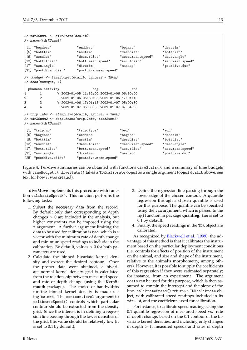
R> tdrXSumm1 <- diveStats(dcalib)
R> names(tdrXSumm1)
[1] "begdesc" "enddesc" "begasc" "desctim"
[5] "botttim" "asctim" "descdist" "bottdist"
[9] "ascdist" "desc.tdist" "desc.mean.speed" "desc.angle"
[13] "bott.tdist" "bott.mean.speed" "asc.tdist" "asc.mean.speed"
[17] "asc.angle" "divetim" "maxdep" "postdive.dur"
[21] "postdive.tdist" "postdive.mean.speed"
R> tbudget <- timeBudget(dcalib, ignoreZ = TRUE)
R> head(tbudget, 4)
phaseno activity beg end
1 1 W 2002-01-05 11:32:00 2002-01-06 06:30:00
2 2 L 2002-01-06 06:30:05 2002-01-06 17:01:10
3 3 W 2002-01-06 17:01:15 2002-01-07 05:00:30
4 4 L 2002-01-07 05:00:35 2002-01-07 07:34:00
R> trip.labs <- stampDive(dcalib, ignoreZ = TRUE)
R> tdrXSumm2 <- data.frame(trip.labs, tdrXSumm1)
R> names(tdrXSumm2)
[1] "trip.no" "trip.type" "beg" "end"
[5] "begdesc" "enddesc" "begasc" "desctim"
[9] "botttim" "asctim" "descdist" "bottdist"
[13] "ascdist" "desc.tdist" "desc.mean.speed" "desc.angle"
[17] "bott.tdist" "bott.mean.speed" "asc.tdist" "asc.mean.speed"
[21] "asc.angle" "divetim" "maxdep" "postdive.dur"
[25] "postdive.tdist" "postdive.mean.speed"
Figure 4: Per-dive summaries can be obtained with functions diveStats(), and a summary of time budgetswith timeBudget(). diveStats() takes a TDRcalibrate object as a single argument (object dcalib above, seetext for how it was created).
diveMove implements this procedure with func-tion calibrateSpeed(). This function performs thefollowing tasks:
1. Subset the necessary data from the record.By default only data corresponding to depthchanges > 0 are included in the analysis, buthigher constraints can be imposed using thez argument. A further argument limiting thedata to be used for calibration is bad, which is avector with the minimum rate of depth changeand minimum speed readings to include in thecalibration. By default, values > 0 for both pa-rameters are used.
2. Calculate the binned bivariate kernel den-sity and extract the desired contour. Oncethe proper data were obtained, a bivari-ate normal kernel density grid is calculatedfrom the relationship between measured speedand rate of depth change (using the KernS-mooth package). The choice of bandwidthsfor the binned kernel density is made us-ing bw.nrd. The contour.level argument tocalibrateSpeed() controls which particularcontour should be extracted from the densitygrid. Since the interest is in defining a regres-sion line passing through the lower densities ofthe grid, this value should be relatively low (itis set to 0.1 by default).
3. Define the regression line passing through thelower edge of the chosen contour. A quantileregression through a chosen quantile is usedfor this purpose. The quantile can be specifiedusing the tau argument, which is passed to therq() function in package quantreg. tau is set to0.1 by default.
4. Finally, the speed readings in the TDR object arecalibrated.
As recognized by Blackwell et al. (1999), the ad-vantage of this method is that it calibrates the instru-ment based on the particular deployment conditions(i.e. controls for effects of position of the instrumenton the animal, and size and shape of the instrument,relative to the animal’s morphometry, among oth-ers). However, it is possible to supply the coefficientsof this regression if they were estimated separately;for instance, from an experiment. The argumentcoefs can be used for this purpose, which is then as-sumed to contain the intercept and the slope of theline. calibrateSpeed() returns a TDRcalibrate ob-ject, with calibrated speed readings included in itstdr slot, and the coefficients used for calibration.
For instance, to calibrate speed readings using the0.1 quantile regression of measured speed vs. rateof depth change, based on the 0.1 contour of the bi-variate kernel densities, and including only changesin depth > 1, measured speeds and rates of depth
R News ISSN 1609-3631

Vol. 7/3, December 2007 14
change > 0:
R> vcalib <- calibrateSpeed(dcalib,
+ tau = 0.1, contour.level = 0.1,
+ z = 1, bad = c(0, 0),
+ cex.pts = 0.2)
Figure 5: The relationship between measured speedand rate of depth change can be used to calibratespeed readings. The line defining the calibrationfor speed measurements passes through the bottomedge of a chosen contour, extracted from a bivariatekernel density grid.
This call produces the plot shown in Figure 5,which can be suppressed by the use of the logical ar-gument plot. Calibrating speed readings allows forthe meaningful interpretation of further parameterscalculated by diveStats(), whenever a TDRspeedobject was found in the TDRcalibrate object:
• The total distance travelled, mean speed, anddiving angle during the descent and ascentphases of the dive.
• The total distance travelled and mean speedduring the bottom phase of the dive, and thepost-dive interval.
Summary
The diveMove package provides tools for analyz-ing diving behaviour, including convenient methodsfor the visualization of the typically large amountsof data collected by TDRs. The package’s mainstrengths are its ability to:
1. identify wet vs. dry periods,
2. calibrate depth readings,
3. identify individual dives and their phases,
4. summarize time budgets,
5. calibrate speed sensor readings, and
6. provide basic summaries for each dive identi-fied in TDR records.
Formal S4 classes are supplied to efficiently storeTDR data and results from intermediate analysis,making the retrieval of intermediate results readilyavailable for customized analysis. Development ofthe package is ongoing, and feedback, bug reports,or other comments from users are very welcome.
Acknowledgements
Many of the ideas implemented in this package de-veloped over fruitful discussions with my mentorsJohn P.Y. Arnould, Christophe Guinet, and EdwardH. Miller. I would like to thank Laurent Dubrocawho wrote draft code for some of diveMove’s func-tions. I am also greatly endebted to the regular con-tributors to the R-help newsgroup who helped mesolve many problems during development.
Bibliography
S. Blackwell, C. Haverl, B. Le Boeuf, and D. Costa. Amethod for calibrating swim-speed recorders. Ma-rine Mammal Science, 15(3):894–905, 1999.
Sebastián P. LuqueDepartment of Biology, Memorial UniversitySt. John’s, NL, [email protected]
R News ISSN 1609-3631

Vol. 7/3, December 2007 15
Very Large Numbers in R: IntroducingPackage BrobdingnagLogarithmic representation for floating-pointnumbers
Robin K. S. Hankin
Introduction
The largest floating point number representable instandard double precision arithmetic is a little un-der 21024, or about 1.79× 10308. This is too small forsome applications.
The R package Brobdingnag (Swift, 1726) over-comes this limit by representing a real number x us-ing a double precision variable with value log |x|,and a logical corresponding to x ≥ 0; the S4 classof such objects is brob. Complex numbers with largeabsolute values (class glub) may be represented us-ing a pair of brobs to represent the real and imagi-nary components.
The package allows user-transparent access tothe large numbers allowed by Brobdingnagian arith-metic. The package also includes a vignette—brob—which documents the S4 methods used and includesa step-by-step tutorial. The vignette also functions asa “Hello, World!” example of S4 methods as used ina simple package. It also includes a full descriptionof the glub class.
Package Brobdingnag in use
Most readers will be aware of a googol which is equalto 10100:
> require(Brobdingnag)
> googol <- as.brob(10)^100
[1] +exp(230.26)
Note the coercion of double value 10 to an ob-ject of class brob using function as.brob(): raisingthis to the power 100 (also double) results in anotherbrob. The result is printed using exponential nota-tion, which is convenient for very large numbers.
A googol is well within the capabilities of stan-dard double precision arithmetic. Now, however,suppose we wish to compute its factorial. Taking thefirst term of Stirling’s series gives
> stirling <- function(n) {
+ n^n * exp(-n) * sqrt(2 * pi * n)
+ }
which then yields
> stirling(googol)
[1] +exp(2.2926e+102)
Note the transparent coercion to brob formwithin function stirling().
It is also possible to represent numbers very closeto 1. Thus
> 2^(1/googol)
[1] +exp(6.9315e-101)
It is worth noting that if x has an exact repre-sentation in double precision, then ex is exactly rep-resentable using the system described here. Thus eand e1000 are represented exactly.
Accuracy
For small numbers (that is, representable using stan-dard double precision floating point arithmetic),Brobdingnag suffers a slight loss of precision com-pared to normal representation. Consider the follow-ing function, whose return value for nonzero argu-ments is algebraically zero:
f <- function(x){as.numeric( (pi*x -3*x -(pi-3)*x)/x)
}
This function combines multiplication and addi-tion; one might expect a logarithmic system such asdescribed here to have difficulty with it.
> f(1/7)
[1] 1.700029e-16
> f(as.brob(1/7))
[1] -1.886393e-16
This typical example shows that Brobdingnagiannumbers suffer a slight loss of precision for numbersof moderate magnitude. This degradation increaseswith the magnitude of the argument:
> f(1e+100)
[1] -2.185503e-16
> f(as.brob(1e+100))
[1] -3.219444e-14
Here, the brob’s accuracy is about two orders ofmagnitude worse than double precision arithmetic:this would be expected, as the number of bits re-quired to specify the exponent goes as log log x.
Compare
R News ISSN 1609-3631

Vol. 7/3, December 2007 16
> f(as.brob(10)^1000)
[1] 1.931667e-13
showing a further degradation of precision. How-ever, observe that conventional double precisionarithmetic cannot deal with numbers this big, andthe package returns about 12 correct significant fig-ures.
A practical example
In the field of population dynamics, and espe-cially the modelling of biodiversity (Hankin, 2007b;Hubbell, 2001), complicated combinatorial formulaeoften arise.
Etienne (2005), for example, considers a sampleof N individual organisms taken from some naturalpopulation; the sample includes S distinct species,and each individual is assigned a label in the range 1to S. The sample comprises ni members of species i,with 1 ≤ i ≤ S and ∑ ni = N. For a given sam-ple D, Etienne defines, amongst other terms, K(D, A)for 1 ≤ A ≤ N − S + 1 as
∑{a1 ,...,aS|∑S
i=1 ai=A}
S
∏i=1
s(ni , ai)s(ai , 1)s(ni , 1)
(1)
where s(n, a) is the Stirling number of the secondkind (Abramowitz and Stegun, 1965). The summa-tion is over ai = 1, . . . , ni with the restriction thatthe ai sum to A, as carried out by blockparts() ofthe partitions package (Hankin, 2006, 2007a).
Taking an intermediate-sized dataset due toSaunders1 of only 5903 individuals—a relativelysmall dataset in this context—the maximal elementof K(D, A) is about 1.435 × 101165. The accu-racy of package Brobdingnag in this context maybe assessed by comparing it with that computedby PARI/GP (Batut et al., 2000) with a work-ing precision of 100 decimal places; the naturallogs of the two values are 2682.8725605988689and 2682.87256059887 respectively: identical to 14significant figures.
Conclusions
The Brobdingnag package allows representationand manipulation of numbers larger than those cov-
ered by standard double precision arithmetic, al-though accuracy is eroded for very large numbers.This facility is useful in several contexts, includingcombinatorial computations such as encountered intheoretical modelling of biodiversity.
Acknowledgments
I would like to acknowledge the many stimulatingand helpful comments made by the R-help list overthe years.
Bibliography
M. Abramowitz and I. A. Stegun. Handbook of Mathe-matical Functions. New York: Dover, 1965.
C. Batut, K. Belabas, D. Bernardi, H. Cohen,and M. Olivier. User’s guide to pari/gp.Technical Reference Manual, 2000. url:http://www.parigp-home.de/.
R. S. Etienne. A new sampling formula for neutralbiodiversity. Ecology Letters, 8:253–260, 2005. doi:10.111/j.1461-0248.2004.00717.x.
R. K. S. Hankin. Additive integer partitions in R.Journal of Statistical Software, 16(Code Snippet 1),May 2006.
R. K. S. Hankin. Urn sampling without replacement:Enumerative combinatorics in R. Journal of Statisti-cal Software, 17(Code Snippet 1), January 2007a.
R. K. S. Hankin. Introducing untb, an R package forsimulating ecological drift under the Unified Neu-tral Theory of Biodiversity, 2007b. Under review atthe Journal of Statistical Software.
S. P. Hubbell. The Unified Neutral Theory of Biodiversityand Biogeography. Princeton University Press, 2001.
J. Swift. Gulliver’s Travels. Benjamin Motte, 1726.
W. N. Venables and B. D. Ripley. Modern AppliedStatistics with S-PLUS. Springer, 1997.
Robin K. S. HankinSouthampton Oceanography CentreSouthampton, United [email protected]
1The dataset comprises species counts on kelp holdfasts; here saunders.exposed.tot of package untb (Hankin, 2007b), is used.
R News ISSN 1609-3631
Vol. 7/3, December 2007 17
Applied Bayesian Non- andSemi-parametric Inference usingDPpackageby Alejandro Jara
Introduction
In many practical situations, a parametric model can-not be expected to describe in an appropriate man-ner the chance mechanism generating an observeddataset, and unrealistic features of some commonmodels could lead to unsatisfactory inferences. Inthese cases, we would like to relax parametric as-sumptions to allow greater modeling flexibility androbustness against misspecification of a parametricstatistical model. In the Bayesian context such flex-ible inference is typically achieved by models withinfinitely many parameters. These models are usu-ally referred to as Bayesian Nonparametric (BNP) orSemiparametric (BSP) models depending on whetherall or at least one of the parameters is infinity dimen-sional (Müller & Quintana, 2004).
While BSP and BNP methods are extremely pow-erful and have a wide range of applicability withinseveral prominent domains of statistics, they are notas widely used as one might guess. At least partof the reason for this is the gap between the type ofsoftware that many applied users would like to havefor fitting models and the software that is currentlyavailable. The most popular programs for Bayesiananalysis, such as BUGS (Gilks et al., 1992), are gener-ally unable to cope with nonparametric models. Thevariety of different BSP and BNP models is huge;thus, building for all of them a general softwarepackage which is easy to use, flexible, and efficientmay be close to impossible in the near future.
This article is intended to introduce an R pack-age, DPpackage, designed to help bridge the pre-viously mentioned gap. Although its name is mo-tivated by the most widely used prior on the spaceof the probability distributions, the Dirichlet Process(DP) (Ferguson, 1973), the package considers andwill consider in the future other priors on functionalspaces. Currently, DPpackage (version 1.0-5) allowsthe user to perform Bayesian inference via simula-tion from the posterior distributions for models con-sidering DP, Dirichlet Process Mixtures (DPM), PolyaTrees (PT), Mixtures of Triangular distributions, andRandom Bernstein Polynomials priors. The packagealso includes generalized additive models consider-ing penalized B-Splines. The rest of the article is or-ganized as follows. We first discuss the general syn-tax and design philosophy of the package. Next, themain features of the package and some illustrative
examples are presented. Comments on future devel-opments conclude the article.
Design philosophy and generalsyntax
The design philosophy behind DPpackage is quitedifferent from that of a general purpose language.The most important design goal has been the imple-mentation of model-specific MCMC algorithms. Adirect benefit of this approach is that the samplingalgorithms can be made dramatically more efficient.
Fitting a model in DPpackage begins with a callto an R function that can be called, for instance,DPmodel or PTmodel. Here “model" denotes a de-scriptive name for the model being fitted. Typically,the model function will take a number of argumentsthat govern the behavior of the MCMC sampling al-gorithm. In addition, the model(s) formula(s), data,and prior parameters are passed to the model func-tion as arguments. The common elements in anymodel function are:
i) prior: an object list which includes the valuesof the prior hyperparameters.
ii) mcmc: an object list which must include theintegers nburn giving the number of burn-in scans, nskip giving the thinning interval,nsave giving the total number of scans to besaved, and ndisplay giving the number ofsaved scans to be displayed on screen: the func-tion reports on the screen when every ndisplayscans have been carried out and returns theprocess’s runtime in seconds. For some spe-cific models, one or more tuning parameters forMetropolis steps may be needed and must beincluded in this list. The names of these tun-ing parameters are explained in each specificmodel description in the associated help files.
iii) state: an object list giving the current valuesof the parameters, when the analysis is the con-tinuation of a previous analysis, or giving thestarting values for a new Markov chain, whichis useful for running multiple chains startingfrom different points.
iv) status: a logical variable indicating whetherit is a new run (TRUE) or the continuation of aprevious analysis (FALSE). In the latter case the
R News ISSN 1609-3631

Vol. 7/3, December 2007 18
current values of the parameters must be spec-ified in the object state.
Inside the R model function the inputs to themodel function are organized in a more useableform, the MCMC sampling is performed by call-ing a shared library written in a compiled language,and the posterior sample is summarized, labeled, as-signed into an output list, and returned. The outputlist includes:
i) state: a list of objects containing the currentvalues of the parameters.
ii) save.state: a list of objects containing theMCMC samples for the parameters. Thislist contains two matrices randsave andthetasave which contain the MCMC samplesof the variables with random distribution (er-rors, random effects, etc.) and the parametricpart of the model, respectively.
In order to exemplify the extraction of the outputelements, consider the abstract model fit:
fit <- DPmodel(..., prior, mcmc,state, status, ....)
The lists can be extracted using the following code:
fit$statefit$save.state$randsavefit$save.state$thetasave
Based on these output objects, it is possible touse, for instance, the boa (Smith, 2007) or the coda(Plummer et al., 2006) R packages to perform con-vergence diagnostics. For illustration, we considerthe coda package here. It requires a matrix of pos-terior draws for relevant parameters to be saved asan mcmc object. As an illustration, let us assume thatwe have obtained fit1, fit2, and fit3, by indepen-dently running a model function three times, speci-fying different starting values each time. To computethe Gelman-Rubin convergence diagnostic statisticfor the first parameter stored in the thetasave object,the following commands may be used,
library("coda")chain1 <- mcmc(fit1$save.state$thetasave[,1])chain2 <- mcmc(fit2$save.state$thetasave[,1])chain3 <- mcmc(fit3$save.state$thetasave[,1])coda.obj <- mcmc.list(chain1 = chain1,
chain2 = chain2,chain3 = chain3)
gelman.diag(coda.obj, transform = TRUE)
where the fifth command saves the results as an ob-ject of class mcmc.list, and the sixth command com-putes the Gelman-Rubin statistic from these threechains.
Generic R functions such as print, plot,summary, and anova have methods to display the re-sults of the DPpackage model fit. The function print
displays the posterior means of the parameters inthe model, and summary displays posterior summarystatistics (mean, median, standard deviation, naivestandard errors, and credibility intervals). By de-fault, the function summary computes the 95% HPDintervals using the Monte Carlo method proposed byChen & Shao (1999). Note that this approximation isvalid when the true posterior distribution is symmet-ric. The user can display the order statistic estimatorof the 95% credible interval by using the followingcode,
summary(fit, hpd=FALSE)
The plot function displays the trace plots and akernel-based estimate of the posterior distributionfor the model parameters. Similarly to summary, theplot function displays the 95% HPD regions in thedensity plot and the posterior mean. The same plotbut considering the 95% credible region can be ob-tained by using,
plot(fit, hpd=FALSE)
The anova function computes simultaneous cred-ible regions for a vector of parameters from theMCMC sample using the method described by Be-sag et al. (1995). The output of the anova function isan ANOVA-like table containing the pseudo-contourprobabilities for each of the factors included in thelinear part of the model.
Implemented Models
Currently DPpackage (version 1.0-5) contains func-tions to fit the following models:
i) Density estimation: DPdensity, PTdensity,TDPdensity, and BDPdensity using DPM ofnormals, Mixtures of Polya Trees (MPT),Triangular-Dirichlet, and Bernstein-Dirichletpriors, respectively. The first two functions al-low uni- and multi-variate analysis.
ii) Nonparametric random effects distributions inmixed effects models: DPlmm and DPMlmm, us-ing a DP/Mixtures of DP (MDP) and DPMof normals prior, respectively, for the linearmixed effects model. DPglmm and DPMglmm, us-ing a DP/MDP and DPM of normals prior,respectively, for generalized linear mixed ef-fects models. The families (links) implementedby these functions are binomial (logit, probit),poisson (log) and gamma (log). DPolmm andDPMolmm, using a DP/MDP and DPM of nor-mals prior, respectively, for the ordinal-probitmixed effects model.
iii) Semiparametric IRT-type models: DPraschand FPTrasch, using a DP/MDP and fi-nite PT (FPT)/MFPT prior for the Rasch
R News ISSN 1609-3631

Vol. 7/3, December 2007 19
model with a binary distribution, respectively.DPraschpoisson and FPTraschpoisson, em-ploying a Poisson distribution.
iv) Semiparametric meta-analysis models: DPmetaand DPMmeta for the random (mixed) effectsmeta-analysis models, using a DP/MDP andDPM of normals prior, respectively.
v) Binary regression with nonparametric link:CSDPbinary, using Newton et al. (1996)’s cen-trally standardized DP prior. DPbinary andFPTbinary, using a DP and a finite PT prior forthe inverse of the link function, respectively.
vi) AFT model for interval-censored data:DPsurvint, using a MDP prior for the errordistribution.
vii) ROC curve estimation: DProc, using DPM ofnormals.
viii) Median regression model: PTlm, using amedian-0 MPT prior for the error distribution.
ix) Generalized additive models: PSgam, using pe-nalized B-Splines.
Additional tools included in the package areDPelicit, to elicit the DP prior using the exact andapproximated formulas for the mean and variance ofthe number of clusters given the total mass parame-ter and the number of subjects (see, Jara et al. 2007);and PsBF, to compute the Pseudo-Bayes factors formodel comparison.
Examples
Bivariate Density Estimation
As an illustration of bivariate density estimationusing DPM normals (DPdensity) and MPT models(PTdensity), part of the dataset in Chambers et al.(1983) is considered. Here, n = 111 bivariate obser-vations yi = (yi1, yi2)T on radiation yi1 and the cuberoot of ozone concentration yi2 are modeled. Theoriginal dataset has the additional variables windspeed and temperature. These were analyzed byMüller et al. (1996) and Hanson (2006).
The DPdensity function considers the multivari-ate extension of the univariate Dirichlet Process Mix-ture of Normals model discussed in Escobar & West(1995),
yi | G iid∼∫
Nk (µ, Σ) G(dµ, dΣ)
G | M, G0 ∼ DP (αG0)
G0 ≡ Nk(µ | m1 ,κ−10 Σ)IWk (Σ | ν1 , Ψ1)
α ∼ Γ (a0 , b0)
m1 | m2 , S2 ∼ Nk (m2 , S2)
κ0 | τ1 , τ2 ∼ Γ (τ1/2, τ2/2)
Ψ1 | ν2 , Ψ2 ∼ IWk (ν2 , Ψ2)
where Nk (µ, Σ) refers to a k-variate normal distri-bution with mean and covariance matrix µ and Σ,respectively, IWk (ν, Ψ) refers to an inverted-Wishartdistribution with shape and scale parameter ν and Ψ,respectively, and Γ (a, b) refers to a gamma distribu-tion with shape and rate parameter, a and b, respec-tively. Note that the inverted-Wishart prior is param-eterized such that its mean is given by 1
ν−k−1 Ψ−1.The PTdensity function considers a Mixture of
multivariate Polya Trees model discussed in Hanson(2006),
yi|Giid∼ G, (1)
G | α, µ, Σ, M ∼ PTM(Πµ,Σ ,Aα), (2)
p(µ, Σ) ∝ |Σ|−(d+1)/2 , (3)
α|a0 , b0 ∼ Γ(a0 , b0), (4)
where the PT prior is centered around a Nk(µ, Σ)distribution. To fit these models we used the follow-ing commands:
# Datadata("airquality")attach(airquality)ozone <- Ozone**(1/3)radiation <- Solar.R
# Prior informationpriorDPM <- list(a0 = 1, b0 = 1/5,nu1 = 4, nu2 = 4,s2 = matrix(c(10000,0,0,1),ncol = 2),m2 = c(180,3),psiinv2 = matrix(c(1/10000,0,0,1),ncol = 2),tau1 = 0.01, tau2 = 0.01)
priorMPT <- list(a0 = 5, b0 = 1, M = 4)
# MCMC parametersmcmcDPM <- list(nburn = 5000, nsave = 20000,
nskip = 20, ndisplay = 1000)
mcmcMPT <- list(nburn = 5000, nsave = 20000,nskip = 20, ndisplay = 1000,tune1 = 0.025, tune2 = 1.1,tune3 = 2.1)
# Fitting the modelsfitDPM <- DPdensity(y = cbind(radiation,ozone),
prior = priorDPM,mcmc = mcmcDPM,state = NULL,status = TRUE,na.action = na.omit)
R News ISSN 1609-3631

Vol. 7/3, December 2007 20
fitMPT <- PTdensity(y = cbind(radiation,ozone),prior = priorMPT,mcmc = mcmcMPT,state = NULL,status = TRUE,na.action = na.omit)
We illustrate the results from these analyses inFigure 1. This figure shows the contour plots ofthe posterior predictive density for each model.
radiation
ozon
e
0 100 200 300
12
34
56
●●
●
●
●
●
●
●
●
●
●
●
●
●
●
●
●
●
●
●
●
●
●
●
●
●
●
●●
●
●
●●
●
●
●
●
●
●
●●
●
●
●
●
●
●
●
●
●
●
●
●
●
●
●
●
●●
●
●
●
●
●
●
●
●
●
●
●
●
●
●
●
●
●
●
●●
●
●●
●
●●
●
●
●
●●
●●
●
●
●
●
●
●
●
●
●
●
●
●
●
●
●
●
●
●●
(a)
radiation
ozon
e
0 100 200 300
12
34
56
●●
●
●
●
●
●
●
●
●
●
●
●
●
●
●
●
●
●
●
●
●
●
●
●
●
●
●●
●
●
●●
●
●
●
●
●
●
●●
●
●
●
●
●
●
●
●
●
●
●
●
●
●
●
●
●●
●
●
●
●
●
●
●
●
●
●
●
●
●
●
●
●
●
●
●●
●
●●
●
●●
●
●
●
●●
●●
●
●
●
●
●
●
●
●
●
●
●
●
●
●
●
●
●
●●
(b)
Figure 1: Density estimate for the New York AirQuality Measurements dataset, using (a) DPdensityand (b) PTdensity, respectively.
Figure 1 clearly shows a departure from the nor-mality assumption for these data. The results indi-cate the existence of at least two clusters of data. Werefer to Hanson (2006) for more details and compar-isons between these models.
Interval-Censored Data
The DPsurvint function implements the algorithmdescribed by Hanson & Johnson (2004) for semipara-metric accelerated failure time (AFT) models. We il-lustrate the function on a dataset involving time tocosmetic deterioration of the breast for women with
stage 1 breast cancer who have undergone a lumpec-tomy, for two treatments, these being radiation, andradiation coupled with chemotherapy. Radiation isknown to cause retraction of the breast, and there issome evidence that chemotherapy worsens this ef-fect. There is interest in the cosmetic impact of thetreatments because both are considered very effec-tive in preventing recurrence of this early stage can-cer.
The data come from a retrospective study of 46patients who received radiation only and 48 who re-ceived radiation plus chemotherapy. Patients wereobserved typically every four to six months and ateach observation a clinician recorded the level ofbreast retraction that had taken place since the lastvisit: none, moderate, or severe. The time-to-eventconsidered was the time until moderate or severebreast retraction, and this time is interval censoredbetween patient visits or right censored if no breastretraction was detected over the study period of 48months. As the observed intervals were the resultof pre-scheduled visits, an independent noninforma-tive censoring process can be assumed. The datawere analyzed by Hanson & Johnson (2004) and alsogiven in Klein & Moeschberger (1997).
In the analysis of survival data with covari-ates, the semiparametric proportional hazards (PH)model is the most popular choice. It is flexible andeasily fitted using standard software, at least forright-censored data. However, the assumption ofproportional hazard functions may be violated andwe may seek a proper alternative semiparametricmodel. One such model is the AFT model. Whereasthe PH model assumes the covariates act multiplica-tively on a baseline hazard function, the AFT modelassumes that the covariates act multiplicatively onthe argument of the baseline survival distribution, G,P(T > t | x) = G
((t exp{xT
i β}, +∞)), thus provid-
ing a model with a simple interpretation of the re-gression coefficients for practitioners.
Classical treatments of the semiparametric AFTmodel with interval-censored data were presented,for instance, in Lin & Zhang (1998). Note, how-ever, that for semiparametric AFT models there isnothing comparable to a partial likelihood function.Therefore, the vector of regression coefficients andthe baseline survival distribution must be estimatedsimultaneously, complicating matters enormously inthe interval-censored case. The more recent classicalapproaches only provide inferences about the regres-sion coefficients and not for the survival function.
In the Bayesian semiparametric context, Chris-tensen & Johnson (1998) assigned a simple DP prior,centered in a single distribution, to baseline survivalfor nested interval-censored data. A marginal like-lihood for the vector of regression coefficients β ismaximized to provide a point estimate and resultingsurvival curves. However, this approach does notallow the computation of credible intervals for the
R News ISSN 1609-3631

Vol. 7/3, December 2007 21
parameters. Moreover, it may be difficult in prac-tice to specify a single centering distribution for theDP prior and, once specified, a single centering dis-tribution may affect inferences. To overcome thesedifficulties, a MDP prior can be considered. Underthis approach, it is not very difficult to demonstratedthat the computations involved for a full Bayesiansolution are horrendous at best, even for the non-censored data problem. The analytic intractabilityof the Bayesian semiparametric AFT model has beenovercome using MCMC methods by Hanson & John-son (2004).
To test whether chemotherapy in addition to ra-diotherapy has an effect on time to breast retraction,an AFT model Ti = exp(−xT
i β)Vi, i = 1, . . . , n, wasconsidered. We model the baseline distribution inthe AFT model using a MDP prior centered in a stan-dard parametric family, the lognormal distribution,
V1 , . . . , Vn|Giid∼ G,
G | α, µ,σ2 ∼ DP (αG0) , G0 ≡ LN(µ,σ2),
µ | m0 , s0 ∼ N (m0 , s0) ,
σ−2 | τ1 , τ2 ∼ Γ (τ1/2, τ2/2) ,
β | β0 , Sβ0∼ Np
(β0 , Sβ0
),
where LN(m, s2) and N
(m, s2) refer to a log-normal
and normal distribution, respectively, with locationm and scale parameter s2. The precision parameterof the MDP prior was chosen to be α = 10, allowingfor moderate deviations from the log-normal family.We allow the parametric family to hold only approx-imately, and the resulting model is robust againstmis-specification of the baseline survival distribu-tion. The covariate of interest is trti = 0 if the ithpatient had radiotherapy only and trti = 1 if theith patient had radiotherapy and chemotherapy. Thefollowing commands were used to fit the model,
# Datadata("deterioration")attach(deterioration)y <- cbind(left,right)
# MCMC parametersmcmc <- list(nburn = 20000, nsave = 10000,
nskip = 20, ndisplay = 1000,tune = 0.25)
# Prior informationprior <- list(alpha = 10, beta0 = rep(0,1),
Sbeta0 = diag(100,1), m0 = 0,s0 = 1, tau1 = 0.01, tau2 = 0.01)
# Fitting the modelfit <- DPsurvint(y ~ trt, prior = prior,
mcmc = mcmc, state = NULL,status = TRUE)
In our analysis, the posterior mean and 95% HPDassociated with trt was 0.50 (0.12, 0.82), indicatingthat including chemotherapy significantly reducesthe time to deterioration. Figure 2 (page 22) displaysposterior summary statistics for the parameters of in-terest. In this case, the output includes the log of theConditional Predictive Ordinate (CPO) (see, Geisser& Eddy 1979) for each data point, the AFT regressioncoefficients, the parameters of the DP centering dis-tribution, and the number of clusters.
Inferences about the survival curves can be ob-tained from the MCMC output. Indeed, givena sample of the parameters of size J, a sam-ple of the survival curve for a given x can bedrawn as follows: for the MCMC scan j of theposterior distribution, with j = 1, . . . , J, wesample from S( j)(t|x, data) ∼ Beta(a( j)(t), b( j)(t))where a( j)(t) = α( j)G( j)
0
((t exp(xTβ( j)), +∞)
)+ ∑
ni=1 δ
V( j)i
((t exp(xTβ( j)), +∞)
), and b( j)(t) =
α( j) + N − a( j)(t). This approach is implemented inthe function predict.DPsurvint. For user-specifiedvalues of the covariates, xnew, and the grid where thesurvival function is evaluated, grid, posterior infor-mation for the survival curves can be obtained usingthe following commands,
xnew <- matrix(c(0,1), nrow=2, ncol=1)grid <- seq(0.01,70,1)pred <- predict(fit, xnew=xnew, grid=grid)plot(pred, all=FALSE, band=TRUE)
The resulting survival curves and point-wise 95%HPD intervals are given in Figure 3 (page 23).
Semiparametric Generalized Linear MixedModel
Lesaffre & Spiessens (2001) analyzed data from amulticentre randomized comparison of two oraltreatments for toe-nail infection (dermatophyte ony-chomycosis) involving two groups of 189 patientsevaluated at seven visits; on week 0, 4, 8, 12, 24, 36,and 48. Onychomycosis, known popularly as toe-nail fungus, is a fairly common condition that notonly can disfigure and sometimes destroy the nailbut that also can lead to social and self-image is-sues for sufferers. Onychomycosis can be caused byseveral types of fungi known as dermatophytes, aswell as by non-dermatophytic yeasts or molds. Der-matophyte onychomycosis corresponds to the typecaused by dermatophytes. Here we are interestedin the degree of onycholysis which expresses the de-gree of separation of the nail plate from the nail-bedand which was scored in four categories (0, absent;1, mild; 2, moderate; 3, severe). These data wereanalyzed by Lesaffre & Spiessens (2001) using gen-eralized estimating equations (GEE) and generalizedlinear mixed models (GLMM).
R News ISSN 1609-3631

Vol. 7/3, December 2007 22
> summary(fit)
Bayesian Semiparametric AFT Regression Model
Call:
DPsurvint.default(formula = y ~ trt, prior = prior, mcmc = mcmc,
state = state, status = TRUE)
Posterior Predictive Distributions (log):
Min. 1st Qu. Median Mean 3rd Qu. Max.
-4.5920 -2.3570 -1.4600 -1.6240 -0.7121 -0.1991
Regression coefficients:
Mean Median Std. Dev. Naive Std.Error 95%HPD-Low 95%HPD-Upp
trt 0.502282 0.513219 0.195521 0.001955 0.120880 0.820614
Baseline distribution:
Mean Median Std. Dev. Naive Std.Error 95%HPD-Low 95%HPD-Upp
mu 3.255374 3.255518 0.173132 0.001731 2.917770 3.589759
sigma2 1.021945 0.921764 0.469061 0.004691 0.366900 1.908676
Precision parameter:
Mean Median Std. Dev. Naive Std.Error 95%HPD-Low 95%HPD-Upp
ncluster 27.58880 28.00000 3.39630 0.03396 20.00000 33.00000
Acceptance Rate for Metropolis Step = 0.2637435
Number of Observations: 94
Figure 2: Posterior summary for the Breast Cancer Data fit using DPsurvint.
GLMM provide a popular framework for theanalysis of longitudinal measures and clustered data.The models account for correlation among clusteredobservations by including random effects in the lin-ear predictor component of the model. AlthoughGLMM fitting is typically complex, standard ran-dom intercept and random intercept/slope modelswith normally distributed random effects can nowbe routinely fitted in standard software. Such mod-els are quite flexible in accommodating heterogenousbehavior, but they suffer from the same lack of ro-bustness against departures from distributional as-sumptions as other statistical models based on Gaus-sian distributions.
A common strategy for guarding against suchmis-specification is to build more flexible distribu-tional assumptions for the random effects into themodel. Following Lesaffre & Spiessens (2001), weconsider a logistic mixed effects model to examinethe probability of moderate or severe toenail separa-tion Y = 1 versus the probability of absent or mildY = 0, including as covariates treatment (trt) (0 or1), time (t) (continuous), and time×treatment inter-action,
logit{
P(
Yi j = 1 | β,θi
)}= θi + β1Trti + β2Timei j +
β3Trti × Timei j .
However, we replace the normality assumption ofthe random intercepts by using a DPM of normals
prior (see, e.g., Müller et al. 2007),
θi | G iid∼ G,
G | P, Σk ∼∫
N(m, Σk)P(dm),
P | α, µ, Σ ∼ DP (αN(µ, Σ)) ,
β ∼ Np(β0 , Sβ0
),
Σk | ν0 , T ∼ IWk (ν0 , T) ,
µ | mb , Sb ∼ Nq (mb , Sb) ,
Σ | ν0 , Tb ∼ IWk (νb , Tb) ,
α | a0 , b0 ∼ Γ (a0 , b0) .
The semiparametric GLMM using DPM of normalsmodel can be fitted using function DPMglmm and thefollowing code,
# MCMC parametersmcmc <- list(nburn = 20000, nsave = 20000,
nskip = 50, ndisplay = 1000)
# Prior informationprior <- list(a0 = 2.01, b0 = 0.01,
nu0 = 2.05, tinv = diag(0.02,1),nub = 2.05, tbinv = diag(0.02,1),mb = rep(0,1), Sb = diag(100,1),beta0 = rep(0,3),
R News ISSN 1609-3631

Vol. 7/3, December 2007 23
Sbeta0 = diag(100,3))
# Fitting the modelfitDPM <- DPMglmm(fixed = infect~trt+
time*trt, random = ~ 1|idnr,family = binomial(logit),prior = prior, mcmc = mcmc,state = NULL, status = TRUE)
0 10 20 30 40 50 60 70
0.0
0.2
0.4
0.6
0.8
1.0
Time
Sur
viva
l
(a)
0 10 20 30 40 50 60 70
0.0
0.2
0.4
0.6
0.8
1.0
Time
Sur
viva
l
(b)
Figure 3: Breast cancer data: Posterior probabilityof no evidence of breast retraction for (a) radiother-apy only and (b) radiotherapy plus chemotherapy,respectively.
Figure 4 shows the posterior estimate of therandom effects distribution. The predictive den-sity is overlaid on a plot of the posterior meansof the random effects. The results clearly in-dicate departure from the normality assumption,suggesting the existence of groups of patientswith respect to the resistance against the infection.
−15 −10 −5 0 5 10 15
0.00
0.05
0.10
0.15
values
dens
ity
●●●● ●●●● ●●●●● ●●●● ●●●●● ●●●● ●● ●● ●●● ●●● ●●● ●●●●●● ●●●●●●● ●●●●●●●●●● ●●●● ● ● ●●● ●●●●● ●● ●● ● ●●● ●●● ●● ●● ●●●● ●● ●●●●● ●●●●●●●●●●●● ●●●● ●● ●● ● ●●● ● ●● ●●●●●● ●●● ●●●●● ●●●● ●●● ●● ●●● ●●●●● ●● ●●●● ●●●● ●●●●●● ●●●●● ●● ●●● ●●● ●● ● ●●●●● ● ●● ●●●●●● ●●● ●●● ● ●● ●●●● ● ●● ●● ●● ●●●●●●● ●● ●●● ●● ●●● ●●●●●●●● ●●● ●● ●● ●●●●●● ●●● ●●● ● ● ●●● ●● ●●●●●●●●●● ●● ●●●●●
Figure 4: Toe-nail data: Random effects distributionand posterior means estimated using DPMglmm.
Figure 5 (page 24) reports summary statistics forthe posterior distribution of the parameters of in-terest. It includes posterior means and 95% HPDintervals for the parameters along with two modelperformance measures: DIC and LPML. DIC is thedeviance information criterion of Spiegelhalter et al.(2002). LPML is the log pseudo marginal likelihoodof Geisser & Eddy (1979), which is a leave-one-outcross validatory measure based on predictive densi-ties. A parametric analysis of these data (not shown),considering equivalent prior distributions, gave aDIC and LPML of 964.2 and -484.0, respectively. Theresults, therefore, indicate that the DPM version ofthe model outperforms the normal model using ei-ther the LPML or DIC statistic, suggesting that thesemiparametric model is better both for explainingthe observed data and from a predictive point ofview.
Figure 5 (page 24) and the Pseudo Contour prob-abilities of the covariates in the model (see below)suggest a significant effect of time on the degree oftoe-nail infection. As expected because of random-ization of the patients to the treatment groups, no sig-nificant difference between the two treatment groupsat baseline was observed. The results also suggesta non-significant difference in the evolution in timebetween the treatment groups, contradicting the re-sults under the parametric normal model. The pos-terior mean (95% HPD interval) for β3 (Trt × Time)under the normal assumption for the random effectswas −0.138 (−0.271; −0.005). These results illus-trate the consequences of the incorrect use of tradi-tional model assumptions in the GLMM context.
> anova(fitDPM)Table of Pseudo Contour Probabilities
Response: infectDf PsCP
trt 1 0.512time 1 <0.01 ***
R News ISSN 1609-3631

Vol. 7/3, December 2007 24
> summary(fitDPM)
Bayesian semiparametric generalized linear mixed effect model
Call:
DPMglmm.default(fixed = infect ~ trt + time * trt, random = ~1 |
idnr, family = binomial(logit), prior = prior, mcmc = mcmc,
state = state, status = TRUE)
Posterior Predictive Distributions (log):
Min. 1st Qu. Median Mean 3rd Qu. Max.
-9.644e+00 -2.335e-01 -4.190e-02 -2.442e-01 -8.629e-03 -4.249e-05
Model's performance:
Dbar Dhat pD DIC LPML
753.0 603.6 149.4 902.5 -466.0
Regression coefficients:
Mean Median Std. Dev. Naive Std.Error 95%HPD-Low 95%HPD-Upp
(Intercept) -2.508419 -2.440589 0.762218 0.005390 -4.122867 -1.091684
trt 0.300309 0.304453 0.478100 0.003381 -0.669604 1.242553
time -0.392343 -0.390384 0.046101 0.000326 -0.482329 -0.302442
trt:time -0.128891 -0.128570 0.072272 0.000511 -0.265813 0.018636
Kernel variance:
Mean Median Std. Dev. Naive Std.Error 95%HPD-Low 95%HPD-Upp
sigma-(Intercept) 0.0318682 0.0130737 0.0966504 0.0006834 0.0009878 0.1069456
Baseline distribution:
Mean Median Std. Dev. Naive Std.Error 95%HPD-Low 95%HPD-Upp
mub-(Intercept) -2.624227 -2.558427 1.405269 0.009937 -5.621183 0.008855
sigmab-(Intercept) 26.579978 23.579114 13.640300 0.096451 7.714973 52.754246
Precision parameter:
Mean Median Std. Dev. Naive Std.Error 95%HPD-Low 95%HPD-Upp
ncluster 70.6021 64.0000 36.7421 0.2598 11.0000 143.0000
alpha 38.4925 25.7503 44.1123 0.3119 1.1589 112.1120
Acceptance Rate for Metropolis Steps = 0.8893615 0.9995698
Number of Observations: 1908
Number of Groups: 294
Figure 5: Posterior summary for the Toe-nail Data fit using DPMglmm.
trt:time 1 0.075 .---Signif. codes: 0 '***' 0.001 '**' 0.01'*' 0.05 '.' 0.1 ' ' 1
Finally, information about the posterior distributionof the subject-specific effects can be obtained by us-ing the DPMrandom function as follows,
> DPMrandom(fitDPM)
Random effect information for the DP object:
Call:DPMglmm.default(fixed = infect ~ trt +
time * trt, random = ~1 |idnr,family = binomial(logit),
prior = prior, mcmc = mcmc,state = state, status = TRUE)
Posterior mean of subject-specific components:
(Intercept)1 1.6239
.
.383 2.0178
R News ISSN 1609-3631

Vol. 7/3, December 2007 25
Summary and Future Develop-ments
As the main obstacle for the practical use of BSPand BNP methods has been the lack of estimationtools, we presented an R package for fitting some fre-quently used models. Until the release of DPpack-age, the two options for researchers who wished tofit a BSP or BNP model were to write their own codeor to rely heavily on particular parametric approxi-mations to some specific processes using the BUGScode given in Peter Congdon’s books (see, e.g., Con-gdon 2001). DPpackage is geared primarily towardsusers who are not willing to bear the costs associatedwith both of these options.
Many improvements to the current status of thepackage can be made. For example, all DPpackagemodeling functions compute CPOs for model com-parison. However, only some of them compute theeffective number of parameters pD and the devianceinformation criterion (DIC), as presented by Spiegel-halter et al. (2002). These and other model compar-ison criteria will be included for all the functions infuture versions of DPpackage.
The implementation of more models, the devel-opment of general-purpose sampling functions, andthe ability to run several Markov chains at once andto handle large dataset problems through the use ofsparse matrix techniques, are areas of further im-provement.
Acknowledgments
I wish to thank (in alphabetical order) Timothy Han-son, George Karabatsos, Emmanuel Lesaffre, PeterMüller, and Fernando Quintana for many valuablediscussions, comments, and suggestions during thedevelopment of the package. Timothy Hanson andFernando Quintana are also co-authors of the func-tions PTdensity and FPTbinary, and BDPdensity, re-spectively. I gratefully acknowledge the partial sup-port of the KUL-PUC bilateral (Belgium-Chile) grantNo BIL05/03 and of the IAP research network grantNo P6/03 of the Belgian government (Belgian Sci-ence Policy). The author thanks Novartis, Belgium,for permission to use their dermatological data forstatistical research.
Bibliography
J. Besag, P. Green, D. Higdon, and K. Mengersen.Bayesian computation and stochastic systems(with Discussion). Statistical Science, 10:3–66, 1995.
J. M. Chambers, S. Cleveland, and A. P. Tukey.Graphical Methods for Data Analysis. Boston,USA: Duxbury, 1983.
M. H. Chen and Q. M. Shao. Monte Carlo estimationof Bayesian credible and HPD intervals. Journalof Computational and Graphical Statistics, 8(1):69–92,1999.
R. Christensen and W. O. Johnson. Modeling Ac-celerated Failure Time With a Dirichlet Process.Biometrika, 75:693–704, 1998.
P. Congdon. Bayesian Statistical Modelling. New York,USA: John Wiley and Sons, 2001.
M. D. Escobar and M. West. Bayesian density esti-mation and inference using mixtures. Journal of theAmerican Statistical Association, 90:577–588, 1995.
T. S. Ferguson. A Bayesian analysis of some nonpara-metric problems. The Annals of Statistics, 1:209–230,1973.
S. Geisser and W. Eddy. A predictive approach tomodel selection. Journal of the American StatisticalAssociation, 74:153–160, 1979.
W. R. Gilks, A. Thomas, and D. J. Spiegelhalter. Soft-ware for Gibbs sampler Computing Science andStatistics 24:439–448, 1992.
T. Hanson. Inference for Mixtures of Finite Polya TreeModels. Journal of the American Statistical Associa-tion, 101:1548–1565, 2006.
T. Hanson and W. O. Johnson. A Bayesian Semipara-metric AFT Model for Interval-Censored Data.Journal of Computational and Graphical Statistics13(2):341–361, 2004.
A. Jara, M. J. Garcia-Zattera, and E. Lesaffre. ADirichlet Process Mixture model for the analysis ofcorrelated binary responses. Computational Statis-tics and Data Analysis, 51:5402–5415, 2007.
J. Klein and M. Moeschberger. Survival Analysis. NewYork, USA: Springer-Verlag, 1997.
E. Lesaffre and B. Spiessens. On the effect of thenumber of quadrature points in a logistic random-effects model: an example. Applied Statistics 50:325–335, 2001.
G. Lin and C. Zhang. Linear Regression With Inter-val Censored Data. The Annals of Statistics 26:1306–1327, 1998.
P. Müller and F.A. Quintana. NonparametricBayesian Data Analysis. Statistical Science 19(1):95–110, 2004.
P. Müller, A. Erkanli, and M. West. BayesianCurve Fitting Using Multivariate Normal Mix-tures. Biometrika, 83:67–79, 1996.
P. Müller, F. A. Quintana, and G. Rosner. Semi-parametric Bayesian Inference for Multilevel Re-peated Measurement Data. Biometrics, 63(1):280–289, 2007.
R News ISSN 1609-3631
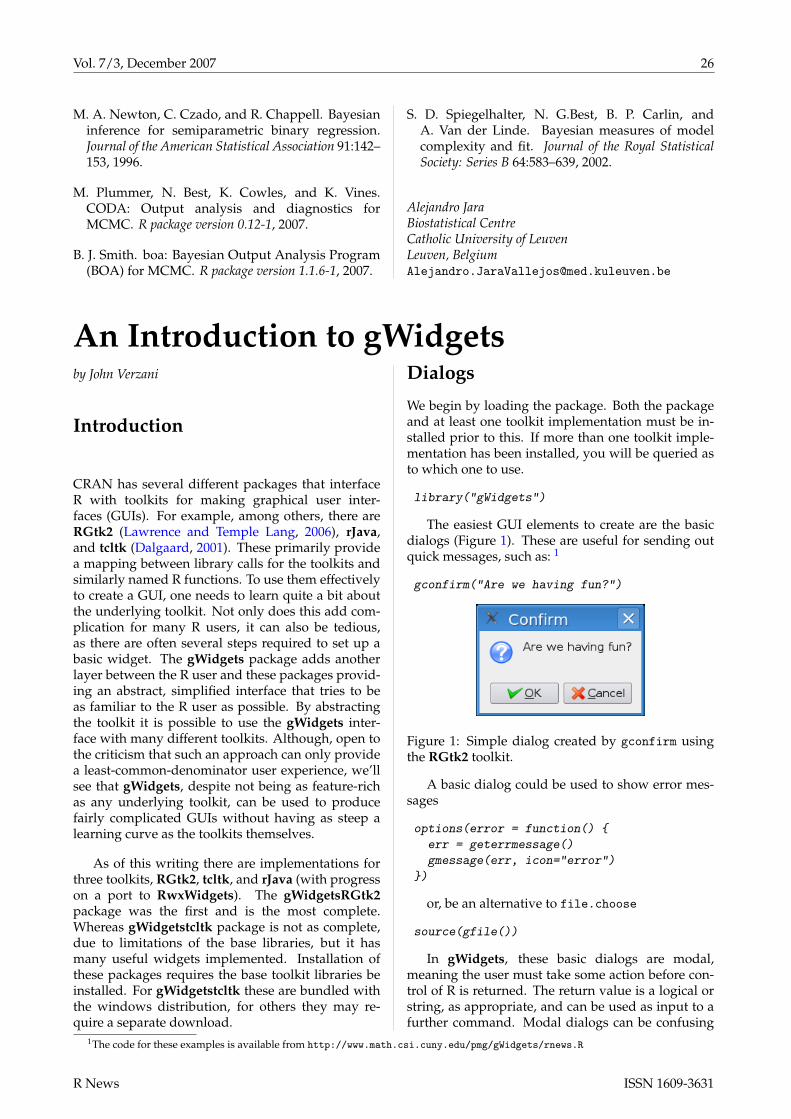
Vol. 7/3, December 2007 26
M. A. Newton, C. Czado, and R. Chappell. Bayesianinference for semiparametric binary regression.Journal of the American Statistical Association 91:142–153, 1996.
M. Plummer, N. Best, K. Cowles, and K. Vines.CODA: Output analysis and diagnostics forMCMC. R package version 0.12-1, 2007.
B. J. Smith. boa: Bayesian Output Analysis Program(BOA) for MCMC. R package version 1.1.6-1, 2007.
S. D. Spiegelhalter, N. G.Best, B. P. Carlin, andA. Van der Linde. Bayesian measures of modelcomplexity and fit. Journal of the Royal StatisticalSociety: Series B 64:583–639, 2002.
Alejandro JaraBiostatistical CentreCatholic University of LeuvenLeuven, [email protected]
An Introduction to gWidgetsby John Verzani
Introduction
CRAN has several different packages that interfaceR with toolkits for making graphical user inter-faces (GUIs). For example, among others, there areRGtk2 (Lawrence and Temple Lang, 2006), rJava,and tcltk (Dalgaard, 2001). These primarily providea mapping between library calls for the toolkits andsimilarly named R functions. To use them effectivelyto create a GUI, one needs to learn quite a bit aboutthe underlying toolkit. Not only does this add com-plication for many R users, it can also be tedious,as there are often several steps required to set up abasic widget. The gWidgets package adds anotherlayer between the R user and these packages provid-ing an abstract, simplified interface that tries to beas familiar to the R user as possible. By abstractingthe toolkit it is possible to use the gWidgets inter-face with many different toolkits. Although, open tothe criticism that such an approach can only providea least-common-denominator user experience, we’llsee that gWidgets, despite not being as feature-richas any underlying toolkit, can be used to producefairly complicated GUIs without having as steep alearning curve as the toolkits themselves.
As of this writing there are implementations forthree toolkits, RGtk2, tcltk, and rJava (with progresson a port to RwxWidgets). The gWidgetsRGtk2package was the first and is the most complete.Whereas gWidgetstcltk package is not as complete,due to limitations of the base libraries, but it hasmany useful widgets implemented. Installation ofthese packages requires the base toolkit libraries beinstalled. For gWidgetstcltk these are bundled withthe windows distribution, for others they may re-quire a separate download.
Dialogs
We begin by loading the package. Both the packageand at least one toolkit implementation must be in-stalled prior to this. If more than one toolkit imple-mentation has been installed, you will be queried asto which one to use.
library("gWidgets")
The easiest GUI elements to create are the basicdialogs (Figure 1). These are useful for sending outquick messages, such as: 1
gconfirm("Are we having fun?")
Figure 1: Simple dialog created by gconfirm usingthe RGtk2 toolkit.
A basic dialog could be used to show error mes-sages
options(error = function() {
err = geterrmessage()
gmessage(err, icon="error")
})
or, be an alternative to file.choose
source(gfile())
In gWidgets, these basic dialogs are modal,meaning the user must take some action before con-trol of R is returned. The return value is a logical orstring, as appropriate, and can be used as input to afurther command. Modal dialogs can be confusing
1The code for these examples is available from http://www.math.csi.cuny.edu/pmg/gWidgets/rnews.R
R News ISSN 1609-3631

Vol. 7/3, December 2007 27
if the dialog gets hidden by another window. Addi-tionally, modal dialogs disrupt a user’s flow. A moretypical GUI will allow the R session to continue andwill only act when a user initiates some action withthe GUI by mouse click, text entry, etc. The GUI de-signer adds handlers to respond to these events. ThegWidgets programming interface is based around fa-cilitating the following basic tasks in building a GUI:constructing widgets that a user can control to af-fect the state of the GUI, using generic functions toprogrammatically manipulate these widgets, simpli-fying the layout of widgets within containers, and fa-cilitating the assigning of handlers to events initiatedby the user of the GUI.
Selecting a CRAN site
Figure 2: GUI to select a CRAN mirror shown usinggWidgetstcltk. The filter feature of gtable has beenused to narrow the selection to USA sites. Doubleclicking a row causes the CRAN repository to be set.
Selecting an item from a list of items or a tableof items is a very common task in GUIs. Our nextexample presents a GUI that allows a user to se-lect with the mouse a CRAN repository from a ta-ble. The idea comes from a tcltk GUI created by thechooseCRANmirror function. This example showshow the widget constructors allow specification ofboth containers and event handlers.
We will use this function to set the CRAN reposi-tory from a URL.
setCRAN <- function(URL) {
repos = getOption("repos")
repos["CRAN"] <- gsub("/$", "", URL)
options(repos=repos)
}
To begin our GUI we first create a top-level win-dow to contain our table widget.
win <- gwindow("Select a CRAN mirror")
A call to gwindow will pop-up a new window on thescreen and return an object which can be manipu-lated later. The argument sets the window title.
The widget we create will show the possibleCRAN values in a tabular format for easy selectionby a mouse. Selection occurs when a row is clicked.We will assign this function to respond to a doubleclick event:
handler = function(h,...) {
URL <- svalue(tbl) # get value of widget
setCRAN(URL) # set URL
dispose(win) # close window
}
The svalue function is a new generic function whichretrieves the selected value for a widget, in this caseone called tbl constructed below. The dispose func-tion is a new generic which for windows causes themto be destroyed. So this handler will set the chosenURL and then destroy the top-level window.
The gtable function constructs a widget allow-ing the user to select a value from a data frame andreturns an object for which generic functions are de-fined. The row of the value is selected with a mouseclick, whereas, the selected column is specified at thetime the widget is constructed using the chosencolargument. Additionally, this function allows thespecification of a column whose unique values canbe used to filter the display of possible values to se-lect from.
tbl <- gtable(
items=utils:::getCRANmirrors(),
chosencol=4,
filter.column=2,
container=win,
handler=handler
)
Figure 2 shows the final widget using the tcltktoolkit.
Using gWidgets
We now go through the basic steps of building a GUIusing gWidgets a little more systematically.
Containers
As illustrated previously a top-level window is cre-ated using gwindow. The gWidgets package only al-lows one widget to be packed into a top-level win-dow. As such, typically a container that can holdmore than one object is packed into the top-level win-dow. There are several types of containers available.
R News ISSN 1609-3631
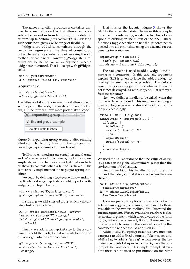
Vol. 7/3, December 2007 28
The ggroup function produces a container thatmay be visualized as a box that allows new wid-gets to be packed in from left to right (the default)or from top to bottom (horizontal=FALSE). Nestingsuch containers gives a wide range of flexibility.
Widgets are added to containers through thecontainer argument at the time of construction(which hereafter we shorten to cont) or using the addmethod for containers. However, gWidgetstcltk re-quires one to use the container argument when awidget is constructed. That is, except with gWidget-stcltk
win <- gwindow("test")
b <- gbutton("click me", cont=win)
is equivalent to
win <- gwindow("test")
add(win, gbutton("click me"))
The latter is a bit more convenient as it allows one tokeep separate the widget’s construction and its lay-out, but the former allows more portability of code.
Figure 3: Expanding group example after resizingwindow. The button, label and text widgets usenested ggroup containers for their layout.
To illustrate nested ggroup containers and the addand delete generics for containers, the following ex-ample shows how to create a widget that can hideor show its contents when a button is clicked. Thisis more fully implemented in the gexpandgroup con-tainer.
We begin by defining a top-level window and im-mediately add a ggroup instance which packs in itswidgets from top to bottom.
win <- gwindow("Expanding group")
g <- ggroup(horizontal=FALSE, cont=win)
Inside of g we add a nested group which will con-tain a button and a label.
g1 <- ggroup(horizontal=TRUE, cont=g)
button <- gbutton("V",cont=g1)
label <- glabel("Expand group example",
cont=g1)
Finally, we add a ggroup instance to the g con-tainer to hold the widgets that we wish to hide andput a widget into the new container.
g2 <- ggroup(cont=g, expand=TRUE)
e <- gedit("Hide this with button",
cont=g2)
That finishes the layout. Figure 3 shows theGUI in the expanded state. To make this exampledo something interesting, we define functions to re-spond to clicking on the button or the label. Thesefunctions toggle whether or not the g2 container ispacked into the g container using the add and deletegenerics for containers.
expandGroup = function()
add(g,g2, expand=TRUE)
hideGroup = function() delete(g,g2)
The add generic is used to add a widget (or con-tainer) to a container. In this case, the argumentexpand=TRUE is given to force the added widget totake up as much space as possible. The deletegeneric removes a widget from a container. The wid-get is not destroyed, as with dispose, just removedfrom its container.
Next, we define a handler to be called when thebutton or label is clicked. This involves arranging ameans to toggle between states and to adjust the but-ton text accordingly.
state <- TRUE # a global
changeState <- function(h,...) {
if(state) {
hideGroup()
svalue(button) <- ">"
} else {
expandGroup()
svalue(button) <- "V"
}
state <<- !state
}
We used the <<- operator so that the value of stateis updated in the global environment, rather than theenvironment of the handler.
Finally, we bind this handler to both the but-ton and the label, so that it is called when they areclicked.
ID <- addHandlerClicked(button,
handler=changeState)
ID <- addHandlerClicked(label,
handler=changeState)
There are just a few options for the layout of wid-gets within a ggroup container, compared to thoseavailable in the various toolkits. We illustrated theexpand argument. With rJava and tcltk there is alsoan anchor argument which takes a value of the formc(x,y) where x or y are −1, 0, or 1. These are usedto specify which corner of the space allocated by thecontainer the widget should add itself in.
Additionally, the ggroup instances have methodsaddSpace to add a fixed amount of blank space andaddSpring to add a “spring” which forces the re-maining widgets to be pushed to the right (or the bot-tom) of the containers. This simple example showshow these can be used to put buttons on the right
R News ISSN 1609-3631

Vol. 7/3, December 2007 29
side of a dialog. First we pack a ggroup instance intoa top-level container.
Figure 4: Illustration of addSpace and addSpringmethods of ggroup using the gWidgetsRGTk2 pack-age after resizing main window. The buttons arepushed to the right side by addSpring.
win <- gwindow("Mock up")
bg <- ggroup(cont=win, expand=TRUE)
addSpring(bg) # push to right
Now we add two buttons and a bit of space, 10pixels, between them. By default, packing is donefrom left to right, starting on the left. The use ofaddSpring pushes the packed in containers and wid-gets to the right side of the container.
b1 <- gbutton("cancel", cont=bg)
addSpace(bg,10) # add some space
b2 <- gbutton("ok", cont=bg)
The expand=TRUE value for bg ensures that thatcontainer expands to fill the space it can, otherwisethe button widgets would push to the boundary ofthe button group and not the outside container win.Figure 4 shows the widget.
Other containers are illustrated in the examplesbelow. These include glayout for laying out widgetsin a grid, gnotebook for holding multiple widgets atonce with tabs used to select between the widgets,and gpanedgroup which uses a movable pane to al-locate space between widgets. Additionally, gframeis similar to ggroup, but with an external frame andarea for a label.
Basic widgets
A GUI is composed of widgets packed into con-tainers. In gWidgets there are a number of famil-iar widgets. We’ve illustrated labels and buttons(glabel and gbutton). Additionally there are wid-gets to select from a list of items (gradio, gdroplist,and gcheckboxgroup); widgets to select from a ta-ble of values (gtable); widgets to select files ordates (gfile, gcalendar); widgets to edit text (gedit,gtext); a widget to edit a data frame (gdf); a widgetto display graphic files (gimage); and others. Not allare available for each toolkit.
The following example, modified from a recent RNews article on the rpanel package (Bowman et al.,2006), illustrates how many of these widgets can becombined to create a GUI to demonstrate confidenceintervals. This example uses the glayout containerto lay out its widgets in a grid.
First we pack the container into a top level win-dow.
win <- gwindow("CI example")
tbl <- glayout(cont=win)
The glayout container uses matrix-like notation tospecify where the widgets are placed. When the as-signed value is a string, a glabel is used.
Figure 5: GUI for a confidence interval demonstra-tion, using gWidgetsrJava, illustrating several dif-ferent widgets: gedit for single-line editing; andgdroplist, gslider, gspinbox, and gradio for selec-tion from a fixed set of items.
tbl[1,1] <- "mu"
tbl[1,2] <-
(mu <- gedit("0", cont=tbl,
coerce.with=as.numeric))
tbl[2,1] <- "sigma"
tbl[2,2] <-
(sigma <- gdroplist(c(1,5,10),
cont=tbl))
tbl[3,1] <- "n"
tbl[3,2] <- (
n <- gslider(from=5,to=100, by=1,
value = 10, cont=tbl))
tbl[4,1] <- "conf. level"
tbl[4,2, expand=TRUE] <-
(confLevel <- gspinbutton(
from=0.5, to=0.99, by=0.01,
value=0.95, cont=tbl))
tbl[5,1] <- "No. intervals"
tbl[5,2] <-
(noIntervals <- gradio(c(10,25,
50,100), cont=tbl))
tbl[6,2] <-
(resample <- gbutton("resample",
cont=tbl))
visible(tbl) <- TRUE
The last line with visible is necessary for gWidget-sRGtk2 to produce the layout.
The matrix-notation refers to where the widget isplaced. An assignment like
tbl[1:2,2:3] <- "testing"
would place a label within the area for the first andsecond rows and second and third columns. Unlikematrices, the notation is not used to vectorize theplacement of several widgets, extract widgets, or re-place a widget. The above code completes the widget
R News ISSN 1609-3631

Vol. 7/3, December 2007 30
construction and layout. Figure 5 shows a realizationusing rJava.
The widgets have various arguments to specifytheir values that depend on what the widget does.For example, the slider and spinbutton select a valuefrom a sequence, so the arguments mirror those ofseq. Some widgets have a coerce.with argumentwhich allows a text-based widget, like gedit, to re-turn numeric values through svalue. The gdroplistwidget is used above to pop up its possible valuesfor selection. Additionally, if the editable=TRUE ar-gument is given, it becomes a combo-box allowing auser to input a different value.
In Figure 5 we see in the slider widget one of thelimitations of the gWidgets approach – it is not asfeature rich as any individual toolkit. Although theunderlying JSlider widget has some means to adjustthe labels on the slider, gWidgets provides none in itsAPI, which in this case is slightly annoying, as Java’schosen values of 5, 28, 51, 74, and 97 just don’t seemright.
The values specified by these widgets are to befed into the function makeCIs, which is not shownhere, but uses matplot to construct a graphic dis-playing simulated confidence intervals. To make thisGUI interactive, the following handler will be usedto respond to changes in the GUI. We need to callsvalue on each of the widgets and then pass theseresults to the makeCIs function. This task is stream-lined by using lapply and do.call:
allWidgets <- list(mu,sigma,noIntervals,
n, confLevel, resample)
plotCI <- function(h, ...) {
lst <- lapply(allWidgets,svalue)
do.call(makeCIs,lst)
}
Again we use lapply to add the handler to re-spond to the different widget default events all atonce.
invisible(sapply(allWidgets,function(i)
addHandlerChanged(i,handler=plotCI))
)
Interacting with widgets programmati-cally
In gWidgets, the widget and container constructorsreturn S4 objects of various classes. These objects areaccessed programmatically with generic functions.As was sensible, generic methods familiar to R userswere used, and when not possible, new genericswere added. For example, for widgets which storevalues to select from, the generics [ and [<- are usedto refer to the possible values. For other widgets, asappropriate, the generics dim, names, length, etc., aredefined. To get and set a widget’s “selected” value,the new generic functions svalue and svalue<-were
defined. The term “selected” is loosely defined, e.g.,applying to a button’s text when clicked.
This simple example shows how selecting valuesin a checkbox group can be used to set the possiblevalues in a drop list. First we create a container tohold the two widgets.
win <- gwindow("methods example")
g <- ggroup(cont=win)
The construction of the two widgets is straight-forward: simply specify the available values usingitems.
cb <- gcheckboxgroup(items=letters[1:5],
cont=g)
dl <- gdroplist(items="", cont=g)
To finish, the following adds a handler to cbwhich will update the possible values of dl when theuser changes the value of the checkbox group.
ID <- addHandlerChanged(cb,
function(h,...) {
dl[] <- svalue(cb)
})
A few other new generics are defined in gWid-gets for the basic widgets such as font<- for settingfont properties, size<- to adjust the size in pixels fora widget, enabled<- to adjust if the widget can ac-cept input, and the pair tag and tag<-, which is likeattr only its values are stored with the widget. Thislatter function is useful as its values can be updatedwithin a function call, such as a handler, as this nextexample shows. The expanding group example withthe state variable would have been a good place touse this feature.
> x = gbutton("test", cont=gwindow())
> tag(x,"ex") <- attr(x,"ex") <- "a"
> f = function(y)
+ tag(y,"ex") <- attr(y,"ex") <- "b"
> c(tag(x,"ex"),attr(x,"ex"))
[1] "a" "a"
> f(x)
> c(tag(x,"ex"),attr(x,"ex"))
[1] "b" "a"
Handlers
A GUI user initiates an event to happen when a but-ton is clicked, or a key is pressed, or a drag and dropis initiated, etc. The gWidgets package allows one tospecify a handler, or callback, to be called when anevent occurs. These handlers may be specified whena widget is constructed using the handler argument,or added at a later time. To add the default handler,use the addHandlerChanged generic. Most, but notall, widgets have just one type of event for whicha handler may be given. For instance, the gedit
R News ISSN 1609-3631

Vol. 7/3, December 2007 31
widget has the default handler respond to the eventof a user pressing the ENTER key. Whereas, theaddHandlerKeystroke method can be used to add ahandler that responds to any keystroke. Officially,only one handler can be assigned per event, althoughsome toolkits allow more.
Handlers return an ID which can be used withremoveHandler to remove the response to the event.
The signature of a handler function has a first ar-gument, h, to which is passed a list containing com-ponents obj, action and perhaps others. The objcomponent refers to the underlying widget. In theexamples above we found this widget after storingit to a variable name, this provides an alternative.The action component may be used to passed alongan arbitrary value to the handler. The other compo-nents depend on the widget. For the ggraphics wid-get (currently just gWidgetsRGtk2), the componentsx and y report the coordinates of a mouse click foraddHandlerClicked. Whereas, for addDropTargetthe dropdata component contains a string specifyingthe value being dragged.
To illustrate the drag-and-drop handlers the fol-lowing creates two buttons. The drop source needs ahandler which returns the value passed along to thedropdata component of the drop target handler. Inthis example, clicking on the first button and drag-ging its value onto the label will change the text dis-played on the label.
g = ggroup(cont=gwindow("DnD example"))
l1 <- gbutton("drag me", cont=g)
l2 <- glabel("drop here", cont=g)
ID <- addDropSource(l1, handler=
function(h,...) svalue(h$obj))
ID <- addDropTarget(l2, handler =
function(h,...)
svalue(h$obj) <- h$dropdata)
Drag and drop works with all the toolkits exceptgWidgetsrJava where only what is provided nativelythrough the Java libraries is working.
An application
This last example shows how to make a more am-bitious GUI for a task; in this case, an interface todownload and visualize stock prices. New widgetsand containers shown are the toolbar widget; thenotebook container, which is used to present dif-ferent simultaneous summaries of a stock; the vari-able selector widget, for selecting variables fromthe workspace; and the generic widget constructor,which creates a simple GUI based on a function’s ar-guments, as found by formal. Although more in-volved than the examples above, it is meant to showhow specialized GUIs can be formed relatively eas-ily by gluing together the pieces available throughgWidgets. Figure 6 shows the result of running the
following code, then downloading data for Googleinto the session.
Figure 6: Stock browser widget using gWidget-sRGtk2. This illustrates a toolbar, the variable selec-tor, and a notebook container.
We begin by loading the tseries package whichcontains the get.hist.quote() function for retriev-ing stock data from www.yahoo.com and calls in thehandy zoo package by Achim Zeileis and GaborGrothendieck or use for later use.
invisible(require("tseries"))
In previous examples we used the global environ-ment to store our variables. This works well for asingle GUI, but can quickly lead to problems withcolliding variable names with multiple GUIs. Settingup a separate environment for each GUI is one wayaround this potential conflict. Similarly, the protopackage can be used effectively to provide an envi-ronment and more. Other possible methods are touse namespaces or the environment within a func-tion body. In this example, we create a new environ-ment to store our global variables.
e <- new.env()
The environment e is accessed using list-like syntax.To download stock information we use
get.hist.quote. We define this function to reducethe number of arguments so that ggenericwidgetproduces a simpler GUI (Figure 7).
getQuotes = function(
inst = "GOOG",
quote = c("Open","High","Low","Close"),
start, end)
get.hist.quote(inst, start=start,
end=end, quote=quote)
R News ISSN 1609-3631

Vol. 7/3, December 2007 32
Figure 7: The GUI for getQuotes created byggenericwidget using the RGtk2 toolkit.
We define two functions to display graphicalsummaries of the stock, using the zoo package toproduce the plots. Rather than use a plot device (asonly gWidgetsRGtk2 implements an embeddableone through ggraphics), we choose instead to makea file containing the plot as a graphic and displaythis using the gimage widget. In gWidgetstcltk thenumber of graphic formats that can be displayed islimited, so we use an external program, convert, tocreate a gif file. This is not needed if using RGtk2 orrJava.
showTrend <- function(stock) {
trendPlotFile <- e$trendPlotFile
png(trendPlotFile)
plot(stock, main="Trend plot")
lines(rollmean(stock, k = 30), lwd=2,
lty=2, col=gray(.7))
lines(rollmean(stock, k = 90), lwd=2,
lty=3, col=gray(.7))
legend(index(stock)[length(stock)],
min(stock),
legend=c("30 day MA","90 day MA"),
lty=2:3,xjust=1, yjust=0)
dev.off()
## create a gif file
system(paste("convert ",
trendPlotFile," ",
trendPlotFile,".gif",sep=""))
svalue(e$trendPlot) = paste(
trendPlotFile,".gif",sep="")
}
The function showDiscount is similarly definedbut not shown.
The main function below is used to update thenotebook pages when a new stock is selected, orthe graphing parameters are changed. This func-tion refers to widgets defined in a subsequent codechunk.
updateNB <- function(h,...) {
## update data set
ifelse(e$curDSName != "",
e$curDS <- get(e$curDSName),
return())
## get data within specified range
start <- svalue(e$startD)
if(start == "") start=NULL
end <- svalue(e$endD)
if(end == "") end = NULL
dataSet = window(e$curDS,
start=start,end=end)
## update summaries
svalue(e$noSum) =
capture.output(summary(dataSet))
showDiscount(dataSet,
svalue(e$discRate))
showTrend(dataSet)
}
Now the main application is defined. First somevariables.
e$curDSName <- ""
e$curDS <- NA
e$tsPlotFile <- tempfile()
e$trendPlotFile <- tempfile()
Next we define the main window and a containerto hold the subsequent widgets.
## layout
e$win <- gwindow("Stock browser")
e$gp <- ggroup(horizontal=FALSE,
cont=e$win)
The first widget will be a toolbar. This basic onehas two actions, one to open a dialog allowing a userto download stock information from the internet, theother a quit button. To be more friendly to R users,The gtoolbar() constructor uses a list to specify thetoolbar structure, rather than, say, XML. Basically,each named component of this list should be a listwith a handler component and optionally an iconcomponent. Menubars are similarly defined, onlynesting is allowed.
## Set up simple toolbar
tb <- list()
tb$"Get quotes"$handler <- function(...)
ggenericwidget("getQuotes",
container=gwindow("Get quotes"))
tb$"Get quotes"$icon <- "ts"
tb$Quit$handler <- function(...)
dispose(e$win)
tb$Quit$icon <- "cancel"
theTB <- gtoolbar(tb, cont=e$gp)
This application has widgets to adjust the interestrate (used as a discounting factor), and the start andend dates. The date widgets use the gcalendar()constructor for easier date selection.
## Now add parameters
e$pg <- ggroup(horizontal=TRUE,
cont = e$gp)
## the widgets
l <- glabel("Discount rate (%):",
cont=e$pg)
e$discRate <- gedit(0, cont=e$pg,
R News ISSN 1609-3631

Vol. 7/3, December 2007 33
coerce.with=as.numeric,
handler=updateNB)
e$pg <- ggroup(horizontal=TRUE,
cont = e$gp)
l <- glabel("Range of dates:",
cont=e$pg)
curDate <- Sys.Date()
l <- glabel("from=", cont=e$pg)
e$startD <-
gcalendar(as.character(curDate-365),
handler=updateNB, cont=e$pg)
l <- glabel("to=", cont=e$pg)
e$endD <-
gcalendar(as.character(curDate),
handler=updateNB, cont=e$pg)
A paned group is used for the final layout, alllow-ing the user to adjust the amount of room for eachmajor part of the GUI. One part is a variable selectionwidget provided by gvarbrowser(). Double clickinga row calls the updateNB handler to update the note-book pages.
e$gpg <- gpanedgroup(cont=e$gp,
expand=TRUE)
e$varSel <- gvarbrowser(
cont= e$gpg,
handler = function(h,...) {
e$curDSName <- svalue(e$varSel)
updateNB()
})
The other major part of the GUI is a notebook con-tainer to hold the three different summaries of thestock.
e$nb <- gnotebook(cont=e$gpg)
Finally, we add pages to the notebook containerbelow. The additional label argument sets the textfor the tab. (These can be adjusted later usingnames<-.)
## A numeric summary of the data set
e$noSum <- gtext("Numeric summary",
cont=e$nb, label="Summary")
## First graphic summary
e$tsPlot <- gimage(e$tsPlotFile,
cont=e$nb, label="Time series plot")
size(e$tsPlot) <- c(480,480)
## secondGraphicSummary
e$trendPlot <- gimage(e$trendPlotFile,
cont=e$nb, label="Trend plot")
Acknowledgments
The gWidgets package was designed as an extensionof the iWidgets package (Urbanek, 2007) of SimonUrbanek for Michael Lawrence’s RGtk2 package (anextension of Duncan Temple Lang’s RGtk package).Michael had done an initial port. Philippe Grosjeansuggested to the author to abstract the code to makeit independent of toolkit and Simon Urbanek con-tributed several key ideas for this. The author wouldlike to thank all of the above for helpful comments,and the thoughtful and thorough report of an anony-mous referee of an initial version of this article.
Bibliography
A. Bowman, E. Crawford, and R. Bowman. rpanel:Making graphs move with tcltk. R News, 6(5):12–17, October 2006.
P. Dalgaard. The R-Tcl/Tk interface. In F. Leisch andK. Hornik, editors, Proceedings of the 2nd Interna-tional Workshop on Distributed Statistical Computing(DSC 2001), March 2001. ISSN: 1609-395X.
M. Lawrence and D. Temple Lang. RGTK2–A GUI Toolkit for R. Statistical Computingand Graphics, 17(1), 2006. Pusblished athttp://www.amstat-online.org/sections/graphics/newsletter/newsletter.html.
S. Urbanek. iWidgets. http://www.rforge.net/iWidgets/.
John VerzaniThe College of Staten IslandCity University of New [email protected]
R News ISSN 1609-3631

Vol. 7/3, December 2007 34
Financial Journalism with RBill Alpert
R proved itself a sharp tool in testing the stock picksof Jim Cramer, a popular US financial journalist.We examined Cramer’s advice for a recent coverstory in Barron’s, the Dow Jones & Co. stock marketweekly, where I am a reporter and floundering R user(Alpert, 2007). The August 20, 2007 story should beaccessible without subscription at the Barron’s web-site (http://www.barrons.com).
The 52-year-old Cramer once ran a hedge fundwhich racked up 24% annualized returns over abouta dozen years. His current celebrity comes from theMad Money television show on the cable networkCNBC, in which he makes Buy and Sell recommen-dations to the accompaniment of wacky sound ef-fects and clownish antics. A few have attemptedto measure the performance of modest samples ofCramer’s picks (Engelberg et al., 2007; Nayda, 2006).Yet Cramer makes almost 7,000 recommendationsa year, according to the count of a database at hisMad Money website (http://madmoney.thestreet.com/). He has never reported the performance of allthose stock picks. I figured I’d try.
As in most projects, data collection was the hardpart. I called Cramer and asked for any records of hisMad Money picks. After ripping into me and all jour-nalists who’ve reviewed his show, he stopped tak-ing my calls. Meanwhile, I found a website main-tained by a retired stock analyst, who had talliedabout 1,300 of Cramer’s Mad Money recommenda-tions over two years. I also found the abovemen-tioned database at Cramer’s official website, whichrecorded over 3,400 recommendations from the pre-ceding six months. This Cramer site classified hispicks in ways useful for subsetting in R, but con-spicuously lacked any performance summaries. Iturned these Web records of his stock picks into Ex-cel spreadsheets. Then I downloaded stock price his-tories from Edgar Online’s I-Metrix service (http://I-Metrix.Edgar-Online.com), using some Excelmacros. None of this was trivial work, because Iwanted a year’s worth of stock prices around eachrecommendation and the date ranges varied over thethousands of stocks. Financial data suppliers can de-liver a wealth of information for a single, commondate range, but an "event study" like mine involvedhundreds of date ranges for thousands of stocks.Most finance researchers deal with this hassle by us-ing SAS and a third-party add-on called Eventus thateases data collection. But I wanted to use R.
I reached out to quantitative finance program-mer Pat Burns and Pat wrote some R code for ourevent study style analysis. Pat has posted his ownworking paper on our study at his website (http://www.burns-stat.com). R’s flexibility was useful
because we needed a novel data structure for theCramer analysis. In most analyses, the data for prices(or for returns) are in a matrix where each column is adifferent stock and each row is a specific date. In ourcase, each stock recommendation had the same num-ber of data points, so a matrix was a logical choice.However, instead of each row being a specific date, itwas a specific offset from the recommendation date.We still needed the actual date, though, in order toget the difference in return between the stocks andthe S&P 500 on each day – to see if Cramer’s picks"beat the market." Pat’s solution was to have a ma-trix of dates as a companion to the matrix of prices.It was then a trivial subscripting exercise to get a ma-trix of S&P returns that matched the matrix of returnsfor the recommendations. Many stocks were recom-mended multiple times, so the column names of thematrices were not unique.
Once the data were in R, it was fairly easyto test various investment strategies, such as buy-ing the day after Cramer’s 6 pm show or, instead,waiting two days before buying. Any investmentstrategy that actively picks stocks should at leastbeat the returns you’d get from a passive market-mimicking portfolio with comparable risk (that is,similar return variance) – and it should beat themarket by enough to cover trading costs. Oth-erwise you ought to keep your money in an in-dex fund. You can see the importance of market-adjusting Cramer’s returns by comparing the redand blue lines in Figure 1. The Nasdaq Compos-ite Index is arguably a better match to the riski-ness of Cramer’s widely-varying returns. We madehis performance look better when we used the S&P.
Figure 1: Average cumulative percentage log returnfrom the day of broadcast for approx. 1,100 MadMoney recommendations recorded at http://www.yourmoneywatch.com. Blue line shows return rela-tive to S&P 500 Index.
The red line shows his average pick’s unad-justed log return, while the blue shows the log re-
R News ISSN 1609-3631

Vol. 7/3, December 2007 35
turn relative to the Standard & Poors 500 Index.The data were roughly 1,100 Buy recommendationsover the period from July 2005 to July 2007. Thelines’ lefthand peaks mark the trading day after eachevening broadcast, when enthusiastic fans have bidup Cramer’s pick. We ultimately tested severaldozen investment strategies.
The results were disappointing for someone whowants to follow Cramer’s advice. You could notbeat the market by a statistically significant amount ifyou followed his recommendations in any way read-ily available to a viewer. But we did find that youmight make an interesting return if you went againstCramer’s recommendations – shorting his Buys themorning after his shows, while putting on offset-ting S&P 500 positions. This shorting opportunityappears in Figure 1, as the widening difference be-tween the red and blue lines. If a viewer shorted onlyCramer’s recommendations that jumped 2% or moreon the day after his broadcasts, that difference couldearn the viewer an annualized 12% on average (lesstrading costs). The bootstrapped 95% confidence in-tervals of this difference ranged from 3% to 21%. (Forbackground on bootstrap techniques, see Efron andTibshirani, 1993)
0 5 10 15 20 25 30
−4
−3
−2
−1
0
Negative lightning
Days
Cum
ulat
ive
abno
rmal
ret
urn
Figure 2: Cumulative log return relative to S&P500 on about 480 of Cramer’s off-the-cuff LightningRound Sell recommendations, as recorded at mad-money.thestreet.com. The yellow band is a boot-strapped 95% confidence interval, showing that thenegative return – desirable for Sell recommendations– is clearly different from zero
One reason we tested so many different strate-gies is that when I finally started getting responsesfrom Cramer and CNBC, they kept changing theirstory. They argued about selection. Neither of mydatabases were reliable records of Cramer’s picks,CNBC said, not even the database endorsed by
Cramer at his website. Instead of giving me a recordof his two-years’ of stock picks, they suggested thatI watch tapes of all his shows, which they’d gladlyprovide me. It reminded me of the endless tasks as-signed in fairy tales – separating peas from the ashpile.
They also argued that certain subsets of Cramer’srecommendations were the only proper ones tocount . . . as if viewers would somehow know whichof his screaming "Buys" he meant them to ignore.As it happened, the segment of his show thatCramer argued most shrilly for us to deselect (the"Lightning Round" with his impromptu responses tophoned-in questions) was the only segment with anystatistically-significant marketbeating returns – inthis case, on the Sell recommendations (see Figure 2).Embarrassingly, the Sell recommendations thatCramer prepared in advance went up (see Figure 3).
0 5 10 15 20 25 30
−2
−1
01
2
Negative featured or discussed
Days
Cum
ulat
ive
abno
rmal
ret
urn
Figure 3: Cumulative log return relative to S&P 500on about 160 of Cramer’s Prepared Sell recommen-dations as recorded at madmoney.thestreet.com
CNBC and Cramer also kept shifting their claimabout when Cramer advises his audience to act onhis picks. After I told Cramer that viewers gotmarket-lagging returns if they bought the day afterhis recommendations (when most viewers clearly dotheir buying), he angrily said that he "always" ad-vises waiting until the second day. When I cameback with evidence that a second-day purchase alsolagged the market (as is clear in Figure 1), CNBCsaid that Cramer’s advice had "always" been to waita week or two after each show. Later still, they saidthat a good test should wait exactly five days.
Such data dredging and methodological de-bates are probably not unfamiliar to readers of thisnewsletter who use R for high stakes evaluationsof pharmaceuticals or government interventions, butjournalism may be extreme in its extensive interac-
R News ISSN 1609-3631

Vol. 7/3, December 2007 36
tion with the subjects of its analyses. Academicsrarely contact authors they critique – indeed, post-publication data repositories aim to make it easy toreplicate a study without questioning the authors.Good journalists do the opposite: we contact the sub-jects of our investigations early and often.
And of course, R let us flexibly change our anal-ysis every time CNBC and Cramer changed theirstory. When they argued for a different selection,R made it easy to create a new data subset. Whenthey argued for a different holding strategy, R’s in-dexing facility let us start and stop our analysis ondifferent dates. In fact, when I begged CNBC fortheir own analysis of Cramer’s performance, theysaid something that should warm the hearts of allyou folks who’ve made R the powerful environmentit is. CNBC told me not to expect a timely responsefrom them because it was obvious that Pat and I hadspent months on our analysis. In truth, Pat put in lessthan a week’s work.
Acknowledgments
Essential services for this project included: R cod-ing by Pat Burns, of Burns Statistics in London; Excel
macros by Edgar Online analyst Elias-John Kies andfrom Tufts University undergraduate Madison Mc-gaffin; wise statistical pointers from Tim Hesterberg,of Insightful Corp. in Seattle . . . none of whom bearresponsibility for any woebegone errors.
Bibliography
B. Alpert. Shorting Cramer. Barron’s, 2007.
B. Efron and R. Tibshirani. Introduction to the Boot-strap. Chapman and Hall, 1993.
J. Engelberg, C. Sasseville, and J. Williams. Attentionand Asset Prices: the Case of Mad Money. Tech-nical report, Kellogg School of Management, 2007.http://papers.ssrn.com.
N. Nayda. You! Me! Let’s Get Ready to Make MadMoney!!! Technical report, Elmont Virginia Ele-mentary School, 2006. Science fair project.
Bill AlpertBarron’s, Dow Jones & Co., [email protected]
Need A Hint?Sanford Weisberg and Hadley Wickham
Suppose you have created an object in R, for examplefrom a regression fit using lm or loess. You knowthat auxiliary functions exist that do useful compu-tations on the object, but you can’t remember theirnames. You need a hint on what to do next.
The hints function in the hints package does justthis, finding a list of appropriate functions to jogyour memory. For example, Figure 1 shows a list ofhints for a lm object.
The output lists methods for generic functionslike print specific to the class you specify, as wellas searching the documentation to find all mentionsof the class. You can then use the usual help mecha-nism to learn more about each of these methods andfunctions.
The hints function has three arguments:
hints(x, class=class(x), all.packages=FALSE)
If specified, the argument x can be any R object. Forexample, x might have been created by x <- lm(yz). hints determines the S3 class of the object, andthen looks for functions that operate on that class.The S3 class of an object is a character vector, andmay consist of multiple strings, as, for example, ageneralized linear model which has class c("glm",
"lm"). If x is not given, then you can specify theclass you want hints about as character vector.
The hints function will look for methods andfunctions in all currently loaded packages. For ex-ample, the hints for lm would be different if either thecar or the alr3 packages have been loaded, since bothof these add methods and functions for lm objects.Similarly, hints(class="lda") would return meth-ods only if the package MASS were loaded, since allthe relevant methods and functions are in that pack-age. You can get hints for all your packages by set-ting all.packages=TRUE, but note that this works byrequire’ing all available packages so may be timeconsuming.
The hints package also includes an xtablemethod so, for example, xtable(hints(m1)) wouldhave produced a version of Figure 1, but in LATEX for-mat.
The function isn’t foolproof, as it depends onthe quality of documentation written by others. Itmay find irrelevant functions if the name of theclass appears in the documentation for the irrele-vant function. It can miss functions, too. For ex-ample, the function coeftest in the lmtest packagecan be used with lm objects by applying the functioncoeftest.default.
R News ISSN 1609-3631

Vol. 7/3, December 2007 37
> hints(class = "lm")
Functions for lm in package 'base'
kappa Estimate the Condition Numberbase-defunct Defunct Functions in Base PackageFunctions for lm in package 'methods'
setOldClass Specify Names for Old-Style ClassesFunctions for lm in package 'stats'
add1 Add or Drop All Possible Single Terms to a Modelalias Find Aliases (Dependencies) in a Modelanova.lm ANOVA for Linear Model Fitscase.names.lm Case and Variable Names of Fitted Modelscooks.distance.lm Regression Deletion Diagnosticsdfbeta.lm Regression Deletion Diagnosticsdfbetas.lm Regression Deletion Diagnosticsdrop1.lm Add or Drop All Possible Single Terms to a Modeldummy.coef.lm Extract Coefficients in Original Codingeffects Effects from Fitted Modelfamily.lm Accessing Linear Model Fitsformula.lm Accessing Linear Model Fitshatvalues.lm Regression Deletion Diagnosticsinfluence.lm Regression Diagnosticslabels.lm Accessing Linear Model FitslogLik Extract Log-Likelihoodmodel.frame.lm Extracting the "Environment" of a Model Formulamodel.matrix.lm Construct Design Matricesplot.lm Plot Diagnostics for an lm Objectpredict.lm Predict method for Linear Model Fitsprint.lm Fitting Linear Modelsproj Projections of Modelsresiduals.lm Accessing Linear Model Fitsrstandard.lm Regression Deletion Diagnosticsrstudent.lm Regression Deletion Diagnosticssummary.lm Summarizing Linear Model Fitsvariable.names.lm Case and Variable Names of Fitted Modelsvcov Calculate Variance-Covariance Matrix for a Fitted Model
Objectcase.names Case and Variable Names of Fitted Modelsdummy.coef Extract Coefficients in Original Codinginfluence.measures Regression Deletion Diagnosticslm Fitting Linear Modelslm.influence Regression Diagnosticslm.fit Fitter Functions for Linear Modelsmodel.frame Extracting the "Environment" of a Model Formulamodel.matrix Construct Design Matricesstats-defunct Defunct Functions in Package statsFunctions for lm in package 'unknown'
confint.lm NAdeviance.lm NAextractAIC.lm NAsimulate.lm NA
Figure 1: Hints for the lm class.
R News ISSN 1609-3631

Vol. 7/3, December 2007 38
Hints can’t figure this out because there is no ex-plicit mention of lm in the function or the documen-tation, and so it misses the function. If the regres-sion had been done using glm rather than lm, hintswould have found coeftest.glm.
The explanations of what the methods and func-tions do may be more generic than one might want, ifthe title of the help page is too generic. In some cases,no explanation is found. For example, simulate.lmis shown in Figure 1, but its description is missing.The help page for simulate mentions the lm class,but no page is available for simulate.lm, and so the
hints function doesn’t know where to get documen-tation. Finally, the hints function can only find hintsfor S3 objects, not for S4. Nevertheless, this simplefunction can be a useful tool, if you are willing totake a hint.
Sanford WeisbergUniversity of [email protected] WickhamIowa State [email protected]
Psychometrics Task ViewPatrick Mair, Reinhold Hatzinger
Psychometrics is concerned with the design andanalysis of research and the measurement of humancharacteristics. Psychometricians have also workedcollaboratively with those in the field of statistics andquantitative methods to develop improved ways toorganize and analyze data. In our task view we sub-divide “Psychometrics" into the following method-ological areas: Item Response Theory (IRT), Corre-spondence Analysis (CA), Structural Equation Mod-els (SEM) and related methods such as Factor Anal-ysis (FA) and Principal Component Analysis (PCA),Multidimensional Scaling (MDS), Classical Test The-ory (CTT), and other approaches related to psycho-metrics.
Since much functionality is already contained inbase R and there is considerable overlap betweentools for psychometry and tools described in otherviews, particularly in SocialSciences, we only givea brief overview of packages that are closely relatedto psychometric methodology. Recently, Journalof Statistical Software (JSS) published a spe-cial volume on Psychometrics in R in which somenew R packages were published. For an overviewsee de Leeuw and Mair (2007).
Item Response Theory (IRT)
The eRm package fits extended Rasch models, i.e.the ordinary Rasch model for dichotomous data(RM), the linear logistic test model (LLTM), the ratingscale model (RSM) and its linear extension (LRSM),the partial credit model (PCM) and its linear exten-sion (LPCM) using conditional ML estimation.
The package ltm also fits the simple RM. Addi-tionally, functions for estimating Birnbaum’s 2- and3-parameter models based on a marginal ML ap-proach are implemented as well as the graded re-sponse model for polytomous data, and the linearmultidimensional logistic model.
Item and ability parameters can be calibrated us-ing the package plink. It provides various functionsfor conducting separate calibration of IRT single-format or mixed-format item parameters for multiplegroups using the Mean/Mean, Mean/Sigma, Hae-bara, and Stocking-Lord methods. It includes sym-metric and non-symmetric optimization and chain-linked rescaling of item and ability parameters.
The package plRasch computes maximum like-lihood estimates and pseudo-likelihood estimatesof parameters of Rasch models for polytomous (ordichotomous) items and multiple (or single) la-tent traits. Robust standard errors for the pseudo-likelihood estimates are also computed.
A multilevel Rasch model can be estimated usingthe package lme4 with functions for mixed-effectsmodels with crossed or partially crossed random ef-fects.
Other packages of interest are: mokken in theJSS special issue as a package to compute non-parametric item analysis, the RaschSampler allow-ing for the construction of exact Rasch model testsby generating random zero-one matrices with givenmarginals, mprobit fitting the multivariate binaryprobit model, and irtoys providing a simple interfaceto the estimation and plotting of IRT models. SimpleRasch computations such a simulating data and jointmaximum likelihood are included in the MiscPsychopackage.
Gaussian ordination, related to logistic IRT andalso approximated as maximum likelihood esti-mation through canonical correspondence analysisis implemented in various forms in the packageVGAM.
Two additional IRT packages (for Microsoft Win-dows only) are available and documented on theJSS site. The package mlirt computes multilevel IRTmodels, and cirt uses a joint hierarchically built uplikelihood for estimating a two-parameter normalogive model for responses and a log-normal modelfor response times.
R News ISSN 1609-3631

Vol. 7/3, December 2007 39
Bayesian approaches for estimating item and per-son parameters by means of Gibbs-Sampling are in-cluded in MCMCpack.
Correspondence Analysis (CA)
Simple and multiple correspondence analysis can beperformed using corresp() and mca() in packageMASS (and in the corresponding bundle VR). Thepackage ca comprises two parts, one for simple cor-respondence analysis and one for multiple and jointcorrespondence analysis. Within each part, func-tions for computation, summaries and visualizationin two and three dimensions are provided, includ-ing options to display supplementary points andperform subset analyses. Other features are visual-ization functions that offer features such as differ-ent scaling options for biplots and three-dimensionalmaps using the rgl package. Graphical options in-clude shading and sizing plot symbols for the pointsaccording to their contributions to the map andmasses respectively.
The package ade4 contains an extensive set offunctions covering, e.g., principal components, sim-ple and multiple, fuzzy, non symmetric, and decen-tered correspondence analysis. Additional function-ality is provided at Bioconductor in the packagemade4.
The PTAk package provides a multiway methodto decompose a tensor (array) of any order, as a gen-eralisation of SVD also supporting non-identity met-rics and penalisations. 2-way SVD with these ex-tensions is also available. Additionally, the pack-age includes some other multiway methods: PCAn(Tucker-n) and PARAFAC/CANDECOMP with ex-tensions.
The package cocorresp fits predictive and sym-metric co-correspondence analysis (CoCA) models torelate one data matrix to another data matrix.
Apart from several factor analytic methods Fac-toMineR performs CA including supplementaryrow and/or column points and multiple correspon-dence analysis (MCA) with supplementary individ-uals, supplementary quantitative variables and sup-plementary qualitative variables.
Package vegan supports all basic ordinationmethods, including non-metric multidimensionalscaling. The constrained ordination methods in-clude constrained analysis of proximities, redun-dancy analysis, and constrained (canonical) and par-tially constrained correspondence analysis.
Other extensions of CA and MCA which also gen-eralize many common IRT models can be found onthe PsychoR page.
Structural Equation Models (SEM)and related methods
Ordinary factor analysis (FA) and principal compo-nent analysis (PCA) are in the package stats as func-tions factanal() and princomp(). Additional rota-tion methods for FA based on gradient projection al-gorithms can be found in the package GPArotation.The package nFactors produces a non-graphical so-lution to the Cattell scree test. Some graphical PCArepresentations can be found in the psy package.
The sem package fits general (i.e., latent-variable) SEMs by FIML, and structural equations inobserved-variable models by 2SLS. Categorical vari-ables in SEMs can be accommodated via the polycorpackage. The systemfit package implements a widervariety of estimators for observed-variables models,including nonlinear simultaneous-equations models.See also the pls package, for partial least-squares es-timation, the gR task view for graphical models andthe SocialSciences task view for other related pack-ages.
FA and PCA with supplementary individualsand supplementary quantitative/qualitative vari-ables can be performed using the FactoMineR pack-age. The homals package can do various forms ofmixed data PCA whereas MCMCpack has some op-tions for sampling from the posterior for ordinal andmixed factor models.
Independent component analysis (ICA) can becomputed using the packages mlica and fastICA.Independent factor analysis (IFA) with independentnon-Gaussian factors can be performed with the ifapackage. A desired number of robust principal com-ponents can be computed with the pcaPP package.
The package psych includes functions such asfa.parallel() and VSS() for estimating the ap-propriate number of factors/components as well asICLUST() for item clustering.
Multidimensional Scaling (MDS)
MASS (and the corresponding bundle VR) as wellas stats provide functionalities for computing clas-sical MDS using the cmdscale() function. Sammonmapping sammon() and non-metric MDS isoMDS()are other relevant functions. Non-metric MDS canadditionally be performed with metaMDS() in vegan.Furthermore, labdsv and ecodist provide the func-tion nmds() and other relevant routines can be foundin xgobi.
Principal coordinate analysis can be computedwith capscale() in vegan; in labdsv and ecodist us-ing pco() and with dudi.pco() in ade4.
Individual differences in multidimensional scal-ing can be computed with indscal() in the Sen-soMineR package. The package MLDS allows for
R News ISSN 1609-3631

Vol. 7/3, December 2007 40
the computation of maximum likelihood differencescaling (MLDS).
Classical Test Theory (CTT)
The package psychometric contains functions use-ful for correlation theory, meta-analysis (validity-generalization), reliability, item analysis, inter-raterreliability, and classical utility. Cronbach alpha,kappa coefficients, and intra-class correlation coeffi-cients (ICC) can be found in the psy package.
A number of routines for scale construction andreliability analysis useful for personality and exper-imental psychology are contained in the packagespsych and MiscPsycho. Additional measures for re-liability and concordance can be computed with theconcord package.
Other related packages
Latent class analysis can be performed using thefunction lca() from package e1071. Further pack-ages are mmlcr and poLCA. They compute mixed-mode latent class regression and polytomous vari-able latent class analysis, respectively.
The cfa package allows for the computation ofsimple, more-sample, and stepwise configural fre-quency analysis (CFA).
Coefficients for interrater reliability and agree-ments can be computed with the irr package. Psy-chophysical data can be analyzed with the psyphypackage. Bradley-Terry models for paired compar-isons are implemented in the package BradleyTerryand in eba. The latter allowes also for the compu-tation of elimination-by-aspects models. Confidenceintervals for standardized effect sizes can be foundin MBESS.
Bibliography
J. de Leeuw and P. Mair. An Introduction to theSpecial Volume on Psychometrics in R Journalof Statistical Software, 20(1):1-5, 2007. URL http://www.jstatsoft.org/v20/i01/
Patrick Mair, Reinhold HatzingerDepartment of Statistics and MathematicsWirtschaftsuniversität [email protected]@wu-wien.ac.at
meta: An R Package for Meta-Analysisby G. Schwarzer
Introduction
The statistical method of meta-analysis can be usedto combine two or more individual study results.More specificly, an overall effect is estimated by cal-culating a weighted average of estimates in individ-ual studies. Various methods of meta-analysis existthat differ mainly in the weighting scheme utilised.Meta-analysis provides a statistical method to evalu-ate the direction and size of the effect as well as thequestion whether the effect is consistent across dif-ferent studies.
The package meta is a comprehensive set of func-tions for meta-analysis. Initially, the package wasintended to provide statistical methods for meta-analysis available in Review Manager, Version 4(RevMan 4), the Cochrane Collaboration’s programfor preparing and maintaining Cochrane reviews(see http://www.cc-ims.net/RevMan/). The statisti-cal capabilities of RevMan 4 have been extended overtime.
The package provides methods for meta-analysisof studies comparing two groups with either bi-nary or continuous outcome (function metabin()
and metacont(), respectively). Furthermore, thepackage can be used in a more general way by us-ing the function metagen(), e.g., to combine hazardratios for survival outcomes.
Statistical methods for fixed effect and randomeffects models (Fleiss, 1993) are available as well asfunctions to draw the most commonly used graph-ical displays (forest plots, funnel plots, and radialplots). Various statistical tests for funnel plot asym-metry, which is often taken as an indication of publi-cation bias, are implemented. Some additional func-tions are available which will not be described in de-tail in this article, e.g. the function trimfill() forthe trim-and-fill method, which can be used to cor-rect for funnel plot asymmetry (Duval and Tweedie,2000), and the function read.mtv() to read data anal-ysis files exported from RevMan 4.
Another package for meta-analysis exists, calledrmeta, which also provides functions for fixed ef-fect and random effects models. As compared tothe package meta, functions implementing statisticalmethods for funnel plot asymmetry, specific meth-ods for continuous outcomes, the Peto method forpooling as well as the additional functions men-tioned in the last paragraph are not available in thepackage rmeta.
R News ISSN 1609-3631

Vol. 7/3, December 2007 41
Meta-analysis of binary outcomes
The function metabin() provides methods for themeta-analysis of studies comparing two groups withbinary outcomes. Output from metabin() is an ob-ject with classes "metabin" and "meta".
The summary measure to compare the twogroups (parameter sm) can be
• the relative risk (RR, default):pEpC
• the odds ratio (OR):pE/(1− pE)pC/(1− pC)
• the risk difference (RD): pE − pC
• the arcsine difference (AS):arcsin(√pE)− arcsin(√pC)
with pE and pC denoting the event probabilities forexperimental and control group, respectively.
At a minimum, the number of events (event.e,event.c) and the sample size in both groups (n.e,n.c) are needed as input to metabin(). Further pa-rameters could be set, e.g., the type of fixed effectmethod to be utilised (parameter method):
• Inverse variance method, available for all effectmeasures (Fleiss, 1993),
• Mantel-Haenszel method, available for RR,OR, and RD (Greenland and Robins, 1985;Robins et al., 1986),
• Peto method, only available for OR (Yusufet al., 1985).
In any case, results of a random effects meta-analysisbased on the inverse variance method and a methodof moments estimator for the between-study vari-ance are also calculated (DerSimonian and Laird,1986).
Zero cell frequencies
Several parameters of metabin() are concerned withthe handling of studies with zero cell frequencies.
The estimated event probability p̂E or p̂C is zeroif either the number of events in the experimentalor control group is zero; accordingly, the estimatedodds ratio and risk ratio are either 0 or infinite. Ifboth event numbers are zero, odds ratio and relativerisk are undefined (see below). Furthermore, vari-ance estimates of log odds ratio and log relative riskare infinite due to division by zero. For the risk dif-ference, the estimated effect is always finite, but thevariance estimate can be zero. Thus, an adjustmentfor zero cell frequencies is necessary for odds ratio,relative risk, and risk difference. On the other hand,no adjustment for zero cell frequencies is necessaryfor the arcsine difference as summary measure.
It is common practice to add a small constant,typically 0.5, to each cell count in the case of zero cellfrequencies (Gart and Zweifel, 1967; Pettigrew et al.,1986); a different value for this increment can be cho-sen (parameter incr). This modification can be usedin general, but it is typically only applied if any ofthe cell counts is zero.
Three meta-analytic strategies are implementedin metabin() to adjust for zero cell frequencies:
• add 0.5 only to cell counts of two-by-two tableswith zero cell counts (default),
• add 0.5 to all two-by-two tables in the case ofzero cell counts in one or more studies (param-eter allincr=TRUE),
• add 0.5 to all two-by-two tables (parameteraddincr=TRUE).
To calculate the Mantel-Haenszel and the Petoestimate, there is no need to adjust for zero cellfrequencies. However, an adjustment is utilisedfor the Mantel-Haenszel method in commonly usedsoftware for meta-analysis like RevMan 4 or theStata procedure metan (http://www.stata.com/).Accordingly, an adjustment is also used by de-fault for the Mantel-Haenszel method in metabin();the exact Mantel-Haenszel estimate without adjust-ment can be calculated by setting the parameterMH.exact=TRUE.
For odds ratio and relative risk, studies with zeroevents in both groups are typically excluded fromthe meta-analysis, which is the default behaviour inmetabin(). However, it is possible to include thesestudies in the meta-analysis by setting the parameterallstudies=TRUE.
Example: aspirin in myocardial infarction
A dataset of seven randomised controlled trials of theeffectiveness of aspirin versus placebo in preventingdeath after myocardial infarction (Fleiss, 1993) is in-cluded in the package meta.
The result of conducting a meta-analysis of thesetrials using the odds ratio as measure of treatmenteffect is given in Figure 1. The assignment
> m1 <- metabin(...)
results in an object of classes "metabin" and "meta".Accordingly, the command
> m1
utilises the generic function print.meta() to printindividual results of the seven trials as well as sum-maries for the fixed effect and random effects model.The columns %W(fixed) and %W(random) give thepercentage weights of individual trials in the fixedeffect and random effects model, respectively.
R News ISSN 1609-3631

Vol. 7/3, December 2007 42
> data("Fleiss93")
> m1 <- metabin(event.e, n.e, event.c, n.c,
+ data=Fleiss93, studlab=paste(study, year),
+ sm="OR")
> m1
OR 95%-CI %W(fixed) %W(random)
MRC-1 1974 0.7197 [0.4890; 1.0593] 3.18 8.21
CDP 1976 0.6808 [0.4574; 1.0132] 3.10 7.85
MRC-2 1979 0.8029 [0.6065; 1.0629] 5.68 13.23
GASP 1979 0.8007 [0.4863; 1.3186] 1.80 5.36
PARIS 1980 0.7981 [0.5526; 1.1529] 3.22 8.89
AMIS 1980 1.1327 [0.9347; 1.3728] 10.15 20.70
ISIS-2 1988 0.8950 [0.8294; 0.9657] 72.88 35.77
Number of trials combined: 7
OR 95%-CI z p.value
Fixed effects model 0.8969 [0.8405; 0.9570] -3.2876 0.001
Random effects model 0.8763 [0.7743; 0.9917] -2.0918 0.0365
Quantifying heterogeneity:
tau^2 = 0.0096; H = 1.29 [1; 1.99]; I^2 = 39.7% [0%; 74.6%]
Test of heterogeneity:
Q d.f. p.value
9.95 6 0.1269
Method: Mantel-Haenszel method
Figure 1: Meta-analysis with binary outcome – myocardial infarction trials (Fleiss, 1993); output of functionmetabin().
Summary and forest plot
The command
> summary(m1)
results in the same output as given in Figure 1but omitting results for individual studies; actu-ally, the function summary.meta() is called insideprint.meta(). The function summary.meta() re-sults in an object of class "summary.meta" with cor-responding function print.summary.meta().
An object of class "summary.meta" contains infor-mation on several summary statistics. For example,the command
> summary(m1)$fixed
gives a list of elements with results for the fixed effectmeta-analysis.
The function summary.meta() can also be used toconduct a sub-group analysis. For example, the fol-lowing command results in a sub-group analysis ofthe myocardial infarction trials based on the year ofpublication:
> summary(m1, byvar=Fleiss93$year<1980,+ bylab="year<1980")
The result of a meta-analysis can be shown graph-ically by using the function plot.meta(). Figure 2was generated by the command
> plot(m1, comb.f=TRUE, comb.r=TRUE)
MRC−1 1974
CDP 1976
MRC−2 1979
GASP 1979
PARIS 1980
AMIS 1980
ISIS−2 1988
Fixed effect model
Random effects model
0.6 0.8 1.0 1.2 1.4Odds Ratio
Figure 2: Forest plot of the myocardial infarction tri-als (Fleiss, 1993); output of function plot.meta().
This type of figure is usually called a forest plot.For individual trials, the estimated odds ratio with95% confidence interval is plotted. Fixed effect andrandom effects estimate and 95% confidence intervalare depicted by the diamonds.
R News ISSN 1609-3631

Vol. 7/3, December 2007 43
Meta-analysis of continuous out-comes
The function metacont() provides methods for themeta-analysis of continuous outcomes; an object ofclasses "metacont" and "meta" is generated. The fol-lowing summary measures (parameter sm) are avail-able:
• weighted mean difference (WMD, default):x̄E − x̄C
• standardised mean difference (SMD):x̄E − x̄C
SD
with x̄E and x̄C denoting the mean values in the twogroups and SD denoting the average standard devia-tion. Hedges’ adjusted g (Cooper and Hedges, 1994)is utilised for the standardised mean difference.
At a minimum, sample sizes (n.e, n.c), mean val-ues (mean.e, mean.c), and standard deviations (sd.e,sd.c) are needed as input to metacont(). Both fixedeffect and random effects summary estimates are cal-culated based on the inverse variance method (Fleiss,1993).
The generic functions print(), summary(), andplot() described in the last section are also availablefor meta-analyses with continuous outcomes.
Meta-analysis based on generic in-verse variance method
The function metagen() provides methods for themeta-analysis of any outcome. At a minimum, theestimated effect (TE) and its standard error (seTE)are needed as input to metagen(). Both fixed ef-fect and random effects summary estimates are cal-culated based on the inverse variance method (Fleiss,1993).
For example, the function metagen() can beutilised to summarise
• adjusted estimates (e.g. from logistic regres-sion),
• log hazard ratios for survival outcomes (Par-mar et al., 1998),
• estimates from cross-over trials (Curtin et al.,2002),
• estimates from both direct and indirect com-parisons (Bucher et al., 1997).
The generic functions print(), summary(), andplot() described in the section on meta-analyses ofbinary outcomes can be utilised for objects generatedby metagen().
Statistical methods to detect small-study effects
In meta-analyses it sometimes happens that smallerstudies show different, often larger, treatment ef-fects. One possible reason for such “small study ef-fects” is publication bias. This is said to occur whenthe chance of a smaller study being published is in-creased if it shows a stronger effect. If this occurs, itin turn biases the result of the meta-analysis. A com-prehensive review of these issues is given in Roth-stein et al. (2005).
Funnel plot
A natural way of visualising the evidence for pos-sible small study effects/publication bias is the fun-nel plot (Light and Pillemer, 1984), which plots eachstudy’s treatment effect (x-axis) against a measure ofits variability (y-axis); usually this is the standard er-ror, although other options are preferable in differentsituations (Sterne and Egger, 2001). The funnel plotgives an idea of whether there is any dependence oftreatment effect on precision.
In principal, at least two sources of asymmetry infunnel plots exist. Publication bias, the first of them,is well known. The second reason is heterogeneity,for example, smaller studies may select patients whoare more likely to benefit from the intervention. Ef-fects like these have been referred to as “small studyeffects” (Sterne et al., 2000).
A funnel plot of the myocardial infarction trialsgenerated by the command
> funnel(m1, level=0.95)
is plotted in Figure 3. In this figure, a gap in the lowerright part is somewhat suggestive of asymmetry inthe funnel plot.
0.6 0.8 1.0 1.2 1.4
0.25
0.20
0.15
0.10
0.05
0.00
Odds Ratio
Sta
ndar
d er
ror
Figure 3: Funnel plot of the myocardial infarctiontrials (Fleiss, 1993); output of function funnel().
R News ISSN 1609-3631

Vol. 7/3, December 2007 44
Tests for funnel plot asymmetry
A number of tests for small study effects/publicationbias have been developed and are available in thefunction metabias(). Output of this command isan object of class "htest" which utilises the defaultprint() function available with basic R.
Tests for small study effects/publication bias fallinto two classes:
• non-parametric tests using rank-correlationmethods, going back to Begg and Mazumdar(1994),
• regression tests, represented by the so-calledEgger test (Egger et al., 1997).
The tests assume that under the null hypothesis ofno “publication bias” among studies included in ameta-analysis, there is no association between treat-ment effect and precision.
While this assumption is plausible when the out-come is quantitative, as assuming normality the sam-ple mean is statistically independent of the samplevariance, it is not generally true for binary data.Specifically, suppose the outcome is binary and theeffect is summarised by the log relative risk (logRR)or log odds ratio (logOR). The variance estimators ofboth the logRR and logOR are statistically dependenton the estimated logRR and logOR. Even in the ab-sence of small study effects, this dependence inducesasymmetry in the funnel plot (Macaskill et al., 2001;Schwarzer et al., 2002).
This observation has motivated recent proposalsto modify existing tests for binary outcomes (Har-bord et al., 2006; Peters et al., 2006; Schwarzer et al.,2007; Rücker et al., 2007). These tests are available inthe function metabias() (parameter method).
In Figure 4, results for two different tests on fun-nel plot asymmetry (Begg and Mazumdar, 1994; Har-bord et al., 2006) are given for the meta-analysis ofthe myocardial infarction trials. Both tests are non-significant (p-value ≥ 0.1); thus, there is no clear in-dication of funnel plot asymmetry.
Summary
The package meta is a comprehensive set of func-tions for meta-analysis and provides functions forthe most commonly used outcomes, i.e., metabin()for binary and metacont() for continuous outcomes.Furthermore, the package can be used in a more gen-eral way by using the function metagen(). Genericfunctions to print and plot the results of a meta-analysis and to conduct sub-group analyses areavailable. Various statistical tests for funnel plotasymmetry which is often taken as an indication ofpublication bias are implemented.
Acknowledgments
This research was supported by the DeutscheForschungsgemeinschaft (German Research Founda-tion) under grants Schu 756/6-1 and FOR 534.
Bibliography
C. B. Begg and M. Mazumdar. Operating character-istics of a rank correlation test for publication bias.Biometrics, 50:1088–1101, 1994.
H. C. Bucher, G. H. Guyatt, L. E. Griffith, and S. D.Walter. The results of direct and indirect treatmentcomparisons in meta-analysis of randomized con-trolled trials. Journal of Clinical Epidemiology, 50:683–91, 1997.
H. Cooper and L. V. Hedges, editors. The Handbook ofResearch Synthesis. Russell Sage Foundation, New-bury Park, CA, 1994.
F. Curtin, D. G. Altman, and D. Elbourne. Meta-analysis combining parallel and cross-over clin-ical trials. I: Continuous outcomes. Statistics inMedicine, 21:2131–2144, 2002.
R. DerSimonian and N. Laird. Meta-analysis in clini-cal trials. Controlled Clinical Trials, 7:177–188, 1986.
S. Duval and R. Tweedie. A nonparametric “Trimand Fill” method of accounting for publicationbias in meta-analysis. Journal of the American Sta-tistical Association, 95:89–98, 2000.
M. Egger, G. D. Smith, M. Schneider, and C. Minder.Bias in meta-analysis detected by a simple, graph-ical test. British Medical Journal, 315:629–634, 1997.
J. L. Fleiss. The statistical basis of meta-analysis. Sta-tistical Methods in Medical Research, 2:121–145, 1993.
J. J. Gart and J. R. Zweifel. On the bias of variousestimators of the logit and its variance with appli-cation to quantal bioassay. Biometrika, 54:181–187,1967.
S. Greenland and J. M. Robins. Estimation of a com-mon effect parameter from sparse follow-up data.Biometrics, 41:55–68, 1985. (C/R: V45 p1323–1324).
R. M. Harbord, M. Egger, and J. A. Sterne. A modi-fied test for small-study effects in meta-analyses ofcontrolled trials with binary endpoints. Statisticsin Medicine, 25(20):3443–3457, 2006.
R. J. Light and D. B. Pillemer. Summing up. The sci-ence of reviewing research. Harvard University Press,Cambridge, Massachusetts, 1984.
P. Macaskill, S. D. Walter, and L. Irwig. A compari-son of methods to detect publication bias in meta-analysis. Statistics in Medicine, 20:641–654, 2001.
R News ISSN 1609-3631

Vol. 7/3, December 2007 45
> metabias(m1, meth="rank")
Rank correlation test of funnel plot asymmetry
data: m1
z = -1.3517, p-value = 0.1765
alternative hypothesis: true is 0
sample estimates:
ks se.ks
-9.000000 6.658328
> metabias(m1, meth="score")
Linear regression test of funnel plot asymmetry (efficient score)
data: m1
t = -0.9214, df = 5, p-value = 0.3991
alternative hypothesis: true is 0
sample estimates:
bias se.bias slope
-0.72587833 0.78775820 -0.05932016
Figure 4: Statistical tests for funnel plot asymmetry – myocardial infarction trials (Fleiss, 1993); output offunction metabias().
M. K. B. Parmar, V. Torri, and L. Stewart. Extract-ing summary statistics to perform meta-analysesof the published literature for survival endpoints.Statistics in Medicine, 17:2815–2834, 1998.
J. L. Peters, A. J. Sutton, D. R. Jones, K. R. Abrams,and L. Rushton. Comparison of two methods todetect publication bias in meta-analysis. Journal ofthe American Medical Association, 295:676–680, 2006.
H. M. Pettigrew, J. J. Gart, and D. G. Thomas. Thebias and higher cumulants of the logarithm of a bi-nomial variate. Biometrika, 73:425–435, 1986.
J. Robins, N. E. Breslow, and S. Greenland. Estima-tors of the Mantel-Haenszel variance consistent inboth sparse data and large-strata limiting models.Biometrics, 42:311–323, 1986.
H. R. Rothstein, A. J. Sutton, and M. Borenstein. Pub-lication bias in meta analysis: prevention, assessmentand adjustments. Wiley, Chichester, 2005.
G. Rücker, G. Schwarzer, and J. R. Carpenter. Arc-sine test for publication bias in meta-analyses withbinary outcomes. Statistics in Medicine, 2007. Ac-cepted.
G. Schwarzer, G. Antes, and M. Schumacher. Infla-tion of type I error rate in two statistical tests for
the detection of publication bias in meta-analyseswith binary outcomes. Statistics in Medicine, 21:2465–2477, 2002.
G. Schwarzer, G. Antes, and M. Schumacher. A testfor publication bias in meta-analysis with sparsebinary data. Statistics in Medicine, 26(4):721–733,2007.
J. A. C. Sterne and M. Egger. Funnel plots for detect-ing bias in meta-analysis: Guideline on choice ofaxis. Journal of Clinical Epidemiology, 54:1046–1055,2001.
J. A. C. Sterne, D. Gavaghan, and M. Egger. Pub-lication and related bias in meta-analysis: Powerof statistical tests and prevalence in the literature.Journal of Clinical Epidemiology, 53:1119–1129, 2000.
S. Yusuf, R. Peto, J. Lewis, R. Collins, and P. Sleight.Beta blockade during and after myocardial in-farction: An overview of the randomized tri-als. Progress in Cardiovascular Diseases, 27:335–371,1985.
Guido SchwarzerInstitute of Medical Biometry and Medical InformaticsUniversity Medical Center Freiburg, [email protected]
R News ISSN 1609-3631

Vol. 7/3, December 2007 46
Extending the R Commander by “Plug-In”Packagesby John Fox
This article describes how the Rcmdr package can beextended by suitably designed “plug-in” packages.Embodied in the Rcmdr package, the R Commanderwas originally conceived as a basic-statistics graph-ical user interface (“GUI”) to R. The R Comman-der’s capabilities have since been extended substan-tially beyond this original purpose, although it stillaccesses only a small fraction of the statistical anddata-management capabilities of the standard R dis-tribution, not to mention those of the more than 1000contributed packages now on CRAN.
In addition to enhancing the usefulness of the RCommander as a teaching tool, the plug-in packagemechanism allows interested package developers toadd graphical interfaces to their R software, with theR Commander providing most of the necessary in-trastructure, and without — as was previously thecase — requiring the developer to maintain an in-dependent version of the Rcmdr package [e.g., Dusa(2007)].
The Rcmdr package is based on the tcltk package(Dalgaard, 2001, 2002), which provides an R interfaceto the Tcl/Tk GUI builder. Because Tcl/Tk and thetcltk package are available for all of the computingplatforms on which R is commonly run, the R Com-mander GUI runs on all of these platforms as well.
The main R Commander window is shown inFigure 1. Along the top are the R Commandermenus: File, Edit, Data, Statistics, and so on. Belowthe menus is a tool bar, containing buttons for se-lecting, editing, and viewing the “active” data set,and for selecting the “active” statistical model. Be-low the toolbar are script, output, and messages win-dows: Commands generated by the R Commanderappear in the script window; these commands can beedited and re-executed. Printed output is displayedin the output window, while error messages, warn-ings, and notes appear in the messages window. Amore detailed description of the R Commander in-terface may be found in Fox (2005).
Workflow in the R Commander is straightfor-ward, and is based on a single rectangular (i.e., case-by-variable) data set being “active” at any giventime. Users can import, select, or modify the activedata set via the R Commander’s Data menu. Variousstatistical methods are provided by the Statistics andGraphs menus. The R Commander recognizes certainclasses of objects as statistical models. There can bean active statistical model that is manipulated via the
Models menu. As long as a package conforms to thissimple design (and does not, for example, require ac-cess to several data frames simultaneously), it shouldbe possible to integrate it with the R Commander.
From a very early stage in its development, theR Commander was designed to be extensible: Themenus for the R Commander interface are not hard-coded in the package sources, but rather are de-fined in a plain-text configuration file that installsinto the Rcmdr package’s etc subdirectory. Simi-larly, when it starts up, the R Commander will auto-matically source files with .R extensions that residein the Rcmdr etc subdirectory; such files can con-tain R code to build R Commander dialog boxes, forexample. Nevertheless, extending the R Comman-der has been relatively inconvenient, requiring eitherthat users modify the installed package (e.g., by edit-ing the R Commander menu-configuration file), orthat they modify and recompile the Rcmdr sourcepackage.1
Starting with version 1.3-0, the Rcmdr makesalternative provision for extension by “plug-in”packages — standard R packages that are devel-oped, maintained, distributed, and installed inde-pendently of the Rcmdr package. Plug-in packagescan augment the R Commander menus, and canprovide additional dialog boxes and statistical func-tionality. Once installed on the user’s system, plug-in packages are automatically detected when the RCommander starts up and can be loaded from the RCommander’s Tools menu. Plug-in packages can al-ternatively be loaded independently via R’s librarycommand; in this event, the Rcmdr package will alsobe loaded with the plug-in’s menus installed in the RCommander menu bar. Finally, plug-in packages canbe loaded automatically along with the Rcmdr pack-age by setting the Rcmdr plugins option; for exam-ple, the command
options(Rcmdr=list(plugins="RcmdrPlugin.TeachingDemos"))
causes the RcmdrPlugin.TeachingDemos plug-inpackage (described below) to load when the R Com-mander starts up.
The remainder of this article explains in somedetail how to design R Commander plug-in pack-ages. I begin with a description of the R Comman-der menu-definition file, because the format of thisfile is shared by R Commander plug-in packages. Ithen very briefly explain how to write functions forconstructing R Commander dialog boxes. Finally, I
1In at least one instance, this inconvenience led to the distribution of a complete, alternative version of the Rcmdr package, RichardHeiberger and Burt Holland’s Rcmdr.HH package. Exploiting the new facilities for extending the Rcmdr described in this article, ProfessorHeiberger has redesigned Rcmdr.HH as an R Commander plug-in package (Heiberger with Holland, 2007).
R News ISSN 1609-3631

Vol. 7/3, December 2007 47
Figure 1: The R Commander interface (under Windows XP), showing menus, script, output, and messageswindows.
R News ISSN 1609-3631

Vol. 7/3, December 2007 48
describe the structure of plug-in packages.
The Menu-Definition File
The standard R Commander menus are defined inthe file Rcmdr-menus.txt, which resides in the in-stalled Rcmdr package’s etc subdirectory. Each linein the file comprises seven text fields, separated bywhite space. Fields with embedded blanks must beenclosed in single or double-quotes; unused fieldsare specified by an empty character string, "".
The Rcmdr-menus.txt file is quite large, and soI will not reproduce it here (though you may wantto look at it in a text editor as you read the fol-lowing description). Let us instead examine somerepresentative lines in the file. The first line inRcmdr-menus.txt defines the top-level File menu:
menu fileMenu topMenu "" "" "" ""
• The first, or “operation type”, field — menu —indicates that we are defining a menu; it is alsopossible to define a menu item, in which casethe operation type is item (see below).
• The second field — fileMenu — gives an arbi-trary name to the new menu; any valid R namecan be employed.
• The third field — topMenu — specifies the “par-ent” of the menu, in this case signifying thatfileMenu is a top-level menu, to be installed di-rectly in the R Commander menu bar. It is alsopossible to define a submenu of another menu(see below).
• The remaining four fields are empty.
The second line in Rcmdr-menus.txt defines amenu item under fileMenu:2
item fileMenu command "Open script file..."loadLog "" ""
• As explained previously, the first field indicatesthe definition of a menu item.
• The second field indicates that the menu itembelongs to fileMenu.
• The third field specifies that the menu item in-vokes a command.
• The fourth field gives the text correspondingto the menu item that will be displayed whena user opens the File menu; the ellipses (...)are a conventional indication that selecting thismenu item leads to a dialog box (see Figure 2).
• The fifth field specifies the name of the function(loadLog) to be called when the menu item isselected. This function is defined in the Rcmdrpackage, but any R function that has no re-quired arguments can serve as a menu-itemcall-back function.
• In this case, the sixth and seventh fields areempty; I will explain their purpose presently.
Figure 2: The dialog box produced by the R Com-mander loadLog function.
A little later in Rcmdr-menus.txt, the followingline appears:
menu exitMenu fileMenu "" "" "" ""
This line defines a submenu, named exitMenu, underfileMenu. Subsequent lines (not shown here) definemenu items belonging to exitMenu.
Still later, we encounter the lines
item fileMenu cascade "Exit" exitMenu "" ""item topMenu cascade "File" fileMenu "" ""
Each of these lines installs a menu and the items thatbelong to it, “cascading” the menu under its parent:exitMenu is cascaded under fileMenu, and will ap-pear with the label Exit, while fileMenu is installedas a top-level menu with the label File. Again, the lasttwo fields are not used.
Fields six and seven control, respectively, the con-ditional activation and conditional installation of thecorresponding item. Each of these fields containsan R expression enclosed in quotes that evaluateseither to TRUE or FALSE. Here is an example fromRcmdr-menus.txt:
item tablesMenu command "Multi-way table..."multiWayTable"factorsP(3)" "packageAvailable('abind')"
2I have broken this — and other — menu lines for purposes of display because they are too long to show on a single line.
R News ISSN 1609-3631

Vol. 7/3, December 2007 49
This line defines an item under tablesMenu (whichis a submenu of the Statistics menu); the item leadsto a dialog box, produced by the call-back functionmultiWayTable, for constructing multi-way contin-gency tables.
The activation field, "factorsP(3)", returns TRUEif the active dataset contains at least three factors— it is, of course, not possible to construct a multi-way table from fewer than three factors. WhenfactorsP(3) is TRUE, the menu item is activated; oth-erwise, it is inactive and “grayed out.”
The function that constructs multi-way con-tingency tables requires the abind package, bothin the sense that it needs this package to oper-ate and in the literal sense that it executes thecommand require(abind). If the abind packageis available on the user’s system, the commandpackageAvailable(’abind’) returns TRUE. Underthese circumstances, the menu item will be installedwhen the R Commander starts up; otherwise, it willnot be installed.
Through judicious use of the activation and in-stallation fields, a menu designer, therefore, is able toprevent the user from trying to do some things thatare inappropriate in the current context, and evenfrom seeing menu items that cannot work.
R Commander Dialogs
Most R Commander menu items lead to dialogboxes. A call-back function producing a dialog canmake use of any appropriate tcltk commands, andindeed in writing such functions it helps to knowsomething about Tcl/Tk. The articles by Dalgaard(2001, 2002) mentioned previously include basic ori-enting information, and there is a helpful web siteof R tcltk examples compiled by James Wetten-hall, at http://bioinf.wehi.edu.au/~wettenhall/RTclTkExamples/. Welch et al. (2003) provide a thor-ough introduction to Tcl/Tk.
In addition, however, the Rcmdr package exportsa number of functions meant to facilitate the con-struction of R Commander dialogs, and to help in-sure that these dialogs have a uniform appearance.For example, the Rcmdr radioButtons function con-structs a related set of radio buttons (for selecting oneof several choices) in a single simple command (seebelow). One relatively painless way to proceed, ifit is applicable, is to find an existing R Commanderdialog box that is similar to what you intend to con-struct and to adapt it.
A reasonably typical, if simple, Rcmdr dialogbox, for computing a paired t-test, is shown in Fig-ure 3. This dialog box is produced by the call-backfunction pairedTTest shown in Figure 4, which il-lustrates the use of a number of functions exportedby the Rcmdr package, such as initializeDialog,variableListBox, and radioButtons, as well as
some tlctk functions that are called directly, suchas tclvalue, tkentry, and tkgrid. Additionalinformation about the functions provided by theRcmdr package may be found in Fox (2005) and via?Rcmdr.Utilities.
Figure 3: R Commander dialog produced by thefunction pairedTTest.
Writing Plug-In Packages
I have contributed an illustrative plug-in package toCRAN, RcmdrPlugin.TeachingDemos. The namewas selected so that this package will sort alphabet-ically after the Rcmdr package on CRAN; I suggestthat other writers of Rcmdr plug-ins adopt this nam-ing convention. The RcmdrPlugin.TeachingDemospackage adds menus to the R Commander for someof the demonstrations in Greg Snow’s intriguingTeachingDemos package (Snow, 2005). In particular,a Visualize distributions sub-menu with several itemsis cascaded under the standard R Commander top-level Distributions menu, and a new Demos top-levelmenu, also with several menu items, is installed inthe R Commander menu bar.
An R Commander plug-in package is, in the firstinstance, an ordinary R package. Detailed instruc-tions for creating packages are available in the man-ual Writing R Extensions (R Development Core Team,2007), which ships with R.
The DESCRIPTION file for the RcmdrPlugin.-TeachingDemos package is given in Figure 5. All ofthe fields in this DESCRIPTION file are entirely stan-dard, with the exception of the last, Models:. Certainclasses of objects are recognized by the R Comman-der as statistical models, including objects of class lm,glm, multinom, and polr. You can add to this listhere, separating the entries by commas, if there aremore than one. The RcmdrPlugin.TeachingDemospackage specifies no additional models; it is, there-fore, not necessary to include the Models: field in theDESCRIPTION file — I have done so simply to indicateits format.
Figure 6 shows the .First.lib function for theRcmdrPlugin.TeachingDemos package. As is stan-
R News ISSN 1609-3631

Vol. 7/3, December 2007 50
pairedTTest <- function(){
initializeDialog(title=gettextRcmdr("Paired t-Test"))
.numeric <- Numeric()
xBox <- variableListBox(top, .numeric,
title=gettextRcmdr("First variable (pick one)"))
yBox <- variableListBox(top, .numeric,
title=gettextRcmdr("Second variable (pick one)"))
onOK <- function(){
x <- getSelection(xBox)
y <- getSelection(yBox)
if (length(x) == 0 | length(y) == 0){
errorCondition(recall=pairedTTest,
message=gettextRcmdr("You must select two variables."))
return()
}
if (x == y){
errorCondition(recall=pairedTTest,
message=gettextRcmdr("Variables must be different."))
return()
}
alternative <- as.character(tclvalue(alternativeVariable))
level <- tclvalue(confidenceLevel)
closeDialog()
.activeDataSet <- ActiveDataSet()
doItAndPrint(paste("t.test(", .activeDataSet, "$", x, ", ",
.activeDataSet, "$", y,
", alternative='", alternative, "', conf.level=", level,
", paired=TRUE)", sep=""))
tkfocus(CommanderWindow())
}
OKCancelHelp(helpSubject="t.test")
radioButtons(top, name="alternative",
buttons=c("twosided", "less", "greater"),
values=c("two.sided", "less", "greater"),
labels=gettextRcmdr(c("Two-sided", "Difference < 0",
"Difference > 0")),
title=gettextRcmdr("Alternative Hypothesis"))
confidenceFrame <- tkframe(top)
confidenceLevel <- tclVar(".95")
confidenceField <- tkentry(confidenceFrame, width="6",
textvariable=confidenceLevel)
tkgrid(getFrame(xBox), getFrame(yBox), sticky="nw")
tkgrid(tklabel(confidenceFrame,
text=gettextRcmdr("Confidence Level"), fg="blue"))
tkgrid(confidenceField, sticky="w")
tkgrid(alternativeFrame, confidenceFrame, sticky="nw")
tkgrid(buttonsFrame, columnspan=2, sticky="w")
dialogSuffix(rows=3, columns=2)
}
Figure 4: The pairedTTest function.
R News ISSN 1609-3631

Vol. 7/3, December 2007 51
Package: RcmdrPlugin.TeachingDemos
Type: Package
Title: Rcmdr Teaching Demos Plug-In
Version: 1.0-3
Date: 2007-11-02
Author: John Fox <[email protected]>
Maintainer: John Fox <[email protected]>
Depends: Rcmdr (>= 1.3-0), rgl, TeachingDemos
Description: This package provides an Rcmdr "plug-in" based on the
TeachingDemos package, and is primarily for illustrative purposes.
License: GPL (>= 2)
Models:
Figure 5: The DESCRIPTION file from the RcmdrPlugin.TeachingDemos package.
dard in R, this function executes when the package isloaded, and serves to load the Rcmdr package, withthe plug-in activated, if the Rcmdr is not alreadyloaded. .First.lib is written so that it can (andshould) be included in every R Commander plug-inpackage.3
Every R Commander plug-in package must in-clude a file named menus.txt, residing in theinstalled package’s etc subdirectory. This file,therefore, should be located in the source pack-age’s inst/etc subdirectory. A plug-in pack-age’s menus.txt file has the same structure asRcmdr-menus.txt, described previously. For exam-ple, the line
menu demosMenu topMenu "" "" "" ""
in the menus.txt file for the RcmdrPlugin.-TeachingDemos package creates a new top-levelmenu, demosMenu;
item demosMenu command"Central limit theorem..."centralLimitTheorem"" "packageAvailable('TeachingDemos')"
creates an item under this menu; and
item topMenu cascade "Demos" demosMenu"" "packageAvailable('TeachingDemos')"
installs the new menu, and its items, in the menu bar(see Figure 7).
Figure 7: The Demos menu provided by theRcmdrPlugin.TeachingDemos package.
The R Commander takes care of reconciling themenus.txt files for plug-in packages with the mas-ter Rcmdr-menus.txt file: New top-level menus ap-pear to the left of the standard Tools and Help menus;when new sub-menus or items are inserted into exist-ing menus, they appear at the end. The RcmdrPlug-in.TeachingDemos package also includes R code,for example for the centralLimitTheorem call-backfunction, which creates a dialog box.
Concluding Remarks
It is my hope that the ability to define plug-in pack-ages will extend the utility of the R Commander in-terface. The availability of a variety of specializedplug-ins, and the possibility of writing one’s ownplug-in package, should allow instructors to tailorthe R Commander more closely to the specific needsof their classes. Similarly R developers wishing toadd a GUI to their packages have a convenient meansof doing so. An added benefit of having a vari-ety of optionally loaded plug-ins is that unnecessarymenus and menu items need not be installed: Afterall, one of the disadvantages of an extensive GUI isthat users can easily become lost in a maze of menusand dialogs.
Bibliography
P. Dalgaard. A primer on the R-Tcl/Tk package.R News, 1(3):27–31, September 2001. URL http://CRAN.R-project.org/doc/Rnews/.
P. Dalgaard. Changes to the R-Tcl/Tk package. RNews, 2(3):25–27, December 2002. URL http://CRAN.R-project.org/doc/Rnews/.
A. Dusa. QCAGUI: QCA Graphical User Interface,2007. R package version 1.3-0.
3I am grateful to Richard Heiberger for help in writing this function, and, more generally, for his suggestions for the design of theRcmdr plug-in facility.
R News ISSN 1609-3631

Vol. 7/3, December 2007 52
.First.lib <- function(libname, pkgname){
if (!interactive()) return()
Rcmdr <- options()$Rcmdr
plugins <- Rcmdr$plugins
if ((!pkgname %in% plugins) && !getRcmdr("autoRestart")) {
Rcmdr$plugins <- c(plugins, pkgname)
options(Rcmdr=Rcmdr)
closeCommander(ask=FALSE, ask.save=TRUE)
Commander()
}
}
Figure 6: The .First.lib function from the RcmdrPlugin.TeachingDemos package.
J. Fox. The R Commander: A basic-statisticsgraphical user interface to R. Journal of Statisti-cal Software, 14(9):1–42, Aug. 2005. ISSN 1548-7660. URL http://www.jstatsoft.org/counter.php?id=134&url=v14/i09/v14i09.pdf&ct=1.
R. M. Heiberger and with contributions fromBurt Holland. RcmdrPlugin.HH: Rcmdr support forthe HH package, 2007. R package version 1.1-4.
R Development Core Team. Writing R Extensions.2007.
G. Snow. TeachingDemos: Demonstrations for teachingand learning, 2005. R package version 1.5.
B. B. Welch, K. Jones, and J. Hobbs. Practical Program-ming in Tcl/Tk, Fourth Edition. Prentice Hall, UpperSaddle River NJ, 2003.
John FoxDepartment of SociologyMcMaster UniversityHamilton, Ontario, [email protected]
Improvements to the Multiple TestingPackage multtestby Sandra L. Taylor, Duncan Temple Lang, and KatherineS. Pollard
Introduction
The R package multtest (Dudoit and Ge, 2005) con-tains multiple testing procedures for analyses ofhigh-dimensional data, such as microarray studiesof gene expression. These methods include var-ious marginal p-value adjustment procedures (themt.rawp2adjp function) as well as joint testing pro-cedures. A key component of the joint testing meth-ods is estimation of a null distribution for the vectorof test statistics, which is accomplished via permu-tations (Westfall and Young, 1993; Ge et al., 2003) orthe non-parametric bootstrap (Pollard and van derLaan, 2003; Dudoit et al., 2004). Statistical analysesof high-dimensional data often are computationallyintensive. Application of resampling-based statisti-cal methods such as bootstrap or permutation meth-ods to these large data sets further increases compu-tational demands. Here we report on improvementsincorporated into multtest version 1.16.1 availablevia both Bioconductor and CRAN. These updates have
significantly increased the computational speed ofusing the bootstrap procedures.
The multtest package implements multiple test-ing procedures with a bootstrap null distributionthrough the main user function MTP. Eight teststatistic functions (meanX, diffmeanX, FX, blockFX,twowayFX, lmX, lmY, coxY) are used to conduct oneand two sample t-tests, one and two-way ANOVAs,simple linear regressions and survival analyses, re-spectively. To generate a bootstrap null distribution,the MTP function calls the function boot.null. Thisfunction then calls boot.resample to generate boot-strap samples. Thus, the call stack for the bootstrap isMTP -> boot.null -> boot.resample. Finally, thetest statistic function is applied to each sample, andboot.null returns a matrix of centered and scaledbootstrap test statistics.
We increased the computational speed of gener-ating this bootstrap null distribution through threemain modifications:
1. optimizing the R code of the test statistics;
2. implementing two frequently used tests (twosample t-test and F-test) in C; and
R News ISSN 1609-3631

Vol. 7/3, December 2007 53
3. integrating an option to run the bootstrap inparallel on a computer cluster.
Changes to Test Statistic Functions
Since the test statistic functions are applied to eachbootstrap sample, even small increases in the speedof these functions yielded noticeable improvementsto the overall bootstrap procedure. Through pro-filing the R code of the test statistic functions, weidentified several ways to increase the speed of thesefunctions. First, the function ifelse was com-monly used in the test statistic functions. Chang-ing ifelse to an if...else construct yielded thelargest speed improvements. The ifelse function isdesigned to evaluate vectors quickly but is less effi-cient at evaluating single values. Small gains wereachieved with changing unique to unique.default,mean to mean.default, and sort to sort.init.These changes eliminated the need to assess the ob-ject class before selecting the appropriate methodwhen each function was called. The functionslmX and lmY benefitted from using rowSums (i.e.,rowSums(is.na(covar))) rather than using apply(i.e., apply(is.na(covar),1,sum)).
The greatest improvements were achieved for theone-sample t-test (meanX) and the regression tests(lmX and lmY). We conducted a simulation to eval-uate the speed improvements. For the one-samplet-test, we randomly generated 100 and 1,000 Nor-mal(0,1) variables for sample sizes of 50 and 100. Wetested the null hypotheses that the means for eachof the 100 or 1,000 variables were 0. For the two-sample t-test, we randomly generated 100 and 1,000Normal(0,1) variables for two groups consisting of 50and 100 samples each. For the F-test, we used threegroups of 50 and 100 samples each. We tested thenull hypotheses of equal group means for each of thevariables. We evaluated the speed of 1,000 and 10,000iterations when computing the bootstrap null distri-butions.
We reduced computational times for the one-sample t-test by nearly 60% when the sample sizewas 50 and from 40% to 46% when the samplesize was 100. The number of variables tested andthe number of bootstrap iterations did not influencethe relative improvement of the revised functions.Changes in R code yielded more modest improve-ments for the two-sample t-test and F-test. Compu-tational times were reduced by 25% to 28%, and byabout 10%, respectively. As with the one-sample t-test, the speed improvements were not affected bythe number of variables tested or the number of boot-strap iterations. Sample size had a very small effectfor the two-sample test, but did not influence com-putation speed for the F-test.
Because two-sample t-tests and F-tests are someof the most commonly used tests in multtest and
only modest improvements were achieved throughchanges in the R code, we implemented these statis-tics in C to further increase speed. These modifica-tions took advantage of C code for calculating teststatistics in permutation tests that was already inthe package. While moving computations into C in-creases the complexity of the code, the availability ofa reference implementation in R allowed us to easilytest the new code, easing the transition.
We evaluated the speed improvements of ourC implementation with the same approach used toevaluate the R code modifications. By executing thetwo-sample t-test in C, computational time was re-duced by about one-half ranging from 46% when thesample size was 100 to 52% for a sample size of 50.The results were more dramatic for the F-test; timewas reduced by 79% to 82% with the C code imple-mentation. Relative improvements did not vary withthe number of bootstrap iterations or variables eval-uated. Some further optimization could be done byprofiling the C code.
Integration of Parallel Processing
Although we increased the computational speed ofgenerating bootstrap null distributions considerablythrough improvements to the test statistics code,some analyses still require a long time to completeusing a single CPU. Many institutions have com-puter clusters that can greatly increase computa-tional speed through parallel processing. Bootstrap-ping is a straightforward technique to conduct inparallel, since each resampled data set is indepen-dently generated with no communication neededbetween individual iterations (Tierney et al., 2007).Thus, synchronizing cluster nodes only entails dis-patching tasks to each node and combining the re-sults.
Running the bootstrap on a cluster requires the Rpackage snow (Tierney et al., 2007). Through func-tions in this package, the user can create a clusterobject using makeCluster and then dispatch jobs tonodes of the cluster through several apply functionsdesigned for use with a cluster. We integrated use ofa cluster for generating a bootstrap null distributionby adding an argument to the main user interfacefunction (MTP) called cluster. When this argumentis 1 (the default value), the bootstrap is executed ona single CPU. To implement the bootstrap in parallel,the user either supplies a cluster object created usingthe function makeCluster in snow or identifies thenumber of nodes to use in a cluster which MTP thenuses to create a cluster. In this case, the type of inter-face system to use must be specified in the type ar-gument. MPI and PVM interfaces require Rmpi andrpvm packages, respectively. MTP will check if thesepackages are installed and load them if necessary.
To use a cluster, multtest and Biobase (required
R News ISSN 1609-3631

Vol. 7/3, December 2007 54
by multtest) must be loaded on each node in thecluster. MTP checks if these packages are installed andloads them on each node. However, if these packagesare not installed in a directory in R’s library searchpath, the user will need to create a cluster, load thepackages on each node and supply the cluster objectas the argument to cluster as shown in the followingexample code. This code loads the snow package,makes a cluster consisting of two nodes and loadsBiobase and multtest onto each node of the clusterusing clusterEvalQ.
library("snow")cl <- makeCluster(2, "MPI")clusterEvalQ(cl, {library("Biobase");
library("multtest")})
Use of the cluster for the bootstrap is then accom-plished by specifying the cluster object as the argu-ment to cluster in the MTP function.
diffMeanData <- matrix(rnorm(100*100),100)group <- gl(2, 100)MTP(X=diffMeanData, Y=group,
test="t.twosamp.unequalvar",alternative="two.sided", B=1000,method="sd.minP", cluster=cl)
In multtest, we use the snow package functionclusterApplyLB to dispatch bootstrap iterations tocluster nodes. This function automatically balancestasks among available nodes. The user can specifythe number or percentage of bootstrap samples todispatch at a time to each node via the dispatch ar-gument. We set the default value for the dispatchargument to 5% based on simulation results. We con-sidered bootstraps with 100, 1,000 and 10,000 itera-tions and evaluated dispatching between 1 and 2,500samples at a time with cluster sizes ranging from 2 to4 nodes. Dispatching small numbers of iterations toeach node took the longest (Figure 1); in these casesthe I/O time became substantial. Processing timesinitially declined as the number of iterations trans-mitted at one time increased but then leveled off at10 to 25 iterations for 100 iterations, 25 to 50 for 1,000iterations and 250 to 500 for 10,000 iterations. Basedon these results, we chose to dispatch 5% of the boot-strap iterations at a time as the default value.
Overall Speed Improvements
To assess the overall speed improvements achieved,we compared the speed of the original user inter-face function MTP and supporting test statistic func-tions with the new interface function and support-ing functions. We compared the speed of 10,000,25,000 and 50,000 bootstrap iterations for one-samplet-tests, two-sample t-tests and F-tests with 100 and
1,000 variables and group sample sizes of 50 and 100.To assess the effect of a cluster, we used a Linux clus-ter consisting of 3 nodes. Each node was a Dual CoreAMD Opteron 2411.127 MHz Processor with 4 GB ofmemory.
00.
51
1.5
2
0 1 2 3 4 5
B=100
Tot
al T
ime
(sec
)
2 Nodes3 Nodes4 Nodes
0 1 2 3 4 5 6 7
05
1015
2025
B=1,000
Tot
al T
ime
(sec
)
2 Nodes3 Nodes4 Nodes
2 3 4 5 6 7 8 9
050
100
150
200
250 B=10,000
Tot
al T
ime
(sec
)
Log Number of Iterations Dispatched
2 Nodes3 Nodes4 Nodes
Figure 1: Time to execute 100, 1, 000, and 10, 000bootstrap iterations for 2, 3, and 4 nodes and varyingnumbers of samples dispatched at a time.
Computational speed increased substantiallywith the new methods. For the one-sample t-test,computation times were reduced by about 75% for asample size of 50 and 49% to 69% for a sample size of100 (Figure 2). Evaluating 1,000 variables in a sampleof 50 based on 10,000 bootstrap iterations required 26minutes with the original functions but only 6.5 min-utes with the new functions. The two-sample t-testshowed the greatest improvement for 50,000 boot-strap iterations, with speed increasing by up to 96%.At 10,000 bootstrap iterations, the new methods were64% to 90% faster. For 1,000 variables, two groups of50 and 10,000 bootstrap iterations, computation timewas reduced from over an hour to 20 minutes. Speedincreases for the F-test were more consistent ranging
R News ISSN 1609-3631
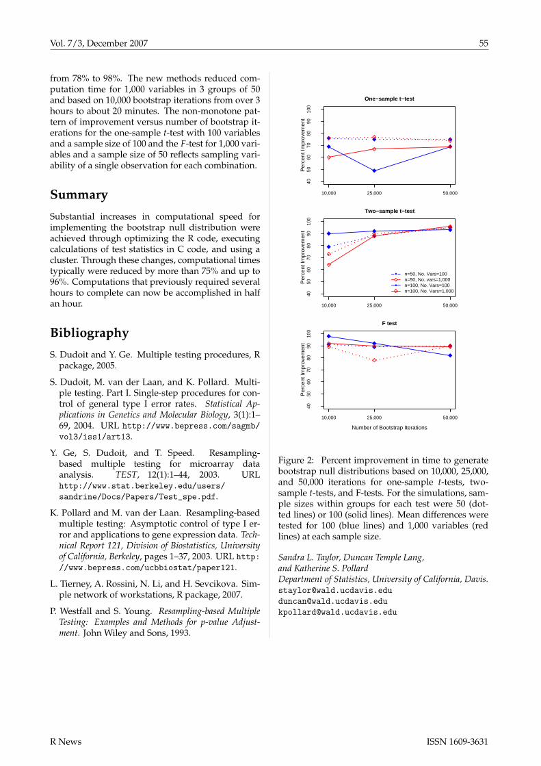
Vol. 7/3, December 2007 55
from 78% to 98%. The new methods reduced com-putation time for 1,000 variables in 3 groups of 50and based on 10,000 bootstrap iterations from over 3hours to about 20 minutes. The non-monotone pat-tern of improvement versus number of bootstrap it-erations for the one-sample t-test with 100 variablesand a sample size of 100 and the F-test for 1,000 vari-ables and a sample size of 50 reflects sampling vari-ability of a single observation for each combination.
Summary
Substantial increases in computational speed forimplementing the bootstrap null distribution wereachieved through optimizing the R code, executingcalculations of test statistics in C code, and using acluster. Through these changes, computational timestypically were reduced by more than 75% and up to96%. Computations that previously required severalhours to complete can now be accomplished in halfan hour.
Bibliography
S. Dudoit and Y. Ge. Multiple testing procedures, Rpackage, 2005.
S. Dudoit, M. van der Laan, and K. Pollard. Multi-ple testing. Part I. Single-step procedures for con-trol of general type I error rates. Statistical Ap-plications in Genetics and Molecular Biology, 3(1):1–69, 2004. URL http://www.bepress.com/sagmb/vol3/iss1/art13.
Y. Ge, S. Dudoit, and T. Speed. Resampling-based multiple testing for microarray dataanalysis. TEST, 12(1):1–44, 2003. URLhttp://www.stat.berkeley.edu/users/sandrine/Docs/Papers/Test_spe.pdf.
K. Pollard and M. van der Laan. Resampling-basedmultiple testing: Asymptotic control of type I er-ror and applications to gene expression data. Tech-nical Report 121, Division of Biostatistics, Universityof California, Berkeley, pages 1–37, 2003. URL http://www.bepress.com/ucbbiostat/paper121.
L. Tierney, A. Rossini, N. Li, and H. Sevcikova. Sim-ple network of workstations, R package, 2007.
P. Westfall and S. Young. Resampling-based MultipleTesting: Examples and Methods for p-value Adjust-ment. John Wiley and Sons, 1993.
4050
6070
8090
100
10,000 25,000 50,000
One−sample t−test
Per
cent
Impr
ovem
ent
4050
6070
8090
100
10,000 25,000 50,000
Two−sample t−test
Per
cent
Impr
ovem
ent
n=50, No. Vars=100n=50, No. vars=1,000n=100, No. Vars=100n=100, No. Vars=1,000
4050
6070
8090
100
10,000 25,000 50,000
F test
Per
cent
Impr
ovem
ent
Number of Bootstrap Iterations
Figure 2: Percent improvement in time to generatebootstrap null distributions based on 10,000, 25,000,and 50,000 iterations for one-sample t-tests, two-sample t-tests, and F-tests. For the simulations, sam-ple sizes within groups for each test were 50 (dot-ted lines) or 100 (solid lines). Mean differences weretested for 100 (blue lines) and 1,000 variables (redlines) at each sample size.
Sandra L. Taylor, Duncan Temple Lang,and Katherine S. PollardDepartment of Statistics, University of California, [email protected]@[email protected]
R News ISSN 1609-3631

Vol. 7/3, December 2007 56
Changes in R 2.6.1by the R Core Team
New features
• The data.frame and factor methods for [[now support the exact argument introduced in2.6.0.
• plot.lm() gains a new argument cex.captionto allow the size of the captions to be con-trolled.
• A series of changes make the CHARSXP cacheintroduced in 2.6.0 faster (and in some casesmany times faster) in sessions with a largenumber (e.g., a million) of unique characterstrings, and also if there are many emptystrings.
• embedFonts(), bitmap() and dev2bitmap()explicitly turn off auto-rotation in Ghostscriptwhen generating PDF.
• The canonical architecture is no longer checkedwhen loading packages using a non-emptysub-architecture, since it is possible to (e.g.)build packages for i386-pc-linux-gnu on boththat architecture and on x86_64-unknown-linux-gnu.
• Deparsing will (if option warnIncomplete isset) warn on strings longer than the parser limit(8192 bytes).
• url() now uses the UserAgent headerin http transactions in the same way asdownload.file() (making use of option"HTTPUserAgent").
Bug fixes
• iconv() is again able to translate characterstrings with embedded nuls (such as those inUCS-2).
• new.packages() and update.packages()failed when called on an empty library,since old.packages() threw an error.old.packages() now returns NULL (as docu-mented) in that case.
• Builds on Mac OS X 10.4 or higher now allocateenough space in the binary headers to relocatedependent libraries into the framework.
• R CMD build now computes the exclusion liston the copy it makes: this avoids problemsif the original sources contain symbolic links
(which are resolved in the copy). Thanks toMichael Lawrence for diagnosis and patch.
• object.size() had slightly too low a size forobjects of type "S4".
• symbol() in plotmath expressions was only ac-cepting valid character strings, which made itimpossible to specify symbols such as aleph(obtained by symbol("300")) in a UTF-8 locale.
• An event handling issue caused autorepeatfunctions to misbehave with tcltk (notablyscrollbars).
• plot(sin, -5, 5) gives ylab "sin(x)" again,where it resulted in "x(x)" in 2.6.0. Further,plot(sin) again plots from [0,1] also in caseswhere a previously used coordinate system dif-fers.
• curve() with unspecified from, to and xlimnow reuses the previous x limits, and notslightly larger ones.
• It was intended that R code filenames in pack-ages should start with an ASCII letter or dig-its (and R CMD INSTALL uses that), but thetest used in R CMD build ([A-Za-z0-9]) waslocale-specific (and excluded t to y in Estonian,for example). (PR#10351)
• R CMD build could misbehave when facedwith files with CRLF line endings and no lineending on the final line of the file, removing thelast byte of the file.
• DF[i, j] failed in 2.6.0 if j was a logical vectorselecting a single column.
• Unix x11() would fail if a valid display wasspecified but DISPLAY was unset. (PR#10379)
• postscript() was not always ignoring.Postscript.Options in the workspace(where it should not have occurred).
• help.search() would give an error if it founda badly installed package, even if package wasnot specified.
• tclServiceMode() (package tcltk) now worksunder Unix-alikes. (Although documented, itused only to work under Windows.)
• As Mac OS X 10.5.0 comes with incompati-ble /bin/sh shell, we force SHELL=/bin/bash(which is ok) in that case. [Only for 2.6.x: an-other solution is used in 2.7.0.]
• Deliberately using malformed source attributesno longer causes deparsing/printing of func-tions to crash R. (PR#10437)
R News ISSN 1609-3631

Vol. 7/3, December 2007 57
• R CMD check and R CMD INSTALL now workwith (some) directory names containingspaces.
• choose(n, k) gave incorrect values for nega-tive n and small k.
• plot.ts(x,y) could use wrong default labels;fixed thanks to Antonio Fabio di Narzo.
• reshape() got column names out of sync withcontents in some cases; found by Antonio FabioDi Narzo.
• ar(x) for short x (i.e., length ≤ 10) couldfail because the default order.max was ≥length(x) which is non-sensical.
• Keyboard events in getGraphicsEvent()could cause stack imbalance errors (PR#10453)
Changes on CRANby Kurt Hornik
New contributed packages
BARD Better Automated ReDistricting and heuris-tic exploration of redistricter revealed prefer-ence. By Micah Altman.
CellularAutomaton An object-oriented implemen-tation of one-dimensional cellular automata.Supports many of the features offered byMathematica, including elementary rules, user-defined rules, radii, user-defined seeding, andplotting. By John Hughes.
ComPairWise Compare phylogenetic or populationgenetic data alignments. By Trina E. Roberts.
EDR Estimation of the effective dimension reduc-tion (EDR) space in multi-index regressionmodels. By Joerg Polzehl.
FGN Fractional Gaussian Noise (FGN) model fit-ting, including MLEs for the H parameter andregression with FGN errors, and simulation ofFGN. By A. I. McLeod.
FKBL Fuzzy Knowledge Base Learning, an R/C im-plementation of a fuzzy inference engine sup-porting several inference methods. By AlvaroGonzalez Alvarez.
FieldSim Routines to simulate random fields.By Alexandre Brouste and Sophie Lambert-Lacroix.
GLDEX Fitting single and mixture of GeneralizedLambda Distributions (RS and FMKL) usingDiscretized and Maximum Likelihood meth-ods. The fitting algorithms considered havetwo major objectives. One is to provide asmoothing device to fit distributions to datausing the weight and unweighted discretizedapproach based on the bin width of the his-togram. The other is to provide a definitive fit
to the data set using the maximum likelihoodestimation. Diagnostics on goodness of fit canbe done via QQ-plots, KS-resample tests andcomparing mean, variance, skewness and kur-tosis of the data with the fitted distribution. BySteve Su.
GillespieSSA Gillespie’s Stochastic Simulation Al-gorithm (SSA). Provides a simple to use, in-tuitive, and extensible interface to severalstochastic simulation algorithms for generat-ing simulated trajectories of finite populationcontinuous-time models. Currently it imple-ments Gillespie’s exact stochastic simulationalgorithm (Direct method) and several ap-proximate methods (Explicit tau-leap, Bino-mial tau-leap, and Optimized tau-leap). Alsocontains a library of template models thatcan be run as demo models and can eas-ily be customized and extended. Currentlythe following models are included: decaying-dimerization reaction set, linear chain sys-tem, logistic growth model, Lotka predator-prey model, Rosenzweig-MacArthur predator-prey model, Kermack-McKendrick SIR model,and a meta-population SIRS model. By MarioPineda-Krch.
HardyWeinberg Exploration of bi-allelic markerdata. Focuses on the graphical representationof the results of tests for Hardy-Weinberg equi-librium in a ternary plot. Routines for severaltests for Hardy-Weinberg equilibrium are in-cluded. By Jan Graffelman.
HiddenMarkov Hidden Markov Models. Containsfunctions for the analysis of Discrete TimeHidden Markov Models, Markov ModulatedGLMs and the Markov Modulated Poisson Pro-cess. Includes functions for simulation, param-eter estimation, and the Viterbi algorithm. Thealgorithms are based of those of Walter Zuc-chini. By David Harte.
JADE JADE and ICA performance criteria. The
R News ISSN 1609-3631

Vol. 7/3, December 2007 58
package ports J.-F. Cardoso’s JADE algorithmas well as his function for joint diagonaliza-tion. There are also several criteria for perfor-mance evaluation of ICA algorithms. By KlausNordhausen, Jean-Francois Cardoso, HannuOja, and Esa Ollila.
JudgeIt Calculates bias, responsiveness, and othercharacteristics of two-party electoral systems,with district-level electoral and other data. ByAndrew Gelman, Gary King, and Andrew C.Thomas.
NestedCohort Estimate hazard ratios, standardizedsurvival and attributable risks for cohorts withmissing covariates, for Cox models or Kaplan-Meier. By Hormuzd A. Katki.
ProfessR Grades setting and exam maker. Programsto determine student grades and create exam-inations from question banks. Programs willcreate numerous multiple choice exams, ran-domly shuffled, for different versions of samequestion list. By Jonathan M. Lees.
RFOC Graphics for statistics on a sphere, as ap-plied to geological fault data, crystallogra-phy, earthquake focal mechanisms, radia-tion patterns, ternary plots and geographi-cal/geological maps. By Jonathan M. Lees.
RHmm Discrete, univariate or multivariate Gaus-sian, mixture of univariate or multivariateGaussian HMM functions for simulation andestimation. By Ollivier Taramasco.
RPMG R Poor Man’s Gui: create interactive R anal-ysis sessions. By Jonathan M. Lees.
RPyGeo ArcGIS Geoprocessing in R via Python.Provides access to (virtually any) ArcGIS Geo-processing tool from within R by runningPython geoprocessing scripts without writingPython code or touching ArcGIS. Requires Ar-cGIS ≥ 9.2, a suitable version of Python (cur-rently 2.4), and Windows. By Alexander Bren-ning.
RSAGA SAGA Geoprocessing and Terrain Analysisin R. Provides access to geocomputing and ter-rain analysis functions of SAGA (http://www.saga-gis.org/) from within R by running thecommand line version of SAGA. In addition,several R functions for handling and manip-ulating ASCII grids are provided, including aflexible framework for applying local or focalfunctions to grids. By Alexander Brenning.
RcmdrPlugin.FactoMineR Rcmdr plugin for pack-age FactoMineR. By Francois Husson, JulieJosse, and Sebastien Le.
Rsundials SUite of Nonlinear DIfferential ALge-braic equations Solvers in R. Provides an inter-face for the package of nonlinear differential al-gebraic equation solvers that comprise SUNDI-ALS. ODEs are expressed as R functions or ascompiled code. By Selwyn-Lloyd McPherson.
Rvelslant Code for interactively analyzing down-hole seismic data and interpreting layered ve-locity models of constant velocity layers ac-counting for refractions across layer bound-aries. Original method by Dave Boore, R portand some additions by Eric M. Thompson.
SASxport Functions for reading, listing the contentsof, and writing SAS XPORT format files. Thefunctions support reading and writing of eitherindividual data frames or sets of data frames.Further, a mechanism has been provided forcustomizing how variables of different datatypes are stored. By Gregory R. Warnes.
SoDA Utilities and examples from the book “Soft-ware for Data Analysis: Programming with R”.By John M Chambers.
StatDA Offers different possibilities to make statis-tical analysis for environmental data. By PeterFilzmoser and Barbara Steiger.
TSMySQL Time Series Database Interface exten-sions for MySQL. By Paul Gilbert.
TSSQLite Time Series Database Interface extensionsfor SQLite. By Paul Gilbert.
TSdbi Time Series Database Interface. By PaulGilbert.
TSpadi TSdbi Interface to PADI Time Series Server(for e.g. Fame). Provides methods for genericsin the TSdbi package to connect through a pro-tocol for application database interface (PADI)to a time series database (e.g., Fame). By PaulGilbert.
TTR Functions and data to construct Technical Trad-ing Rules. By Josh Ulrich.
animation Various functions for animations instatistics, covering many areas such as prob-ability theory, mathematical statistics, multi-variate statistics, nonparamatric statistics, sam-pling survey, linear models, time series, com-putational statistics, data mining and machinelearning. These functions might be of help inteaching statistics and data analysis. By YihuiXie.
bnlearn Bayesian network structure learning viaconstraint-based (also known as “conditionalindependence”) algorithms. This package im-plements the Grow-Shrink (GS) algorithm, the
R News ISSN 1609-3631
Vol. 7/3, December 2007 59
Incremental Association (IAMB) algorithm, theInterleaved-IAMB (Inter-IAMB) algorithm andthe Fast-IAMB (Fast-IAMB) algorithm for bothdiscrete and Gaussian networks. Simulationand some score functions are implemented fordiscrete networks. By Marco Scutari.
bs A collection of utilities for the Birnbaum-Saunders distribution (BSD). By Víctor Leiva,Hugo Hernández, and Marco Riquelme.
cacher Tools for caching statistical analyses in key-value databases which can subsequently bedistributed over the web. By Roger D. Peng.
calib Statistical tool for calibration of plate basedbioassays. By Dan Samarov and Perry Haa-land.
caret Classification And REgression Training: func-tions for training and plotting classification andregression models. By Max Kuhn, Jed Wing,Steve Weston, and Andre Williams.
caretLSF Classification And REgression TrainingLSF style. By Max Kuhn.
caretNWS Classification And REgression Trainingin parallel Using NetworkSpaces. By MaxKuhn and Steve Weston.
cggd Continuous Generalized Gradient Descent. Ef-ficient procedures for fitting an entire regres-sion sequences with different model types. ByCun-Hui Zhang and Ofer Melnik.
demogR Construction and analysis of matrix popu-lation models in R. By James Holland Jones.
dice Calculate probabilities of various dice-rollingevents. By Dylan Arena.
dtw Implementation of Dynamic Time Warp (DTW)and its generalizations. DTW finds the optimalmapping (local time stretch) between a givenquery into a given template time series. Im-plements symmetric, asymmetric, and customstep patterns with weights. Supports window-ing (none, Itakura, Sakoe-Chiba, custom). Out-puts minimum cumulative distance, warpingpaths, etc. By Toni Giorgino, with contribu-tions from Paolo Tormene.
ecespa Some wrappers, functions and data setsfor for spatial point pattern analysis, used inthe book “Introduccion al Analisis Espacialde Datos en Ecologia y Ciencias Ambientales:Metodos y Aplicaciones”. By Marcelino dela Cruz Rot, with contributions of Philip M.Dixon.
fAsianOptions Rmetrics: EBM and Asian optionvaluation. By Diethelm Wuertz and many oth-ers.
fAssets Rmetrics: Assets selection and modeling.By Diethelm Wuertz and many others.
fBonds Rmetrics: Bonds and interest rate models.By Diethelm Wuertz and many others.
fExoticOptions Rmetrics: Exotic option valuation.By Diethelm Wuertz and many others.
fGarch Rmetrics: Autoregressive conditional het-eroskedastic modeling. By Diethelm Wuertzand many others.
fImport Rmetrics: Economic and financial data im-port. By Diethelm Wuertz and many others.
fNonlinear Rmetrics: Nonlinear and chaotic timeseries modeling. By Diethelm Wuertz andmany others.
fRegression Rmetrics: Regression based decisionand prediction. By Diethelm Wuertz and manyothers.
fTrading Rmetrics: Technical trading analysis. ByDiethelm Wuertz and many others.
fUnitRoots Rmetrics: Trends and unit roots. By Di-ethelm Wuertz and many others.
fUtilities Rmetrics utilities. By Diethelm Wuertzand many others.
ff Flat file database designed for large vectors andmulti-dimensional arrays. By Daniel Adler,Oleg Nenadic, Walter Zucchini, and ChristianGlaeser.
fuzzyFDR Exact calculation of fuzzy decision rulesfor multiple testing. Choose to control FDR(false discovery rate) using the Benjamini andHochberg method, or FWER (family wise er-ror rate) using the Bonferroni method. By AlexLewin.
gamlss.cens An add on package to GAMLSSfor fitting interval response variables us-ing gamlss.family distributions. By MikisStasinopoulos, Bob Rigby, and Nicoleta Mor-tan.
glasso Graphical lasso. By Jerome Friedman and R.Tibshirani.
hbim Hill/Bliss Independence Model for combina-tion vaccines. Calculate expected relative riskand proportion protected assuming normallydistributed log10 transformed antibody dosefor several component vaccine. Uses Hill mod-els for each component which are combinedunder Bliss independence. By M. P. Fay.
hints Gives hints on what functions you might wantto apply to an object you have created. ByHadley Wickham and Sanford Weisberg.
R News ISSN 1609-3631

Vol. 7/3, December 2007 60
ig A collection of utilities for robust and classicalversions of the inverse Gaussian distributionknown as inverse Gaussian type distribution(IGTD). By Víctor Leiva, Hugo Hernández, andAntonio Sanhueza.
lga Tools for linear grouping analysis (LGA). ByJustin Harrington.
logilasso Analysis of sparse contingency tables withpenalization approaches. By Corinne Dahin-den.
ltsa Linear time series analysis. Methods are givenfor loglikelihood computation, forecasting andsimulation. By A. I. McLeod, Hao Yu, and Zi-novi Krougly.
matrixcalc A collection of functions to support ma-trix differential calculus as presented in Mag-nus and Neudecker (1999) “Matrix Differen-tial Calculus with Applications in Statistics andEconometrics”, Second Edition, John Wiley,New York. Some of the functions are compa-rable to APL and J functions which are usefulfor actuarial models and calculations. By Fred-erick Novomestky.
mefa Faunistic count data handling and report-ing. The name “mefa” stands for the term“metafaunistics” indicating that handling ofbasic data is only the first, but the most criti-cal and sometimes most time consuming partof data analysis. It contains functions to cre-ate and manage objects combining basic faunis-tic (sample/species/count or crosstabulated)count data and sample/species attribute tables.Segments within the count data and sampleswith zero count can be indicated and used insubsequent operations. Reports can be gener-ated in plain text or LATEX format. By Peter Soly-mos.
mlegp Maximum Likelihood Estimates of GaussianProcesses for univariate and multi-dimensionaloutputs with diagnostic plots and sensitivityanalysis. By Garrett M. Dancik.
mra Analysis of mark-recapture (capture-recapture)data using individual, time, and individual-time varying covariates. Contains functionsto estimate live-capture Cormack-Jolly-Seberopen population models. By Trent McDonald.
nnls An R interface to the Lawson-Hanson NNLSalgorithm for non-negative least squares thatsolves the least squares problem Ax = b withthe constraint x >= 0. By Katharine M.Mullen.
nonbinROC ROC-type analysis for non-binary goldstandards. Estimate and compare the accura-cies of diagnostic tests in situations where the
gold standard is continuous, ordinal or nomi-nal. By Paul Nguyen.
paleoTSalt Modeling evolution in paleontologicaltime-series (alternate parametrization). Facili-tates the analysis of paleontological sequencesof trait values from an evolving lineage. Func-tions are provided to fit, using maximum likeli-hood, evolutionary models including unbiasedrandom walks, directional evolution, stasis andOrnstein-Uhlenbeck (OU) models. Performsmany of the same functions as package pale-oTS, but does so using a different parametriza-tion of the evolutionary models. By Gene Hunt.
playwith A GUI for interactive plots using GTK+.Tries to work out the structure of a plot, in or-der to interact with it. The built-in features in-clude: navigating the data space, identifyingdata points, editing and annotating the plot,and saving to a file. New tools can be defined.Note: the interaction features do not work withmultiple-plot layouts. Based on RGtk2, andso requires the GTK+ libraries, and still verymuch under development.
ppls Linear and nonlinear regression methodsbased on Partial Least Squares and Penaliza-tion Techniques. By Nicole Kraemer and Anne-Laure Boulesteix.
predbayescor Classification rule based on naiveBayes models with feature selection bias cor-rected. By Longhai Li.
predmixcor Classification rule based on Bayesianmixture models with feature selection bias cor-rected. By Longhai Li.
pseudo Various functions for computing pseudo-observations for censored data regression. ByMette Gerster and Maja Pohar Perme.
ramps Bayesian geostatistical modeling of Gaus-sian processes using a reparametrized andmarginalized posterior sampling (RAMPS) al-gorithm designed to lower autocorrelation inMCMC samples. Package performance istuned for large spatial datasets. By Brian J.Smith, Jun Yan, and Mary Kathryn Cowles.
realized Realized Variance Toolkit. By Scott Pay-seur.
regsubseq Detect and test regular sequences andsubsequences. For a sequence of event occur-rence times, we are interested in finding subse-quences in it that are too “regular” (in the senseof being significantly different from a homoge-neous Poisson process). By Yanming Di.
sendplot A tool for sending interactive plots. ByDaniel P Gaile, Lori A. Shepherd, Lara Suche-ston, Andrew Bruno, and Kenneth F. Manly.
R News ISSN 1609-3631

Vol. 7/3, December 2007 61
sets Data structures and basic operations for ordi-nary sets, and generalizations such as fuzzysets, multisets, and fuzzy multisets. By DavidMeyer and Kurt Hornik.
surv2sample Two-sample tests for survival analy-sis. Provides tests for comparing two sur-vival distributions, testing equality of two cu-mulative incidence functions under competingrisks and checking goodness of fit of propor-tional rate models (proportional hazards, pro-portional odds) for two samples. By DavidKraus.
zoeppritz Zoeppritz equations: calculate and plotscattering matrix coefficients for plane waves
at interface. By Jonathan M. Lees.
Other changes
• Packages FLCore, FLEDA, FortranCallsR,GammaTest, InfNet, RcppTemplate, edci,limma, rcompletion, and roblm were movedto the Archive.
• Packages StoppingRules and pwt were re-moved from CRAN.
Kurt HornikWirtschaftsuniversität Wien, [email protected]
R News ISSN 1609-3631

Vol. 7/3, December 2007 62
Editor-in-Chief:Torsten HothornInstitut für StatistikLudwigs–Maximilians–Universität MünchenLudwigstraße 33, D-80539 MünchenGermany
Editorial Board:John Fox and Vincent Carey.
Editor Programmer’s Niche:Bill Venables
Editor Help Desk:Uwe Ligges
Email of editors and editorial board:firstname.lastname @R-project.org
R News is a publication of the R Foundation for Sta-tistical Computing. Communications regarding thispublication should be addressed to the editors. Allarticles are copyrighted by the respective authors.Please send submissions to regular columns to therespective column editor and all other submissionsto the editor-in-chief or another member of the edi-torial board. More detailed submission instructionscan be found on the R homepage.
R Project Homepage:http://www.R-project.org/
This newsletter is available online athttp://CRAN.R-project.org/doc/Rnews/
R News ISSN 1609-3631