AL/HR-TP-19W3-0034 AD-A273 880

AIRMAN APPUCANT PREDICTION SYSTEM (AAPS):

THEORY AND RESULTS

ARM Bice M. Stone DTICS Kathym L Tumrer S

8301 Boadway, Suite 215 . DEC 16 1993

R Antonio, TX 79= E0EN Shores K. Engquist, Major, USAF

G aLarry T. LooperJamlie K. Viera, Second Ueutenant, USAF

HUMAN RESOURCES DIRECTORATEMANPOWER AND PERSONNEL DIVISION

L 7909 Undbergh Drive

A Brooks Air Force Base, TX 78235-5352

B0 November 1993

R Final Technical Paper for Period February 1991 - may 1992

T0 Approved for public release; distribuion is unlimited.

RY

93-30404

93 12 15004

AIR FORCE MATERIEL COMMANDBROOKS AIR FORCE BASE, TEXAS ,_I

BestAvailable

Copy

NOTICES

This technical paper Is published as received and has not been edited by thetechnical editn staff of the Anmstrong Laboratory.

When Governrnt drawings, specifications, or other data we used ior any purposeother than in connection with a defnlte Govemment-related Wocurment, the UnitedStates Garnmert incurs no reponsbilly or any obigation whatsoever. The fact thatthe Government may have formulated or in any way supplied the said drawings,specifications, or other data, is not to be regarded by implication, or otherwise in anymanner construed, as licensing the holder, or any other person or corporatm; or asconveying any rights or pemdssion to manufacture, use, or sell any patented inventionthat may in any way be related thereto.

The Office of Public Affairs has reviewed this paper, and it is releasable to theNational Technical Information Service, where it will be available to the general public,incd foreign nationals

This paper has been reviewed and is approved for publcation.

LARRY T. LOOPER WILUAM E. ALLEY, TechnicalProiect Scientist Manpower and Personnl Reseach

WILLARD BEAVERS, Lt Col, USAFChief, Mapoe ad Personnel Research Division

REPORT DOCUMENTATION PAGE OM .00

Novembr 1 W3Final -February 1991 - May 19924. TITLE AND SUBTITLE &. FUNDING NUMBERSAirman Applicanit Prediction System (AAP$): Theory and Results C - F41 689-88D-02l

PE - 62205F*PR - 7719

6.AUTHOR(S) rA - 20Brice M. Stone Sheres K Engquist WU- 20Ksthryn L Turner Larry T. Looper

Janelle K Viera

7. PERFORMIG ORGANIZATION NAME(S) AND ADOMESS(S) L. PERFORMING ORGANI7ATIONMetrics, Incorporated REPORT NUMBER8301 Broadw!& Suite 215

San ntoio, 78209

6.11 ORIOGIMITORING AGENCY NAMES(S) AND ADDRESS(ES) RE. PONSRTNUMBE OR N AECArmstrong Laboratory (AFMC)REOTNMRHuman Resources Directorate AL/HR-TP-1993-0034Manower and Personnel Research Division

79 ULndbergh DriveBrooks Air Force Base, TX_78235-5352 ___________

11. SUPPLEMENTARY NOTES

Armstrong Laboratory Technical Monitor: Larry T. Looper, (210) 536-3648

121. DISTRIBUTIOWIAVAILABIUITY STATEMENT 12b. DISTRIBUTION CODE

Approved for public release; distribution is unlimited.

13.ABSTRACT (Maxtum 200 words)

The objective of this research effort was to design a model(s) to estimate the impact of key demographicvariable on indiviual and group accession behavior. This would provide personnel managers the ability toproject the quality mix of future accessions and track the impact of this quality mix on enlisted retention behavioras these accessions advance through a militar career. Six demographic groups were analyzed: males, females,Caucasians, Blacks, others, and all. Within each demographic group, four aptitude groups were studied: ArmedForces Qualifying Test (AFOT) Categories I's, 11's, lila's, and Itlb's. The results of the modeling and estimationeffort were Implemented into the Airman Applicant Prediction System (AAPS) to predict the number of applicantsfrom selected demographic/aptitude groups. The estimated equations were used to predict the proportion of aMilitary Availabl (MA) population which would be interested In applying to the Air Force (by AFOT Category).MAPS proceeds through a series of steps to arrive at population numbers for Interested Qualified Military Available(QQMA). IQMA can then be disaggregated through the AAPS software to determine from the 1OMA populationwho would potentially meet mechanical, administrative, general, and eiectronic (MAGE) minimum Armed ServicesVocationtal Aptitude Battery (ASVAB) composite score requirements.

14.SUBJEC TERMS 15.NUMBER 01'PAGESApplicant prediction Enlisted force projection model 4Demographic applicant breakout Military available 16. PRICE CODE

17.SEC~fY CASIFICATION 115. SECURITY CLASSIFICATION 119. SECURITY CLASSIFICATION 20. LIMITATION Of ABSTRACTIOF REOTOF PAGEIOAFA~ndUncl~wassIfie clasiie aSfe UL_______

HNS 75UdO,104NO f4IOOL-I=0-102

TABLE OF CONTENTS

SUM M ARY .............................................. 1

INTRODUCTION 1........................................... I

DEMOGRAPHIC ACCESSION LITERATURE ......................... 2

DATA DESCRIPTION ........................................ 4

Application Rate ....................................... 4Wage and Unemployment Data ................................... 5Recruiting Data ........................................ 5Binary Variables . ...................................... 7

ESTIMATION OF THE DEMOGRAPHIC MODELS ....................... 8

M ales .............................................. 8Females ............................................. 10Caucasians ........................................... 12Blacks .............................................. 13Others .............................................. 15All ................................................ 16Elasticities ........................................... 17Explanatory Credibility of Equationss ........................... 19Summary of Estimation Results ................................ 21

IMPLEMENTATION OF THE DEMOGRAPHIC MODELS INTO AAPS ........ 22

M ilitary Available ...................................... 23Interested Military Available ................................. 26Interested Qualified Military Available ............................ 28The MAGE Distribution of the IQMA Population ..................... 30

AIRMAN APPLICANT PREDICTION SYSTEM SOFTWARE ................ 30

Census Constraints ........................................ 30Economic Constraints .................................... 31Availability Constraints ..................................... 31Forecasting Predictions ..................................... 31

CONCLUSIONS ............................................ 32

iii

.• ' ii? ... .......

REFERENCES ............................................. 34

APPENDIX ................................................ 36

LIST OF TABLES

Table Page

1. Relative Military to Civilian Wage Elasticities ......................... 32. Variable Definitions ........................................ 43. Means (standard deviations) of Explanatory Variables ..................... 64. Means (standard deviations) of Other Variables .......................... 75. Coefficients for Males by AFQT Categories ............................ 96. Coefficients for Females by AFQT Categories ........................ 117. Coefficients for Caucasians by AFQT Categories ........................ 138. Coefficients for Blacks by AFQT Categories .......................... 149. Coefficients for Others by AFQT Categories .......................... 1510. Coefficients for All by AFQT Categories ............................ 1611. Relative Wage Elasticities for Demographic

and Aptitude Groups ...................................... 1812. Unemployment Elasticities for Demographic

and Aptitude Groups ...................................... 1813. Recruiter Elasticities for Demographic

and Aptitude Groups ...................................... 1914. R2s for Equations ......................................... 2015. Sample Means for Application Numbers ........................... 2016. In-Sample and Out-of-Sample RMSEs ............................... 21

iv

PREFACE

This research and development effort was conducted as task order 49 under Contract F41689-88-D-0251 (SBA 68822004) by Metrica, Inc. for the Manpower and Personnel Research Divisionof the Armstrong Laboratory, Human Resources Directorate (AL/HR). The purpose of thiseffort was to design a model to estimate the impact of key demographic variables on individualand group accession behavior which directly impact the retention of enlisted personnel in the AirForce.

The authors wish to thank Mr Vincent Wiggins and Mrs LeAnn Coleman for their valuabletechnical contributions to this effort. In addition, the authors would like to express appreciationto Ms Barbara Randall (computer programmer), Mr Kevin Borden (computer programmer), andMr Darryl Hand (computer programmer).

Accesion ForNTIS CRA&IDTIC TABUnannounced 0Justification

By -- ..........By ............. ...... .. . .

Dist, ibution I

Availability Codes

I Avail and / orDist Special

V

AIRMAN APPLICANT PREDICTION SYSTEM (AAPS):

THEORY AND RESULTS

S• SUMMARY

The objective of this research effort was to design a model(s) to estimate the impact of keyS" demographic variables on individual and group accession behavior. The demographic factors of

the supply model were gender, race, and geographic location (state). In addition, the analysisinvestigated the propensity of Armed Forces Qualifying Test (AFQT) categories 1, 11, MIIa, andmb to apply for Air Force service.

The analysis used pooled time series, cross-sectional (state level) data extracted from thehistorical Military Entrance Processing Stations (MEPS) data combined with population data fromthe Bureau of the Census; earnings and employment data from the Bureau of Labor Statistics(BLS); and data on production recruiters, numbers in the Delayed Entry Program (DEP), andrecruiting goals from Air Force Recruiting Service. Twenty equations were estimated, one foreach demographic and aptitude group. The equations were estimated using monthly data fromJanuary 1983 to December 1989. The out-of-sample credibility of the esti' hed equations wasvalidated using data from January 1990 to December 1990.

The results of the modeling effort were implemented into the Airman Applicant PredictionSystem (AAPS), a user-friendly, menu-driven, PC software package which predicts the flow ofselected demographic groups into the Air Force from an available population. The estimatedequations can be used to predict the proportion of a Military Available population which will beinterested in applying to the Air Force (by AFQT category). AAPS proceeds through a seriesof steps to arrive at population numbers for Interested Qualified Military Available (IQMA).IQMA can then be disaggregated through the AAPS software to determine the number of theIQMA population who would potentially meet mechanical, administrative, general, and electronic(MAGE) minimum Armed Forces Vocational Aptitude Battery (ASVAB) composite scorerequirements.

INTRODUCTION

The Air Force accesses, trains, and separates thousands of young men and women each year.Recruiting goals are established based upon the projections for retention and force levelrequirements. The difficulty of reaching Air Force recruiting goals is reflected in changes in therecruiting budget, short-term recruiting shortfalls, and fluctuations in the overall quality ofrecruits. The need to anticipate problems in the accession and retention of quality personnel andthe attainment of recruiting goals, particularly the level of effort required (e.g., number ofproduction recruiters), is important to a cost-effective and efficient allocation of resources torecruiting programs. In addition, anticipating fluctuations in overall accession and retentionquality allows personnel managers to adjust personnel flows into career fields internally throughprograms such as cross-training. Such internal adjustments minimize the short-term and long-

! 1

term effect of quality fluctuations on the mission readiness of the total force. Thus, there is greatneed for a model which can address the impact of changing demographics on the accession ofpotential recruits.

Managing and maintaining the enlisted force not only requires projecting future flows ofpersonnel but also projecting the quality level of those future flows which affect the ability of theAir Force to meet short-run and long-run mission readiness. Jobs in the Air Force require arange of talents and capabilities to operate and maintain many of the technologically advancedweapon systems. Given a foreseeable decline in the qualified youth population, models to predictaccession/retention flows of demographic groups are essential to efficient, cost effectivemanagement of Air Force personnel and allocation of recruiting resources.

DEMOGRAPHIC ACCESSION LITERATURE

Past and present research has used time series, cross-sectional, and pooled time series, cross-sectional data to analyze fluctuations in the quality and flow of military personnel (Saving,Battalio, DeVany, Dwyer, and Kagel, 1980; DeVany and Saving, 1982; Daula, Fagan, andSmith, 1982; Saving and Stone, 1983; Curtis, Borack, and Wax, 1987; Hosek and Peterson,1985; Orvis, Gahart, and Hosek, 1989; Stone, Saving, Turner, Looper, and Engquist, 1991).The use of suricy data as a basis for modeling the impact of demographic factors such as race,gender and education level has been limited, though often providing unique opportunities toanalyze intricate questions (Daula, Fagan, and Smith, 1982; Orvis and Gahart, 1985; Orvis andGahart, 1989; House, Saving, and Stone, 1985a; House, Saving, and Stone, 1985b).

One source of demographic and attitudinal data concerning potential accessions is the YouthAttitude Tracking Survey (YATS), performed annually for the Office of the Assistant Secretaryof Defense for Force Management and Personnel. YATS provides information on the likelihoodof future military service, effects of advertising and recruiting, and other characteristics andattitudes of the youth population. Combining the YATS data with Air Force personnel,economic, and personnel policy information can provide a unique opportunity to analyze andestimate conditional probabilities to enlist for various combinations of demographic groups.Additional information can be obtained from these probabilities if they are calculated at levelsof qualitative/demographic disaggregation such as Air Force Qualifying Test (AFQT) mentalcategories, gender, and race (Saving et al., 1980).

Several studies have modeled the flow of AFQT aptitude groups into the military. Twostudies which are particularly important for this analysis are the Cotterman (1986) and Goldbergand Goldberg (1988) studies. In both studies, the model estimation used pooled time series,cross-sectional monthly data, disaggregated to the state level. The Goldbergs analyzed the flowof non-prior service (NPS), male, high school diploma graduates (HSDGs), AFQT mentalcategories I through liMa, IMb, and I through MIb enlistments (signed contracts) across all fourbranches of service. Separate models were estimated for each AFQT category for each service.Goldberg's dependent variable was defined as the number of enlistment contracts signed for each

2

service at time t in state s, divided by the population of male, high school seniors at time t instate s for the time period October 1979 through September 1987. Cotterman (1986) alsoestimated the flow of AFQT mental categories I through lMla, HSDGs by service using pooledtime series, cross-sectional (state level) data. Cotterman's dependent variable was defined asthe number of enlistment contracts signed for each service at time t in state s, divided by thepopulation of 17 to 21 year old males at time t in state s for the time period October 1974through March 1981.

The enlistment rates (dependent variables) analyzed by the Goldbergs and Cotterman weresimilar, differing only in the assumption concerning the population from which the enlistmentswere drawn. The key difference between the two studies was in the estimation method: theGoldbergs used an autoregressive moving average regression method with explanatory variables,estimating each equation separately, while Cotterman selected a generalized least squares systemsmethod, estimating the four service equations simultaneously. As shown in Table 1, the relativemilitary to civilian pay elasticities were similar in range between the Goldbergs' and Cottermanstudies but differed significantly in value by service.

Table 1. Relative Military to Civilian Wage Elasticities

Service [Army Navy Marine Air Force]

Goldberg 1.350 0.540 1.340 0.510

Cotterman 0.523 0.651 1.270 0.613

Dale and Gilroy (1984) also obtained similar relative wage elasticities for the Army flow ofNPS male HSDGs, for AFQT mental categories I through IIla which ranged from 0.9 to 1.7.

In past studies such as Cotterman (1986) and Goldberg and Goidberg (1988), the numberof contracts was used as the numerator of the dependent variable. For this present study, thenumber of applicants was selected as the numerator of the dependent variable, instead ofenlistments (signed contracts) as the Goldbergs and Cotterman had used, for two reasons:(1) the date of application for a prospective recruit is closer to the actual time of the decisionto enlist and, thus, closer to the economic/recruitment environment which precipitated theapplicant's decision to apply and (2) applicant flows are less constrained by recruiting goalsand enlistment standards and, thus, are a better reflection of the effects ofeconomic/recruitment factors on the actual flow of applicants into the MEPS.

3

DATA DESCRITIION

This study used pooled time series, cross-sectional (state level) data to estimate supplyequations for the rate of flow of Air Force applicants by demographic groups (gender and race)and aptitude groups (AFQT mental category). The applicant flows were defined as the numberof MEPS applications at time t in state s for demographic group I and AFQT mental categoryk divided by the 17 to 21 year old youth population for state s and with demographic group.Equations were estimated for four aptitude categories (AFQT mental category 1, II, Lila, and11Tb) for each of six demographic groups: males, females, Caucasians, Blacks, others, and all(regardless of gender or race). Each equation was estimated over the January 1983 to December1989 time period. Out-of-sample validation was done for each equation over the January 1990to December 1990 time period. Table 2 contains definitions of the variables used for theestimations, as well as the expected sign of each variable.

Table 2. Variable Definitions

Variable Name Variable Definition Expted Sign

RMEPS MEPS applicants / (17 - 21) population n/a

RECR Number of production recruiters +

UEMP Unemployment rate for 16-24 year olds +

RLWG Relative military to civilian wage +

GLFY Proximity to fiscal year accession goal -

REZO No contracts allowed period -

FIBK Recruits in DEP for next fiscal year -

DDEP Pay longevity change for DEP -

QTR* Quarterly dummy variables undefined

ST* State dummy variables undefined

Application Rate

Data for the calculation of the application rate were obtained from the MEPS files maintainedat Armstrong Laboratory, Human Resources Directorate (Brooks AFB) for the time periodJanuary 1983 through December 1990. The dependent variable was defined as the ratio of thenumber of Air Force applicants arriving at the MEPS monthly by state, by the earliest MEPSapplication date, to the 17 to 21 year old noninstitutionalized population by state with a high

4

school diploma and not in college. The population data were obtained from the Bureau of theCensus.

Records for MEPS applicant! -flen occur more than once in the historical MEPS files asapplicants reapply for entry ir'. the Air Force, retake the ASVAB test or retake the physicalexamination. This analysis made each applicant unique, ignoring duplicates if the individualapplied more than once. The only exception was that an individual who made a subsequentapplication 24 months after the previous application was considered a new applicant.

Wage and Unemployment Data

The relative military to civilian wage (RLWG) was calculated as the ratio of military tocivilian pay over the first four years of the recruit's military service. Civilian wages werecalculated from state specific, private nonagricultural wage data obtained from the Bureau ofLabor Statistics (BLS). Military pay included basic pay, basic allowance for quarters (BAQ),basic allowance for subsistence (BAS), tax allowances, and promotion opportunities over fouryears of active duty.

Monthly unemployment rates, UEMP by state for 16 to 24 year olds by gender and race werealso obtained from the BLS for the January 1983 to December 1990 time period. Two problemsencountered with this data caused a reduction in the number of states for which application ratesfor the Black and other racial groups could be estimated: (1) unemployment rates for Black andother youths were missing in the Bureau of Labor Statistics (BLS) data for 10% or more of thetime periods for many of the states, as well as exhibiting erratic variations due to small laborforce populations numbers in these states, and (2) the number of applications for Blacks andothers within AFQT mental categories from the states (with unemployment problems) was zerofor many of the time periods and small in many of the other time periods. Thus, twenty-fivestates were included for Blacks, while only eight states were included for the other category.

Mean values and standard deviations for RLWG and UEMP are provided in Table 3 for eachdemographic group. Sample size and number of states available for each demographic group arealso provided in Table 3. States available for Blacks included: AL, AR, CA, DC, DE, FL,GA, IL, LA, MA, MD, MI, MO, MS, NJ, NV, NY, NC, OH, OK, PA, SC, TN, TX, and VA.States available for the other category included: AK, CA. HI, MT, NM, NY, OK, and SD.

Recruiting Data

In order to obtain monthly, state level recruiting data, distributions were performed onquarterly snapshots of the Uniform Airman Reports from December 1982 to December 1990.Two fields were used to identify the recruiters: ASSIGNMENT(ASGT)-CURRENT-COUNTRY/STATE and Duty AFSC (Air Force Specialty Code). A distribution on ASGT-CURRENT-COUNTRY/STATE was performed across all records for which the Duty AFSC (5-digit level) was equal to 99500, the code identifying a recruiter. The ASGT-CURRENT-COUNTRY/STATE field provided the number of the recruiters by state, RECR. Total recruiter

5

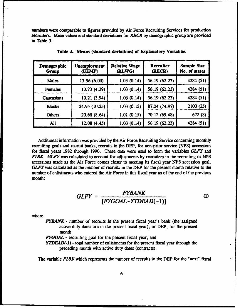
numbers were comparable to figures provided by Air Force Recruiting Services for productionrecruiters. Mean values and standard deviations for RECR by demographic group are providedin Table 3.

Table 3. Means (standard deviations) of Explanatory Variables

Demographic Unemployment Relative Wage Recruiter Sample Size

Group (UEMP) (RLWG) (RECR) No. of states

Males 13.56 (6.00) 1.03 (0.14) 56.19 (62.23) 4284 (51)

Females 10.73 (4.39) 1.03 (0.14) 56.19 (62.23) 4284 (51)

Caucasians 10.21 (3.94) 1.03 (0.14) 56.19 (62.23) 4284 (51)

Blacks 24.95 (10.25) 1.03 (0.15) 87.24 (74.97) 2100 (25)

Others 20.68 (8.64) 1.01 (0.15) 70.12 (69.48) 672 (8)

All 12.08 (4.45) 1.03 (0.14) 56.19 (62.23) 4284 (51)

Additional information was provided by the Air Force Recruiting Service concerning monthlyrecruiting goals and recruit banks, recruits in the DEP, for non-prior service (NPS) accessionsfor fiscal years 1982 through 1990. These data were used to form the variables GLFY andFiBR. GLFY was calculated to account for adjustments by recruiters in the recruiting of NPSaccessions made as the Air Force comes closer to meeting its fiscal year NPS accession goal.GLFY was calculated as the number of recruits in the DEP for the present month relative to thenumber of enlistments who entered the Air Force in this fiscal year as of the end of the previousmonth:

GUITFYBANKGLFY = FYAN 1)[FYGOAL - YTDFAD( -1)]

whereFYBANK - number of recruits in the present fiscal year's bank (the assigned

active duty dates are in the present fiscal year), or DEP, for the presentmonth

FYGOAL - recruiting goal for the present fiscal year, andYTDEAD(-1) - total number of enlistments for the present fiscal year through the

preceding month with active duty dates (contracts).

The variable FlBK which represents the number of recruits in the DEP for the "next" fiscal

6

year was calculated to attempt to capture the effects of recruiters "stockpiling" recruits for thenext fiscal year.

FIBK = TOTEK-FYBANK (2)

where

VTOTK - total number of recruits in the bank for the present month.

Mean values and standard deviations for GLFY and FIBK are provided in Table 4.

Table 4. Means (standard deviations) of Other Variables

Variable Mean (std. dev.)

GLFY 0.59 (0.21)

F1BK 9635.70 (9596.84)

REZO 0.02(0.15)

DDEP 0.65 (0.48)

QTR1 0.25 (0.43)

QTR3 0.25 (C.43)

QTR4 0,25 (0.43)

Binary Variables

REZO is a binary variable included in the estimation to account for the three month timeperiod during November 1989 to January 1990 (REZO = 1). During this time period recruiterswere not permitted to sign contracts with recruits due to the large force drawdowns required tomeet end-of-fiscal-year force level requirements. Another binary variable was included, DDEP.This variable accounts for the change in policy which no longer allowed time in the DEP to counttowards longevity pay. This change occurred in June 1985.

The time period of enlistment is represented as categorical variables (QTR1, QTR3, andQTR4) with QTR2 being a component of the constant term. QTRI represents the first quarterof the fiscal year. These time variables are present in each equation. Table 4 presents the meansand standard deviations for each of these binary variables. Dummy variables are also includedfor each state in the estimation.

7

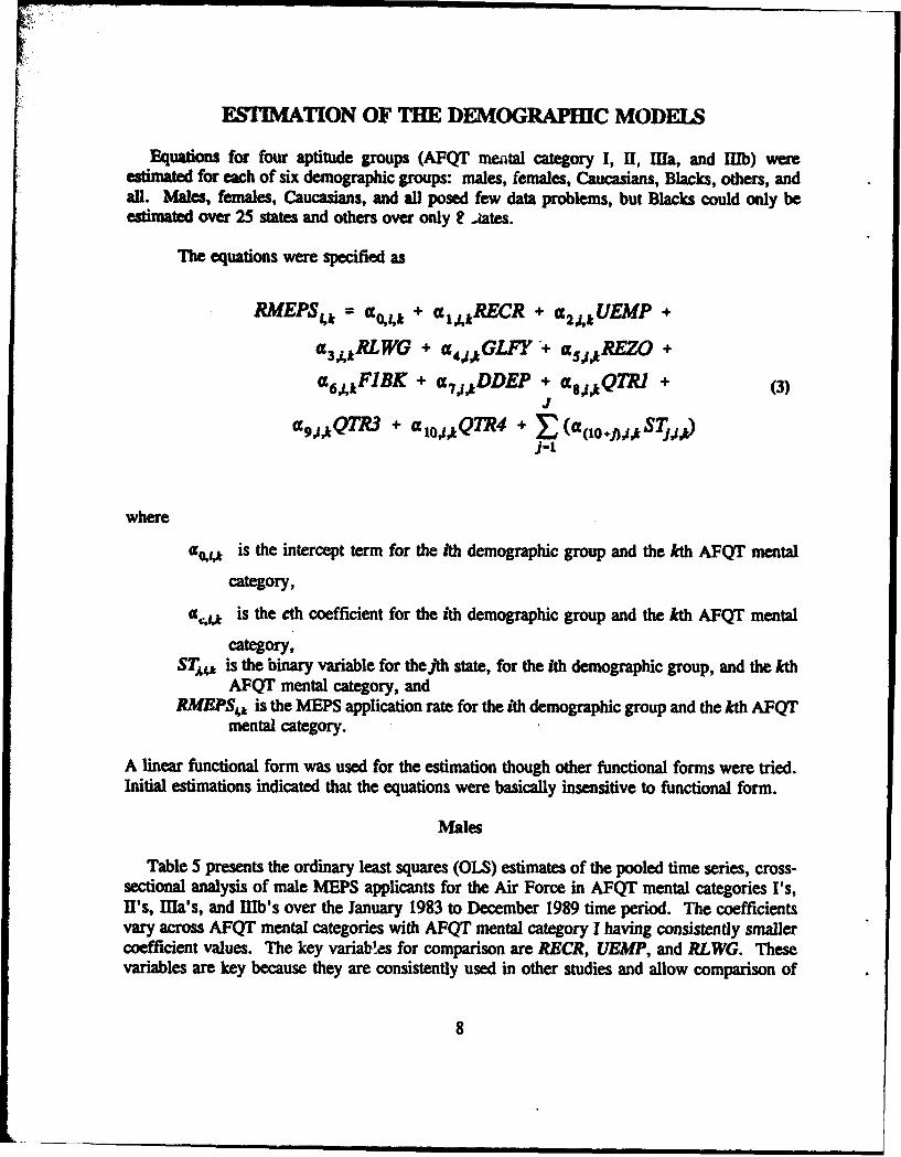
ESTIMATION OF THE DEMOGRAPHIC MODELS

Equations for four aptitude groups (AFQT mental category I, 1, MiTa, and Ilib) wereestimated for each of six demographic groups: males, females, Caucasians, Blacks, others, andall. Males, females, Caucasians, and all posed few data problems, but Blacks could only beestimated over 25 states and others over only P .oates.

The equations were specified as

RMEPS,, = cc 4kt + al,4 kRECR + a 2AUEMP +

a 3AtRLWG + a4J,tGLFY "+ cg•,kRETZO +

t 6 ,4 kF1BK + a 7 J,kDDEP + askQTRJ + (3)

a 9,,,QTR3 + £103,,kQTR4 + EX at j~tSj,J-t

where

606e A is the intercept term for the ith demographic group and the kth AFQT mental

category,

U,,a is the cth coefficient for the ith demographic group and the kth AFQT mental

category,STAIA is the binary variable for thejth state, for the ith demographic group, and the kth

AFQT mental category, andRMEPSt is the MEPS application rate for the ith demographic group and the kth AFQT

mental category.

A linear functional form was used for the estimation though other functional forms were tried.Initial estimations indicated that the equations were basically insensitive to functional form.

Males

Table 5 presents the ordinary least squares (OLS) estimates of the pooled time series, cross-sectional analysis of male MEPS applicants for the Air Force in AFQT mental categories I's,H's, Mia's, and lib's over the January 1983 to December 1989 time period. The coefficientsvary across AFQT mental categories with AFQT mental category I having consistently smallercoefficient values. The key variab'es for comparison are RECR, UEMP, and RLWG. Thesevariables are key because they are consistently used in other studies and allow comparison of

8

coefficients and elasticities across studies, and because with the exception of GLFY and FIBE,Sthes are the only continuous independent variables in the estimated equations. Coefficients forthe state binary variables have been included in the constant. RECR and UEMP werestatistically significant at the 99% level across AFQT mental categories with RLWG statisticallysignificant in 3 of the 4 AFQT mental categories. RLWG was statistically significant at the 98%level of confidence for AFQT mental category I.

Table S. Coefficients for Males by AFQT Categories

AFQ2II AFQUIH AEQLUT AEQLI I

CONS -0.0748 -0.8438 -0.9073 -0.8837RECR 0.0021I" 0.0148" 0.0083" 0.0112"UEMP 0.0013" 0.0140" 0.0076" 0.0078mRLWG 0. 1170 1.2933" 1.0969" 0.9347"GUY 0.0702" 0.3836" 0. 1929" 0.3010"REZO -0.073r7 -0.5354" -0.4074" -0.4613"F1BK 0.0032" 0.0121" 0.0052" 0.0122"DDEP 0.0123" -0.0120 0.0488" 0.0413"QTR1 -0.0003 -0.0565" 0.0130 0.0452*

QTR3 -0.0455" -0.2658" -0.1126" -0. 1517"QTR4 -0.0465" -0. 1274" -0.0191 -0.0886

No. of obs 4284 4284 4284 4284F(60,4223) 14.82 48.78 43.77 57.85w 0.174 0.409 0.383 0.451RMSE (In-sample) 0.108 0.429 0.290 0.339RMSE

(Out-of-sample) 0.118 0.444 0.296 0.383

"p < .01"p < .05

9

The largest effect of RBCR on the flow of MEPS applicants occurred for AFQT mentalcategory H. The coefficient of 0.0148 means that an increase of I recruiter will increase theapplication rate of AFQT mental category II by 0.0148 or approximately 625 additional AFQTmental category H1 applicants (0.0148 times the average male population, 42,248.41 in thousands,over the estimation time period). The largest coefficient for UEMP was also for AFQT mental"category H's, 0.0140. This coefficient value implies that if unemployment declines by 0.5percentage points, then the application rate for AFQT mental category U's will decline by 0.0070or approximately 296 fewer AFQT mental category Ii's will apply to the Air Force.

The largest coefficient for RLWG was for AFQT mental category H's, 1.2933. Thiscoefficient value implies that if the relative military to civilian wage declines by 0.05 points, thenthe application rate for AFQT mental category U's will decline by 0.0647 (1.2933 times 0.05)or approximately 2,732 fewer male AFQT mental category U's will apply to the Air Force. Themean value for RLWG over the estimation time period was 1.0276 with a standard deviation of0.1364. This results in a relative wage elasticity of 1.062. The elasticity is defined as (Becker,1971)

eatity = Coefcient x ( independentvariable mean (4)dependentvariable mean

which means the calculation for the relative wage elasticity for AFQT mental category U's isequal to

10276elasticityRLWo = 1.2933x(t* ) = 1.062 (5)1.2513

The wage elasticities for AFQT mental categories I, Mia, and Mlb are 0.792, 1.504, and 1.146,respectively. These elasticities are similar in range of value to the elasticities reported in TableI (Cotterman, 1986 and Goldberg and Goldberg, 1988).

Females

Table 6 presents the OLS estimates of female MEPS applicants. The coefficients vary acrossAFQT mental categories with AFQT mental category I, once again, having consistently smallercoefficient values. The magnitude of the effects of economic and recruiting factors on thedecision of AFQT mental category I's to join the Air Force relative to the other AFQT mentalcategories is not unexpected. AFQT mental category I's would be expected to have the highestopportunity cost (e.g., more opportunity for employment or other endeavors outside of the AirForce) of the AFQT mental categories, especially with respect to attending college.

10

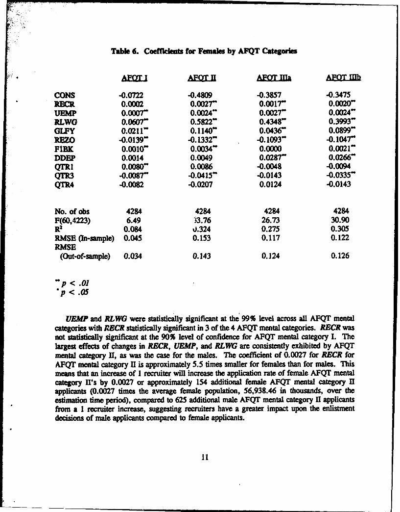
Table 6. Coeff ntetas for Females by AFQT Caterles

A= IE AEQLUH AEQIJr MMQL lb

SCONS -0.0722 -0.4809 -0.3W7 -0.3475RECR 0.0002 0.002r 0.0017" 0.0020"UEMP 0.OOO7" 0.0024" 0.0027r 0.O24"RLWG 0.060r 0.5822" 0.4348" 0.3993"nOLFY 0.0211" 0.1140" 0.0436" 0.0899"REZO -0.0139" -0.1332" -0.1093" -0. l04wFIBK 0.0010" 0.0034" 0.0000 0.0021"DDEP 0.0014 0.0049 0.028r 0.0266Cqrll 0.00oo"o 0.0086 -0.0048 -0.0094QTR3 -0.0087" -0.0415" -0.0143 -0.0335"QTR4 -0.0082 -0.0207 0.0124 -0.0143

No. of obs 4284 4284 4284 4284F(60,4223) 6.49 33.76 26.73 30.90R2 0.084 J324 0.275 0.305RMSE (In-sample) 0.045 0.153 0.117 0.122RMSE

(Out-of-sample) 0.034 0.143 0.124 0.126

"p < .01

"p < .05

UFMP and RLWG were statistically significant at the 99% level across all AFQT mentalcategories with RBCR statistically significant in 3 of the 4 AFQT mental categories. RECR wasnot statistically significant at the 90% level of confidence for AFQT mental category I. Thelargest effects of changes in RECR, UEMP, and RLWG are consistently exhibited by AFQTmental category U, as was the case for the males. The coefficient of 0.0027 for RECR forAFQT mental category 11 is approximately 5.5 times smaller for females than for males. Thismeans that an increase of 1 recruiter will increase the application rate of female AFQT mentalcategory I's by 0.0027 or approximately 154 additional female AFQT mental category I1applicants (0.0027 times the average female population, 56,938.46 in thousands, over theestimation time period), compared to 625 additional male AFQT mental category II applicantsfrom a 1 recruiter increase, suggesting recruiters have a greater impact upon the enlistmentdecisions of male applicants compared to female applicants.

11i

The coefficient for UEMP for AFQT mental category Mila, 0.0027, implies that ifunemployment declines by 0.5 percentage points, then the application rate for AFQT mentalcatWory [Ia's will decline by 0.001 or approximately 77 fewer female AFQT mental category[la's will apply to the Air Force. AFQT mental categories II and MIb had the same value for

the UEilP coefficient, 0.0024, which is not statistically different from the UEMPcoefficient forAFQT mental category Ula.

The coefficient for RLWG for AFQT mental category I, 0.5822, implies that if the relativemilitary to civilian wage declines by 0.05 points, then the application rate for female AFQTmental category IU's will decline by 0.0029 (0.5822 times 0.05) or approximately 166 fewerfemale AFQT mental category U's will apply to the Air Force. The relative wage elasticity forAFQT mental category U1 females of 1.984, is approximately 1.87 times as large as the relativewage elasticity for male AFQT mental category II's. The wage elasticities for female AFQTmental categories I's, la's, and tub's are 2.012, 2.131, and 1.783, respectively. Theseelasticities are generally higher than the elasticities presented for males. This implies that forany AFQT category, females tend to be more responsive to changes in relative military to civilianwages than males, possibly owing to the fewer realized employment opportunities of femaleyouths compared to male youths.

Caucasians

Table 7 presents the OLS estimates for Caucasian MEPS applicants. The coefficients varyacross AFQT categories with AFQT mental category I, once again, having consistently smallercoefficient values. UEMP and RECR were statistically significant at the 99 % level across AFQTmental categories, RLWG was statistically significant in all of the AFQT mental categories. Thelargest effects of changes in RECR, UEMP, and RLWG were consistently for AFQT mentalcategory II, as was the case for the males and females.

The coefficient of 0.0080 for RECR for AFQT mental category II means that an increase of1 recruiter will increase the applia'ion rate of Caucasian AFQT mental category U's by 0.0080or approximately 668 additional Cja-asian AFQT mental category U1 applicants (0.0080 timesthe average Caucasian population, 83,560.18 in thousands, over the estimation time period). Thecoefficient for UEMP for AFQT mental cate'ory II, 0.0131, implies that if unemploymentdeclines by 0.5 percentage points, then the application rate for AFQT mental category U's willdecline by 0.0065 or approximately 547 fewer Caucasian AFQT mental category U's will applyto the Air Force.

The coefficient for RLWG for AFQT mental category II of 0.6607, implies that if the relativemilitary to civilian wage were to decline by 0.05 points, then the applicaion rate for CaucasianAFQT mental category II's would decline by 0.0330 (0.6607 ti.es 0.05) or approximately 2,760fewer Caucasian AFQT mental category IT' -ill appty to the Air Force. The relative wageelasticity for AFQT mental category 11 Caucasians was calculated to be 0.926. The wageelasticities for Caucasian AFQT mental categories I's, HIa's, and tub's were 0.882, 1.338, and0.717, respectively.

12

Table 7. Coefficients for Caucasian by AFQT Categories

AFOT I EAFQ I AFOT AaFOT I

CONS -0.0618 -0.3938 -0.3644 -0.1263RECR 0.0012" 0.0080" 0.0039" 0.0045"UEMP 0.0013" 0.0131" 0.0060" 0.0055"RLWG 0.0784" 0.6607" 0.5316" 0.2827"GLFY 0.0426" 0. 1987" 0.0581" 0.0883"REZO -0.0468" -0.3395" -0.2288" -0.2332"FIBK 0.0018" 0.0046" -0.0002 0.0019DDEP 0.0028 -0.0177" 0.0245" 0.0242"QTR1 0.0048 -0.0283 -0.0058 -0.0034QTR3 -0.0271" -0. 1437" -0.0529" -0.0719"QTR4 -0.0241" -0.0457 0.0183 -0.0098

No. of obs 4284 4284 4284 4284F(60,4223) 14.24 58.92 56.57 64.79R 0.168 0.456 0.446 0.479RMSE (In-sample) 0.061 0.241 0.152 0.159RMSE

(Out-of-sample) 0.059 0.263 0.162 0.190

"p < .01"p < .0 5

Blacks

Table 8 presents the OLS estimates of Black MEPS applicants for the Air Force. Thecoefficients vary across AFQT mental categories with AFQT mental category I, once again,having consistently smaller coefficient values. RECR is statistically significant at the 99% levelof confidence for AFQT mental categories 1I, Mlia, and rob, while AFQT mental category Iexhibits statistical significance at the 92 % level of confidence. UEMP is statistically significantat the 99% level of confidence for only one AFQT mental category, Mlb, while AFQT mentalcategory MIa exhibits statistical significance at the 92% level of confidence. AFQT mentalcategories I and II had statistically insignificant coefficients for UEMP. RLWG is statisticallysignificant at the 99% level of confidence for AFQT mental categories II and Mia, while slightlyless than a 90% level of confidence for AFQT mental categories I and IITb.

13

• •, • • • i I ! I I I 'WJ

Table S. Coefficients for Blacks by AFQT Categories

MAEQIJF ELUl

CONS -0.0546 -0.8966 -0.7264 -0.5376RECR 0.0003 0.0055- 0.0062" 0.0124-UEM -0.0001 0.0001 0.0013 0.0031"RLWG 0.0493 1.0488" 0.8445" 0.5756GLFY 0.0021 0.0719 0. 1727" 0.4255"REZO -0.0148" -0.2184" -0.2756" -0.4608"FlBK 0.0004 0.0015 0.0061" 0.0125"DDEP 0.0032 -0.0224" 0.0314" 0.0127QTRI 0.0047 -0.0069 -0.0105 -0.0216QTR3 -0.0032 -0.0246 -0.0697" -0. 1353"QTR4 -0.0061 0.0291 -0.0497 -0.0732

No. of obs 2100 2100 2100 2100F(34,2065) 1.19 16.10 17.30 24.71R2 0.019 0.210 0.222 0.289RMSE (In-sample) 0.037 0.213 0.261 0.409RMSE

(Out-of-sample) 0.042 0.223 0.231 0.435

"p < .01"p < .05

The largest coefficient for RECR occurs for AFQT mental category 11b, 0.0124, whichimplies that an increase of 1 recruiter will increase the application rate of Black AFQT mentalcategory 1Db by 0.0124, or approximately 335 additional Black AFQT mental category TUbapplicants (0.0124 times the average Black population, 27,046.98 in thousands, over theestimation time period). The largest coefficient for UEMP is for AFQT mental category Ilb,0.0031, which implies that if unemployment declines by 0.5 percentage points, then theapplication rate for AFQT mental category mb will decline by 0.0016, or approximately 42fewer Black AFQT mental category ED will apply to the Air Force.

The largest coefficient for RLWG is for AFQT mental category 1, 1.0488. This coefficientimplies that if the relative military to civilian wage declines by 0.05 points, then the applicationrate for Black AFQT mental category U's will decline by 0.0524 (1.0488 times 0.05), orapproximately 1,418 fewer Black AFQT mental category II's will apply to the Air Force. Thecoefficient for RLWG and the sample means for RLWG and the dependent variable (application

14

rate for Black AFQT mental category I's) results in a relative wage elasticity of 2.589. Thewage elasticities for Black AFQT mental categories I's, MIa's, and IIb's are 3.397, 1.604, and0643, respectively.

Others

Table 9 presents the OLS estimates of Other (non-Caucasian, non-Black) MEPS applicantsfor the Air Force. The coefficients vary across AFQT mental categories with AFQT mentalcategory I, once again, having consistently smaller coefficient values. RLWG is statisticallysignificant at the 99% level of confidence for AFQT mental category HIlb and at the 90% levelof confidence for AFQT mental category lIa.

Table 9. Coefficients for Others by AFQT Categories

AFQI AFQrII AFOT HIa AFOTIJI k

CONS 0.3015 -0.8353 -2.3262 -3.8543RECR -0.0016 -0.0073 0.0003 -0.0020UEMP -0.0013 -0.0009 0.0056 -0.0033RLWG -0.1935 1.1677 2.4128 3.9613"GLFY 0.0339 0.5299 -0.2218 0.4051REZO 0.0741 -0.5143 -0.7450 -0.9327"FIBK 0.0043 0.0280 0.0086 -0.0190DDEP 0.0854" 0.9235"* 0.9220" 1.1559"QTR1 -0.0037 -0.2024 -0.3467 -0.2353QTR3 -0.0127 -0.3655 -0.2834 0.0834QTR4 -0.1136 -0.4211 -0.4275 0.58990

No. of obs 672 672 672 672F(17,654) 2.95 16.10 19.26 31.35R2 0.071 0.295 0.334 0.449RMSE (In-sample) 0.334 1.377 1.424 1.562RMSE

(Out-of-sample) 0.517 1.887 1.803 1.956

"p < .01"p < .05

15

The largest coefficient for RLWG is for AFQT mental category r1b, 3.9613. This coefficientimplies that if the relative military to civilian wage declines by 0.05 points, then the applicationrate for other AFQT mental cateiory Ihlb's will decline by 0.1981 (3.961295 times 0.05), orapproimately 878 fewer other AFQT mental category MIb's will apply to the Air Force(3.961295 times 0.05 times the average other population, 4433.02 in thousands, over theestimation time period).

AU

Table 10 presents the OLS estimates of all (includes all gender and race groups) MEPSapplicants. The coefficients vary across AFQT mental categories with AFQT mental categoryI, once again, displaying consistently smaller coefficient values. The magnitude of the effectsof economic and recruiting factors on the decision of AFQT mental category I to join the AirForce relative to the other AFQT mental categories is not unexpected. AFQT mental categoryI would be expected to have the highest opportunity cost of the AFQT mental categories,especially with respect to attending college.

Table 10. Coefficients for All by AFQT Categories

AFOT AIQ II AFOTIia AFQT IID

CONS -0.0700 -0.6460 -0.5962 -0.5632RECR 0.0010" 0.0075" 0.0043" 0.0057"UEMP 0.0012"* 0.013r" 0.0083" 0.0085"RLWG 0.0803" 0.8320" 0.6665" 0.5724"GLFY 0.0430" 0.2407" 0. 1136" 0. 1843"REZO -0.0395" -0.3035" -0.2343" -0.2541"F1BK 0.0020" 0.0072*0 0.0022" 0.0063"DDEP 0.0057" 0.0008 0.0406" 0.0368"QTR1 0.0049 -0.0126 0.0067 0.0168QTR3 -0.0250"" -0.1406" -0.0569" -0.0834"QTR4 -0.0250" -0.0604" 0.0040 -0.0390

No. of obs 4284 4284 4284 4284F(60,4223) 18.80 61.43 57.61 69.57R2 0.211 0.466 0.450 0.497RMSE (In-sample) 0.055 0.226 0.152 0.173RMSE

(Out-of-sample) 0.054 0.242 0.167 0.211

"p < .01"p < .05

16

URW , RLWG, and RECR were statistically significant at the 99% level across all AFQTmental categories. The largest effects of changes in RECR, URMP, and RLWG are consistentlyexhibited by AFQT mental category IU, as was the case for the males and females. Thecoefficit for RECR of 0.0075 means that an increase of I recruiter will increase the applicationrate of all AFQT mental category U by 0.0075 or approximately 743 additional AFQT mentalcategory II applicants (0.0075 times the average youth population, 99,186.77 in thousands, overthe estimation time period).

The coefficient for UEMP for AFQT mental category U, 0.0137, implies that ifunemployment declines by 0.5 percentage points, then the application rate for AFQT mentalcategory II will decline by 0.007 or approximately 694 fewer AFQT mental category u's willapply to the Air Force. The coefficient for RLWG for AFQT mental category II, 0.8320,implies that if the relative military to civilian wage declines by 0.05 points, then the applicationrate for all AFQT mental category U's will decline by 0.0416 (0.8320 times 0.05) orapproximately 4,126 fewer AFQT mental category U's will apply to the Air Force.

Elasticities

The elasticities with respect to recruiters (RECR), unemployment (UEMP), and relativemilitary to civilian wages (RLWG) vary significantly between demographic groups and aptitudegroups within demographic groups. Tables 11, 12, and 13 present the elasticities for RLWG,UEMP, and RECR, respectively. The elasticities are calculated using Equation 4.

Relative Military to Civilian Wage Elasticity. The relative wage elasticities (RLWG)presented in Table 11, reveal that Blacks tend to show the highest relative wage elasticity. Thesehigher wage elasticities suggest that Black youths have fewer realized employment opportunities,and are therefore more sensitive to changes in military compensation relative to civiliancompensation compared to Caucasian youths. Females had higher wage relative wage elasticitieswhen compared to males. This also suggests that female youths have fewer realized employmen,opportunities when compared to male youths, thus making them more sensitive to changes inrelative military to civilian compensation.

AFQT mental category UIb's tend to have lower relative wage elasticities across alldemographic groups. The low relative wage elasticities for AFQT mental category HUb's couldbe the result of recruiters discouraging potential low aptitude applicants from advancing to theMEPS stage of the application process. This implies that the recruiter is able to assess aptitudeon the basis of other information besides actual AFQT scores.

Unemployment Elasticity. The unemployment elasticities displayed a similar range ofvariation across demographic and aptitude groups as did the relative military to civilian wageelasticities (Table 12). The unemployment elasticities for Caucasian youths and male youthssuggest that on average Caucasians and male youths are more responsive to changes in theunemployment rate. Males have historically shown a higher propensity to apply for militaryservice than females, and thus when the unemployment rate increases, males tend to have a

17

larger increase in their application rates for military service compared to females. The relativelyfewer job opportunities for females in the military also causes the female application rate to beless responsive to changes in the unemployment rate compared to males.

Table 11. Relative Wage Elasticities for Demographicand Aptitude Groups

Demographic AFQT AFQT AFQT AFQT

Group Cat I Cat IH Cat Mla Cat I1lb

Males 0.792 1.062 1.504 1.146

Females 2.012 1.984 2.131 1.783

Caucasians 0.882 0.926 1.338 0.717

Blacks 3.397 2.588 • 1.604 0.643

Others -1.646 0.769W 1.653 2.009

All 0.999 1.210 1.559 1.205

Note: Values annotated by I are statistically insignificant (below the 90% level of confidence)

Table 12. Unemployment Elasticities for Demographicand Aptitude Groups

Demographic AFQT AFQT AFQT AFQT

Group Cat I Cat 11 Cat Ilia Cat IIlb

Males 0.116 0.152 0.137 0.126

Females 0.250 0.087 0.140 0.113

Caucasians 0.146 0.183 0.151 0.138

Blacks -0.166" 0.0060 0.060 0.085

Others -0.2288 -0.012" 0.0788 -0.0344

All 0.175 0.234 0.227 0.210

Note: Values annotated by 8 are statistically insignificant (below the 90% level of confidence)

18

Recruiter Elastkcty. The recruiter elasticities presented in Table 13 also vary acrossde .ograIc and aptitude groups but not with the level of variation displayed by the relativemilitary to civilian elasticities and the unemployment elasticities. With the exception of females,the recruiter elasticities across all demographic groups tend to suggest that the impact of arecruiter is the largest for higher aptitude (AFQT mental category I) compared to lower aptitude(AFQT mental categories II and Ella) youths.

Table 13. Recruiter Elasticities for Demographicand Aptitude Groups

Demographic AFQT AFQT AFQT AFQT

Group Cat I Cat 1H Cat ma Cat IIlb

Males 0.781 0.665 0.618 0.748

Females 0.375& 0.507 0.453 0.489Caucsin 0.737 0.614 0.540 0.619

Blacks 1.745 1.153 1.000 1.176

Others -0.950. -0.333a 0.014A -0.070r

All 0.705 0.596 0.544 0.653

Note: Values annotated by are statistically insignificant (below the 90% level of confidence)

Explanatory Credibility of Equations

The R2s were strong for males and Caucasians in AFQT mental categories H, EIla, and m1Tb,as shown in Table 14. All equations were statistically significant (F-value) with the exceptionof Black/AFQT mental category I. AFQT mental category I consistently had the lowest R2sacross demographic groups. AFQT mental category I also had the smallest number of applicants.For example, the mean number of applicants across states presented in Table 15 for males,AFQT mental category I was 5.9, while the means for males, AFQT mental categories II, lila,and MIb were 49.1, 29.3, and 33.2, respectively. Similar patterns were exhibited by females(1.5 for AFQT Category I), Caucasians (7.0 for AFQT mental category I), and Blacks (0.4 forAFQT mental category I). Blacks equations, in general, had low Rs (Table 14), but they alsohad low application rates, as well as having sufficient data for analysis of only 25 states.

An out-of-sample projection was made for the calendar year 1990 and compared with actualapplication rates. The root-mean-square errors (RMSE) are presented for both in-sample andout-of-sample projections in Table 16. The out-of-sample RMSEs are only slightly larger than

19

their in-sample counterparts. The RMSE's for the AFQT mental category I's tend to be largerthan the sample means of the dependent variables (Stone et al., 1991).

Table 14. R's for Equations

Aptitude/ AFQT AFQT AFQT AFQTDemographic Category Category Category Category

Group I n MIa IIlb

Males 0.174 0.409 0.383 0.451

Females 0.084 0.324 0.275 0.265

Caucasians 0.168 0.456 0.446 0.479

Blacks 0.0199 0.210 0.222 0.289

Others 0.071 0.295 0.334 0.449

All 0.211 0.466 0.450 0.497

Note: Value annotated by a is statistically insignificant (below the 90% level of confidence)

Table 15. Sample Means for Application Numbers

Aptitude/ AFQT AFQT AFQT AFQTDemographic Category Category Category Category

Group I II EIa 1b

Males 5.9 49.1 29.3 33.2

Females 1.5 15.2 10.9 12.3

Caucasians 7.0 56.8 31.2 30.9

Blacks 0.4 11.1 14.2 24.3

Others 0.6 7.3 6.5 8.7

All 7.4 64.3 40.1 45.6

20

Table 16. In-Sample and Out-of-Sample RMSEs

Aptitude/ AFQT AFQT AFQT AFQT

Demographic Category Category Category CategoryI.Group 1 11 MRl MJb

Males - In 0.108 0.429 0.290 0.339

Males - Out 0.118 0.444 0.296 0.383

Mean" 0.152 1.251 0.750 0.838

Females-In 0.045 0.153 0.117 0.122

Females - Out 0.034 0.143 0.124 0.126

Mean 0.030 0.301 0.210 0.230

Caucasians - In 0.061 0.241 0.152 0.159

Caucasians - Out 0.059 0.263 0.162 0.190

Mean 0.091 0.733 0.408 0.405

Blacks - In 0.037 0.213 0.261 0.409

Blacks - Out 0.042 0.223 0.231 0.435

Mean 0,015 0.416 0.541 0.920

Others - In 0.334 1.377 1.424 1.562

Others - Out 0.517 1.887 1.803 1.956

Mean 0.119 1.540 1.481 2.000

All - In 0.055 0.226 0.152 0.173

All - Out 0.054 0.242 0.167 0.211

Mean 0.083 0.706 0.439 0.488

"Sample mean of the dependent variable.

Summary of Estimation Results

The coefficients for number of recruiters (RECR), unemployment (UEMP), and relativemilitary to civilian wage (RLWG) were statistically significant at the 99% level of confidence for

21

males (relative military to civilian wage, AFQT mental category I - 98%), females (number ofrecruiters, AFQT mental category I - insignificant), and Caucasians. The coefficients for Blackswere insignificant for recruiters for AFQT mental category I, for unemployment AFQTcategories I, II, and MIIa, and for relative military to civilian wage in the case of AFQT mentalcategories I and Ulb.

The R2s were strong for males and Caucasians, AFQT mental category U's Ulia's, and lllb's,Table 14. All equations were statistically significant (F-value) with the exception of black/AFQTmental category I's. AFQT mental category I's consistently had the lowest R2s acrossdemographic groups. The out-of-sample RMSEs, for most demographic groups, are only slightlylarger than their in-sample counterparts. The RMSE's for the AFQT mental category I's tendto be larger than the sample means of the dependent variables.

The relative military to civilian pay elasticities were similar in range to other studies, butdiffered significantly across demographic and aptitude groups. On average, a 1% increase in therelative military to civilian wage will increase the rate of application by approximately 1.00%for AFQT mental category I's, 1.21% for AFQT mental category I's, 1.56% for AFQT mentalcategory MIa's, 1.21 % for AFQT mental category Itub's.

The unemployment elasticities also varied significantly across demographic and aptitudegroups. On average, a 1 % increase in the unemployment rate will increase the rate ofapplication by approximately 0.18 % for AFQT mental category I's, 0.239% for AFQT mentalcategory U's, 0.23 % for AFQT mental category ha's, 0.21 % for AFQT mental category THb's.

The recruiter elasticities differed across demographic and aptitude groups but not with thelevel of variation displayed by the relative military to civilian elasticities and the unemploymentelasticities. On average, a 1% increase in the number of recruiters will increase the rate ofapplication by approximately 0.71% for AFQT mental category I's, 0.60% for AFQT mentalcategory U's, 0.54 % for AFQT mental category lIla's, 0.65 % for AFQT mental category UIb's.

IMPLEMENTATION OF THE DEMOGRAMIC MODELS INTO AAPS

The Am, zan Applicant Prediction System (AAPS) is a user friendly, menu-driven softwarepackage which provides the user with the ability to analyze the rate of flow of variousdemographic groups into the MEPS for Air Force entry (Fast, Stone, Turner, Looper, andEngquist, 1991). The applicant equations developed in this study were implemented into AAPSto improve the predictability of AAPS and extend the level of analysis in AAPS from aggregateto the state/region level. AAPS begins with a user specified available (A) youth population(e.g., 17 to 21 year old male Caucasians) and proceeds to determine the numbers of the youthpopulation that are military available (MA), interested military available (IMA), interestedqualified military available (IQMA), and MAGE stratification of the IQMA population.

22

SMilitary Available

In AAPS, the population data for each state is maintained as a proportion of the totalpopulation across states in order to minimize internal memory requirements. Thus, AAPS beginsby determining the proportion of the total population for theJth state, Pj, and the total populationN. Of course, there will be a population N for each projection year, 1995 to 2010. Thefollowing discussion is for a single projection year but is extendable for multiple projection years.Population projections were obtained from the Bureau of the Census for 16 to 26 year olds byrace and gender for the time period 1988 to 2010.

The analysis begins with the user selected available population as defined by gender, race,and age which is equal to the summation of the state level available population to produce N.The next step in the analysis is the estimation of the portion of the available population whichis institutionalized. The proportion of any selected population which is institutionalized isassumed to be equal to a constant. The level of the institutionalized population can be modifiedby the user. The proportion of the available population which is institutionalized in each state,PI times Pj times N, redefines N to be

N x (0-Pi) = N (6)

whereN* - number of the non-institutionalized population andP- - proportion of the available population which is institutionalized (Spencer,

1989).

The next step in the analysis is to define the number of high school diploma graduates in thepopulation. This is defined as the proportion of non-institutionalized population in each state,J, expected to receive degrees times the non-institutionalized population, N*. To determine thenumber of high school graduates for each state, HSDGj, then:

HjxPjxN* = HSDGj (7)

whereHj - proportion of high school degrees conferred for statej andPj - proportion for statej of the total available population.

Proportions of each states population with high school degrees were obtained from the U.S.Department of Education, National Center for Education Statistics (based on Fall 1986enrollments). Thus, the state proportions which must be carried forward to the next step in theanalysis of the population are

23

HSD

E HSDGj()

where the denominator of Equation 8 is the number of high school graduates.

The number of the selected non-institutionalized population who are already in the service iscalculated next. The number of armed service members is equal to the proportion of the non-

stitutonalzed population of each state in-service times the proportion of population in eachstate, J, times the non-institutionalized population, Nf. This can be expressed as

4jX Pj XN = SVCJ (9)

where/j - proportion of in-service members in the non-institutionalized population by

statej andSVCj - number of armed service members for each state.

Proportions of the non-institutionalized population in-service by state were obtained from Bureauof the Census projections of resident Armed Forces populations for 1988 to 2010. Thus, thestate proportions which must be carried forward to the next step in the analysis are

svc.PJsv (10)

J-1

where the denominator of Equation 10 is the number of people already members of the ArmedForces.

The number of the non-institutionalized population who have prior military service is the nextcalculation. The number of prior service members in the non-institutionalized population is equalto the proportion of prior service in the population times the proportion of the non-institutionalized population of each state times the non-institutionalized population. Theproportion of prior service in the population is assumed to be constant across states, thus, varyingby a constant proportion of the state population. This can be expressed as

PS xP xN = PRSJ (11)

24

PS - proportion of pror service members in the non-institutioaid PoPulation,r, and

PRSj - number of prior service members for each state.

The proportions for the prior service population were based on a study by Verdugo and Berliant(1968). The state proportions which must be carried forward in the analysis become

PJPRS (12)

Ji-

where the denominator in Equation 12 is the number of prior service members for the selectedpopulation.

The number of college students in the population is calculated next. The number of collegestudents in the non-institutionalized population is equal to the proportion of college students inthe population of statej times the proportion of the non-institutionalized population of each statetimes the non-institutionalized population which can be expressed as

CXPj xN* = COLJ (13)

whereC - proportion of college students in the non-institutionalized population (Verdugo

and Berliant, 1988), N, andCOLj - number of college students for each state.

The state proportions which must be carried forward in the analysis are

e•,•OL = jo. (14)E COLJJI

where the denominator of Equation 14 is the number of college students in the selected non-institutionalized population.

The calculation of the MA population must exclude the institutionalized population, non-highschool graduates, number of active armed service members in the population, number of priorservice members in the population, and number of college students in the population. Excludingthe number of non-high school graduates from the population is particularly relevant for the Air

25

¾I

Force, though other branches of the Department of Defense (DoD) may consider accessing non-high school graduates. The exclusion of non-high school graduates is also relevant for thepresent recruiting environment in which the demand for accessions has declined significantly dueto force•downsizing. Thus, the MA for statej is equal to

MAj = (pj.=WxN*)-(Pjs3 cxN*)- (P p, ~x N ) - (j,r..oL x N)(I

+ (Pi, RS X Pj, COL X NI

To continue the analysis of the selected population, the state proportions which must be carriedforward to the next step in the analysis are

PJMA - (16)

IJMJ-1

where the denominator of Equation 16 is the number for military available and Pjm, is theproportion which will be used continue to the analysis of IMA. The original Pj will no longerbe used beyond this point of the population analysis.

Interested Military Available

The calculation of the Interested Military Available (IMA) uses the MA population todetermine the number of interested AFQT mental category I's, IH's, 1Ila's, and Mub's in the MApopulation. The empirical results from the Estimation of Demographic Models section are usedto estimate the number interested in each of the AFQT mental categories. For example, thenumber of interested military available AFQT mental category I's in the MA population is equalto the proportion of AFQT mental category I's in state j of the population (estimated from theempirical results of the previous section) times the proportion of the MA population in state jtimes the MA population. The proportion of AFQT mental category k applicants in statej, P,can be expressed as

Pj,k = aOJ,k + lJ,ktRECR + cL2 J, UEMP + (17)

a 3 jkRLWG + a 4,iSTj7k

26

wherle

4W - intercept term for theJth state and the kth AFqr mental category from

the empirical results of the estimations presented in the previous section(Equation 3). The coefficients for the variables GLFY, REZO, FIBK,DDEP, QTRM, QMR3, and QTR4, have been included in the interceptterm,

Go0.* - the cth coefficient for the jth state and the kth AFQT mental category

from the empirical results of the estimations presented in the previoussection,

STjA - binary variable for thejth state and the kth AFQT mental category, and

values for RECR, UEMP, and RLWG may be specified by the user. The number of interestedmilitary available (IMA) in the kth AFQT mental category for each state, IMACATjA, can thenbe calculated and expressed as

IMACAT., = eJk XPJJ( xMA (18)

wherePA& - proportion of the kth AFQT category in state j of the population,PNA - proportion of military available (MA) in state j of the MA population, andMA is the military available population from the original selected population.

The state proportions which have been maintained to this point of the analysis are no longerrequired for the rentining population analysis. The number of IMACATjA collapses across statesfor each Ath category and will be maintained for the next steps of the analysis. IMACAT, canbe expressed as

J

The calculation for AFQT mental category I's, I's, .ila's, and llIb's follows the same methodas the calculation for AFQT mental category k. The only factor which changes is the proportionof specific AFQT mental category in statej of the population which is derived from the empiricalresults of the previous section.

The calculation of the total IMA population is equal to the sum of the calculations forAFQT mental category I's, I's, lia's, and MIb's. This can be expressed as

IMA = IMA CA T, + IMA CA T,7 + IAL,4 CA T17 + IMA CA T= (20)

27

or

JAM = IMACAT, (21)k=!

Interested Qualified Military Available

The Interested Qualified Military Available (IQMA) requires the exclusion of three groupsfrom the population: those who do not meet the AFQT mental category requirements, those whoare not medically and/or morally qualified, and those who do not meet the minimum enlistmentstandards for the Air Force based on the general (G) composite score and the sum of the fourcomposite scores: general, mechanical (K), administrative (A), and electronic (E). Forexample, the Air Force presently requires that an applicant possess a G score of 60 or better anda summed composite score of 180 or better to qualify for the Air Force. This represented theminimum enlistment standards for the Air Force at the time of this study.

To determine the number of AFQT qualified in the selected population, the numbers fromeach AFQT mental category designated as qualified are summed together. For example, ifAFQT mental category I and AFQT mental category II have been designated as qualified, thenAFQT Qualified will equal the sum of the numbers for AFQT mental category I and AFQTmental category II from the IMA population.

The number medically and morally qualified from the IMA population is equal to theproportion of medically and morally qualified applied to each AFQT mental category selectedas qualified. Thus, MMQ,, the number of medically and morally qualified, can be determinedfor each qualified AFQT mental category k by

X

MMQ = E (MMxIMACATk) (22)k-I

whereMM - proportion of medically, morally qualified (AF/MPZ Special Study Team,

1985),IMACATk - number of IMA population that is AFQT mental category k, andMMQ - medically and morally qualified population of the IMA population.

Thus, MMQ is the number of medically and morally qualified population.

The enlistment standards qualified (ESQ population which meets the minimum G score andsummed Composite is equal to the proportion applied to each AFQT mental category selected

28

as qualified. Thus, ESQt, the enlistment standards qualified for AFQT mental category k canbe expresed as

ESQ (ESQk xIMACATk) (23)k-I

whereESQ - proportion of the AFQT mental category k which meets the enlistment

standards of G score and Composite,IMACAT, - number of interested military available AFQT mental category k from

the IMA population, andESQ - population of AFQT mental category qualified which meets the enlistment

standards of G score and summed Composite.ESQ. was based on matrices in which each cell of the matrix represents the proportion

of the MEPS population for FY90 MEPS data which possessed those M, A, G, and E scores.For example, one of the matrix cells could represent all applicants who had an M score of 50,an A score of 80, a G score of 70, and an E score of 40. There was a matrix for each AFQTmental category (I through MIb) and each cell of the matrix represented a decile combination ofscores. In order to calculate the proportion of ESQ for the kth AFQT Category, the ratioequaled the number of applicants in the relevant cells (cells identified as qualified, meeting boththe G score minimum and the summed Composite minimum) divided by total number ofapplicants in the kth matrix. For example, if the user selected AFQT mental categories I andII, the matrices for k= 1 and k=2 are used to calculate the proportion of each matrix which isESQ, ESQ1 and ESQ3 .

Thus, the calculation of IQMA from the population of IMA can be expressed as

IQMA = E [(MM xESQk)xIMACATk] (24)k-I

whereMM - proportion of medically, morally qualified (AF/MPZ Special Study Team,

1985),ESQk - proportion of the AFQT Category k which meets the enlistment standards

of G score and summed Composite,IMACAT& - number of interested military available AFQT mental category k from

the IMA population, andIQMA - population of interested military available population which is qualified

from the IMA population.

29

'Tus, IQMA is the number interested qualified military available from the selected population.In addition, the number of interested military available population which is qualified from theIMACATk population, IQMtA, must be maintained for the next stage of the analysis. lQXAkis equil to

IQMAt = (MMxESQt)xIMACATk (25)

The MAGE Distribution of the IQMA Population

MAGE Distribution of IQMA uses the same MAGE matrices applied in the calculation ofIQMA. However, n will be calculated using the sum of the restricted cells of the matrices(restricted by the enlistment standards and by the AFQT mental categories selected)

IQMAMAGE - (sQRkxIMACATk) (26)k-i

whereESQ&R is the proportion of the AFQT mental category k which meets the

designated MAGE standards,10MAt is the number of interested military available population which is qualified

from the IMACATk population, andIQAAMAGE is the population of interested qualified military available population

which meets the designated MAGE standards.

AIRMAN APPLICANT PREDICTION SYSTEM SOFTWARE

The preceding section discussed the components of the Airman Applicant Prediction System(AAPS). In this section, the mechanics of using and operating the software for AAPS will bediscussed. AAPS allows a user to predict the number of qualified applicants for Air Forceservice from a given demographic population. The user may specify census, economic, andavailability constraints within AAPS. AAPS begins with a user specified demographicpopulation, and then determines the available (A), military available (MA), interested militaryavailable (IMA), and interested qualified military available (IQMA) population for thespecified demographic group(s). The IQMA population may then be queried to determine thenumber of applicants that meet minimum ASVAB composite score requirements.

Census Constraints

AAPS first allows a user to specify the population from which a projection will be made. Byspecifying census constraints the user may specify a national prediction (all states), a regionalprediction (all states within the specified regions), or a state prediction (any combination of

30

states). The user may also specify the racial and gender groups to be included in the prediction.The user may choose from Caucasians, Blacks, or others (or any combination of the three) andfrom males or females (or both). Population data are available for 17 to 26 year olds in each

- demographic group. The user may also specify the age groups to be included in the prediction.Cmsus coestraints also allow the user to specify the time period for the prediction, with the years1995 to 2010 available. After selecting a population for the prediction, the user is ready to eitherchange the economic or availability constraints, or to use the Forecast option to obtain thepedictions.

Economic Constraints

Economic constraints allow the user to specify changes in the unemployment rate, the ratioof military to civilian wages, or the recruiting resources. Unemployment rates may be changedby state or across states, as well as by demographic groups or across demographic groups. Theratio of military to civilian wages may be changed by state or across states. Recruiting resources(number of recruiters) may also be changed by or across states. After changing the economicconstraints, the user is ready to either change the availability constraints or to use the Forecastoption to obtain the predictions.

Availability Constraints

Availability constraints allow the user to specify military availability constraints and qualifyingavailability constraints. Military availability constraints determine the proportion of thepopulation that will be excluded from the MA population because they are institutionalized, in-service, have prior service, or are in college. The user may change the proportion of thepopulation that are in any of these categories. The user may also specify the proportion of theIMA population that will medically and morally qualified for military service.

Qualifying availability constraints allow the user to specify enlistment qualifications. The usermay determine if a high school diploma is required for applicants to be considered qualified, andmay also specify the proportion of the population in each state which will have a high schooldiploma. The AFQT mental categories which will be considered as qualified for enlistment mayalso be specified (categories I, 11, MIa or 1ib). The user may also specify the minimumenlistment standards, minimum General and Composite scores, for all apphicants to be consideredqualified. After specifying the availability constraints, the user may then use the Forecast optionto obtain the predictions.

Forecasting Predictions

The Forecast option allows the user to obtain the predictions of the A, MA, IMA, and IQMApopulation for the chosen demographic groups. The A population is the predicted number ofyouths for the chosen demographic and age groups for all specified states by year. The MApopulation predictions are obtained by removing the institutionalized, non-high school degree (ifspecified), in-service, prior service and college populations from the A population. The

31

empirical results of the estimations of this study are then used to predict the numbers ofapplicants (IMA) by AFQT mental category from the MA population. AFQT mental category,medical and moral, and enlistment standard qualifications are then applied to the IMA populationin order to obtain the IQMA population. The user may then specify minimum ASVABcomposite scores, mechanical (M), administrative (A), general (G), and electronic (E), requiredfor applicants. AAPS will then predict the number of applicants meeting this minimum scorerequirements from the IQMA population.

The user has the option of printing any of the prediction tables or viewing graphs of thetables. The user may also save the tables created from the predictions. At this time the usermay return to the census constraints and create new predictions or exit the package.

CONCLUSIONS

The Estimation of the Demographic Models section presented the results of the estimation ofthe state level demographic models using pooled time series, cross-sectional data. Three of thedemographic groups provided models which exhibited strong statistical results considering resultsgenerally obtained from pooled time series, cross-sectional analyses and compared to previousstudies by Cotterman (1986) and Goldberg and Goldberg (1988). Coefficients and theirelasticities presented in Section IV are comparable to Cotterman (1986) and Goldberg andGoldberg (1988) results, though only the Goldbergs performed analysis for the Air Force.

Several key features differentiate the study presented in Section IV from previous studies.Cotterman (1986) and Goldberg and Goldberg (1988), as well as other analysts use contracts, notapplicants, in the numerator of the dependent variable to represent the rate of accession. Thenumber of contracts in a given month for the Air Force are driven primarily by recruiting goalswhich have been met on a monthly basis for the past several years (at least since 1983). Thus,using contracts to represent the actual flow of people seeking employment in the Air Force ismodeling a constrained and predictable flow. Air Force Recruiting Service can predict withnearly 100% accuracy the number of accessions in each month of fiscal year 1992. Applicantsare a much better representation of a market driven supply, affected by the normally acceptedmarket factors of military to civilian wages, recruiters, and employment.

In addition, this study not only analyzes the flow of male high school graduates, but includesfemales, Caucasians, Blacks, and others. In addition, the analysis further categorizes thesedemographic groups by AFQT categories I, II, lIra, and rob.

The specification of the equations included variables to account for recruiting effort beyondthe number of production recruiters. GLFY represents how well the Air Force was performingrelative to the fiscal year NPS accession goal. For each monthly time period, t, it representedhow well the Air Force had attained its fiscal year enlistment goal through time period 9-1.REZO was a binary variable for the three month time period during November 1989 to January1990 (REZO - 1) when recruiters were not allowed to issue contracts to recruits due to the large

32

fonce drawdowns required to meet end-of-fiscal-year force level requirements. FIBK is avariable which represents the number of recruits in the DEP for the "next" fiscal year.

Even with the specification of these other recruiting factors in the equation, the variable forthe number of production recruiters was still statistically significant in 18 of the 24 equations.In addition, due to this level of detail in the equation specification, the coefficients for recruiterhad a much better chance of representing the actual effect of recruiters on the application flow.

The estimation results presented in this study can be summarized with several key points. Therelative military to civilian pay elasticities were similar in range to other studies, but differedsignificantly across demographic and aptitude groups. The unemployment elasticities also variedsignificantly across demographic and aptitude groups. The recruiter elasticities differed acrossdemographic and aptitude groups but not with the level of variation displayed by the relativemilitary to civilian elasticities and the unemployment elasticities.

Coefficients for number of recruiters (RECR), unemployment (UEMP), and relative militaryto civilian wage (RLWG) were statistically significant at the 99% level of confidence for males(relative military to civilian wage, AFQT mental category I - 98 %), females (number ofrecruiters, AFQT mental category I - insignificant), and Caucasians. Blacks exhibitedinsignificance for recruiters for AFQT mental category I, for unemployment for AFQT mentalcategories I, II, and lia, and for relative military to civilian wage in the case of AFQT mentalcategories I and Rib.

The R2s for the equations were strong for males, Caucasians and all, AFQT mental categoryU's Ila's, and Rib's. All equations were statistically significant (F-value) with the exception ofBlack/AFQT mental category I's. AFQT mental category I's consistently exhibited the lowestR2s across demographic groups. The out-of-sample RMSEs are only slightly larger than theirin-sample counterparts. The RMSE's for the AFQT mental category I's are consistently largerthan the sample means of the dependent variables. This implies that the equations did as wellpredicting in-sample as they did out-of-sample.

The results of the estimation of this study were implemented in the Airman ApplicantPrediction System (AAPS) software. AAPS is user-friendly, menu-driven, PC compatiblesoftware package which may be used to predict the applicant flow of selected demographicgroups at the national, regional, or state level. The estimated coefficients of the equations areused to predict the number of a military available (MA) population that would be interested inapplying for Air Force service by AFQT mental category.

33

REFERENCES

AF/MPZ Special Study Team (1985). The Prospects for Military Enlistment. An Assessment.In coordination with Syllogistics Inc. and Unicon Research Corporation,Washington, DC.

Becker, G.S. (1971). Economic Theory. New York: Alfred A. Knopf.

Cotterman, R.F. (1986). Forecasting Enlistment Supply: A lime Series of ross SectionsModel (R-3252-FMP). Santa Monica, CA: The RAND Corporation.

Curtis, E.W., Borack, J.I., & Wax, S.R. (1987). Estimating the Youth PopulationQuali(tedfor Military Service (NPRDC TR-87-32). San Diego, CA: Navy PersonnelResearch and Development Center.

Dale, D., & Gilroy, C. (1984). Determinants of Enlistments: A Macroeconomic Time-seriesView. Armed Forces & Society, 10(2), 192-210.

Daula, T.V., Fagan, T.W., & Smith, D.A. (1982). A Microdata Model of Enlistmentin the Armed Forces. Paper presented at the summer meeting of the EconometricSociety, Ithaca, NY.

DeVany, A.S., & Saving, T.R. (1982). Life-cycle Job Choice and the Demand and Supplyof Entry Level Jobs: Some Evidence from the Air Force. Review of Economics andStatistics, 64(3), 457-465.

Fast, J.C., Stone, B.M., Turner, K.L., Looper, L.T., & Engquist, S.K. (1991). CvilianAvailability Model (AL-TP-1991-0028). Brooks AFB, TX: Manpower and PersonnelResearch Division, Human Resources Directorate.

Goldberg, L., & Goldberg, B.S. (1988). Analysis of Military Enlistments in the 1980s (MDA903-87-C-0790). Washington, DC: Office of the Assistant Secretary of Defense,(FM&P/MM&PP) Accession Policy, Pentagon.

Hosek, J.R., & Peterson C.E. (1985). Enlistment Decisions of Young Men (R-3238-MIL).Santa Monica, CA: The RAND Corporation.

House, D.R., Saving, T.R., & Stone, B.M. (1985a). Employment of Recent Dental Graduates:Phase 11. Paper prepared for Department of Health and Human Services, by RRC, Inc.,Bryan, TX.

House, D.R., Saving, T.R., & Stone, B.M. (1985b). Impact of Dental Prepayment on theDemand for Dental Care. Paper prepared for Research Triangle Institute for theDepartment of Health and Human Services, by RRC, Inc., Bryan, TX.

34

Orvis, B.R., & Gahart, M.T. (1985). Relationslup of Enlistment Interti on and Market Surveyljbnnlon to Enlistment in Active Duty Mili:ary (N-2292-MIL). Santa Monica, CA:Te RAND Corporation.

Orvis, B.R., & Gahart, M.T. (1989). Quality-ased Analysis Capability for National YouthSwurves: Development, Application, and Implications for Policy (R-3675-FMP).Santa Monica, CA: The RAND Corporation.

Orvis, B.R., Gahart M.T., & Hosek, J.R. (1989). Predicting Enlistmentfor Recruiting MarketSegments (N-2852-FMP). Santa Monica, CA: The RAND Corporation.

Saving, T.R., Battalio, R.C., DeVany, A.S., Dwyer, G.P., & Kagel, J.K. (1980, June). AirForce Enlisted Personnel Retention-Accession Model (AFHRL-TR-80-12). Brooks AFB,"TX: Manpower and Personnel Division, Air Force Human Resources Laboratory.

Saving, T.R., & Stone, B.M. (1983, September). Air Force Prior Service Market Analysis.Washington, DC: AFMPXOA, Pentagon.

Spencer, G. (1989). Projections of the Population of the United States, by Age, Sex, and Race:1988 to 2080. Current Population Reports, Population Estimates and Projections. SeriesP-25, No. 1018. Washington, DC: U.S. Department of Commerce, Bureau of theCensus.

Stone, B.M., Saving, T.R., Turner, K.L., Looper, L.T., & Engquist, S.K. (1991). ASimultaneous Estimation Model ofAir Force Accession and Retention. Brooks AFB, TX:Manpower and Personnel Division, Air Force Human Resources Laboratory.

U.S. Department of Education (1986). High School Graduation Rates. Washington, DC:National Center for Education Statistics.

Verdugo, N., & Berliant, K.R. (1988). Estimating the Army's Prime Recruiting Market (TR-832). Alexandria, VA: U.S. Army Research Institute for the Behavioral and SocialSciences.

35

APPENDIX

The state level population projections within the Airman Applicant Prediction System (AAPS)must be periodically updated. AAPS currently contains population projections for the year 1988through 2010. These population projections were obtained from the United States Departmentof Commerce, Bureau of the Census, and are consistent with those published in *Projections ofthe Population of States by Age, Sex, and Race: 1989 to 2010", Current Population Rqeorts,Series P-25, No. 1053.

Updated population projections should also be obtained from the Bureau of Census.Projections of state populations by single years of age, sex and race which are consistent withthose published in the Current Pulation R=r=, Series P-25, No. 1053 should be requestedfrom:

Mr. Larry SinkStatistical Information StaffPopulation DivisionBureau of the CensusWashington, D.C. 20233(301) 763-1902

These data are available on diskette for purchase.

AAPS contains population projections from projection series C for the ages 16 to 26 yearsof age. To update the population file for AAPS, a file must be created which contains theconcatenated state population files for all 51 states obtained from the Bureau of the Census. Thisfile should be in the following format:

Vab I= gth Values

State char 2 state postal codesYear num 4 19xx - 20xxRace num 1 1 = caucasians

2 = blacks3 = other

Sex num I I = males2 = females

Popl6 num 6 population age 16Popl7 num 6 population age 17

Pop26 num 6 population age 26

36

This file should be named STATEDAT and should be used to replace the current STATE.DATfile presently used by AAPS. The starting and ending years of the population projections mustalso then be changed within AAPS, The years must be changed within the BROBJ.PAS file.The variable MiNYEAR must be set equal to the year of the first population projection withinthe STATEDAT file. The variable MAXYEAR must be set equal to the year of the lastpopulation projection within the STATE.DAT file. AAPS will now predict using the newpopulation projections.

37