A SURROGATE APPROACH TO THE EXPERIMENTAL OPTIMIZATION

OF MULTIELEMENT AIRFOILS

John C. Otto�

Multidisciplinary Optimization BranchNASA Langley Research Center

Hampton, VirginiaDepartment of Aeronautics and Astronautics, M.I.T.

Drew Landmany

Department of Engineering TechnologyOld Dominion University

Norfolk, Virginia

Anthony T. Pateraz

Department of Mechanical EngineeringMassachusetts Institute of Technology

Cambridge, Massachusetts

AIAA Paper 96{4138{CP

American Institute of Aeronautics and Astronautics

Abstract

The incorporation of experimental test data into theoptimization process is accomplished through theuse of Bayesian-validated surrogates. In the surro-gate approach, a surrogate for the experiment (e.g.,a response surface) serves in the optimization pro-cess. The validation step of the framework providesa qualitative assessment of the surrogate quality, andbounds the surrogate-for-experiment error on designs\near" surrogate-predicted optimal designs. The util-ity of the framework is demonstrated through its ap-plication to the experimental selection of the trailingedge ap position to achieve a design lift coe�cientfor a three-element airfoil.

Introduction

To address the inherent di�culties in examiningmany design points experimentally, a three-elementairfoil model with internally embedded actuators hasbeen developed.1 The model (Fig. 1) has a nestedchord of c = 18 in., a span of b = 36 in., and was de-signed for low-speed testing in several local tunnels,

�Research Scientist, Member AIAAyAssociate Professor, Member AIAAzProfessor

Copyright c by the American Institute of Aeronautics and As-

tronautics, Inc. No copyright is asserted in the United States

under Title 17, U.S. Code. The U.S. Government has a royalty-

free license to exercise all rights under the copyright claimed

herein for Governmental Purposes. All other rights are re-

served by the copyright owner.

Main ElementFlap

Slat

Actuator Flap Bracket

y

x

Figure 1: Three-element model with internal ap actuators.

including the NASA Langley Research Center 2- by4-foot and the Old Dominion University (ODU) 3- by4-foot low-speed facilities. The main element chordis cmain = 14:95 in., and the ap and slat chords(expressed as a percentage of the nested chord) are30 and 14.5 percent, respectively. The ap and slatare both de ected to 30� for all tests. Although thisparticular model is suitable only for low Reynoldsnumber testing, the techniques developed should beapplicable to higher Reynolds number testing as well.

The ap actuators are computer controlled and po-sition the ap horizontally and vertically (x and y,respectively). The model has been used in the ODUtunnel to compile baseline values for lift coe�cientCl versus ap gap and overhang at �xed angles ofattack and slat riggings. A �rst-order optimizer thatuses a variant of the method of steepest ascent2;3 hasbeen demonstrated in real time.4 The capability ofthe computer controller to automatically take data

1

https://ntrs.nasa.gov/search.jsp?R=20040110894 2018-05-14T09:23:33+00:00Z

at a prescribed set of (x; y) coordinates makes thissetup ideal for the surrogate methods described next.

The Bayesian-validated surrogate framework ap-plied in this paper provides a practical means to in-corporate experimental data directly into the designoptimization process. In the surrogate approach tooptimization, a surrogate (i.e., a simpli�ed model,for example a response surface) for the experiment isconstructed from o�-line appeals to the experiment.The surrogate is then used in subsequent optimiza-tion studies. This approach to optimization can becontrasted with on-line (direct insertion) strategies,in which appeals to the experiment are embedded di-rectly into the optimization process.

The o�-line surrogate approach5�8 to optimizationo�ers several advantages to on-line approaches. First,by construction, surrogates are computationally in-expensive and are thus easily incorporated into op-timization procedures. Additionally, the low com-putational requirements create a highly interactiveand exible design environment, which allows the de-signer to easily pursue and examine multiple designpoints. Second, the number of appeals to the experi-ment or simulation is known a priori, which ensuresthat the design can be accomplished without exhaust-ing available resources. Third the surrogate approacho�ers a natural means to incorporate data from pre-vious runs and/or other sources.

As regards disadvantages, the primary drawback isthat in high dimensional design spaces, surrogate con-struction is di�cult and design localization is poor. Asecond limiting factor in the application of the surro-gate approach to experimental tests is the need tovalidate the surrogate at input points chosen ran-domly in the design space. This capability, present inthe experiment central to this work, is not typical ofmost experimental tests. Finally, surrogate-based op-timization introduces a new source of error. The sur-rogate validation strategy and error norms discussedin this paper seek to quantify the discrepancy be-tween the surrogate and the experiment by providingestimates to the system predictability and optimality.

In this paper, we �rst describe the experimentalmodel and the testing methods used. Second, wepresent the optimization problem that is central tothe work. Third, we brie y describe the three stepsof the baseline surrogate framework (i.e., construc-tion/validation, surrogate-based optimization, and a

posteriori error analysis), summarize the inputs tothe framework, and then present an overview of themore sophisticated surrogate algorithms. Finally, wepresent sample results obtained from the surrogateframework for output maximization and multiple-target designs, and compare the surrogate approach

+

Gap

Overhang

Flap

Main Element

Figure 2: De�nition of gap and overhang.

with the direct insertion results reported previously.4

Experimental Testing Methods

An important practical problem encountered in wind-tunnel testing of multielement airfoils is the need totest a range of con�gurations to ensure that the op-timum is selected. Unfortunately, this testing canbe prohibitively time consuming if one considers allpossible variables, such as ap position and de ec-tion, slat position and de ection, overall angle of at-tack, and Reynolds number. For example, a range of ap locations and orientations relative to the mainelement is typically tested. In a cryogenic or pres-surized facility, model geometry changes necessitatelarge delays in testing. These delays often result ininvestigators choosing a sparse test matrix and an op-timum that is based on only a few points. The abilityto move the ap under computer control provides aunique opportunity to explore the entire range of use-ful gap and overhang values (Fig. 2).

In this experiment, the ap actuators, tunnel owsetting, and data acquisition were controlled by a per-sonal computer running Lab View9 software. A pro-gram was written to allow any number of ap posi-tions (in x and y) to be sampled in any order. Windtunnel power was controlled such that at the begin-ning of each test the tunnel was restarted to avoidhysteresis e�ects.4 The experimental setup allowedthe user to start the program, which at each loca-tion in turn automatically measured the free-streamproperties, sampled and recorded pressures aroundthe centerline of the model, and then calculated liftcoe�cients for the three-element airfoil. This processrequired approximately 2 min. for each data point.

Two typical pressure distributions are shown inFigure 3, where the ordinate is the pressure coe�-cient Cp and the abscissa is distance from the leadingedge expressed as a percent of the nested chord. Thedata for Figure 3(a) represents a point near the peakCl for this con�guration, and the plot in Figure 3(b)

2American Institute of Aeronautics and Astronautics

4 12 20 28 36 44 52 60 68 76 84 92

x/c %

0 8 16

-6

-5

-4

-3

-2

-1

0

1

2

Cp

68 76 84 92 100

gaps = 2.17

o.h.s = -1.46

x=14.75 y=.25

α = 8°Cl = 2.04

Re = 1x106

Slat Main Element Flap

0 8 16

-6

-5

-4

-3

-2

-1

0

1

2

Cp

68 76 84 92 100

Slat Main Element Flap

α = 8°Cl = 2.72

Re = 1x106

gaps = 2.17

o.h.s = -1.46

x=14.55 y=.45

4 12 20 28 36 44 52 60 68 76 84 92

x/c %

(a) Fully attached ow over all elements.

(b) Detached ow over the ap.

Figure 3: Experimental pressure data.

indicates full separation over the ap.

Test matrices were developed to survey ap po-sitions, which ranged from approximately 0:8 { 3:5percent (gap) and �0:4 { 3:4 percent (overhang) rel-ative to the nested chord c. Two angles of attackand two slat geometries were selected. An angle ofattack � of 8� was chosen as representative of an ap-proach value. An � of 14� represented the limit ofgood-quality two-dimensional ow for the ODU tun-nel installation without tunnel wall boundary-layercontrol. Two slat settings were chosen: a slat gap of3:03 percent with an overhang of 2:46 percent and,for a smaller gap setting, a slat gap of 2:17 percentwith a slat overhang of �1:46 percent

Positional accuracy was enhanced by requiring thatthe ap move to a reference point above and be-hind the desired evaluation points (xref > xeval,yref > yeval ) and then back to the evaluation point.This eliminated any e�ect of backlash in the mechan-ical drive-train. Two simple tests provided an indi-cation of the inherent collective error due to instru-mentation and positioning. The �rst test involvedtwo separate evaluation points; the �rst point was

in a region in which the ow was known to be fullyattached to all elements, and the second point waschosen in a region in which ow over the ap wasfully separated. The positioning program was usedto move the ap between a reference point and oneof the evaluation points. The tunnel was restartedbefore every evaluation, and the test was repeated 30times in each case. The standard deviation of Cl wasfound to be 0:004 for the separated case (0.16 per-cent) and 0.0118 for the attached case (.36 percent).For the second test, the program automatically sam-pled 29 points over the entire test region for two dif-ferent trials. The error in Cl between the two runsaveraged 0.71 percent with a standard deviation of0.75 percent. Although these tests are not exhaus-tive, they do provide a benchmark for the Cl error.The turbulence intensity in the ODU tunnel was

measured at less than 0.2 percent. Flow quality overthe model was monitored through 12 spanwise taps: 6on the ap, and 6 on the main element. The ow wasconsidered to be two-dimensional if the magnitude ofthe spanwise nonuniformity was less than 5 percentof the total Cp variation over the entire model.

10 Thedata presented are uncorrected for boundary e�ectswere taken at a Reynolds Re number of 1�106 basedon the nested chord.

Optimization Problem

We begin by introducing a vector p of M designinputs that lie in the input (or \design") domain � IRM , an input-output function S(p) : ! IR,and an objective function (S(p);p; �) that charac-terizes our design goals, where � is a vector (or possi-bly scalar) design parameter. For the work presentedhere, we set p = (x; y) (the x- and y-positions of the ap) as the M = 2 inputs and restrict ourselves toan input domain of reasonable ap positions (de-scribed in more detail in the results section). The out-put of interest is the lift coe�cient, S(p) = Cl(x; y).The objective function is (S(p);p; �) = jS(p) � �jwhich has been referred to as the \discrimination"problem.11

With the above terms de�ned, the minimizer p� =(x�; y�) to the exact optimization problem is given by

p� = argminp2

jS(p) � �j : (1)

In this formulation, the goal is to �nd that (or \an")input vector p� = (x�; y�) that achieves as closely aspossible the target lift coe�cient value �. If the tar-get lift coe�cient � is set su�ciently small (large), theformulation describes the output minimization (max-imization) problem, assuming that S(p) is boundedfrom below (above).

3American Institute of Aeronautics and Astronautics

In the on-line approach, the experiment is invokedat every optimization step needed to solve Equation(1). In the o�-line approach, a surrogate, eS(p) �S(p), for the experiment is inserted into the opti-mization problem. The minimizer, ep� = (ex�; ey�), forthe resulting, surrogate-based, discrimination prob-lem is then given byep� = argmin

p2j eS(p)� �j : (2)

Here, the optimization proceeds exactly as it wouldfor the on-line approach, but the lift coe�cient surro-gate eS(p) is invoked instead of the experiment. Thesurrogate problem that corresponds to Equation (1),but with a general objective function (S(p);p; �),has been reported by Ye�silyurt12 and Ye�silyurt andPatera.8

Surrogate Framework

The advantages to pursuing a surrogate-based ap-proach to optimization have already been described.However, to use a surrogate-based approach with con-�dence in a design setting, the issues of predictabil-ity and optimality must be addressed.13 For pre-dictability, the concern is with how the actual ex-periment performs in the vicinity of the surrogate-predicted minimizer ep�. If the surrogate-predictedminimizer is to be of value, we must be able to boundjS(p0) � S(ep�)j for p0 \near" ep�, and this boundmust be acceptably small. In the case of optimality,the designer requires con�dence that the surrogate-predicted optimizer ep� is near the \exact" optimizer,that is, ep� � p�. Optimality requires stronger as-sumptions in regard to the form of the objectivefunction (e.g., quasi-convexity) and is, therefore, dif-�cult to determine in real applications. Optimal-ity is, however, an important consideration and, al-though not addressed further here, has been exam-ined elsewhere.8;12

The distinguishing attribute of the Bayesian-validated surrogate methodology is that a com-plete and rigorous validation step is fully inte-grated into the a posteriori error analysis of thesurrogate-predicted design(s). The approach de-scribed here is related to probably-approximately-correct approaches14;15 and information-based com-plexity theory.16 The surrogate approach di�ers,however, from the former in that it is truly non-parametric (no assumption is made in regard to thedistribution of ep�) and from the latter in that it re-quires no regularity estimates for the input-outputfunction.The surrogate approach is broken into three steps.

In the �rst stage, surrogate construction/validation,

experimental results and/or prior information are

used to construct the approximation, eS(p) � S(p);additional queries to the experiment are used to val-idate the approximation. In the second step of theprocess, surrogate-based optimization, solutions tosurrogate optimization problem of Equation (2) areobtained. In the third and �nal step, a posteri-

ori error analysis, the results of the validation areused to analyze the consequences of the surrogate-for-simulation substitution. In the following subsections,we describe the three steps of the baseline surrogateframework, summarize the inputs to the framework,and review the more sophisticated surrogate algo-rithms.

Construction/Validation

We construct the lift coe�cient surrogate eS(p) =A(X co) � S(p) using an approximation scheme,A : (IRM ; IR)N

co

! L1() and a construction sam-ple set of input-output pairs

X co = f(pi; Rpi); i = 1; : : : ; N cog ; (3)

where Rpi = Cl(xi; yi) is a realization of the experi-mentally measured lift coe�cient for the input apposition pi = (xi; yi), and N co is the number ofinput-output pairs in the construction sample. Al-though the general surrogate framework can handlenoisy outputs,17 the noise contribution is neglected inthe work presented in this paper. Information fromprior studies, outside sources, or asymptotic behav-ior can also be incorporated into the approximationprocess. It is important to note that the surrogateframework makes no assumptions in regard to theapproximation technique and will accept, and assess,any approximation A(X co). Also, no restriction isplaced on either N co or the distribution of the con-struction sample.To proceed with the description of the surrogate

validation, we �rst introduce the importance function�(p). The importance function serves as a probabilitydensity function for the selection of the validationpoints: Z

�(p)dp = 1: (4)

The importance function also leads to the notion of a�{measure associated with �(p): for any subdomainD � ,

��(D) =

ZD

�(p)dp < 1: (5)

The �{measure of D is simply the weighted relativeM -volume of D.

4American Institute of Aeronautics and Astronautics

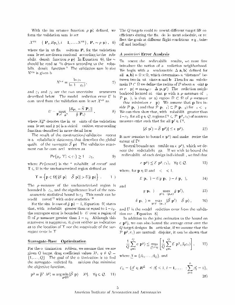
With the importance function �(p) de�ned, weform the validation sample set

X va = f(Pi; RPi); i = 1; : : : ; Nvag ; Pi � �(p) ; (6)

where the input ap positions Pi for the validationsample set are drawn randomly according to the prob-ability density function �(p). In Equation (6), the �should be read as \is drawn according to the proba-bility density function." The validation sample sizeNva is given by

Nva =ln "2

ln(1� "1); (7)

and "1 and "2 are the two uncertainty parametersdescribed below. The model prediction error U iscomputed from the validation sample set X va as

U = maxPi2X

vaP

jRPi� eS(Pi)j

g(Pi); (8)

where X vaP denotes the input points of the validation

sample set and g(p) is a strictly positive, error-scalingfunction described in more detail later.The result of the construction/validation process

is a probabilistic statement that describes the globalquality of the surrogate eS(p). The validation state-ment can be compactly written as

Prf��(�) < "1g � 1� "2; (9)

where Prfeventg is the \probability of event" and� � is the uncharacterized region de�ned as

� =np 2 j jS(p)� eS(p)j > Ug(p)

o: (10)

The �{measure of the uncharacterized region isbounded by "1, and the signi�cance level of the non-parametric statistical bound is "2. This result can bereadily proved12 with order statistics.18

For the simple case of g(p) = 1, Equation (9) statesthat, with probability greater than or equal to 1�"2,the surrogate error is bounded by U over a region of of �{measure greater than 1 � "1. Although thisstatement is suggestive, it gives neither an indicationas to the location of � nor the magnitude of the sur-rogate error in �.

Surrogate-Based Optimization

For the optimization problem, we assume that we aregiven Q target drag coe�cient values �q ; q 2 Q =f1; : : : ; Qg. The goal of the optimization is to �ndthe surrogate-predicted ap positions that minimizethe objective function,

pq = ep�(�q) = argminp2

j eS(p)� �q j; 8q 2 Q: (11)

The Q targets could represent di�erent target lift co-e�cients during the ap deployment schedule, or re- ect the goals at di�erent ight conditions (e.g., take-o� and landing).

A posteriori Error Analysis

To present the predictability results, we must �rstintroduce the notion of a prediction neighborhood.We begin with a pseudometric �(a;b) de�ned forall (a;b) 2 �, which determines a \distance" be-tween two input points a and b. Then for any subdo-mainD � we de�ne the radius of D about a point pas rD(p) = maxp02D�(p;p0). The prediction neigh-borhood located at point p with a �{measure of z,P(p; z), is that (or a) region D � of �{measurez that minimizes rD(p). We assume that p lies in-side P(p; z) and that P(p; z1) � P(p; z2) for z1 < z2.We can then show that, with probability greater than1�"2, for all q 2 Q, regions �

q � P(pq; "1) of nonzeromeasure exist such that for all p0 2 �q,

jS(p0)� eS(pq)j � e(pq): (12)

It now remains to bound e(pq) and make precise theextent of �q.Several bounds are possible on e(pq), which we de-

note the predictability gap. If we wish to bound thepredictability of each design individually, we �nd that

e(pq) � E(pq ; "1); 8q 2 Q; (13)

where, for p 2 and 0 < z < 1,

E(p; z) = Ug(p; z) + �(p; z); (14)

andg(p; z) = max

p02P(p;z)g(p0); (15)

�(p; z) = maxp02P(p;z)

j eS(p0)� eS(p)j; (16)

and U is the model prediction error from the valida-tion step, Equation (8).In addition to the joint estimates to the bound on

e(pq), we can also bound the average error over theQ target designs. In particular, if we assume that theP(pq; "1) are mutually disjoint, it can be shown that

1

Q

QXq=1

e(pq) � max�2CQ

"1

Q

QXq=1

E(pq ; �q"1)

#; (17)

where � = f�1; : : : ; �Qg, and

CL = f�0 2 IRLj0 � �0l � 1; l = 1; : : : ; L;

LXl=1

�0l = 1g;

(18)

5American Institute of Aeronautics and Astronautics

is the set of convex L{tuples. The \nonparametricaverage" is relevant to multiple-target designs andrepresents the average, as opposed to the worst-case,estimate of the predictability. Also, it is importantto note that this predictability bound is calculatedentirely in terms of the inexpensive surrogate, eS(p).Finally, for a successful validation (i.e., ��(�) <

"1), we can bound the expectation of the size of �q

with respect to the validation sample joint probabilitydensity. The resulting bound is, 8q 2 Q,

E

���(�

q)

"1j ��(�) < "1

�� 1 +

1

ln "2+

"2

(1� "2):

(19)The expression in Equation (19) bounds the average�{measure of the region �q, with respect to "1, formany validations.

Several advantages to bounding the errors only towithin a �nite uncertainty exist.19 First, we achieve asense of stability in that the estimates apply not onlyto a single point, but to regions �q of nonzero mea-sure, assuring that many input points pq exist thatsatisfy the error estimates. Second, for the multiple-target case the estimates become sharper becausethere is only a single uncharacterized volume of mea-sure "1. Equation (17) is the upper bound for thedistribution of the single "1-sized uncharacterized re-gion among the Q designs. This analysis results ina bound on the average error which is less than theaverage of the individual predictability gap boundsE(pq ; "1). Finally, because our predictability analy-sis is not premised on any particular set of points,the designer has exibility in the choice of the metric�(a;b) (discussed further in the next section).

As mentioned in the introduction, the primarydrawback to the surrogate approach is the di�cultconstruction and validation of the surrogate in highdimensional input spaces. We can easily illustratethis point if we consider the uniform importance func-tion �(p) and a neighborhood of �{measure "1 in theinput domain = [0; 1]M . The neighborhood will

span at least "1=M1 in one of the input directions which

rapidly approaches one asM !1. The loss of local-ization as M ! 1 produces a corresponding loss inpredictability through �(p; "1) in Equation (14). Incertain instances, the surrogate approach can be ef-fectively applied to problems with high dimensionalinput spaces. This includes cases in which the in-puts are highly correlated (e.g., for shape optimiza-tion where highly oscillatory geometries are not likelyoptimizers20) or specialized formulations apply (e.g.,Pareto formulations21). In general however, the sur-rogate approach is restricted to a moderate numberof design variables.

Summary of Surrogate Inputs

To summarize the surrogate framework description,and to highlight the exibility of the environment, wenote that four inputs to the process are determinedby the user. These are listed below:

i. An importance function �(p) : ! IR+.

ii. An error-scaling function g(p) : ! IR+.

iii. Two uncertainty parameters, "1 and "2, that sat-isfy 0 < "1; "2 < 1.

iv. A pseudometric �(a;b).

Each input provides the designer with exibility, andallows the designer's experience to impact and im-prove the �nal surrogate-predicted designs. Althoughpoor choices for the inputs do not in uence the valid-ity of the surrogate results, they greatly reduce thesharpness of the results. A short description and ex-planation of each input follows.The importance function �(p) re ects the designers

prejudices in regard to the regions of that are morelikely to contain optimizers. In this context, �(p)is essentially a \prior" on ep�. To serve this purpose,�(p) is used as the probability density function in therandom selection of validation points in Equation (6).A judicious choice of �(p) (one that is large in the re-gions of the �nal designs and small elsewhere) cansigni�cantly increase the sharpness of the a posteri-

ori error bounds. The increased sharpness is a conse-quence of much better physical localization (in termsof input variable extent) of the prediction neighbor-hood P(ep�; "1), which in turn reduces the surrogatesensitivity contribution �(ep�; "1) to the error boundin Equation (14).The error-scaling function g(p) can be used by the

designer to reduce the impact of localized surrogateerrors on the error bounds of the �nal design. Be-cause the model prediction error U in Equation (8) isglobal, a large value of g(p) in regions for which theapproximation is poor will result in a reduced valueof the �rst term on the right-hand side of Equation(14), provided that the �nal design does not lie in aregion where g(p) is large.The uncertainty parameters "1 and "2 are related

to the number of validation points through Equation(7). This formula allows the precise budgeting of re-sources and ensures that useful solutions can be ob-tained. In e�ect, Equations (7){(10) describe what isknown in a continuous sense about a function basedon discrete sampling. Analysis of Equation (7) showsthat, asymptotically for small "1 and "2, Nva in-creases linearly as "1 decreases and only logarithmi-cally as "2 decreases. This relationship suggests that

6American Institute of Aeronautics and Astronautics

although we can easily (in terms of validation samplesize) increase our con�dence in the results (smaller"2), re�ning the localization of our results (throughsmaller "1) is much more di�cult. The localizationhas a direct impact on the �nal error analysis through�(p; "1) in Equation (14). The relative di�culty infurther re�ning the localization illustrates the needto intelligently select �(p) and where appropriate,�(a;b), both of which can have similar e�ects onthe localization error.The �nal input to the surrogate approach is the

pseudometric �(a;b). Because �(a;b) can be chosenpost-validation, various metrics can be examined, andthe most appropriate selected. One possible trade-o� is between design localization (in terms of inputvariable extent) and predictability in terms of �(p; "1)in Equation (14). An example of the extreme of thistrade-o� is the sensitivity minimizing metric

�(a;b) = j eS(a)� eS(b)j (20)

used for the single-point design study of the resultssection. This metric gives the lowest possible �(p; "1).

Improved Algorithms

Several, more sophisticated surrogate algorithmshave been developed8;12;17;19�23 but are not de-scribed here. First, a surrogate formulation for noisyoutputs has been developed.17 This formulation isclearly appropriate in an experimental setting butis not addressed here. Second, the multiple outputcase can be e�ciently handled, and the formulationcan be applied to model selection. Third, elemen-tal decompositions of are possible that yield lo-cal errors and allow for rigorous construction/cross-validation schemes.24 Fourth, sequential and adap-tive techniques have been developed that allow theincremental deployment of resources to achieve tar-get surrogate accuracies and that more tightly couplethe construction and validation phases of the baselinealgorithm. Finally, nested validation, in which a hi-erarchy of models exists (e.g., an extremely expensive\truth" model! a high-�delity model! low-�delitymodel), has been addressed as well.

Results

To demonstrate the surrogate framework, we haveapplied it to the experimental design of multielementairfoils; speci�cally, we are interested in determin-ing the optimal location for the trailing edge ap,based on the lift coe�cient Cl in low-speed, high-lift ight regimes. The M = 2 design inputs to the prob-lem p = (x; y) are the x and y positions of the ap,

measured from the leading edge of the main airfoilelement and normalized by the main element chordcmain = 14:95 in. The output of interest is Cl. In ad-dition, several other con�guration and ow conditionparameters are �xed for the study. These parametersare listed in Table 1 and are the Reynolds number Re,the airfoil angle of attack �, the ap and slat de ec-tion angles �flap and �slat, respectively, and the gapand overhang of the slat (expressed as a percentageof the nested chord c = 18:0 in.).In this section, we �rst describe the method used

for the surrogate construction and report the vali-dation results. Second, we consider the single-pointdesign problem of output maximization. Third, wepursue a multiple-target design study which demon-strates the increased sharpness of the nonparametricaverage error results. Finally, we report the resultsof on-line optimization studies and compare these re-sults with the o�-line, surrogate results.

Surrogate Construction/Validation

The construction sample set X co consists of 119input-output pairs that are uniformly spaced on a17 � 7 grid. The (x; y) ap positions for the con-struction sample are plotted as circles in Figure 4.The input domain is divided into three subdomains, = 1 [ 2 [ 3, based on the ow conditions overthe ap. In the �rst subdomain 1, the ow overthe ap is attached, with the exception of the ex-treme aft positions in which some trailing-edge sepa-ration may be present (and desirable). In this region,a radial basis function25 serves as the approximationmethod, which yields the surrogate eS1(p). In 3, the ow over the ap is fully separated, and a second ra-dial basis function �t serves as the surrogate eS3(p).In 2, the resolution of the construction points isnot su�cient to determine the precise location of theseparation line. In this region, a simple linear tri-angulation between eS1(p) and eS3(p) is used as the

surrogate, eS2(p). The error function, g(p), is set tounity in 1 and 3, and g(p) = 50 in 2, re ect-ing our uncertainty in regard to the location of the

Re 1; 000; 000� 14�

�flap 30�

�slat �30�

gapslat 2:17%overhangslat �1:46%

Table 1: Fixed design study parameters.

7American Institute of Aeronautics and Astronautics

0.96 0.97 0.98 0.99 1.00 1.01

.02

.03

.04

y

x

Construction points

1

2

3

= 1 [ 2 [ 3

Figure 4: Surrogate construction points andthe input (\design") domain.

separation line and, hence, our lack of con�dence inthe quality of the surrogate in this region of the in-put space. A three-dimensional surface plot of thesurrogate is shown in Figure 5.

To validate the lift coe�cient surrogate, we mustselect a set of random input points in and run theexperiment at each of these points to form the valida-tion sample set X va. The input points are con�nedto the design space described in the previous para-graph and shown in Figure 4. Because the construc-tion data were obtained simultaneously with the vali-dation data, we had no expectation in regard to thoseregions of the input space that would be of most inter-est; thus, we used a uniform probability density func-tion �(p) for the selection of the validation points.We budgeted Nva = 45 points for validation and, us-ing the relationship in Equation (7), set "1 = 0:03and "2 = 0:25. If we had known the form of the sur-rogate prior to taking the validation data, we couldhave restricted the design space to a more feasible re-gion and perhaps chosen an importance function �(p)that would have concentrated validation points closeto potential designs. The scaled model prediction er-ror computed according to Equation (8) is U = :0482.Note that the maximum un-scaled error does in factoccur in 2 as we presupposed and has a value of0:4824. If we had chosen g(p) = 1 everywhere (in-stead of as described above), our model prediction er-ror would have been approximately one order of mag-nitude larger, and would surely have overwhelmed theresults.

The surrogate just described and the related vali-dation results serve for all of the designs discussed inthe remainder of this paper. One primary advantageto using the surrogate approach is the fact that noadditional experimental data are required to boundthe errors of future designs that are pursued withthe surrogate. This characteristic, combined with

the negligible computational time required for eachsurrogate evaluation, yields a highly exible designenvironment that does not sacri�ce predictability.

Single-Point Design, Surrogate Maximization

For the �rst study, we pursue a single-point designthat maximizes the surrogate output. We set � su�-ciently large in Equation (2) and minimize the result-ing function. To accomplish the optimization, we usethe unconstrained quasi-Newton optimizer that is in-cluded in the optimization toolbox of Matlab26. Theresulting surrogate-based optimizer is located at ep� =(x�; y�) = (:997; :036), and the surrogate-predicted

lift coe�cient value at this point is eS(ep�) = 3:388.The optimizer was started with an initial guess atp0 = (:987; :033) and required 44 surrogate evalua-tions to arrive at ep�. Because the surrogate is inex-pensive to evaluate (and because we are working withonly two inputs and can visualize the results graphi-cally), we can verify that we do achieve a surrogate-predicted global maximum. This veri�cation wouldbe more di�cult in a purely on-line optimization set-ting if we did no begin the optimizer at multiple start-ing points p0 until we had su�cient con�dence thata global maximum had been obtained.Finally, we choose the sensitivity minimizing met-

ric �(a;b) � j eS(a) � eS(b)j in Equation (20) andperform the a posteriori error analysis for a single-point design. We construct the prediction neighbor-hood P(ep�; "1) around ep� and �nd the surrogate sen-sitivity parameter � = :0328. The optimal point ep�and the associated prediction neighborhood P(ep�; "1)are plotted in Figure 6. The resulting predictabil-ity statement reads as follows: with con�dence levelgreater than :75, a region � � P(ep�; "1) of nonzeromeasure exists such that for all p0 2 �

jS(p0)� eS(ep�)j � e(ep�) ; (21)

where

e(ep�) � Ug(ep�; "1) + � = :0810 : (22)

We see that the predictability is relatively good withrespect to the surrogate-predicted maximum lift co-e�cient, but quite poor with respect to the range oflift coe�cients of interest (i.e., corresponding to appositions in 1).

Multiple-Target Designs

For the second design study, we pursue a multiple-target design. The motivation for such a study mightbe an interest in examining the lift coe�cient atmore than one point of the deployment of the ap.

8American Institute of Aeronautics and Astronautics

0.96 0.97 0.98 0.99 1.00 1.01.02

.03

.04

2.5

3.0

3.5

x

y

eS(p)

Figure 5: Three{dimensional mesh plot of the lift coe�cient surrogate eS(p).

0.96 0.97 0.98 0.99 1.00

.02

.03

.04

y

x

ep�XXzP(ep�; "1) -

1

2

3

Figure 6: The surrogate{predicted optimizer,ep�, and the associated prediction neighbor-hood, P(ep�; "1).Speci�cally, we want to obtain two target lift coef-�cients: �1 = 3:31 and �2 = 3:25. Isocontours ofthe surrogate indicate that a locus of points in ex-ists for each target that exactly satis�es the designgoals. We arbitrarily select one point for each design:p1 = (x[1]; y[1]) = (:987; :033) and p2 = (x[2]; y[2]) =(:979; :033). Around each optimizer, we construct aprediction neighborhood chosen from the family of el-lipses that have area equal to "1, are centered at pq,and are oriented such that they minimize surrogatesensitivity �(pq ; "1). The optimizers and associatedprediction neighborhoods are plotted in Figure 7.

For each of the designs (q = 1; 2), we can statewith con�dence level greater than :75 that a region�q � P(pq ; "1) of nonzero measure exists such thatfor all p0 2 �q

j eS(pq)� S(p0)j < e(pq); (23)

where

e(p1) = U + �(p1; "1) = :0482+ :0198 = :0680; (24)

and

e(p2) = U + �(p2; "1) = :0482+ :0201 = :0683: (25)

The above bounds jointly hold on each design. Weobtain a slightly sharper bound on the average errorof the two designs:

1

2[e(p1) + e(p2)] � U + :0149 = :0631: (26)

The increased sharpness results from an analysis ofthe worst-case distribution of the uncharacterized re-gion between the two prediction neighborhoods. Be-cause of the low sensitivity of the surrogate in each ofthe prediction neighborhoods relative to model pre-diction error U , the improvement is slight.

Comparison with Direct Insertion

To date, cases at identical ow conditions have notbeen examined with both on-line (the method ofsteepest ascent) and o�-line (the surrogate approach)optimization methods. However, rough comparisonsof the resource requirements are of (guarded) use.The on-line results have been reported in an ear-

lier paper by Landman and Britcher.4 In that e�ort,they found the optimizer to be very robust (successfulin 6 out of 6 attempts) and insensitive to the initialguess. For each case, they started the optimizer atin initial ap position with a low Cl value and ob-tained a �nal value within approximately 0:7 percentof the maximum Cl value in approximately 20 opti-mizer steps, requiring approximately 60 experimental

9American Institute of Aeronautics and Astronautics

0.96 0.97 0.98 0.99 1.00

.02

.03

.04

y

x

p2

XXz

p1

ZZ~

1

2

3

Figure 7: The surrogate{predicted optimizersand the associated prediction neighborhoods(shaded).

data points (3 points per step). With the surrogatemethod, we required 119 points to construct the sur-rogate and an additional 45 for the validation, for atotal of 164 experimental data points. For the max-imization problem, the a posteriori error bound was2:4 percent of the maximum surrogate value.

While the surrogate approach seems to compareunfavorably to the on-line method, several subtletieslie in its favor. First, for designs chosen with thevalidated surrogate in the future (e.g., the multiple-target design examined in this paper), similar errorbounds still apply and do not require additional ex-perimental data. In contrast, the on-line approachwould require additional experimental results. Sec-ond, a total of 60 evaluations to obtain an optimalpoint with the on-line method can be deceptive; to beassured that the result is indeed optimal, additionalinformation is required. The additional informationfor the study cited was in the form of contour plotsof a matrix of data. If visualization is not possible,a number of optimizer restarts would be required tobe assured of an optimal. Third, in cases for whichthe objective function is less forgiving, restarts of theon-line optimizer would be unavoidable, which wouldfurther increase the required experimental data to alevel surpassing that of the surrogate approach. Fi-nally, the obvious di�culty in pursuing on-line opti-mization is related to the ultimate application; if theintent is to incorporate the data as a portion of alarger optimization study, no alternative is availableother than to store the experimental data for lateruse and extract with some form of an approximation.If one is restricted to a purely experimental setting,then the ability to quickly, and automatically, �ndoptimal operating points with the on-line optimizeris highly advantageous.

Acknowledgments

This work has been partially supported by two ASEESummer Faculty Research Fellowship Awards (D.L.),by NASA Langley Research Center (LaRC) undertask order NAS1-19858 (D.L.), and currently undergrant NAG1-1750, with technical monitor Dr. JohnC. Lin (D.L.). Additionally, this work has been sup-ported by the Defense Advanced Research ProjectsAgency under grant N00014-91-J-1889 (A.T.P.), bythe Air Force O�ce of Scienti�c Research undergrant F49620-94-1-0121 (A.T.P.), and by NASA un-der grant NAG 1-1613 (A.T.P.). Finally, we wouldlike to acknowledge the NASA LaRC Graduate Train-ing Program (J.C.O.).

References

1 Landman, D. and Britcher, C. P., \AdvancedExperimental Methods for Multi-Element Airfoils,"AIAA Paper 95-1784, 1995.

2 Fox, R. L., Optimization Methods for Engineering

Design, Addison Wesley, 1971.3 Box, G. E. P. and Draper, N., Empirical Model

Building and Response Surfaces, John Wiley & Sons,New York, 1987.

4 Landman, D. and Britcher, C. P., \ExperimentalOptimization Methods for Multi-Element Airfoils,"AIAA Paper 96-2264, 1996.

5 McKay, M. D., Beckman, R. J., and Conover, W.J., \A Comparison of Three Methods For SelectingValues of Input Variables In the Analysis of Outputfrom a Computer Code," Technometrics , 21, 1979,pp. 239-245.

6 Sacks, J., Welch, W. J., Mitchell, T. J., andWynn, H. P., \Design and Analysis of ComputerExperiments," Statistical Science, Vol. 4, 1989, pp.409{435.

7 Barthelemy, J.-F. M. and Haftka, R.T., \Approxi-mation Concepts For Optimum Structural Design |A Review," Structural Optimization, Vol. 5, 1993,pp. 129{144.

8 Ye�silyurt, S., and Patera, A. T., \SurrogatesFor Numerical Simulations; Optimization of Eddy-Promoter Heat Exchangers," Comp. Methods Appl.

Mech. Engr., Vol. 121, 1995, pp. 231{257.9 LabView for Windows User Manual, National In-

struments Corporation, 1993.10 Nakayama, A. Kreplin, H.-P., and Morgan, H.

L., \Experimental Investigation of Flow�eld About aMultielement Airfoil," AIAA Journal, Vol. 28, No.1, 1990, pp. 14{21.

10American Institute of Aeronautics and Astronautics

11 Seber, G. A. F. and Wild, C. J., Nonlinear Re-gression, John Wiley & Sons, New York, 1989.

12 Ye�silyurt, S., \Construction and Validationof Computer-Simulation Surrogates For Engineer-ing Design and Optimization," Ph.D. Thesis, Mas-sachusetts Institite of Technology, Cambridge, MA,1995.

13 Bohlin, T., Interactive System Identi�cation:

Prospects and Pitfalls , Springer{Verlag, Berlin, 1991.

14 Valiant, L. G., \A Theory For the Learnable,"CACM , Vol. 27, 1984, pp. 1134-1142.

15 Gallant, S. I., \A connectionist learning al-gorithm with provable generalization and scalingbounds," Neural Networks, 3, 1990, pp. 191-201.

16 Traub, J. F., Wasilkowski, G. W., and Wo�z-niakowski, H., Information-Based Complexity , Aca-demic Press, San Diego, 1988.

17 Ye�silyurt, S., Ghaddar, C., Cruz, M., and Pat-era, A. T., \Bayesian-Validated Surrogates For NoisyComputer Simulations; Application To Random Me-dia," SIAM J. Sci. Comput., to appear, 1996.

18 David, H. A., Order Statistics, 2nd ed., JohnWi-ley & Sons, New York, 1981.

19 Otto, J. C., Paraschivoiu, M., Ye�silyurt,S., Patera, A. T., \Bayesian-Validated Computer-Simulation Surrogates For Optimization and De-sign: Error Estimates and Applications," Proceed-

ings, IMACS{COST conference at EPFL, J. Appl.

Numer. Math, 1996.

20 Otto, J. C., Ph.D. Thesis, Massachusetts In-stitute of Technology, Cambridge, MA, in progress,1996.

21 Kambourides, Miltos E., Masters Thesis, Mas-sachusetts Institute of Technology, Cambridge, MA,in progress, 1996.

22 Otto, J. C., Paraschivoiu, M., Ye�silyurt,S., Patera, A. T., \Bayesian-Validated Computer-Simulation Surrogates For Optimization and De-sign," Proceedings, ICASE Workshop on Multidisci-

plinary Design Optimization, Hampton, VA, SIAM,1995.

23 Paraschivoiu, M., Ph.D. Thesis, MassachusettsInstitite of Technology, Cambridge, MA, in progress,1996.

24 Stone, M., \Cross-Validatory Choice and Assess-ment of Statistical Predictions," J. Roy. Stat. Soc.

Ser. B, Vol. 36, 1974, pp. 111-147.

25 Dyn, N., Levin, D., and Rippa, S., \NumericalProcedures for Surface Fitting of Scattered Data by

Radial Functions," SIAM J. Sci. Comput., Vol. 7,No. 2, 1986.

26Matlab Reference Guide, The MathWorks Inc.,

Natick, MA, 1992.

11American Institute of Aeronautics and Astronautics

AIAA Paper 96{4138

A SURROGATE APPROACH TO THE EXPERIMENTAL OPTIMIZATIONOF MULTIELEMENT AIRFOILS

John C. OttoMultidisciplinary Optimization Branch

NASA Langley Research CenterHampton, Virginia

Department of Aeronautics and Astronautics, M.I.T.

Drew LandmanDepartment of Engineering Technology

Old Dominion UniversityNorfolk, Virginia

Anthony T. PateraDepartment of Mechanical EngineeringMassachusetts Institute of Technology

Cambridge, Massachusetts

July 12, 1996

To appear in the Proceedings of the Sixth AIAA/USAF/NASA/ISSMO Symposium on MultidisciplinaryAnalysis and Optimization, September 4{6, 1996, Bellevue, WA. Address all correspondence to: John C.Otto, Mail Stop 159, NASA Langley Research Center, Hampton, VA 23681{0001, U.S.A.