Working Paper Series

Race, poverty, and deprivation in South Africa Carlos Gradín

ECINEQ WP 2011 – 224

ECINEQ 2011 – 224

October 2011

www.ecineq.org

Race, poverty, and deprivation in South Africa*

Carlos Gradín†

Universidade de Vigo

Abstract The aim of this paper is to explain why poverty and material deprivation in South Africa are significantly higher among those of African descent than among whites. To do so, we estimate the conditional levels of poverty and deprivation Africans would experience had they the same characteristics as whites. By comparing the actual and counterfactual distributions, we show that the racial gap in poverty and deprivation can be attributed to the cumulative disadvantaged characteristics of Africans, such as their current level of educational attainment, demographic structure, and area of residence, as well as to the inertia of past racial inequalities. Progress made in the educational and labor market outcomes of Africans after Apartheid explains the reduction in the racial poverty differential. Keywords: poverty, deprivation, race, decomposition, South Africa, households’ characteristics. JEL classification: D31, D63, I32, J15, J71, J82, O15.

* I acknowledge financial support from the Spanish Ministerio de Educación y Ciencia (Grant ECO2010-21668-C03-03/ECON) and Xunta de Galicia (Grant 10SEC300023PR). † Contact details: Facultade de Ciencias Económicas e Empresariais, Universidade de Vigo, Campus Lagoas-Marcosende s/n, 36310 Vigo, Galicia, Spain. cgradin@uvigo.es.

2

1. Introduction

South Africa stands out as a country with one of the largest racial divisions in the

world due to European colonization and the Apartheid regime that followed

independence, which officially ended in 1994. South Africa is indeed a racially diverse

country: In 2008, nearly 80 percent of the population had heterogeneous African

ancestry, with an additional 9 percent being people of mixed race (colored). Whites

accounted for another 9 percent, with the remaining 2.5 percent having Asian or Indian

origins. However, the distribution of resources is extremely unequal across these

groups, with whites reporting about 8 times the average per capita income and

expenditure levels of Africans. This stark inequality indicates only a small progress

since the official end of legal racial segregation, as the differential was slightly higher

(about 10 times) in 1993.1 This racial divide has remarkable implications in terms of

poverty and deprivation by population group.

The previous literature has devoted extensive attention to poverty in post-Apartheid

South Africa.2 Even though findings about poverty trends remain contested, an

apparently increasing consensus agrees that poverty was aggravated in the early

periods after the transition, and then improvements in more recent years were the

result of the construction of a safety net through the social grant system (Leibbrandt et

al. 2010). Among the many features that these studies have outlined in South African

poverty, the differential in poverty levels across racial groups stands out as one of the

most important. Hoogeveen and Özler (2006) and Özler (2007) proposed lower and

upper bound monthly poverty lines based on the cost of basic needs at R322 and R593

in 2000, which we updated to R514 and R946, respectively, in 2008. The per capita

household income of about 57 percent of Africans and 28 percent of colored people fell

below the lowest of these thresholds, in contrast with that of 9 percent of

Asians/Indians and only 1.5 percent of whites. Using the upper bound poverty line,

the percentages of poor people increase to 77, 49, 27, and 7 percent, respectively. This

implies that the corresponding poverty rates for Africans are respectively 38 and 11

1 These are our estimations using NIDS (2008) and PSLSD (1993), respectively. See the next section for details. 2 Among others, see Agüero et al. (2007), Argent et al. (2009), Leibbrandt et al. (2009, 2010), May (2000), Meth (2006), Özler (2007), Seekings (2007), Statistics South Africa (2000), Van der Berg and Louw (2004), and Van der Berg et al. (2008).

3

times higher than those of whites.3 The racial differentials in poverty of other countries

that are well known for their racial inequalities are dwarfed by the scale observed in

South Africa. For example, the poverty rates among those of African descent in Brazil

and the United States are, respectively, about 2 and 3 times higher than those of whites

(Gradín 2009, 2011).4

Similarly, we find that the differentials by race are also large when we move our

interest toward direct measures of deprivation. After calculating a composite index

based on multiple dimensions (using principal component analysis), Klasen (2000)

reported a deprivation rate of 67 percent for Africans in contrast with only 0.6 percent

for whites in 1993. Bhorat et al. (2006) have shown that the access of poor South

Africans to basic services substantially increased in the early years of the post-

Apartheid period (from 1993 to 2004). However, in 2008, the differences by race in

deprivation regarding several dimensions were still large. For example, according to

our own calculations, 30 percent of Africans in 2008 lived in traditional or informal

dwellings, while two-thirds lacked piped water inside their homes, compared with 0.5

and 5.5 percent of whites, respectively. Regarding home equipment, while 6, 7, and 18

percent of whites lived in households that did not own a fridge, a TV, or a radio, these

percentages shifted to 47, 34, and 32 percent in the case of people of African origin. The

differential is also large in terms of the accumulation of deprivation. Less than 2

percent of whites lacked all three of these appliances at home, in contrast with 12

percent of Africans. Likewise, 45 percent of Africans reported having insufficient (less

than adequate) healthcare coverage, more than doubling the level of 19 percent for

whites in a similar situation.

The aim of this paper is to investigate the reasons that these differentials in well-being

remain so large. More specifically, we will measure the extent to which they result

from Africans having poorer human capital or sociodemographic endowments. Then,

the differentials would come from a compositional effect and represent inequality

3 The situation does not change significantly when expenditure is used for measuring well-being in South Africa. Expenditure poverty among Africans was still about 25 times higher than that among whites with both thresholds. 4 Estimates obtained using the official poverty line in the case of the U.S. 2007 Current Population Survey and the 50 percent of the median (120 reals) in the case of Brazil’s 2005 Pesquisa Nacional por Amostra de Domicílios. For a more detailed comparison of income distributions in Brazil, the United States, and South Africa (using the 2005/06 Income and Expenditure Survey), see Gradín (2010).

4

across those attributes. Alternatively, the differentials could be a consequence of those

attributes’ having a different impact on Africans’ well-being.

Disentangling which part can and which cannot be explained by human capital and

sociodemographic endowments is relevant, as they are both important but have

different natures. Differences that come from a compositional effect indicate that the

bad performance of disadvantaged groups is driven mostly by their unequal access to

education, family planning, or the labor market or by the fact that they live in more

deprived areas. The part that cannot be explained suggests that the disadvantage more

likely stems from schooling, labor market participation, or location having a different

impact on poverty and deprivation within these groups, which could be caused by the

prevailing discrimination in the labor market, different perceived quality of education,

or different degree of vulnerability due to unobserved factors. The causes associated

with the former are more directly solved through redistributive policies at different

levels than those coming from the latter, which tend to be more structural. The

identification of the factors more closely associated with the racial gap in well-being

could also be of help in ascertaining the racial implications of any public policy, even if

it is not directly aimed at reducing racial inequities, such as conditional transfers

seeking a larger attachment of poor children to schooling or of adults to the labor force

and development policies addressed at specific regions or communities. It is also very

important to identify the extent to which the racial differential in poverty/deprivation

is attributed to the inertia of past inequalities through the intergenerational

transmission of poverty/deprivation. The larger this contribution, the slower the

expected reduction in the differential in the near future.

The structure of the paper is as follows. In the next section, we describe the data and

methodology. Then, we undertake an empirical analysis and finally summarize the

paper’s main contributions.

2. Data and Methodology

2.1 Data

For the analysis, we used two different nationally representative samples of all private

households in South Africa with information on households’ living conditions. One is

the first wave of the National Income Dynamics Study (NIDS, version 3) from 2008. This

dataset, provided by the Southern Africa Labour and Development Research Unit

5

(SALDRU, University of Cape Town), includes rich information over an array of

dimensions, such as income, expenditure, home appliances owned, neighborhood,

educational level, and health status, for 28,250 individuals living in 7,302 households.

The other is the Project for Statistics on Living Standards and Development (PSLSD 1993),

which sampled 43,687 individuals living in 8,809 households, undertaken by SALDRU

in collaboration with the World Bank during the nine months previous to the country’s

first democratic elections at the end of April 1994. An effort was made to make

information from both samples as comparable as possible, even if the former provides

richer information regarding some relevant issues than the latter.

2.2 Measuring poverty and deprivation

In order to measure financial poverty, we computed various indices of the Foster et al.

(1984) family (FGT) using two monetary-based indicators (monthly income and

expenditure). We used total household income as calculated in NIDS divided by the

number of household members. Income was obtained by aggregating all forms of

income from the adult questionnaire-implied rental.5 In the case of PSLSD, we took the

closest definition of total monthly income. We used Hoogeveen and Özler (2006) and

Özler’s (2007) lower and upper bound absolute poverty lines in 2000 prices (R322 and

R593) updated to R514 and R946, respectively, in 2008, and deflated to 1993 prices to

R198 and R365, respectively.6 For a robust analysis, we also measured poverty with the

same poverty lines but using per capita total household expenditure as a well-being

indicator.7 Let P(y) be a member of the FGT family of poverty measures. If z is the

poverty line, we have

2,1,0;0,min1

1

N

z

yz

NyP (1)

For 0 , the index is the head-count ratio (or poverty rate); for 1 , the average

normalized poverty gap; and for 2 , the average normalized squared poverty gap.

5 This includes income (reported or imputed) from the labor market, government investments, implied rental income, remittances, and subsistence agriculture and excludes items of a capital nature, such as inheritance, retrenchment payments, retirement gratuities, lobola/bride payments, gift income, loan repayments, sale of household goods income, and ‘other’ income. 6 After applying a conversion rate of R4.25 per dollar (Leibbrandt et al. 2010), both lines correspond respectively to 121 and 223 PPP dollars in 2008. 7 This includes food and non-food expenditure, household rent/implied-rent, and full imputations in the case of NIDS (and the closest definition available for the PSLSD).

6

The first case accounts only for poverty incidence, while the other two add sensitivity

to poverty intensity and inequality among the poor.

To take into account the multidimensional nature of racial differentials in well-being,

direct measures of material deprivation were also computed across 22 attributes

reflecting different well-being dimensions: i) needs insufficiently met (coverage less

than adequate compared to household needs in food, housing, clothing, healthcare,

and schooling); ii) lack of ownership of motor vehicle and several home appliances

(e.g., radio, TV, VCR/DVD, computer, electric/gas stove, microwave, fridge/freezer,

and washing machine); and iii) exclusion from access to different basic services (e.g.,

formal dwelling, piped water, flush toilets, electricity, landline telephone, cellular,

rubbish collection, and street lighting).

As a first step, we used the percentage of population in each group that is excluded in

each of these attributes in their households. This is a flexible way of looking at possible

differences among this heterogeneous set of dimensions. Let jid be a dummy variable,

taking the value 1 if the ith individual (i=1, …, N) is deprived in the jth attribute

(j=1,…,J) and 0 otherwise. Then, the proportion of the population deprived in this

attribute is given by the following:

N

i

ji

jdNd

1

1 , j=1,…,J (2)

As a second step, we summarized the extent of exclusion for each person from this set

of attributes, constructing an individual composite indicator of material deprivation:

J

j

jjii wdd

1

, i=1,..,N ; with

J

j

jj

jjj

ss

ssw

110

10 ,

J

j

jw1

1 , (3)

where jw can be interpreted as the marginal contribution to the individual indicator of

being deprived in the jth attribute, compared with not being deprived. One can obtain

these weights in many ways. The literature provides no conclusion regarding the best

approach. In our empirical analysis, we estimated them using a multiple

correspondence analysis (MCA) for the joint sample of Africans and whites over the set

of dummies and then the (standardized) scores jks (k=0,1) associated with each

7

category kd ji .8 This individual indicator of deprivation takes values between 0, not

deprived with respect to any attribute, and 1, deprived in all of them. It is the linear

combination of the original variables providing the largest possible correlation, or

explaining the largest share of variability (inertia).

To measure the extent of larger incidence of severe deprivation among Africans

compared with whites, we computed the proportions of members of each group

experiencing deprivation above a given cut-off. Let AF and wF respectively indicate

the cumulative distribution functions of deprivation among Africans and whites. The

cut-offs will be different percentiles )( pid (p=0.99, 0.95, 0.90, …) at the top of whites’

distribution such that )( piw dFp . Thus, the proportion of Africans experiencing

deprivation above this cut-off is given by )(1 )( piA dF , while by construction

pdF piw 1)(1 )( for whites.9

2.3 Explicative factors

In our empirical analysis, we considered a number of potential explicative factors for

racial differences in well-being, including current characteristics of the household that

are presumed to influence the risk of poverty and deprivation through constraining or

enhancing either the household’s members’ ability to earn income or household needs.

8 See Asselin (2009) for a detailed discussion of the use of MCA in the measurement of multidimensional poverty. We speak here of deprivation, not poverty, because we deliberately use only dichotomous variables, although using multiple categories of the variables instead does not significantly change the results. In particular, note that the distance function between profiles used by MCA, the chi-square metric, weights the Euclidean distance by the inverse of the relative frequencies. This makes exclusion from more common attributes contribute more to individual deprivation than exclusion from rare attributes. This is in line with other views in the literature, such as the approaches followed by Desai and Shah (1988) or Tsakloglou and Papadopoulos (2002). For example, the latter uses the normalized proportion of non-deprived population as the weight for each attribute. Indeed, replacing weights in (3) by

j

jjj ddw 11

would produce a new individual indicator highly correlated with ours (about 96 percent in our empirical analysis). So this and our approach are very close. 9 Obviously, researchers can choose one from among several alternatives for comparing both distributions. We can use the average deprivation (also computed in our empirical analysis) or construct FGT-type indices of deprivation. In the absence of a natural “deprivation line” and for the sake of simplicity, we adopt here this approach to explain the larger incidence of deprivation among Africans using alternative thresholds indexed to the distribution of whites, which is the reference distribution and remains constant after the counterfactual analysis.

8

We initially organized current household characteristics in the NIDS sample into five

groups.10 First, geographical location accounts for potential differences in economic

opportunities, including province of residence and a dummy indicating whether the

household lives in a rural area.11 Second, we used a set of demographic variables.

These include the characteristics of the head of household, such as marital status (i.e.,

married; single living with partner; widow(er)/divorced/separated; and never

married), sex, age interval (i.e., below 25 years old, between 25 and 55, or above 55),

and migration status (i.e., migrated or not during the last five years; internal migrant,

immigrant from abroad, or non-immigrant), as they may affect his or her ability to find

a job. The number of children and adults in the household was included as the main

determinant of family needs. The third group accounts for the head of household’s

attained educational level (i.e., number of years of schooling and its squared value) as

the main determinant of his or her labor market opportunities. The fourth group

measures household members’ labor market attachment. It includes the head of

household’s labor force status (i.e., employed in regular work, employed in casual

work, unemployed, self-employed, or not economically active) and occupation (one

digit) and the household’s adult dependency ratio, defined as the proportion of adults

receiving earnings or pension benefits. The information in the PSLSD sample was

organized in a very similar way but with some restrictions.12 Further, we took into

account that the current racial divide in well-being could also be the consequence of

past inequalities. This is especially important here given the segregative regime that

had, until recently, dominated the life of South Africans. Thus, we also included a sixth

group of variables capturing family background: attained educational level and

occupation of the mother and father, only available in NIDS.

2.4 Methodology: Counterfactual analysis

We first estimated different poverty and deprivation measures by race and then

decomposed the racial gap resulting from comparing Africans with whites into the

10 In some cases, a category for observations with missing values was also included to avoid the loss of information. 11 We considered eight categories for province of residence in the NIDS sample, after having combined Free State and North West into one category due to sample size problems. 12 More specifically, the demographic information differs in that marital status distinguishes among whether there was a spouse and if he or she was present, deceased, or absent. Immigration status only accounted for migration during the past five years. Note also that the provincial organization in South Africa changed after 1994, and thus, in the PSLSD, we considered four categories: Cape, Transvaal, Orange Free State, and the rest of the country.

9

explained (characteristics effect) and unexplained (coefficients effect) parts. This is the

aggregate decomposition. Further, we ran a detailed decomposition of the characteristics

effect by quantifying the contribution to the gap by the different potential explicative

factors mentioned above: geographical location, demographic structure, labor market

performance, education, and family background. To complete these decompositions,

we estimated a counterfactual distribution in which members of the disadvantaged

group (Africans) were given the relevant characteristics of the affluent group (whites)

using the adaptation of a propensity-score technique (DiNardo et al. 1996) in Gradín

(2010). This technique allowed for decomposition of the difference estimated for all

statistics, such as poverty or deprivation indices across groups.13 The differential

between poverty/deprivation measures of whites and Africans provided the

unconditional racial poverty/deprivation gap. The difference between

poverty/deprivation in the observed distribution for Africans and in its counterfactual

represented the explained (characteristics) effect, while the difference of

poverty/deprivation between the counterfactual distribution and that of whites

provided a measure of the conditional differential, or unexplained/coefficients effect.

Below is a more in-depth explanation of the procedure.

Each individual observation was drawn from some joint density function f over (y, x,

g), where y indicates the vector of per capita household income (alternatively

expenditure or deprivation in any dimension), x is a vector of observed household

characteristics, and g identifies whether the individual is white (the reference group,

g=w) or African (g=b). The marginal distribution of income for each group g is given by

the density

dxgxfgxyfdxgxyfgyfyf

x

x

x

g )|(),|()|,()|()( , (4)

This can be obtained as the product of two conditional distributions, where

y

x gxyfgxf )|,()|( . (5)

13 This is clearly an advantage compared with other alternative techniques, such as the Oaxaca-Blinder approach (Oaxaca 1973; Blinder 1973), which only allows for the decomposition of the mean differential of a continuous variable (i.e., mean income or expenditure), or the extension to a bivariate variable, which would only allow one to compute differences in poverty rates or FGT(0) (Fairlie 1999; Yun 2004).

10

In other words, the actual income density for Africans or whites is determined by the

marginal income density of members of the group having each combination of

characteristics (a high level of education, living in Cape Town, and so on) times the

proportion of group members having this set of characteristics.

Then, we defined the counterfactual income distribution )(yf x as the distribution of y

that would prevail if Africans kept their own conditional income distribution (the

probability of having an income level given their characteristics) but had the same

characteristics (marginal distribution of x) of whites. We produced this counterfactual

distribution by properly reweighting the actual income distribution of Africans:

dxbgxyfdzbgxfbgxyfdxwgxfbgxyfyf

x

x

x

xx

x

xx )|,()|(),|()|(),|()( (6)

Based on Bayes’s theorem, the reweighting scheme x can be expressed as the product

of two ratios:

)|(Pr

)|(Pr

)(Pr

)(Pr

)|(

)|(

xbgob

xwgob

wgob

bgob

bgxf

wgxf

x

xx

. (7)

where the ratio )(Pr

)(Pr

wgob

bgob

is given by the share of Africans and whites that belongs to

each race in the pooled sample (and can be ignored because it is a constant) and the

ratio )|(Pr

)|(Pr

xbgob

xwgob

is estimated using a logit model for the probability of being white

conditional on x in the pooled sample of whites and Africans. 14 ,15 In other words, these

weights increased the contribution to the index of interest made by Africans with

characteristics more similar to those of whites and decreased the contribution of those

with greater dissimilarity.

14 Alternatively, the weight could be estimated non-parametrically based on

)|(

)|(

bgxf

wgxf

x

x , the

ratio between the respective frequencies of both groups across the cells resulting from the set of (discrete) variables. However, this ratio has several limitations: It becomes problematic if there are many categories or some empty cells, it does not allow one to deal with continuous variables, and there is no direct way of estimating the individual contribution of each variable to the overall effect. 15 Since our regressions were estimated at the individual level, while characteristics were collected at the household level, the estimated robust standard errors took into account individuals being “clustered” across families. See, for example, Cappellari and Jenkins (2004) for a justification.

11

In parallel with the conventional Oaxaca-Blinder procedure, widely used in labor

economics to estimate wage discrimination, we used the counterfactual distribution for

the following decomposition of the differential between whites and Africans for any

poverty index P:

yPyPyPyPyPyP wxxbwb . (8)

The superscripts b, w, and x indicate whether poverty was measured for Africans,

whites, or the counterfactual distribution (conditional on x). P(y) is a poverty index.

Thus, the first term in the previous equation represents the part of the poverty

differential by race explained by characteristics (or characteristics effect), while the

second is the unexplained part (or coefficients effect). 16

In the detailed decomposition, we wanted to quantify the impact on the

poverty/deprivation differential of changes in a single covariate (or set of covariates) xj

instead of the whole vector. This could be achieved directly by computing a new

counterfactual distribution )(yf jx in which a reweighting factor jx was obtained by

setting all the other logit coefficients but this one to zero. Then, the explained

contribution of characteristic xj would be given by yPyP jxb . This would imply that

each factor was the first to change when going from the actual distribution of Africans

to the counterfactual; and the estimated individual effects would not sum up to the

overall effect. Alternatively, we could shift all the coefficients in a specific sequence

(first geographical factors, then demographic ones, etc.), computing the contribution of

each factor as the result of changing its associated coefficients. This procedure would

suffer from a path-dependency problem, well known in inequality decompositions,

because the contribution of the different factors to the overall differential would

depend on the precise order in which we considered them.17 This difficulty could be

overcome (in line with Gradín 2010) by computing the Shapley decomposition that

16 See Gradín (2009, 2011) for a similar aggregate decomposition of a racial differential in poverty rates in Brazil and the United States, but where the counterfactual used in the aggregate decomposition was based on a different technique (Yun, 2004). There, a discussion is provided of other alternative approaches. 17 For example, the contribution of education could be obtained by comparing the original distribution with the counterfactual in which only the coefficients of education were set different from zero. Alternatively, it could be done by comparing the case of the counterfactual in which only demographic coefficients have been set different from zero with the counterfactual in which both demographic and education coefficients have been set different from zero, and so on. Each of these alternatives are reasonable estimates of the contribution of education but will differ from one other.

12

results from averaging over all possible sequences (Chantreuil and Trannoy 1999;

Shorrocks 1999). The resulting individual effects would be path independent and add

up to the overall effect. This last procedure is the one followed in this paper.18

Using the same procedure described in this section, we could construct a

counterfactual distribution for the J vectors of the dummy variables jN

jj ddd ,...,1

describing deprivation across the population. Then, the differentials in the proportions

of African and white populations deprived with respect to each attribute, or according

to the composite indicator, could be decomposed accordingly.19

3. Poverty and Deprivation by Race in South Africa

In presenting our empirical analysis, we will first provide the results for income

poverty and then discuss the main differences when using expenditure and material

deprivation as well-being indicators.20

3.1 Income Poverty

3.1.a) Poverty differential by race

Racial segregation in South Africa left a legacy of huge differences in poverty across

ethnic groups. As the first three rows of Table 1 illustrate, about 71 (87) percent of

Africans were poor in terms of income in 1993 according to the lower (upper) bound

poverty line, as compared with 2 (4) percent of whites. Fifteen years after the

termination of Apartheid, poverty incidence using the thresholds (in real terms) was

substantially reduced among Africans, especially more severe poverty, while poverty

among whites remained constant (lower bound) or even increased (upper bound).

Thus, the differential in poverty rates fell slightly, but still remained high in 2008: 57

(77) percent of Africans were poor according to the lower (upper) bound threshold, as

compared with about 1.5 (7) percent of whites in a similar situation. This means that

18 See Sastre and Trannoy (2002) for a formalization of the procedure to compute the Shapley decomposition. In this paper, the Shapley decomposition was implemented in two stages. First, we computed the contribution of each group of factors (e.g., location) to the overall poverty differential. Then, we computed the individual contribution of each specific factor (e.g., province and rural area) to the total group’s contribution. 19 The individual composite indicators of deprivation in the counterfactual distribution were

computed using the same weights jw estimated with the original distribution. 20 The logit regressions used to construct the counterfactual distributions are shown in Table A2 in the Appendix.

13

Africans were still 38 (11) times more likely to be poor than whites in 2008, as

compared with 42 (20) times in 1993. Poverty intensity and inequality among the

African poor were reduced in parallel with poverty incidence in post-Apartheid South

Africa, as can be inferred from the fact that poverty reductions among Africans were

higher using indices accounting for not only incidence but also intensity and inequality

(FGT(1) and FGT(2), respectively).

The main contribution of the present work is, however, a quantification of how much

this high poverty (and its reduction) among Africans, as compared with whites, can be

attributed to the unequal distribution of characteristics by race in South Africa.

3.1.b) Explained poverty differential by race in 2008

Aggregate effect

Our first main finding was that a large share of the differential in income poverty by

race can be explained by the higher prevalence among Africans of those characteristics

most strongly associated with poverty. In general, the proportion explained was larger

with the lower than with the upper bound poverty line and increased as we

incorporated sensitivity to intensity and inequality among the poor in the poverty

index. Thus, extreme poverty was better explained by characteristics than moderate

poverty. Table 1 illustrates the results of income poverty for the counterfactual

distribution (row 4) and the corresponding aggregate decomposition of the racial

differential in poverty into the unexplained and explained parts (rows 5 and 6). We

first discuss the results for 2008. We will present an analysis of the trend in a later

subsection.

More specifically, 86 (73) percent of higher poverty among Africans in 2008 can be

attributed to their characteristics using the lower (upper) bound poverty threshold,

with the share rising to 90 and 92 (79 and 83) percent in the cases of FGT(1) and FGT(2)

(see Table A3 in the Appendix). The above proportions among Africans would have

been about 9 (25) percent of the population had their characteristics been similar to

those of whites (counterfactual). Consequently, we estimated the conditional

differential in poverty rates with whites to be 8 (19) percentage points. This would be

entirely the result of household characteristics having a different impact on the

likelihood of being poor depending on the race. This could be a consequence of direct

labor market discrimination, unobservable attributes, and the different quality of some

14

characteristics (e.g., attained educational level), etc. Note that these conditional poverty

differentials were large compared with those of other countries with well-known

black-white differences, such as the United States (about 4 percentage points estimated

for 2006 in Gradín 2011) or Brazil (2 percentage points in 2005 according to Gradín

2009).

Detailed effect

After measuring the aggregate effect, we identified the main factors associated with the

racial poverty differential and quantified their contribution. The results are shown

from row 7 to the end of Table 1. Focusing first on the case of severe poverty (lower

poverty line), education, demographic characteristics, and geographical location (the

first level of disaggregation of the detailed effect) each accounted for a significant share

of 24-28 percent of the differential, with labor-related factors relegated to explaining

(globally) only an additional 7 percent. Thus, no unique source accounted for the

differential in poverty rates based on race. Rather, higher poverty among Africans

seems to be the result of the accumulation of several disadvantages, mostly pre-labor

market endowments. The most salient single factor (the second level of disaggregation

of the detailed effect) associated with the racial poverty gap was heads of African

households dropping out of school earlier: Years of schooling explained 28.5 percent of

the higher poverty incidence with respect to whites (or equivalently, almost 16

percentage points). The second most significant factor was Africans living in rural

areas to a greater extent (23 percent of the differential, or 12.5 percentage points) and

their families having more children (17 percent, or 10 percentage points) and a larger

proportion of dependent adults (with a dependency ratio of 13 percent, or 7 percentage

points). Thus, increasing attachment to school, combined with family planning,

employment, and rural development policies would likely have the most significant

impact on reducing the severe poverty gap based on race.

Some factors made a (small) negative contribution. That is, with values for these

characteristics similar to those for whites, Africans would have even higher poverty

rates than they actually have. This is the case for not only age (Africans are slightly

younger on average than whites)21 and migration (they have lower migration rates) but

also the head of household’s labor status and occupation. With the latter two, this is so

21 See the Table A1 in the Appendix for average values of explicative variables between whites and Africans.

15

despite Africans having a larger incidence of unemployment and casual work and a

higher likelihood of working low-skilled occupations. Note that what we measured

here is the marginal contribution of these factors once we controlled for the others, so

this indicates that the head of household’s labor status and occupation add nothing in

explaining the poverty of Africans after including education or geographical location,

which proved to have a stronger association with higher poverty among Africans.

Table 1. Racial income poverty gap between Africans and whites in South Africa, FGT(0)

(lower and upper poverty lines)

Lower poverty line Upper poverty line

NIDS, 2008 PSLSD, 1993 NIDS, 2008 PSLSD, 1993

FGT(0) % Diff. FGT(0) % Diff. FGT(0) % Diff. FGT(0) % Diff.

Whites 1.5 1.7 6.7 4.3

Africans 57.0 71.0 76.6 86.6

Differential (Diff.) 55.5 69.3 69.9 82.3

Counterfactual 9.2 4.2 25.4 12.3

Unexplained 7.8 14.0 2.5 3.7 18.7 26.8 7.9 9.6

Explained (all charact.) 47.7 86.0 66.8 96.3 51.2 73.2 74.4 90.4

Geographic 14.4 25.9 9.2 13.2 8.4 12.0 6.1 7.5

Province 1.9 3.4 4.4 6.3 -2.9 -4.1 3.1 3.8

Rural 12.5 22.6 4.8 6.9 11.2 16.1 3.0 3.7

Demographic 13.5 24.3 12.6 18.2 14.1 20.1 13.3 16.1

Marital status 2.8 5.1 0.5 0.7 2.5 3.6 1.4 1.7

Immigration -1.0 -1.8 0.5 0.7 -1.7 -2.4 0.2 0.3

Sex 1.3 2.3 -0.4 -0.6 2.2 3.2 -0.5 -0.6

Age -2.1 -3.8 -1.0 -1.5 -4.6 -6.6 -1.9 -2.3

N. of Children 9.6 17.3 9.4 13.6 10.8 15.4 9.3 11.4

N. of Adults 2.9 5.3 3.7 5.3 4.9 7.1 4.7 5.8

Head’s Education 15.8 28.5 30.9 44.6 25.0 35.8 35.8 43.5

Labor 4.0 7.3 14.1 20.3 3.7 5.3 19.2 23.3

Head's status -1.1 -2.1 -8.0 -11.5 -2.8 -3.9 -8.3 -10.1

Head's occupation -1.8 -3.2 17.9 25.8 -2.2 -3.2 22.5 27.3

Dependency ratio 7.0 12.6 4.2 6.0 8.7 12.4 5.0 6.0

The use of two poverty thresholds allowed us to check whether the explicative factors

were similar for severe and for moderate poverty. The results for the upper bound

poverty line, as compared with the lower, showed (the four columns on the right in

Table 1) the following: i) the substantially larger relevance of education (25 percentage

points of the poverty rate instead of 16), which explained 36 percent of the differential;

ii) the slightly higher relevance of the dependency ratio (from 7 to 9 percentage points),

16

explaining 12 percent of the differential as before, and the lower importance of

geographical location (8 percentage points, as compared with 14), now explaining

(globally) only 12 percent of the differential, especially driven by the negative

contribution of the province of residence; and iii) to a lesser extent demographic factors

explaining around 20 percent of the differential (but a similar level of percentage

points). Thus, in relative terms, education replaced location and demographic factors

in explaining higher poverty rates among Africans as we pushed the poverty threshold

upward. 22

When it comes to including intensity and inequality in the measure of poverty (shifting

from FGT(0) to FGT(1) and FGT(2)), the results were quite similar except for the lower

role played by education and the corresponding larger relevance of the other factors

(see Table A3 in the Appendix). This reinforces the idea that education is less

associated with higher income poverty among Africans at the bottom of the

distribution (whose members contribute more to poverty intensity and inequality than

those near the poverty line). Consequently, the more decisive role of education for the

upper bound poverty line was maintained but to a lower extent with FGT(1) and

FGT(2).

Colored people

The situation for the colored population differed from that of Africans, as Table 2

shows. The poverty rates for colored people were higher than those for whites, but the

magnitude of the gap was substantially smaller for colored people than for Africans: 26

(42.5) percentage points for the lower (upper) bound poverty line. The proportion of

this differential that can be explained by household characteristics is however similar

to that of Africans (87 percent) in the case of the lower bound poverty line and higher

in the case of the upper bound (90 percent). Regarding which factors explain this

differential, the educational gap made a larger contribution for colored people than for

Africans, explaining 71 (62) percent of the observed gap with the lower (upper) bound

poverty line. The impact of geographical distribution differed greatly, too. While

Africans were more likely than whites to live in rural areas, which explained a

significant share of the racial poverty gap, this is not the case for colored people, and

22 This is in line with Gradín (2010), who pointed to the increasing relevance of education (at the expense of the other factors) in explaining the black-white income differential for higher percentiles in South Africa using the 2005/06 Income Expenditure Survey.

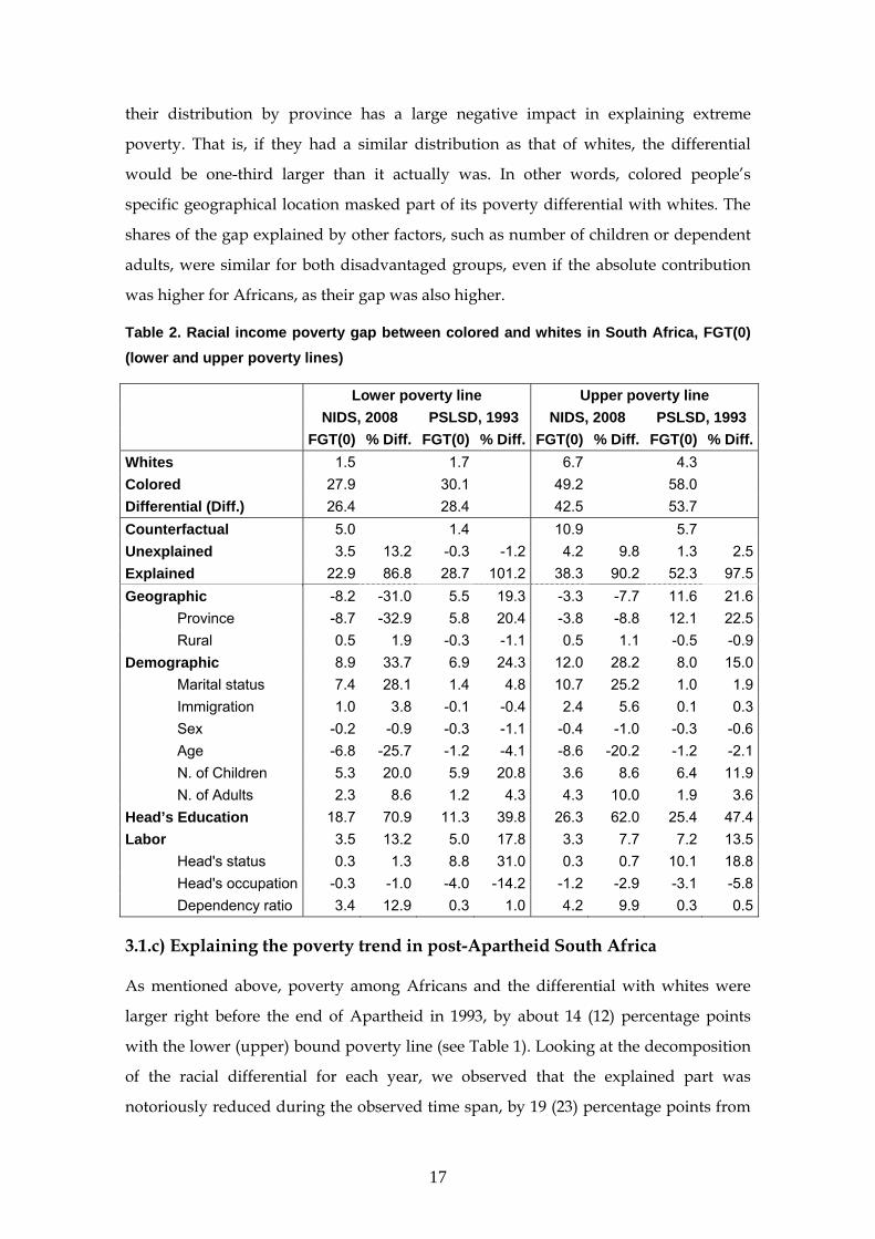
17

their distribution by province has a large negative impact in explaining extreme

poverty. That is, if they had a similar distribution as that of whites, the differential

would be one-third larger than it actually was. In other words, colored people’s

specific geographical location masked part of its poverty differential with whites. The

shares of the gap explained by other factors, such as number of children or dependent

adults, were similar for both disadvantaged groups, even if the absolute contribution

was higher for Africans, as their gap was also higher.

Table 2. Racial income poverty gap between colored and whites in South Africa, FGT(0)

(lower and upper poverty lines)

Lower poverty line Upper poverty line

NIDS, 2008 PSLSD, 1993 NIDS, 2008 PSLSD, 1993

FGT(0) % Diff. FGT(0) % Diff. FGT(0) % Diff. FGT(0) % Diff.

Whites 1.5 1.7 6.7 4.3

Colored 27.9 30.1 49.2 58.0

Differential (Diff.) 26.4 28.4 42.5 53.7

Counterfactual 5.0 1.4 10.9 5.7

Unexplained 3.5 13.2 -0.3 -1.2 4.2 9.8 1.3 2.5

Explained 22.9 86.8 28.7 101.2 38.3 90.2 52.3 97.5

Geographic -8.2 -31.0 5.5 19.3 -3.3 -7.7 11.6 21.6

Province -8.7 -32.9 5.8 20.4 -3.8 -8.8 12.1 22.5

Rural 0.5 1.9 -0.3 -1.1 0.5 1.1 -0.5 -0.9

Demographic 8.9 33.7 6.9 24.3 12.0 28.2 8.0 15.0

Marital status 7.4 28.1 1.4 4.8 10.7 25.2 1.0 1.9

Immigration 1.0 3.8 -0.1 -0.4 2.4 5.6 0.1 0.3

Sex -0.2 -0.9 -0.3 -1.1 -0.4 -1.0 -0.3 -0.6

Age -6.8 -25.7 -1.2 -4.1 -8.6 -20.2 -1.2 -2.1

N. of Children 5.3 20.0 5.9 20.8 3.6 8.6 6.4 11.9

N. of Adults 2.3 8.6 1.2 4.3 4.3 10.0 1.9 3.6

Head’s Education 18.7 70.9 11.3 39.8 26.3 62.0 25.4 47.4

Labor 3.5 13.2 5.0 17.8 3.3 7.7 7.2 13.5

Head's status 0.3 1.3 8.8 31.0 0.3 0.7 10.1 18.8

Head's occupation -0.3 -1.0 -4.0 -14.2 -1.2 -2.9 -3.1 -5.8

Dependency ratio 3.4 12.9 0.3 1.0 4.2 9.9 0.3 0.5

3.1.c) Explaining the poverty trend in post-Apartheid South Africa

As mentioned above, poverty among Africans and the differential with whites were

larger right before the end of Apartheid in 1993, by about 14 (12) percentage points

with the lower (upper) bound poverty line (see Table 1). Looking at the decomposition

of the racial differential for each year, we observed that the explained part was

notoriously reduced during the observed time span, by 19 (23) percentage points from

18

67 (74) to 48 (51). In contrast, the unexplained or conditional differential in poverty

rates increased from 2.5 (8) to 8 (19) percentage points. This suggests that the reduction

of poverty among Africans between 1993 and 2008 was driven by substantial progress

in their relevant characteristics, thus catching them up with whites. But this reduction

was not larger due to the opposite effect of these characteristics becoming less

protective in terms of keeping Africans out of poverty, as compared with whites.

More specifically, this convergence process involved two main factors: years of

schooling and the head of household’s occupation. The contribution of education to

higher poverty rates among Africans was virtually halved from 31 to 16 percentage

points with the lower bound, thus being able to explain by itself the whole observed

reduction in the poverty rate differential. The reduction in the racial poverty gap

associated with education in the case of the upper bound was more limited, from 36 to

25 percentage points, but still able to explain the entire reduction. Indeed, African

heads of household increased their years of education from 4.5 to 6.7 (as compared to

the increase among whites from 11.9 to 12.7). Similarly, the head of household’s

occupation played a fundamental role in 1993, contributing significantly to the racial

poverty differential that year, even after controlling for education and location (of 18

and 22.5 percentage points). This role vanished completely in 2008.23 The contribution

of demographic factors to higher poverty rates was barely similar in both years, while

the contribution of the higher concentration of Africans in rural areas substantially

increased between 1993 and 2008 (the share of rural population decreased more clearly

for whites, from 8.5 percent to 2.9, as compared to the relatively smaller reduction from

66.7 to 61.9 among Africans).24 Similar results can be found using the FGT(1) and

FGT(2) indices, with an even stronger contribution of increasing educational

attainment among Africans to reducing the racial poverty gap between 1993 and 2008

(see Table A3 in the Appendix).

23 The change in occupational classification makes the comparison difficult. However, in 1993, the sum of managerial, professional, and technical occupations accounted for 12 percent of the employed African heads of household (40 percent for whites), as compared to only 7 percent in the closest occupations in 1993 (48 percent of whites). 24 Obviously, ascertaining which factors changed their impact the most (detailed coefficients effect) would be quite interesting, as we have done with the characteristics effect. However, the disaggregation of the coefficients effect involves additional technical difficulties. There is no clear procedure to do it with our methodology. It could be done following, for example, Yun’s (2004) approach consisting of estimating poverty regressions for both groups; yet the small number of poor whites observed, especially in the NIDS dataset, discouraged us from doing so.

19

The results for colored people (Table 2) also showed a reduction in the differential in

poverty rates with respect to whites after Apartheid ended, especially in moderate

poverty, 2 (14) percentage points for the lower (upper) bound. But the latter reduction

was driven by a lower contribution of the province of residence.25 The conditional

racial poverty gap also increased, as for Africans, by about 3-4 percentage points.

3.2 Expenditure Poverty

How much of the previous results depend on the choice of income as the measure of

well-being? The risk of expenditure poverty for both whites and Africans was higher,

as compared with income poverty, and so was the differential, 61 (77) percentage

points with the lower (upper) poverty line. Thus, expenditure poverty for Africans was

about 25 times higher than for whites. The percentage of poverty in 2008 that was

explained by characteristics was similar to that of income and expenditure, but the

reasons differed. The main difference in using expenditure instead of income was the

much more important role played by education in explaining the differential in

poverty rates with the lower bound poverty line (25 percentage points, or 41 percent of

the gap). This is because the educational level attained by the head of household was

larger for those Africans identified as suffering from severe poverty with income but

not with expenditure (7.7 years on average) than for those in the reverse situation (5.9

years).26 Thus, the association between Africans’ higher severe poverty and lower

educational level was stronger when using expenditure rather than income.

The decline in expenditure poverty incidence for Africans between 1993 and 2008 was

more limited, as compared to that of income, especially for severe poverty (lower

bound) - from 68 to 64 percent of the population- but also for the upper bound poverty

line - from 88 to 80 percent. Thus, the reduction in the differential in poverty rates was

smaller with expenditure, or 6 (9) percentage points with the lower (upper) bound

poverty line. As in the case of income, this was due to a reduction in the explained

poverty gaps - 10 (25) percentage points- that was partially compensated for by an

increase in the unexplained part - from 3 to 7 (from 9 to 25) percentage points. The

impact of more years of schooling among Africans in reducing these differentials was

25 Given the change in provincial organization, this should be viewed with caution. 26 About 49 (28.5) percent of Africans in 2008 were identified as poor (non-poor) by both indicators using the lower poverty line. Thus, about 22.5 percent of Africans were classified as poor with only one indicator (14.5 percent with expenditure and 7.9 with income).

20

more limited than in the case of income: 4 (10) percentage points. In fact, in the case of

expenditure, labor market attachment (mainly due to the head of household’s

occupation) turned out to be much more important in explaining the reduction in

poverty, 8.5 (13) percentage points.

Table 3. Racial expenditure poverty gap between Africans and whites in South Africa,

FGT(0) (lower and upper poverty lines)

Lower poverty line Upper poverty line

NIDS, 2008 PSLSD, 1993 NIDS, 2008 PSLSD, 1993

FGT(0) % Diff. FGT(0) % Diff. FGT(0) % Diff. FGT(0) % Diff.

Whites 2.5 0.4 3.4 2.0

Africans 63.6 67.9 80.1 87.7

Differential (Diff.) 61.1 67.4 76.6 85.7

Counterfactual 9.6 3.3 28.6 11.4

Unexplained 7.1 11.6 2.9 4.3 25.2 32.8 9.3 10.9

Explained 54.1 88.4 64.5 95.7 51.5 67.2 76.3 89.1

Geographic 12.5 20.4 10.8 16.0 10.9 14.3 8.6 10.1

Province -1.2 -2.0 6.5 10.7 -2.6 -3.4 6.0 7.9

Rural 13.7 22.4 5.9 9.7 13.5 17.6 4.9 6.4

Demographic 13.9 22.7 13.5 20.0 10.1 13.1 13.7 16.0

Marital status 2.2 3.6 1.0 1.7 2.7 3.5 1.0 1.2

Immigration -1.3 -2.2 0.9 1.4 -1.5 -2.0 0.5 0.7

Sex 1.0 1.6 -0.5 -0.8 1.5 2.0 -0.4 -0.5

Age -2.8 -4.6 -1.5 -2.5 -4.7 -6.2 -1.1 -1.4

N. of Children 9.7 15.8 9.6 15.7 7.6 9.9 6.6 8.6

N. of Adults 5.2 8.5 4.4 7.3 4.5 5.9 3.5 4.5

Head’s Education 25.1 41.1 29.1 43.1 27.7 36.1 37.7 44.0

Labor 2.6 4.2 11.1 16.5 2.8 3.6 16.4 19.1

Head's status -1.4 -2.3 -1.4 -2.4 -2.5 -3.3 -1.1 -1.4

Head's occupation -1.1 -1.7 3.4 5.5 -0.7 -0.9 3.2 4.2

Dependency ratio 5.0 8.2 0.7 1.1 6.0 7.9 0.6 0.8

3.3 The role of family background

A person’s growing up in a poor family generally increases the chances that he or she

will experience poverty during adulthood through different channels (i.e., Hoelscher

2004; Magnuson and Votruba-Drzal 2009). For example, low parental investment or

financial stress may, later in life, increase poor children’s bad social behavior and

reduce their academic achievement. This is an important issue given the segregative

regime that dominated South Africa for so long and the low intergenerational mobility

that can be expected from that situation. Obviously, some current characteristics, such

21

as education, will be correlated with family background, thus capturing part of the

effect of the latter factor on the differential in poverty by race. But still, two households

with similar current observed characteristics could have different economic outcomes

on the basis of their families’ having different economic backgrounds. This would in

turn increase the explained poverty differential. Subsequently, ignoring past

inequalities could lead to an underestimation of the proportion of the racial differential

in poverty that is explained, as well as to an overestimation of the contribution of some

current characteristics. The larger the proportion of the poverty differential explained

by past inequalities, the slower the expected reduction in this differential because the

reduction will be mainly driven by convergence in current characteristics, as illustrated

by what happened after Apartheid. That is, not accounting for this factor could result

in a naïve or overly optimistic view of by how much improving Africans’ situation

would reduce poverty differentials.

To explore the role of past inequalities, we included as an additional potential factor

explaining poverty differentials by race a set of variables accounting for family

background available in NIDS (but not in PSLSD), such as occupation and years of

education of household head’s parents.27 As shown in Table 4, after taking into account

past inequalities, i) the whole set of worker characteristics now explained 90 percent or

more of the racial poverty gap; ii) family background turned out to be one of the main

explicative factors; iii) the contribution of other factors, especially the head of

household’s years of schooling, dropped; and iv) the role played by family background

was more relevant in explaining moderate than severe poverty and expenditure rather

than income poverty.

Indeed, the whole set of worker characteristics explained around 93 (94) percent of the

gap in income poverty incidence using the lower (upper) bound poverty lines.

Additionally, family background accounted for 11 (20) percentage points of the gap in

poverty rates, representing 19 (28) percent of that differential. Thus, past inequalities

had similar relevance to that of the other main factors, such as the head of household’s

years of schooling - 21 (26) percent of the gap-, number of children – 19 (17) percent-,

and living in rural areas - 20 (16) percent-, and their contributions shrunk.

Consequently, the main difference in explaining racial differentials for moderate as

27 These variables contain a large number of missing observations. For this reason, a category accounting for them was included in each case.

22

opposed to severe income poverty was the larger contribution of family background

and, to a lesser extent, the head of household’s education.

In the case of expenditure, worker characteristics explained 98 (90) percent of the racial

gap in poverty rates using the lower (upper) threshold, and family background on its

own explained 28 (31) percent, as compared to education, which accounted for 29 (28)

percent, way above living in rural areas, 19 (15) percent, or number of children, 18

(11.5) percent.

Table 4. Racial (income and expenditure) poverty gap between Africans and whites in

South Africa with family background, FGT(0) (lower and upper poverty lines)

Africans Colored

Income Expenditure Income Expenditure

Lower Upper Lower Upper Lower Upper Lower Upper

Counterfactual FGT(0) 5.3 11.0 3.7 11.4 0.1 0.3 0.1 0.2

Unexplained differential (%) 7.0 6.2 2.0 10.4 -5.3 -15.1 -7.7 -6.5

Explained differential (%) 93.0 93.8 98.0 89.6 105.3 115.1 107.7 106.5

Geographic 24.6 16.4 20.3 15.7 -24.9 -9.4 -14.7 -3.7

Province 4.9 0.4 1.0 0.5 -21.6 -7.1 -11.8 -1.5

Rural 19.7 16.1 19.3 15.2 -3.3 -2.3 -2.8 -2.2

Demographic 23.2 18.2 19.6 12.4 31.9 25.9 23.4 19.8

Marital status 5.3 5.0 3.6 4.6 11.4 10.4 7.1 6.4

Immigration -4.7 -6.0 -4.2 -4.7 1.9 2.1 -0.4 3.2

Sex 3.2 3.1 2.5 2.3 0.3 0.4 0.1 0.4

Age -4.0 -5.7 -6.0 -5.4 -1.9 -7.4 -9.0 -5.6

N. of Children 19.4 16.8 17.7 11.5 17.0 13.7 17.0 9.2

N. of Adults 4.1 5.1 6.0 4.1 3.2 6.7 8.6 6.2

Head’s Education 20.8 26.4 28.8 28.4 35.5 32.8 37.5 30.2

Labor 5.2 4.4 1.7 1.7 6.0 3.4 1.7 1.5

Head's status -7.0 -7.7 -4.6 -6.7 -2.4 -2.9 -3.9 -1.9

Head's occupation -0.4 0.6 0.2 1.3 0.5 -0.5 -0.7 -0.2

Dependency ratio 12.5 11.6 6.0 7.1 8.0 6.8 6.4 3.6

Family background 19.2 28.3 27.6 31.4 56.7 62.5 59.7 58.7

The percentage of the racial gap in income poverty explained by characteristics was

about 96 (93) percent when using FGT(2), with family background contributing 16 (20)

percent to the gap. Education played a similar role, explaining 18 (21) percent (see

Table A4 in the Appendix). In the case of expenditure, characteristics explained 99 (97)

percent of the gap in the case of FGT(2).

23

Family background was even more relevant in relative terms for colored people,

because it explained 57 (62) percent of the racial gap in income poverty incidence. It

was, in fact, the main explicative factor for this group, and its inclusion made the

overall gap being explained account for more than 100 percent, indicating that poverty

for this group would virtually vanish if they had the same characteristics as whites,

including family background. The head of household’s educational level and

demographic structure both explained another 35.5 (33) and 32 (26) percent,

respectively.

3.4 Deprivation

Finally, we took into account the growing consensus stressing that the experience of

poverty transcends financial poverty. That is, we adopted a more multidimensional

perspective. We measured the racial gap in material deprivation with regard to

different aspects, including needs insufficiently met, lack of appliances, and lack of

access to basic services. Table 5 presents the results. First, we measured the percentage

of individuals in each racial group that were deprived with respect to each single

attribute. In all cases, Africans were deprived in a much higher proportion than whites,

with the largest differentials (60 percentage points or more) found in the lack of

appliances (e.g., washing machine, motor vehicle, microwave, and/or computer) and

the lack of access to basic services (such as piped water or flush toilets).

Household characteristics explained a large share of this racial gap in cases where the

population lacked access to basic services, such as rubbish collection (99 percent) or

flush toilets (84 percent); lacked an electric or gas stove (92 percent); or received

inadequate healthcare (89 percent) and food (82 percent). However, in other cases,

characteristics explained less than half of the racial gap in deprivation, such as lacking

access to a cell (53 percent) or landline (27 percent) phone, a computer (36 percent), or a

washing machine (41 percent).

24

Table 5. Racial gap between Africans and whites in indicators of material deprivation in

South Africa, NIDS, 2008

Single indicator Africans whites differential counterf. % differential explained by

all geog. demog. educ. labor

Access to

formal dwelling 30.5 0.5 30.1 9.1 71.4 33.6 10.1 28.4 -0.7

piped water 66.8 5.5 61.4 75.8 69.5 44.9 2.9 23.1 -1.4

flush toilet 58.6 0.6 58.0 89.9 83.8 60.1 4.5 22.4 -3.3

electricity 23.2 1.4 21.8 93.3 75.7 50.7 -2.9 31.0 -3.1

landline telephone 94.0 49.0 45.0 18.3 27.3 11.6 6.3 6.1 3.3

cellphone 11.6 4.7 6.9 92.1 53.1 -60.9 -29.6 126.2 17.4

rubbish collection 55.0 4.3 50.7 95.0 98.6 73.8 1.3 24.8 -1.3

street lighting 66.6 11.9 54.7 71.7 70.1 55.1 0.6 17.7 -3.3

Insufficient needs

Food 42.8 10.2 32.7 16.2 81.6 11.5 24.3 46.3 -0.6

Housing 42.9 10.9 32.0 21.1 68.0 10.1 12.2 35.7 10.0

Clothing 44.5 18.1 26.4 28.1 62.1 6.6 9.7 38.3 7.6

healthcare 44.6 19.4 25.2 22.2 88.7 16.1 30.7 39.3 2.7

schooling 32.9 5.6 27.3 11.2 79.6 12.6 29.7 35.7 1.5

Ownership

radio 32.4 17.6 14.7 75.2 51.0 -19.3 27.0 43.2 0.2

TV 34.4 7.0 27.4 80.5 54.5 27.8 -5.0 32.4 -0.7

VCR/DVD 71.5 16.8 54.6 66.3 69.2 26.0 2.6 37.3 3.4

computer 93.6 33.9 59.7 28.0 36.3 6.2 3.6 22.4 4.0

electric/gas stove 36.1 9.8 26.3 88.1 92.0 45.1 -2.0 50.3 -1.4

microwave 72.7 14.3 58.4 68.1 69.9 30.1 5.5 31.7 2.6

fridge/freezer 46.5 5.6 40.9 84.2 75.0 31.5 4.5 35.2 3.8

washing machine 85.1 10.1 75.0 45.5 40.8 15.8 4.0 18.0 2.9

motor vehicle 88.1 18.7 69.4 45.7 48.7 9.3 8.0 25.2 6.2

Composite indicator

average 0.58 0.13 0.45 0.30 62.8 28.4 5.6 27.0 1.8

p99 50.4 1.0 49.4 8.1 85.4 47.6 3.5 35.6 -1.2

p95 74.4 5.0 69.4 22.3 74.9 32.8 8.0 31.3 2.8

p90 87.5 10.0 77.5 45.7 53.5 18.4 6.5 25.2 3.3

p75 94.6 25.0 69.6 65.1 42.1 13.9 4.9 17.9 5.5

p50 98.6 50.0 48.6 86.9 23.9 3.0 7.9 11.6 1.5

The main factors explaining these deprivations varied in each case. Unequal

geographical distribution is associated to a larger extent with deprivation in terms of

access to basic services, such as rubbish collection (74 percent), flush toilets (60

percent), street lighting (55 percent), or piped water (45 percent), as well as lacking

appliances, such as an electric/gas stove (45 percent). Education appeared responsible

to a larger extent for insufficient provision of food (46 percent), healthcare (39 percent),

25

clothing (38 percent), and schooling and housing (36 percent), as well as for access to a

cell phone (126 percent) or an electric/gas stove (50 percent) and a radio (43 percent).

Family demographics were also relevant, to a lesser extent than education, for

insufficient healthcare (31 percent), schooling (30 percent), and food (24 percent) and

the lack of a radio (27 percent). Labor-related factors were relevant only in explaining

the lack of a cell phone (17 percent), as well as sufficient housing (10 percent) and

clothing (8 percent).

As a second step, we constructed for each individual a composite indicator defined as

the weighted average of deprivation in each attribute, with weights estimated using

MCA, as described in the previous section. This indicator measured the degree of

accumulation of different forms of deprivation in the same individuals, accounting for

86 percent of the variability (principal inertia) of the original variables.28 The last six

rows of Table 5 display these results, jointly with the average of the indicator.

On average, deprivation among Africans was 58 percent of the maximum level

(deprived in all attributes), as compared to 13 percent in the case of whites. To compare

the distribution of this indicator for Africans and whites, we computed the percentage

of Africans with a level of deprivation higher than that for whites at different

percentiles of the whites’ distribution.29 Half of the African population experienced

deprivation above the 99th white percentile (as compared to 1 percent of whites, by

design), and this proportion increased to 74 percent at the 95th percentile, reaching 99

percent at the median of the whites’ distribution. The higher deprivation of Africans at

the 99th percentile could mostly (85 percent) be attributed to their household

characteristics, but this share decreased sharply as we moved from more severe to

more moderate deprivation (that is, from more to less accumulation of deprivation): 75

percent (95th), …, 24 percent (50th). Therefore, only severe deprivation was explained by

the unequal distribution of characteristics by race. The share explained for the 99th

28 The remaining 14 percent is accounted for by other three residual dimensions, not used for constructing the index, which are orthogonal with the main one, primarily explaining some rare profiles. The (negative) correlation of the individual composite indicator or deprivation with income and expenditure is of 47 and 50 percent, respectively. 29 Table A5 in the Appendix reports basic information about the MCA. The square correlation of dummy categories with the indicator was on average 0.85, with the largest values (above 0.95) for formal dwelling, DVD, and microwave and the lowest values (between 0.6 and 0.7) for needs met insufficiently. The largest contribution was then made by the lack of a washing machine, microwave, vehicle, computer, or DVD or piped water (between 0.040-0.055), and the lowest by the lack of a cellular phone or radio (0.001-0.005).

26

(95th) percentile is in fact similar to the case of the lower (upper) bound financial

poverty threshold. The main difference between material deprivation and poverty

came, however, from the main contributors to the racial gap. The geographical factors

turned out to be much more relevant in explaining extreme material deprivation than

in the case of poverty, 48 (33) percent of the gap for the 99th (95th) percentile. The

predominance of geographical factors for the deepest deprivation is related to the

previous results in which this factor was shown to be crucial in gaining access to basic

services. The contribution of this factor decreased sharply for lower percentiles (3

percent at the median). The second most important factor in explaining the gap in

extreme deprivation levels by race was the head of household’s educational level,

which explained 36 percent of the gap at the 99th percentile. Its relevance also

decreased with lower levels of deprivation, but less sharply than that of location: The

contribution of both factors was similar for the 95th percentile, but the head of

household’s educational level became the main factor for lower percentiles. The results

for the average deprivation showed that 63 percent of the racial gap was explained by

characteristics, namely geographical and educational factors, in a similar proportion

(28 and 27 percent), but this masked the different role that these factors played at

different levels of the distribution of deprivation discussed above.

The inclusion of family background as an explicative factor had a similar effect in

deprivation as with poverty (see Table 6). First, it substantially increased the

percentage of the gap explained by characteristics by reducing the effect of

unobservables. Deprivation in most attributes was explained by characteristics by 75

percent or more with few exceptions (only about 30 percent for lack of landline phone

and computer and about 70 percent for lack of radio and washing machine). Second,

family background turned out to be a factor as relevant as education and geographical

location, explaining between 20 and 40 percent of the gap in most cases (except for the

10 percent explained by lack of a landline phone and computer and the 100 percent

explained by the lack of a cellphone). Third, the proportion explained by the other two

main factors were generally reduced but with the same qualitative relevance as before.

27

Table 6. Racial gap between Africans and whites in deprivation indicators in South Africa with family

background, NIDS, 2008

Single indicator counterfactual % differential explained by

all geographic demographic education labor family background

Access to

formal dwelling 5.0 84.7 35.0 13.3 25.3 -7.5 18.7

piped water 81.2 78.2 40.3 3.2 18.8 -3.4 19.3

flush toilet 96.0 94.2 50.9 6.0 19.6 -5.0 22.6

electricity 96.2 89.1 41.5 1.5 25.8 -4.7 24.9

landline telephone 20.3 31.7 0.6 16.8 10.2 -6.3 10.4

cellphone 96.6 118.7 -23.3 -34.1 83.5 -8.3 100.8

rubbish collection 96.5 101.7 64.0 2.2 20.9 -6.0 20.6

street lighting 76.7 79.2 43.9 2.3 17.0 -3.4 19.4

Insufficient needs

food 9.4 102.4 16.5 19.5 40.3 -6.8 32.9

housing 13.4 92.3 16.2 15.4 30.4 0.3 30.0

clothing 14.9 112.0 17.0 17.3 37.6 -2.6 42.7

healthcare 18.2 104.7 19.7 20.7 32.3 -2.6 34.6

schooling 5.2 101.4 16.3 23.4 31.0 -0.9 31.7

Ownership

radio 78.1 71.3 -4.7 39.3 29.2 -12.1 19.6

TV 86.5 76.2 24.5 3.9 22.0 -2.2 28.1

VCR/DVD 77.2 89.0 21.1 5.7 28.9 3.5 29.9

computer 25.3 31.8 1.2 5.9 16.6 -5.1 13.1

electric/gas stove 91.8 106.4 37.6 1.4 37.4 0.2 29.8

microwave 74.9 81.6 26.0 6.6 24.2 -1.5 26.2

fridge/freezer 85.9 79.2 25.2 8.1 26.2 -0.5 20.2

washing machine 65.7 67.8 16.8 9.9 16.5 2.6 22.0

motor vehicle 63.9 74.9 11.7 12.8 21.2 6.3 23.0

Composite indicator

average 0.24 77.1 25.0 8.6 22.4 -1.8 22.9

p99 3.2 95.2 40.7 8.0 27.8 -5.3 24.0

p95 18.9 79.9 28.8 8.7 22.4 0.9 19.1

p90 28.2 75.8 19.7 8.8 21.0 2.0 24.3

p75 43.4 73.0 16.8 8.6 17.3 3.3 27.1

p50 84.2 29.6 -2.8 13.4 11.7 -5.5 12.8

Similar results were found in the case of the composite indicator. Considering that,

family background raised the share of the racial gap explained by characteristics on

average and at all percentiles. Characteristics generally explained most of the gap,

between 73 percent at the 75th percentile and 95 percent at the 99th (but still only 30

percent at the median). The qualitative roles of education and geographical location

discussed above was preserved but with smaller shares. Family background explained

28

23 percent of the gap in average deprivation, similar to the other two main factors. But

while the relevance of education and, especially, location still decreased for lower

levels of deprivation, family background had no clear distributional profile (its largest

share was at the 75th percentile and the lowest at the median). However, family

background became the most important factor for the intermediate percentiles, 90th and

75th.

4. Conclusions

Africans in South Africa face higher poverty and deprivation than whites. These racial

differentials are large even compared with those in other countries known for their

high racial inequalities, such as Brazil and the United States. In this paper, we have

investigated the extent to which the large racial poverty and deprivation differentials

in South Africa can be explained by inequalities in distribution characteristics across

races. To do so, we have estimated a counterfactual distribution in which Africans

were given the characteristics of whites.

Our results showed that the higher levels of Africans’ financial poverty and extreme

material deprivation could be almost fully explained by the accumulation of past and

present disadvantaged characteristics. We would underestimate the proportion of

these differentials if we did not control for family background among the

characteristics, which turned out to be a very relevant factor. Similarly, the role of

current characteristics, especially education, was significantly overestimated. The

effects of omitting past characteristics, such as occupation and years of schooling of

household head’s parents, were consistent with the fact that the reduction in the racial

poverty differential after Apartheid was smaller than would be expected from the

progress made by Africans in improving their characteristics so far, especially

educational level and labor market outcomes. The trend in the estimation of the racial

poverty differential, which cannot take family background into account, showed an

increase in the unexplained part partially compensating for the big reduction in the

explained differential, especially in income poverty. This inertia of past characteristics,

which can be attributed to the specific history of racial inequality in this country, could

burden future progress in reducing those racial gaps.

Regarding current characteristics, most of the poverty/deprivation differentials across

groups were associated with the overrepresentation of Africans in rural areas, their

29

households having more children and dependent adults, and the head of household’s

having a lower educational level. The head of household’s labor market status turned

out to have a much lower degree of association with those differentials in post-

Apartheid South Africa than previously. However, the role of each specific factor

varied depending on which measure of well-being was used and, often, on the severity

of poverty and deprivation being analyzed.

No factor took prominence in explaining the racial gap in poverty levels. Rather, the

accumulation of mainly pre-labor market disadvantages among Africans produced

higher poverty. Among the individual factors, educational level seemed the most

important with income and expenditure poverty, but in the case of income, educational

level was more important in explaining the differential in moderate than in severe

poverty. In contrast, the predominance of Africans in rural areas and the poorest

provinces was important in explaining poverty, but turned out to be the most

important factor in explaining Africans’ higher accumulation of deprivations,

especially lack of access to basic services. Other forms of deprivation, such as

insufficiently met needs, were more strongly associated, however, with lower

educational level among heads of household. The head of household’s educational

level replaced location as the main factor associated with higher deprivation rates

among Africans in more moderate forms of deprivation.

This studied further illustrated that gaps in poverty exist but are much lower for

colored people. They were explained primarily by family background, jointly with

educational level and family structure. In this case, educational level more clearly

served as a proxy for family background and was the most important factor if not

controlled for.

References

Agüero, J., M. R. Carter and J. Mayc (2007), “Poverty and Inequality in the First Decade of South Africa's Democracy: What can be Learnt from Panel Data from KwaZulu-Natal?”, Journal of African Economies, 16 (5): 782-812.

Argent, J., Finn, A., M. Leibbrandt, and I. Woolard (2009), “Poverty: Analysis of the NIDS Wave 1 Dataset”, NIDS Discussion Paper no. 13, South African Labour and Development Research Unit (SALDRU), School of Economics, University of Cape Town.

Asselin, L-M (2009), Analysis of Multidimensional Poverty: Theory and Case Studies, IDRC-CRDI and Springer, Economic Studies in Inequality, Social Exclusion and Well-Being, 7.

30

Bhorat, H., P. Naidoo and C. van der Westhuizen (2006), “Shifts in Non-income Welfare in South Africa, 1993-2004”, DPRU Conference Paper 18-20, October, Johannesburg.

Blinder, A. S. (1973), ‘‘Wage Discrimination: Reduced Form and Structural Estimates’’, Journal of Human Resources, 8(4): 436–55.

Cappellari, L. and S.P. Jenkins (2004), “Modeling Low Income Transitions”, Journal of Applied Econometrics, 19: 593–610.

Chantreuil, F. and A. Trannoy (1999), “Inequality Decomposition Values: the Trade-Off Between Marginality and Consistency”, THEMA Working Papers 99-24, THEMA, Université de Cergy-Pontoise.

Desai, M. and A. Shah (1988), “An Econometric Approach to the Measurement of Poverty”, Oxford Economic Papers, 40(3): 505-522.

DiNardo, J., N. M. Fortin, and T. Lemieux (1996), “Labor Market Institutions and the Distribution of Wages, 1973–1992: A Semiparametric Approach”, Econometrica 64:1001–1044.

Fairlie, R. W. (1999), “The Absence of the African-American Owned Business: An Analysis of the Dynamics of Self-employment”, Journal of Labor Economics, 17(1): 80-108.

Foster, J., J. Greer, and E. Thorbecke (1984), “A Class of Decomposable Poverty Measures”, Econometrica, 52: 761-765.

Gradín, C. (2009), “Why Is Poverty So High Among Afro-Brazilians? A Decomposition Analysis of the Racial Poverty Gap”, Journal of Development Studies, 45(9): 1-38.

Gradín, C. (2010), “Race and Income Distribution: Evidence from the US, Brazil and South Africa”, Ecineq Working Paper Series 2010-179.

Gradín, C. (2011), “Poverty Among Minorities in the United States: Explaining the Racial Poverty Gap for Blacks and Latinos”, forthcoming in Applied Economics.

Hoelscher, P. (2004), A Thematic Study using Transnational Comparisons to Analyse and Identify what Combination of Policy Responses are Most Successful in Preventing and Reducing High Levels of Child Poverty, Final report, European Commission, DG Employment and Social Affairs.

Hoogenveen, J., and B. Özler (2006), “Poverty and Inequality in Post-Apartheid South Africa: 1995- 2000”, in H. Bhorat, and R. Kanbur, Poverty and Policy in Post-Apartheid South Africa. Cape Town: HSRC Press.

Klasen, S. (2000), “Measuring Poverty and Deprivation in South Africa”, Review of Income and Wealth, 46(1): 33-58.

Leibbrandt, M., C. Woolard and I. Woolard (2009), “Poverty and Inequality Dynamics in South Africa: Post-Apartheid Developments in the Light of the Long-Run Legacy”, Chapter 10, in: Aron, J., B. Kahn and G. Kingdon (eds.), South African Economic Policy under Democracy, Oxford, Oxford University Press.

Leibbrandt, M., I. Woolard, A. Finn, and J. Argent (2010), “Trends in South African Income Distribution and Poverty Since the Fall of Apartheid”, OECD Social, Employment and Migration Working Papers No. 101.

Magnuson, K.A. and E. Votruba-Drzal (2009), “Enduring Influences of Childhood Poverty”, in S. Danziger and M. Cancian (Eds.), Changing Poverty, Changing Policies, New York, NY: Russell Sage.

May, J. (Editor) (2000), Poverty and Inequality in South Africa: Meeting the Challenge, David Phillip Publishers, Cape Town, and Zed Books, London-New York.

Meth, C. (2006), “What was the Poverty Headcount in 2004 and how does it Compare to Recent Estimates by van der Berg et al.?”, SALDRU Working Paper 01/2006, School of Economics, University of Cape Town.

31

Oaxaca, R. L. (1973), ‘‘Male-female Wage Differentials in Urban Labor Markets’’, International Economic Review, 14(3): 693–709.

Özler, B. (2007), “Not Separate, Not Equal: Poverty and Inequality in Post-Apartheid South Africa”, Economic Development and Cultural Change, vol. 55(3): 487-529.

Tsakloglou, P. and F. Papadopoulos (2002), “Poverty, Material Deprivation and Multi-dimensional Disadvantage During Four Life Stages: Evidence from the ECHP”, in M. Barnes, C. Heady, S. Middleton, J. Millar, F. Papadopoulos and P. Tsakloglou (eds) Poverty and Social Exclusion in Europe. Cheltenham: Edward Elgar.

Sastre, M. and A. Trannoy (2002), “Shapley Inequality Decomposition by Factor Components: Some Methodological Issues”, Journal of Economics 9: 51-89.

Seekings, J. (2007), “Poverty and Inequality after Apartheid”, Centre for Social Science Research, Working Paper No. 200, September, University of Cape Town.

Shorrocks, A. (1999), “Decomposition Procedures for Distributional Analysis: a Unified Framework Based on the Shapley Value”, Mimeo, University of Essex.

Statistics South Africa (2000), Measuring Poverty in South Africa, Pretoria: Statistics South Africa.

Van der Berg, S., M. Louw and D. Yu (2008), “Post-transition Poverty Trends Based on an Alternative Data Source”, South African Journal of Economics, 76(1): 58-76.

Van der Berg, S. and M. Louw (2004), “Changing Patterns of South African Income Distribution: Towards Time Series Estimates of Distribution and Poverty”, South African Journal of Economics, 72(3): 546-572.

Yun, M-S. (2004), “Decomposing Differences in the First moment”, Economics Letters, 82(2): 275-280.

32

Table A1 Regressors: average values and standard errors (s.e.) of continuous variables

Africans Whites Africans Whites

NIDS, 2008 mean (s.e) mean (s.e) PSLSD, 1993 mean (s.e) mean (s.e)

Western Cape 0.038 0.263 Cape 0.062 0.259

Eastern Cape 0.155 0.043 Transvaal (ref.) 0.205 0.553

Northern Cape 0.012 0.021 Orange F. S. 0.059 0.072

Free State/North West 0.224 0.106 rest of the country 0.675 0.116

Kwazulu Natal 0.149 0.089 rural area 0.667 0.085

Gaunteg (ref.) 0.208 0.342 n. of children 2.93 (2.27) 1.07 (1.17)

Mpumalanga 0.081 0.103 n. of adults 4.58 (2.51) 2.81 (1.22)

Limpopo 0.133 0.032 dependency ratio 0.64 (0.29) 0.32 (0.28)

rural area 0.619 0.029 Household head:

n. of children 2.23 (1.96) 0.76 (0.94) female 0.321 0.094

n. of adults 3.39 (2.10) 2.41 (0.95) age (missing) 0.031 0.002

dependency ratio 0.58 (0.33) 0.33 (0.30) 24 years old or less 0.013 0.030

Household head: 25-55 years old 0.563 0.795

Female 0.521 0.231 56+ years old 0.393 0.173

24 years old or less 0.053 0.034 spouse present (ref.) 0.592 0.860

25-55 years old (ref.) 0.642 0.654 deceased spouse 0.248 0.037

56+ years old 0.305 0.312 absent spouse 0.099 0.038

married (ref.) 0.408 0.721 no spouse 0.062 0.065

single with partner 0.104 0.034 5-years migrant 0.070 0.214

divorced/widow(er) 0.218 0.187 years of sch. (missing) 0.014 0.005

never married 0.270 0.058 years schooling 4.53 11.83

immigrant (missing) 0.056 0.078 labor status (missing) 0.174 0.015

non-immigrant (ref.) 0.719 0.491 Not Economically Active (ref.) 0.335 0.117

internal immigrant 0.197 0.343 discouraged unemployed 0.038 0.004

immigrant from abroad 0.028 0.088 strictly unemployed 0.022 0.012

5 years-migrant 0.135 0.294 formal employee 0.335 0.738

years of sch. (missing) 0.024 0.038 self-employed 0.063 0.100

years of schooling 6.50 12.27 casual employed 0.033 0.013

labor status (missing) 0.122 0.212 no occupation (or missing) (ref.) 0.633 0.238

Not Economically Active (ref.) 0.328 0.186 professional 0.026 0.240

discouraged unemployed 0.033 0.021 manager 0.005 0.165

strictly unemployed 0.092 0.028 clerical/sales 0.026 0.100

formal employee 0.305 0.405 transport 0.040 0.027

self-employed 0.075 0.125 service 0.061 0.044

casual employed 0.045 0.023 farming 0.033 0.008

no occupation (or missing) (ref.) 0.635 0.462 artisan 0.021 0.107

manager 0.012 0.092 foremen 0.012 0.040

professional 0.034 0.132 operator 0.039 0.025

technician 0.006 0.057 laborer 0.105 0.004

clerk 0.022 0.063

service worker 0.047 0.026

skilled farmer 0.021 0.005

craft trade worker 0.062 0.127

operator 0.047 0.023

elementary occupation 0.113 0.013

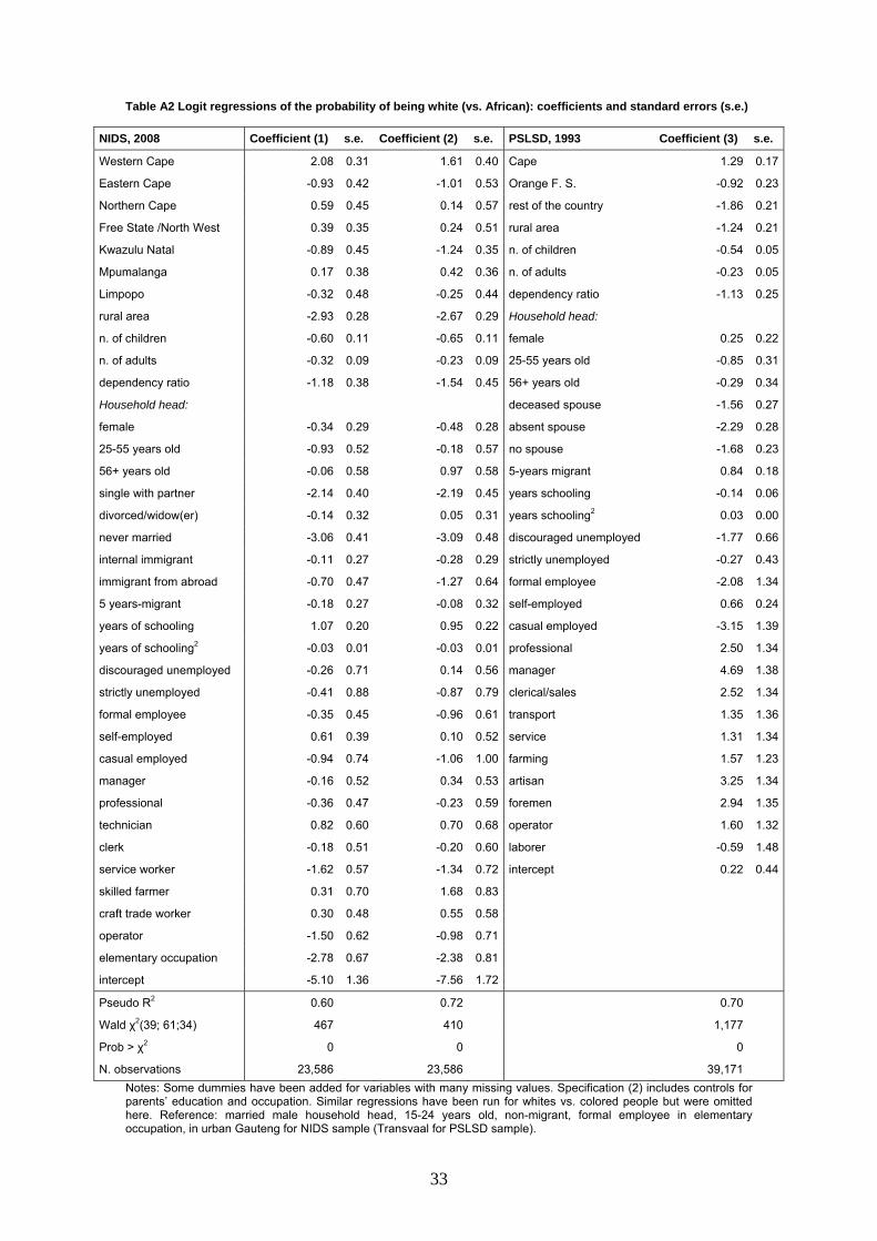
33

Table A2 Logit regressions of the probability of being white (vs. African): coefficients and standard errors (s.e.)

NIDS, 2008 Coefficient (1) s.e. Coefficient (2) s.e. PSLSD, 1993 Coefficient (3) s.e.

Western Cape 2.08 0.31 1.61 0.40 Cape 1.29 0.17

Eastern Cape -0.93 0.42 -1.01 0.53 Orange F. S. -0.92 0.23

Northern Cape 0.59 0.45 0.14 0.57 rest of the country -1.86 0.21

Free State /North West 0.39 0.35 0.24 0.51 rural area -1.24 0.21

Kwazulu Natal -0.89 0.45 -1.24 0.35 n. of children -0.54 0.05

Mpumalanga 0.17 0.38 0.42 0.36 n. of adults -0.23 0.05

Limpopo -0.32 0.48 -0.25 0.44 dependency ratio -1.13 0.25

rural area -2.93 0.28 -2.67 0.29 Household head:

n. of children -0.60 0.11 -0.65 0.11 female 0.25 0.22

n. of adults -0.32 0.09 -0.23 0.09 25-55 years old -0.85 0.31

dependency ratio -1.18 0.38 -1.54 0.45 56+ years old -0.29 0.34

Household head: deceased spouse -1.56 0.27

female -0.34 0.29 -0.48 0.28 absent spouse -2.29 0.28

25-55 years old -0.93 0.52 -0.18 0.57 no spouse -1.68 0.23

56+ years old -0.06 0.58 0.97 0.58 5-years migrant 0.84 0.18

single with partner -2.14 0.40 -2.19 0.45 years schooling -0.14 0.06

divorced/widow(er) -0.14 0.32 0.05 0.31 years schooling2 0.03 0.00

never married -3.06 0.41 -3.09 0.48 discouraged unemployed -1.77 0.66

internal immigrant -0.11 0.27 -0.28 0.29 strictly unemployed -0.27 0.43

immigrant from abroad -0.70 0.47 -1.27 0.64 formal employee -2.08 1.34

5 years-migrant -0.18 0.27 -0.08 0.32 self-employed 0.66 0.24

years of schooling 1.07 0.20 0.95 0.22 casual employed -3.15 1.39

years of schooling2 -0.03 0.01 -0.03 0.01 professional 2.50 1.34

discouraged unemployed -0.26 0.71 0.14 0.56 manager 4.69 1.38

strictly unemployed -0.41 0.88 -0.87 0.79 clerical/sales 2.52 1.34

formal employee -0.35 0.45 -0.96 0.61 transport 1.35 1.36

self-employed 0.61 0.39 0.10 0.52 service 1.31 1.34

casual employed -0.94 0.74 -1.06 1.00 farming 1.57 1.23

manager -0.16 0.52 0.34 0.53 artisan 3.25 1.34

professional -0.36 0.47 -0.23 0.59 foremen 2.94 1.35

technician 0.82 0.60 0.70 0.68 operator 1.60 1.32

clerk -0.18 0.51 -0.20 0.60 laborer -0.59 1.48

service worker -1.62 0.57 -1.34 0.72 intercept 0.22 0.44

skilled farmer 0.31 0.70 1.68 0.83

craft trade worker 0.30 0.48 0.55 0.58

operator -1.50 0.62 -0.98 0.71

elementary occupation -2.78 0.67 -2.38 0.81

intercept -5.10 1.36 -7.56 1.72

Pseudo R2 0.60 0.72 0.70

Wald χ2(39; 61;34) 467 410 1,177

Prob > χ2 0 0 0

N. observations 23,586 23,586 39,171

Notes: Some dummies have been added for variables with many missing values. Specification (2) includes controls for parents’ education and occupation. Similar regressions have been run for whites vs. colored people but were omitted here. Reference: married male household head, 15-24 years old, non-migrant, formal employee in elementary occupation, in urban Gauteng for NIDS sample (Transvaal for PSLSD sample).

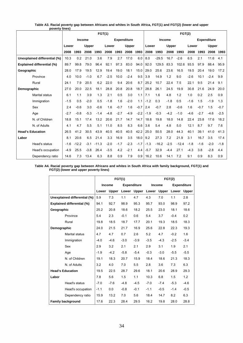
34

Table A3. Racial poverty gap between Africans and whites in South Africa, FGT(1) and FGT(2) (lower and upper poverty lines)

FGT(1) FGT(2)

Income Expenditure Income Expenditure

Lower Upper Lower Upper Lower Upper Lower Upper

2008 1993 2008 1993 2008 1993 2008 1993 2008 1993 2008 1993 2008 1993 2008 1993

Unexplained differential (%) 10.3 0.2 21.0 3.6 7.9 2.7 17.0 6.0 8.0 -29.5 16.7 -2.6 6.5 2.1 11.6 4.1

Explained differential (%) 89.7 99.8 79.0 96.4 92.1 97.3 83.0 94.0 92.0 129.5 83.3 102.6 93.5 97.9 88.4 95.9

Geographic 28.0 17.9 19.5 12.9 19.4 19.0 18.1 15.0 29.0 25.6 23.6 16.5 19.5 20.4 19.0 17.2

Province 4.0 10.0 -1.0 6.7 -2.5 10.0 -2.4 9.5 3.9 14.9 1.2 9.0 -2.6 10.1 -2.4 9.9

Rural 24.1 7.9 20.5 6.2 22.0 9.4 20.6 8.7 25.2 10.7 22.4 7.5 22.1 9.5 21.4 9.1

Demographic 27.0 20.0 22.5 18.1 28.8 20.8 20.8 18.7 28.8 26.1 24.5 19.9 30.8 21.6 24.9 20.0

Marital status 6.1 1.1 3.9 1.3 2.1 0.5 3.0 1.1 7.1 1.6 4.8 1.2 1.0 0.2 2.5 0.9

Immigration -1.5 0.5 -2.0 0.5 -1.8 1.6 -2.0 1.1 -1.2 0.3 -1.8 0.5 -1.6 1.5 -1.9 1.3

Sex 2.4 -0.6 3.0 -0.6 1.6 -0.7 1.6 -0.7 2.4 -0.7 2.8 -0.6 1.6 -0.7 1.5 -0.7

Age -2.7 -0.8 -5.3 -1.4 -4.8 -2.7 -4.9 -2.2 -1.9 -0.3 -4.2 -1.0 -4.6 -2.7 -4.6 -2.5

N. of Children 18.8 15.1 17.4 13.2 20.6 21.7 14.7 14.7 18.8 19.8 18.0 14.8 22.4 23.8 17.6 18.2

N. of Adults 4.1 4.7 5.5 5.1 11.0 8.5 8.3 6.6 3.6 5.4 4.8 5.0 12.1 8.7 9.7 7.6

Head’s Education 26.5 41.2 30.5 43.9 40.5 40.5 40.5 42.2 25.0 50.5 28.0 44.3 40.1 39.1 41.0 41.3

Labor 8.1 20.6 6.5 21.4 3.3 16.9 3.5 18.0 9.2 27.3 7.2 21.9 3.1 16.7 3.5 17.4

Head's status -1.6 -12.2 -3.1 -11.3 -2.0 -1.7 -2.3 -1.7 -1.3 -16.2 -2.5 -12.4 -1.8 -1.6 -2.0 -1.8

Head's occupation -4.9 25.5 -3.8 26.4 -3.5 4.2 -2.1 4.4 -5.7 32.9 -4.4 27.1 -4.3 3.8 -2.8 4.4

Dependency ratio 14.6 7.3 13.4 6.3 8.8 0.9 7.9 0.9 16.2 10.6 14.1 7.2 9.1 0.9 8.3 0.9

Table A4. Racial poverty gap between Africans and whites in South Africa with family background, FGT(1) and

FGT(2) (lower and upper poverty lines)

FGT(1) FGT(2)

Income Expenditure Income Expenditure

Lower Upper Lower Upper Lower Upper Lower Upper

Unexplained differential (%) 5.9 7.3 1.1 4.7 4.3 7.0 1.1 2.8

Explained differential (%) 94.1 92.7 98.9 95.3 95.7 93.0 98.9 97.2

Geographic 25.2 20.8 18.6 18.2 25.5 23.0 18.1 18.6

Province 5.4 2.3 -0.1 0.6 5.4 3.7 -0.4 0.2

Rural 19.8 18.5 18.7 17.7 20.1 19.3 18.5 18.3

Demographic 24.0 21.5 21.7 16.9 25.6 22.8 22.3 19.3

Marital status 4.7 4.7 0.7 2.6 5.2 4.7 -0.2 1.6

Immigration -4.0 -4.6 -3.0 -3.9 -3.5 -4.3 -2.5 -3.4

Sex 2.9 3.2 2.1 2.1 2.9 3.1 1.9 2.1

Age -1.9 -4.2 -5.8 -5.4 -0.3 -3.0 -5.5 -5.5

N. of Children 19.1 18.3 20.7 15.9 18.4 18.6 21.3 18.3

N. of Adults 3.2 4.0 7.0 5.5 2.8 3.6 7.3 6.3

Head’s Education 19.5 22.5 28.7 29.6 18.1 20.6 28.9 29.3

Labor 7.8 5.6 1.5 1.1 10.3 6.8 1.5 1.2

Head's status -7.0 -7.6 -4.8 -4.5 -7.0 -7.4 -5.3 -4.6

Head's occupation -1.1 0.0 -0.8 -0.1 -1.1 -0.5 -1.4 -0.5

Dependency ratio 15.9 13.2 7.0 5.6 18.4 14.7 8.2 6.3

Family background 17.6 22.3 28.4 29.5 16.2 19.8 28.0 28.8

35

Table A5. MCA: deprivation composite indicator of Africans and whites in South Africa

Burt/adjusted inertias

Dimension principal inertia

percent cumulative percent

dim 1 0.07608 86.33 86.33

dim 2 0.00500 5.67 92.00

dim 3 0.00064 0.72 92.72

dim 4 0.00054 0.61 93.33

Total 0.08812 100

(22,193 obs.)

Statistics for column categories in standard normalization

Categories coordinate

square correlation

contribution Categories coordinatesquare correlation

contribution

formal dwelling

no 0.586 0.966 0.011 healthcare no 0.611 0.639 0.01

yes -1.56 0.966 0.03 yes -0.849 0.639 0.014

piped water

no 1.513 0.928 0.041 schooling no 0.489 0.658 0.008

yes -0.997 0.928 0.027 yes -1.141 0.658 0.018

flush toilet

no 1.336 0.862 0.039 radio no 0.239 0.858 0.002

yes -1.211 0.862 0.035 yes -0.538 0.858 0.004

electricity no 0.509 0.895 0.009 TV no 0.704 0.914 0.015

yes -1.931 0.895 0.035 yes -1.533 0.914 0.034

landline telephone

no 2.678 0.936 0.035VCR/ DVD

no 1.6 0.959 0.04

yes -0.324 0.936 0.004 yes -0.837 0.959 0.021

cellphone no 0.119 0.86 0.001 computer no 2.75 0.919 0.044

yes -0.978 0.86 0.005 yes -0.401 0.919 0.006

rubbish collection

no 1.169 0.835 0.031electric/ gas stove

no 0.744 0.916 0.017

yes -1.189 0.835 0.032 yes -1.49 0.916 0.034

street lighting

no 1.245 0.85 0.028 microwave no 1.768 0.954 0.048

yes -0.803 0.85 0.018 yes -0.891 0.954 0.024

food no 0.676 0.681 0.013fridge/ freezer

no 0.959 0.929 0.024

yes -1.042 0.681 0.019 yes -1.319 0.929 0.033

housing no 0.675 0.66 0.013washing machine

no 2.306 0.928 0.055

yes -1.035 0.66 0.019 yes -0.684 0.928 0.016

clothing no 0.679 0.631 0.012motor vehicle

no 2.329 0.925 0.048

yes -0.951 0.631 0.017 yes -0.557 0.925 0.011