Economics 250a Racial Disparities and Discrimination Reading List Note: there is a huge literature on this topic in economics and in other social sciences. This lecture will focus on a few selected issues. The first four papers are review articles. The next two are key papers that have a large impact on current research. The last 3 are recent papers on race and crime. Joseph Altonji and Rebecca Blank. "Race and Gender in the Labor Market." In O. Ashenfelter and D. Card, Handbook of Labor Economics volume 3. Elsevier, 1999. This is good background material. Be aware that the tables are not very reliable! Kerwin Charles and Jonathan Guryan. "Studying Discrimination: Fundamental Challenges and Recent Progress." Annual Review of Economics 3 (2011): 479-511. Roland Fryer. "Racial Inequality in the 21st Century: The Declining Significance of Discrimination." In O. Ashenfelter and D. Card, Handbook of Labor Economics volume 4B. Elsevier, 2011. Lang, Kevin and Jee-Yeon Lehmann. "Racial Discrimination in the Labor Market: Theory and Empirics." Journal of Economics Literature 50 (2012): 959-1006. Coate, Stephen and Glenn Loury. "Will Affirmative Action Policies Eliminate Negative Stereotypes?" American Economic Review 82 (1993): 1220-1240. Marianne Bertrand and Sendhil Mullainathan. "Are Emily and Greg More Employable Than Lakisha and Jamal? A Field Experiment on Labor Market Discrimiation." American Economic Review 94 (2004): 991-1013. Anwar, Shamena, Patrick Bayer and Randi Hjalmarsson. "The Impact of Jury Race in Criminal Trials." Quarterly Journal of Economics (2014): 1-39. Roland Fryer, “An Empirical Analysis of Racial Differences in Police Use of Force”. Unpublished, June 2016. Steven Raphael and Sandra Rozo. “Racial Disparities in the Acquisition of Juvenile Arrest Records”. Unpublished October 2016.

Economics 250aRacial Disparities and Discrimination

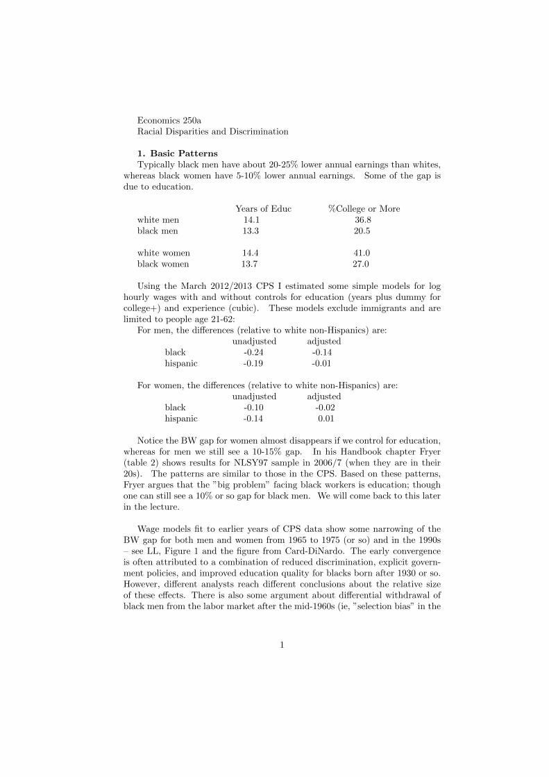
1. Basic PatternsTypically black men have about 20-25% lower annual earnings than whites,

whereas black women have 5-10% lower annual earnings. Some of the gap isdue to education.

Years of Educ %College or Morewhite men 14.1 36.8black men 13.3 20.5

white women 14.4 41.0black women 13.7 27.0

Using the March 2012/2013 CPS I estimated some simple models for loghourly wages with and without controls for education (years plus dummy forcollege+) and experience (cubic). These models exclude immigrants and arelimited to people age 21-62:

For men, the differences (relative to white non-Hispanics) are:unadjusted adjusted

black -0.24 -0.14hispanic -0.19 -0.01

For women, the differences (relative to white non-Hispanics) are:unadjusted adjusted

black -0.10 -0.02hispanic -0.14 0.01

Notice the BW gap for women almost disappears if we control for education,whereas for men we still see a 10-15% gap. In his Handbook chapter Fryer(table 2) shows results for NLSY97 sample in 2006/7 (when they are in their20s). The patterns are similar to those in the CPS. Based on these patterns,Fryer argues that the ”big problem” facing black workers is education; thoughone can still see a 10% or so gap for black men. We will come back to this laterin the lecture.

Wage models fit to earlier years of CPS data show some narrowing of theBW gap for both men and women from 1965 to 1975 (or so) and in the 1990s– see LL, Figure 1 and the figure from Card-DiNardo. The early convergenceis often attributed to a combination of reduced discrimination, explicit govern-ment policies, and improved education quality for blacks born after 1930 or so.However, different analysts reach different conclusions about the relative sizeof these effects. There is also some argument about differential withdrawal ofblack men from the labor market after the mid-1960s (ie, ”selection bias” in the

1

earnings of black men). Black women tend to have higher employment ratesthan white women so this is not a factor for them.

2. Models of Discrimination and Racial Gapsa. Becker’s modelThe ”classic” Becker model of discrimination is one in which employers face

horizontal supply curves of workers of both races, and have a distaste for hiringblack workers. Employer j maximizes an objective like:

f(La + Lb)− waLa − (wb + dj)Lb

where La and Lb are employment of whites and blacks, respectively, wa andwb are their market wages, and dj is the ”disrimination coefficient” of employerj. Note we have assumed B and W are equally productive. This firm acts asif black workes ”cost” wb + dj . So if dj > wa − wb this employer hires onlywhites, whereas if dj < wa − wb it hires only blacks.

In the market equilibrium, B’s are employed at all-black firms with the lowestlevels of dj . If total demand by firms with dj = 0 is less than the supply of B’sthen the black wage is forced down until the last B is hired. The market-widewage gap is determined by djm where jm is the most discriminatory firm thathires B’s: the ”marginal” hiring firm. Notice that this means that even at non-discriminating firms, B’s are paid their lower market wage (and are a bargain):so none of the infra-marginal all-black firms would be even interested in hiringa white worker.

The stark Becker model is obviously not a good one to take to the datafrom the last few decades. (The ideas were written up in the 1950s, when therewere many 100% segregated firms). Clearly, we rarely see any firms that hireonly B’s and (among larger employers in areas with reasonable numbers of B’s)very few that have hire only W’s. One “problem” for the Becker model is thatsince the 1960’s, firms cannot legally justify paying a lower wage to equallyproductive B and W workers by arguing that B’s have lower market wages. Ofcourse productivity is rarely observable so...

Nevertheless, Charles and Guryan (JPE, 2008) try to test this model bylooking at how the BW wage gap in a state varies with the strength of discrim-inatory preferences exhibited by whites in the bth percentile of the distributionof discriminatory preferences, where b is the share of black workers in the area.

b. Statistical DiscriminationIn the late 1960’s Arrow proposed a model of ”discrimination” based on

imperfect information. Let pi represent the true productivity of worker i andassume that among W’s, pi ∼ N(µa, σ

2a), whereas among B’s, pi ∼ N(µb, σ

2b ).

Suppose that employers don’t observe p perfectly but instead observe a noisyversion:

qi = pi + ηi

where ηi ∼ N(0, σ2η). If employers pay wages equal to expected productivity

then the wage for a B with observed productivity q will be:

wi = (1− λb)µb + λbqi

2

where λb = σ2b/(σ

2b + σ2

η), whereas the wage paid to a white worker with thesame observed productivity will be:

wi = (1− λa)µa + λaqi

where λa = σ2a/(σ

2a+σ2

η). In the simplest case where σ2a = σ2

b , the λ′s are equal,but if µb < µa a B worker will receive a lower wage than a W with the same q.

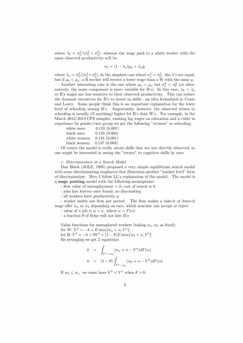
Another interesting case is the one where µb = µa but σ2a < σ2

b (or alter-natively, the noise component is more variable for B’s). In this case, λb < λaso B’s wages are less sensitive to their observed productivity. This can reducethe dynamic incentives for B’s to invest in skills - an idea formalized in Coateand Loury. Some people think this is an important explanation for the lowerlevel of schooling among B’s. Importantly, however, the observed return toschooling is usually (if anything) higher for B’s than W’s. For example, in theMarch 2012/2013 CPS samples, running log wages on education and a cubic inexperience by gender/race group we get the following ”returns” to schooling:

white men: 0.121 (0.001)black men: 0.123 (0.004)white women: 0.124 (0.001)black women: 0.137 (0.003)

Of course the model is really about skills that are not directly observed, soone might be interested in seeing the ”return” to cognitive skills by race.

c. Discrimination in a Search ModelDan Black (JOLE, 1995) proposed a very simple equilibrium search model

with some discriminating employers that illustrates another ”market level” formof discrimination. Here I follow LL’s explanation of the model. The model isa wage posting model with the following assumptions:

- flow value of unemployment = 0; cost of search is k- jobs last forever once found; no discounting- all workers have productivity p- worker meets one firm per period. The firm makes a take-it or leave-it

wage offer wa or wb depending on race, which searcher can accept or reject- value of a job is w + α where α ∼ F (α)- a fraction θ of firms will not hire B’s

Value functions for unemployed workers (taking wa, wb as fixed):for W: V a = −k + Emax{wa + α, V a}for B: V b = −k + θV b + (1− θ)Emax{wb + α, V b}Re-arranging we get 2 equations:

k =

ˆV a−wa

(wa + α− V a)dF (α)

k = (1− θ)ˆV b−wb

(wb + α− V b)dF (α)

If wb ≤ wa we must have V b < V a when θ > 0.

3

What do firms do? Firms have monopsonistic power and can offer a wagebelow p and take the chance that the worker has a high value of α. Since jobslast forever and there is no discounting the optimal strategy for a firm facedwith a white applicant is to maximize

πa = (1− F (V a − wa))(p− wa)

while for an unpredjudiced firm faced with a black applicant, the firm willmaximize

πb = (1− F (V b − wb))(p− wb)

The FOC’s imply:

p− wa =1− F (V a − wa)

f(V a − wa)= m(V a − wa)

p− wb =1− F (V b − wb)f(V b − wb)

= m(V b − wb)

Now assume that m() is strictly decreasing (Note m is the ”Mills ratio” andwill be decreasing if F is log-concave, a standard assumption in such problems).Then the solutions must have wb < wa.

The economic idea is that if some firms won’t hire B’s, then non-discriminatingfirms have more market power over B’s, and set a lower wage. Note that in thismodel (as in the Becker model) the presence of the discriminating firms conveysa benefit to non-discriminators

d. Rational Sterotype ModelsCoate and Loury develop a model with workers investing in skills (or not)

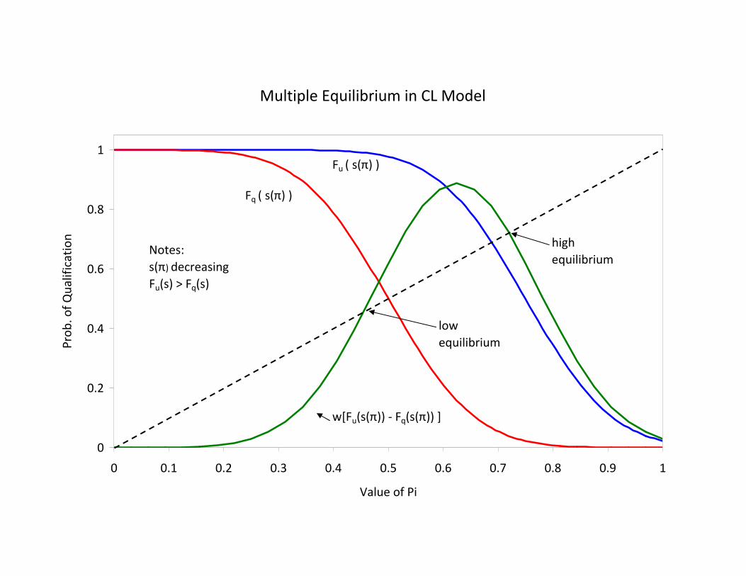
and firms partially observing productivity and deciding how to assign workers,in which there can be multiple equilibria.1 In a ”low” equilibrium, firms expecta low level of investment, and so require a very high signal in order to assignworkers to a high-productivity job. Given that high bar, most workers find itoptimal not to invest. In the ”high” equilibrium, firms expect a high level ofinvestment, and so have a relatively low threshold for the observed signal toassign workers to a high-productivity job. Given that lower bar, most workersfind it optimal to invest.

The following ”sketch” of their model is from LL.- workers are in one of 2 groups- workers have a cost of investment c ∼ U [0, 1]. Worker sees c and decides to

invest or not. Workers who invest are ”qualified” (q). Rest are unqualified (u).

1The possibility of multiple equilibrium plays a large role in the statistical discriminationliterature because the game is to think of models where (1) no one has direct animus againstB’s; (2) B’s and W’s are fundamentally the same; (3) everyone is rational; and yet (4) B’schoose lower levels of human capital investment and end up getting paid less. If this is truethan a “big push” could get us to a new equilibrium.

4

- firm sees group and a signal θ. CDF of the signal is Fq(θ) for qualified andFu(θ) for unqualified, with Fq(θ) < Fu(θ) – so low values of θ are more likelyfor U’s

- firm has 2 jobs: ”easy” (job 0) is appropriate for q or u. The ”hard” job(job 1) is only appropriate for q’s. Worker is paid a wage w if assigned to thehard job (and 0 if assigned to the easy job).

- firm has priors πa and πb that members of the 2 groups are qualified- firm will assign a worker with prior π to the high task if θ ≥ s∗(π), where

s∗ is a decreasing function (higher π means a lower standard). (See CL, equation1 and 2 for long derivation, based on posterior prob of being qualified, given θ,and payoff to firm of correct vs incorrect assignment).

- given standard s a worker who is qualified gets the hard job with probability(1 − Fq(s)), while if he were unqualified the probability is (1 − Fu(s)). So thebenefit of investing is w(Fu(s)− Fq(s)), and a worker with cost c will invest if

w[Fu(s)− Fq(s)] > c.

Notice that its as if a worker has only 1 chance to get hired for the better job.If c ∼ U [0, 1], then fraction who invest is

π∗ = w[Fu(s(π))− Fq(s(π))]

Since Fu(s) and Fq(s) are S-shaped functions with Fq(s) underneath, the rhs ofthis equation is increasing and then decreasing in s (i.e. inverse-U shaped).

In equilibrium we must have:

π = w[Fu(s∗(π))− Fq(s∗(π))]

This can have multiple solutions (see Figure at the end of lecture), so there canbe both High and Low equ.

3. Some Important Recent Papersa. Bertrand and Mullainathan – the ”names” paperThis is a carefully designed audit study that has inspired many later studies

on lots of different issues using a similar design. (BM were not the first to sendrandomized applications but they did a very good job and had a lot of powerint their design).

The paper is important because it seems to establish with a strong researchdesign that blacks and whites are NOT treated equally by firms. Nevertheless,some authors have tried to argue that BM’s use of black names as a signifier ofrace is confounded by the fact that black names also signify “low SES”.

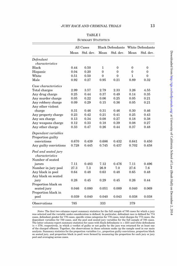
c) Three Recent crime papersAnwar, Bayer and Hjalmarsson (QJE, 2012) - the ”black jury” paper.Fryer’s “Use of Force” paperRaphael and Rozo’s “Juvenile arrest” paper Black men are disproportion-

5

Multiple Equilibrium in CL Model

0

0.2

0.4

0.6

0.8

1

0 0.1 0.2 0.3 0.4 0.5 0.6 0.7 0.8 0.9 1

Value of Pi

Prob

. of Q

ualif

icat

ion

lowequilibrium

highequilibrium

Fu ( s(π) )

Fq ( s(π) )

Notes:s(π) decreasingFu(s) > Fq(s)

w[Fu(s(π)) - Fq(s(π)) ]

ately involved in criminal justice (arrests, incarcerations, etc), and there is aconcern that this factor hurts their labor market outcomes, especially with theready availability of information about past criminal records.

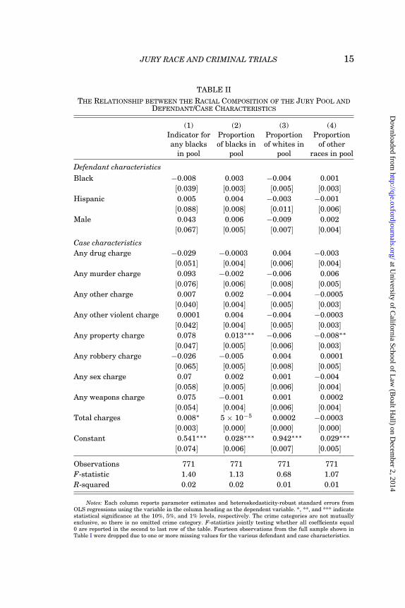
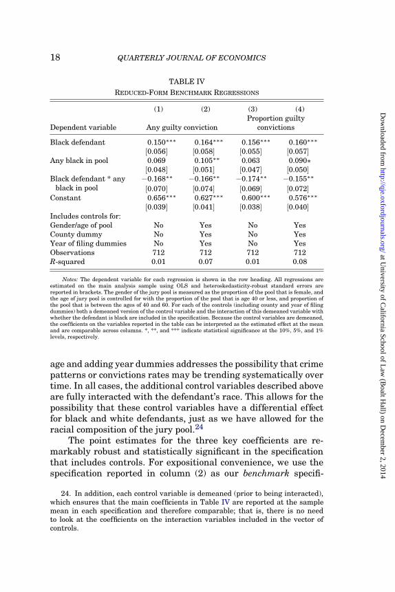
ABH is a carefully designed jury study that shows that when there are moreblacks in a jury, a black defendent is less likely to be convicted. The instrumentis the presence of any black in the jury pool, which they show seems to passstandard exogeneity/design tests. The paper is one of several out there nowwhich show that black defendents are treated differently.

Fryer’s “use of force” paper uses data from several sources – including theNYC stop and frisk program – to examine the probability of a police use of force,conditional on an interaction. He finds that P(use of force|stop) is higherfor blacks and hispanics in NYC. Interestingly, he does not find that blacks orHispanics are more likely to be found with a weapon, conditional on the levelof force.

6

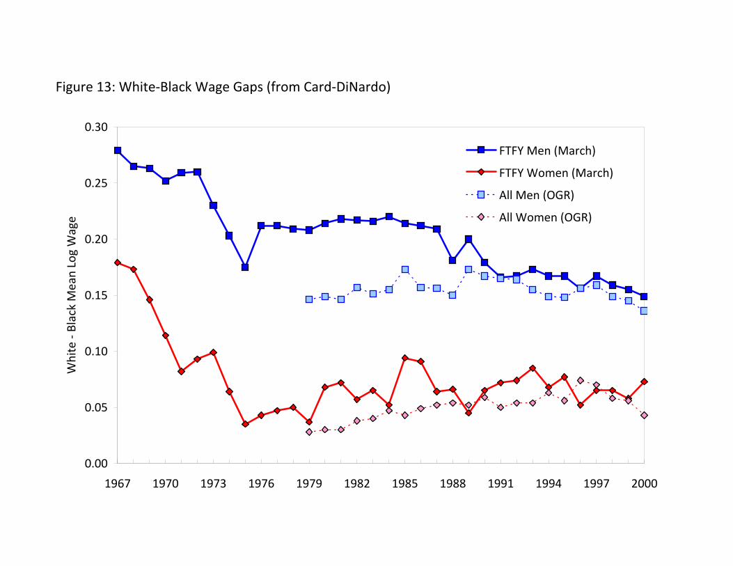
Figure 13: White‐Black Wage Gaps (from Card‐DiNardo)

0.00

0.05

0.10

0.15

0.20

0.25

0.30

1967 1970 1973 1976 1979 1982 1985 1988 1991 1994 1997 2000

White ‐ Black Mean Log Wage

FTFY Men (March)

FTFY Women (March)

All Men (OGR)

All Women (OGR)

Journal of Economic Literature, Vol. L (December 2012)964

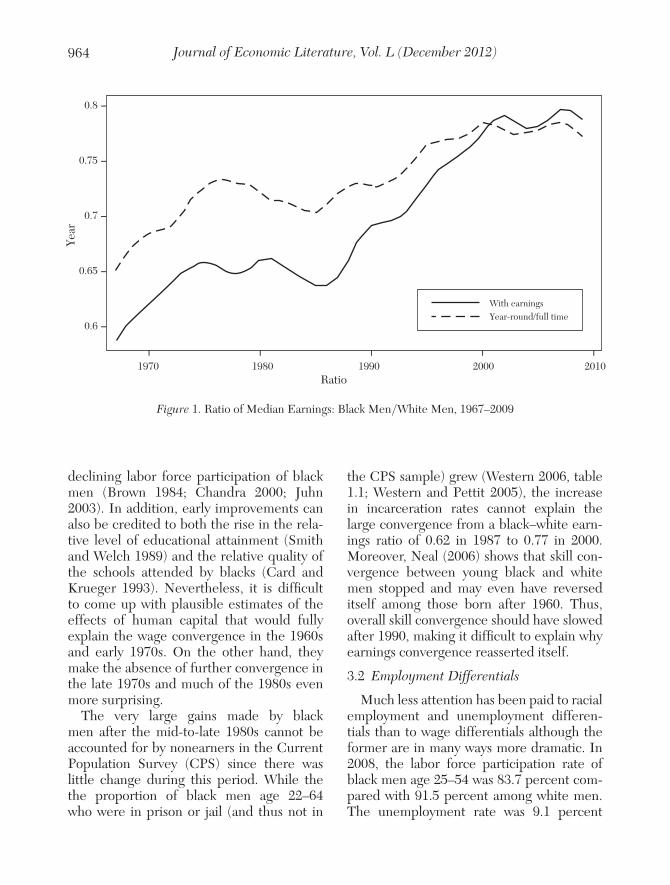
declining labor force participation of black men (Brown 1984; Chandra 2000; Juhn 2003). In addition, early improvements can also be credited to both the rise in the rela‑tive level of educational attainment (Smith and Welch 1989) and the relative quality of the schools attended by blacks (Card and Krueger 1993). Nevertheless, it is difficult to come up with plausible estimates of the effects of human capital that would fully explain the wage convergence in the 1960s and early 1970s. On the other hand, they make the absence of further convergence in the late 1970s and much of the 1980s even more surprising.

The very large gains made by black men after the mid‑to‑late 1980s cannot be accounted for by nonearners in the Current Population Survey (CPS) since there was little change during this period. While the the proportion of black men age 22–64 who were in prison or jail (and thus not in

the CPS sample) grew (Western 2006, table 1.1; Western and Pettit 2005), the increase in incarceration rates cannot explain the large convergence from a black–white earn‑ings ratio of 0.62 in 1987 to 0.77 in 2000. Moreover, Neal (2006) shows that skill con‑vergence between young black and white men stopped and may even have reversed itself among those born after 1960. Thus, overall skill convergence should have slowed after 1990, making it difficult to explain why earnings convergence reasserted itself.

3.2 Employment Differentials

Much less attention has been paid to racial employment and unemployment differen‑tials than to wage differentials although the former are in many ways more dramatic. In 2008, the labor force participation rate of black men age 25–54 was 83.7 percent com‑pared with 91.5 percent among white men. The unemployment rate was 9.1 percent

Year

0.8

0.75

0.7

0.65

0.6

1970 1980 1990 2000 2010

–

–

–

–

–

Ratio

With earningsYear-round/full time

–

– – – –

Figure 1. Ratio of Median Earnings: Black Men/White Men, 1967–2009

Journal of Economic Literature, Vol. L (December 2012)968

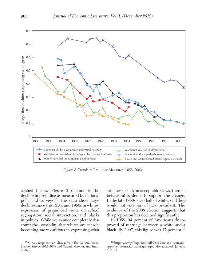
against blacks. Figure 3 documents the decline in prejudice as measured by national polls and surveys.15 The data show large declines since the 1950s and 1960s in whites’ expression of prejudiced views on school segregation, social interaction, and blacks in politics. While we cannot completely dis‑count the possibility that whites are merely becoming more cautious in expressing what

15 Survey responses are drawn from the General Social Society Survey 1972–2008 and Naemi, Mueller, and Smith (1989).

are now socially unacceptable views, there is behavioral evidence to support the change. In the late 1950s, over half of whites said they would not vote for a black president. The evidence of the 2008 election suggests that this proportion has declined significantly.

In 1958, 94 percent of Americans disap‑proved of marriage between a white and a black. By 2007, this figure was 17 percent.16

16 http://www.gallup.com/poll/28417/most‑americans‑approve‑interracial‑marriages.aspx, downloaded January 5, 2010.

Prop

ortio

n of

whi

tes

resp

ondi

ng y

es o

r ag

ree

0.8

0.7

0.6

0.5

0.4

0.3

0.2

0.1

0

–

–

–

–

–

–

–

–

–1956 1960 1964 1968 1972 1976 1980 1984 1988 1992 1996 2000

- - - - - - - - - - - - - - - - - - - - - - - - - - - - - - - - - - - - - - - - - - - - - - - -

There should be a law against interracial marriage

Would object to a friend bringing a black person to dinner

Whites have right to segregate neighborhood

Would not vote for black president

Blacks should not push where not wanted

Blacks and whites should attend separate schools

Figure 3. Trends in Prejudice Measures, 1956–2003.

Table 1Mean Call-Back Rates By Racial Soundingness of Names a

Call-Back Rate for Call-Back Rate for Ratio DifferenceWhite Names African American Names (p-value)

Sample:

All sent resumes 10.06% 6.70% 1.50 3.35%[2445] [2445] (.0000)

Chicago 8.61% 5.81% 1.48 2.80%[1359] [1359] (.0024)

Boston 11.88% 7.83% 1.52 4.05%[1086] [1086] (.0008)

Females 10.33% 6.87% 1.50 3.46%[1868] [1893] (.0001)

Females in administrative jobs 10.93% 6.81% 1.60 4.12%[1363] [1364] (.0001)

Females in sales jobs 8.71% 6.99% 1.25 1.72%[505] [529] (.1520)

Males 9.19% 6.16% 1.49 3.03%[577] [552] (.0283)

aNotes:

1. The table reports, for the entire sample and different subsamples of sent resumes, the call-back rates for applicants witha White sounding name (column 1) and an African American sounding name (column 2), as well as the ratio (column3) and difference (column 4) of these call-back rates. In brackets in each cell is the number of resumes sent in that cell.

2. Column 4 also reports the p-value for a test of proportion testing the null hypothesis that the call-back rates are equalacross racial groups.

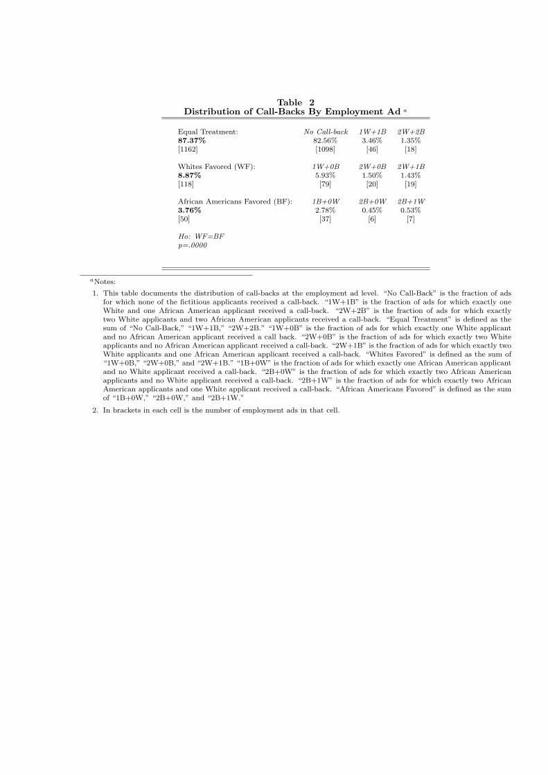
Table 2Distribution of Call-Backs By Employment Ad a

Equal Treatment: No Call-back 1W+1B 2W+2B87.37% 82.56% 3.46% 1.35%[1162] [1098] [46] [18]

Whites Favored (WF): 1W+0B 2W+0B 2W+1B8.87% 5.93% 1.50% 1.43%[118] [79] [20] [19]

African Americans Favored (BF): 1B+0W 2B+0W 2B+1W3.76% 2.78% 0.45% 0.53%[50] [37] [6] [7]

Ho: WF=BFp=.0000

aNotes:

1. This table documents the distribution of call-backs at the employment ad level. “No Call-Back” is the fraction of adsfor which none of the fictitious applicants received a call-back. “1W+1B” is the fraction of ads for which exactly oneWhite and one African American applicant received a call-back. “2W+2B” is the fraction of ads for which exactlytwo White applicants and two African American applicants received a call-back. “Equal Treatment” is defined as thesum of “No Call-Back,” “1W+1B,” “2W+2B.” “1W+0B” is the fraction of ads for which exactly one White applicantand no African American applicant received a call back. “2W+0B” is the fraction of ads for which exactly two Whiteapplicants and no African American applicant received a call-back. “2W+1B” is the fraction of ads for which exactly twoWhite applicants and one African American applicant received a call-back. “Whites Favored” is defined as the sum of“1W+0B,” “2W+0B,” and “2W+1B.” “1B+0W” is the fraction of ads for which exactly one African American applicantand no White applicant received a call-back. “2B+0W” is the fraction of ads for which exactly two African Americanapplicants and no White applicant received a call-back. “2B+1W” is the fraction of ads for which exactly two AfricanAmerican applicants and one White applicant received a call-back. “African Americans Favored” is defined as the sumof “1B+0W,” “2B+0W,” and “2B+1W.”

2. In brackets in each cell is the number of employment ads in that cell.

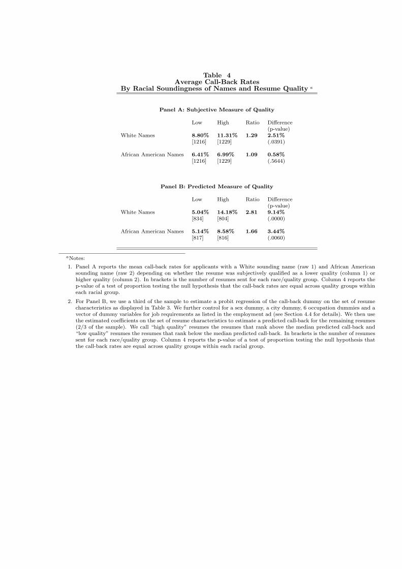
Table 4Average Call-Back Rates

By Racial Soundingness of Names and Resume Quality a

Panel A: Subjective Measure of Quality

Low High Ratio Difference(p-value)

White Names 8.80% 11.31% 1.29 2.51%[1216] [1229] (.0391)

African American Names 6.41% 6.99% 1.09 0.58%[1216] [1229] (.5644)

Panel B: Predicted Measure of Quality

Low High Ratio Difference(p-value)

White Names 5.04% 14.18% 2.81 9.14%[834] [804] (.0000)

African American Names 5.14% 8.58% 1.66 3.44%[817] [816] (.0060)

aNotes:

1. Panel A reports the mean call-back rates for applicants with a White sounding name (raw 1) and African Americansounding name (raw 2) depending on whether the resume was subjectively qualified as a lower quality (column 1) orhigher quality (column 2). In brackets is the number of resumes sent for each race/quality group. Column 4 reports thep-value of a test of proportion testing the null hypothesis that the call-back rates are equal across quality groups withineach racial group.

2. For Panel B, we use a third of the sample to estimate a probit regression of the call-back dummy on the set of resumecharacteristics as displayed in Table 3. We further control for a sex dummy, a city dummy, 6 occupation dummies and avector of dummy variables for job requirements as listed in the employment ad (see Section 4.4 for details). We then usethe estimated coefficients on the set of resume characteristics to estimate a predicted call-back for the remaining resumes(2/3 of the sample). We call “high quality” resumes the resumes that rank above the median predicted call-back and“low quality” resumes the resumes that rank below the median predicted call-back. In brackets is the number of resumessent for each race/quality group. Column 4 reports the p-value of a test of proportion testing the null hypothesis thatthe call-back rates are equal across quality groups within each racial group.

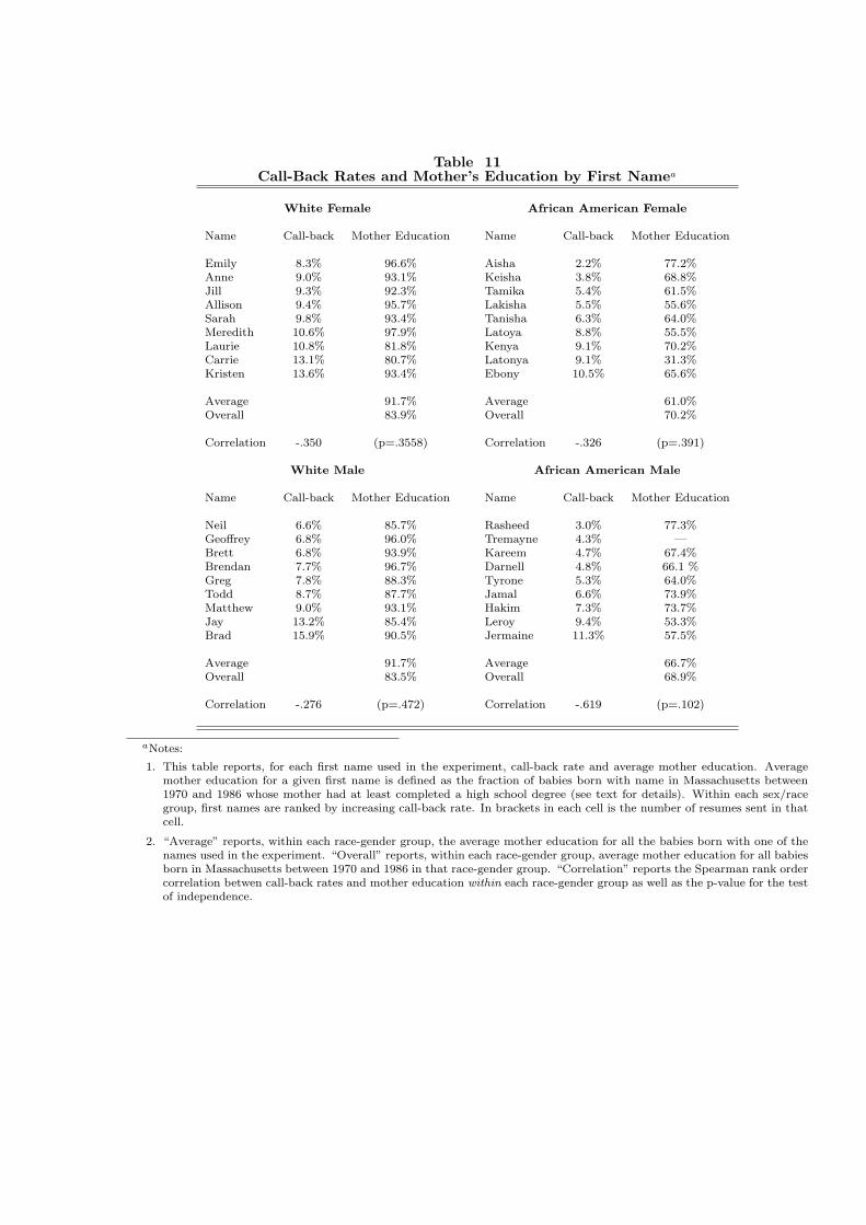
Table 11Call-Back Rates and Mother’s Education by First Namea

White Female African American Female

Name Call-back Mother Education Name Call-back Mother Education

Emily 8.3% 96.6% Aisha 2.2% 77.2%Anne 9.0% 93.1% Keisha 3.8% 68.8%Jill 9.3% 92.3% Tamika 5.4% 61.5%Allison 9.4% 95.7% Lakisha 5.5% 55.6%Sarah 9.8% 93.4% Tanisha 6.3% 64.0%Meredith 10.6% 97.9% Latoya 8.8% 55.5%Laurie 10.8% 81.8% Kenya 9.1% 70.2%Carrie 13.1% 80.7% Latonya 9.1% 31.3%Kristen 13.6% 93.4% Ebony 10.5% 65.6%

Average 91.7% Average 61.0%Overall 83.9% Overall 70.2%

Correlation -.350 (p=.3558) Correlation -.326 (p=.391)

White Male African American Male

Name Call-back Mother Education Name Call-back Mother Education

Neil 6.6% 85.7% Rasheed 3.0% 77.3%Geoffrey 6.8% 96.0% Tremayne 4.3% —Brett 6.8% 93.9% Kareem 4.7% 67.4%Brendan 7.7% 96.7% Darnell 4.8% 66.1 %Greg 7.8% 88.3% Tyrone 5.3% 64.0%Todd 8.7% 87.7% Jamal 6.6% 73.9%Matthew 9.0% 93.1% Hakim 7.3% 73.7%Jay 13.2% 85.4% Leroy 9.4% 53.3%Brad 15.9% 90.5% Jermaine 11.3% 57.5%

Average 91.7% Average 66.7%Overall 83.5% Overall 68.9%

Correlation -.276 (p=.472) Correlation -.619 (p=.102)

aNotes:

1. This table reports, for each first name used in the experiment, call-back rate and average mother education. Averagemother education for a given first name is defined as the fraction of babies born with name in Massachusetts between1970 and 1986 whose mother had at least completed a high school degree (see text for details). Within each sex/racegroup, first names are ranked by increasing call-back rate. In brackets in each cell is the number of resumes sent in thatcell.

2. “Average” reports, within each race-gender group, the average mother education for all the babies born with one of thenames used in the experiment. “Overall” reports, within each race-gender group, average mother education for all babiesborn in Massachusetts between 1970 and 1986 in that race-gender group. “Correlation” reports the Spearman rank ordercorrelation betwen call-back rates and mother education within each race-gender group as well as the p-value for the testof independence.

JURY RACE AND CRIMINAL TRIALS 13

TABLE I

SUMMARY STATISTICS

All Cases Black Defendants White Defendants

Mean Std. dev. Mean Std. dev. Mean Std. dev.

Defendantcharacteristics

Black 0.44 0.50 1 0 0 0Hispanic 0.04 0.20 0 0 0 0White 0.51 0.50 0 0 1 0Male 0.92 0.27 0.95 0.21 0.89 0.32

Case characteristicsTotal charges 2.99 3.57 2.79 2.33 3.26 4.55Any drug charge 0.25 0.44 0.37 0.49 0.14 0.35Any murder charge 0.05 0.22 0.06 0.25 0.05 0.21Any robbery charge 0.09 0.29 0.15 0.36 0.05 0.21Any other violent

charge 0.31 0.46 0.31 0.46 0.30 0.46Any property charge 0.23 0.42 0.21 0.41 0.25 0.43Any sex charge 0.13 0.34 0.08 0.27 0.18 0.38Any weapons charge 0.12 0.33 0.18 0.39 0.08 0.27Any other charge 0.33 0.47 0.26 0.44 0.37 0.48

Dependant variablesProportion guilty

convictions 0.670 0.439 0.686 0.432 0.641 0.450Any guilty convictions 0.728 0.445 0.745 0.437 0.702 0.458

Pool and seated jurycharacteristics

Number of seatedjurors 7.11 0.483 7.12 0.476 7.11 0.496

Number in jury pool 27.3 7.3 26.9 7.0 27.6 7.6Any black in pool 0.64 0.48 0.63 0.48 0.65 0.48Any black on seated

jury 0.28 0.45 0.29 0.45 0.26 0.44Proportion black on

seated jury 0.046 0.080 0.051 0.089 0.040 0.069Proportion black in

pool 0.039 0.040 0.040 0.043 0.038 0.038

Observations 785 333 379

Notes: The first two columns report summary statistics for the full sample of 785 cases for which a jurywas selected and the variable under consideration is defined. In particular, defendant race is defined for 774cases, defendant gender for 776 cases, specific crime categories for 776 cases, total charges for 773 cases, thedependant variables for 750 cases, and the pool and seated jury variables for the full sample of 785 cases.The latter columns report summary statistics for cases with black defendants (n = 333) and white defendants(n = 379), respectively, in which a verdict of guilty or not guilty by the jury was returned for at least oneof the charged offenses. Together, the observations in these columns make up the sample used in our mainanalysis. Summary statistics for the proportion variables (i.e., proportion guilty convictions, proportion blackon seated jury, and proportion black in pool) were formed by measuring the proportion for each jury or jurypool and averaging across cases.

at University of C

alifornia School of Law

(Boalt H

all) on Decem

ber 2, 2014http://qje.oxfordjournals.org/

Dow

nloaded from

JURY RACE AND CRIMINAL TRIALS 15

TABLE II

THE RELATIONSHIP BETWEEN THE RACIAL COMPOSITION OF THE JURY POOL ANDDEFENDANT/CASE CHARACTERISTICS

(1) (2) (3) (4)Indicator forany blacks

in pool

Proportionof blacks in

pool

Proportionof whites in

pool

Proportionof other

races in pool

Defendant characteristics

Black −0.008 0.003 −0.004 0.001[0.039] [0.003] [0.005] [0.003]

Hispanic 0.005 0.004 −0.003 −0.001[0.088] [0.008] [0.011] [0.006]

Male 0.043 0.006 −0.009 0.002[0.067] [0.005] [0.007] [0.004]

Case characteristicsAny drug charge −0.029 −0.0003 0.004 −0.003

[0.051] [0.004] [0.006] [0.004]Any murder charge 0.093 −0.002 −0.006 0.006

[0.076] [0.006] [0.008] [0.005]Any other charge 0.007 0.002 −0.004 −0.0005

[0.040] [0.004] [0.005] [0.003]Any other violent charge 0.0001 0.004 −0.004 −0.0003

[0.042] [0.004] [0.005] [0.003]Any property charge 0.078 0.013∗∗∗ −0.006 −0.008∗∗

[0.047] [0.005] [0.006] [0.003]Any robbery charge −0.026 −0.005 0.004 0.0001

[0.065] [0.005] [0.008] [0.005]Any sex charge 0.07 0.002 0.001 −0.004

[0.058] [0.005] [0.006] [0.004]Any weapons charge 0.075 −0.001 0.001 0.0002

[0.054] [0.004] [0.006] [0.004]Total charges 0.008∗ 5 × 10−5 0.0002 −0.0003

[0.003] [0.000] [0.000] [0.000]Constant 0.541∗∗∗ 0.028∗∗∗ 0.942∗∗∗ 0.029∗∗∗

[0.074] [0.006] [0.007] [0.005]

Observations 771 771 771 771F-statistic 1.40 1.13 0.68 1.07R-squared 0.02 0.02 0.01 0.01

Notes: Each column reports parameter estimates and heteroskedasticity-robust standard errors fromOLS regressions using the variable in the column heading as the dependent variable. *, **, and *** indicatestatistical significance at the 10%, 5%, and 1% levels, respectively. The crime categories are not mutuallyexclusive, so there is no omitted crime category. F-statistics jointly testing whether all coefficients equal0 are reported in the second to last row of the table. Fourteen observations from the full sample shown inTable I were dropped due to one or more missing values for the various defendant and case characteristics.

at University of C

alifornia School of Law

(Boalt H

all) on Decem

ber 2, 2014http://qje.oxfordjournals.org/

Dow

nloaded from

18 QUARTERLY JOURNAL OF ECONOMICS

TABLE IV

REDUCED-FORM BENCHMARK REGRESSIONS

(1) (2) (3) (4)

Dependent variable Any guilty convictionProportion guilty

convictions

Black defendant 0.150∗∗∗ 0.164∗∗∗ 0.156∗∗∗ 0.160∗∗∗

[0.056] [0.058] [0.055] [0.057]Any black in pool 0.069 0.105∗∗ 0.063 0.090∗

[0.048] [0.051] [0.047] [0.050]Black defendant * any

black in pool−0.168∗∗ −0.166∗∗ −0.174∗∗ −0.155∗∗

[0.070] [0.074] [0.069] [0.072]Constant 0.656∗∗∗ 0.627∗∗∗ 0.600∗∗∗ 0.576∗∗∗

[0.039] [0.041] [0.038] [0.040]Includes controls for:Gender/age of pool No Yes No YesCounty dummy No Yes No YesYear of filing dummies No Yes No YesObservations 712 712 712 712R-squared 0.01 0.07 0.01 0.08

Notes: The dependent variable for each regression is shown in the row heading. All regressions areestimated on the main analysis sample using OLS and heteroskedasticity-robust standard errors arereported in brackets. The gender of the jury pool is measured as the proportion of the pool that is female, andthe age of jury pool is controlled for with the proportion of the pool that is age 40 or less, and proportion ofthe pool that is between the ages of 40 and 60. For each of the controls (including county and year of filingdummies) both a demeaned version of the control variable and the interaction of this demeaned variable withwhether the defendant is black are included in the specification. Because the control variables are demeaned,the coefficients on the variables reported in the table can be interpreted as the estimated effect at the meanand are comparable across columns. *, **, and *** indicate statistical significance at the 10%, 5%, and 1%levels, respectively.

ageandaddingyeardummies addresses thepossibilitythat crimepatterns or convictions rates may be trending systematically overtime. In all cases, the additional control variables describedaboveare fully interacted with the defendant’s race. This allows for thepossibility that these control variables have a differential effectfor black and white defendants, just as we have allowed for theracial composition of the jury pool.24

The point estimates for the three key coefficients are re-markably robust and statistically significant in the specificationthat includes controls. For expositional convenience, we use thespecification reported in column (2) as our benchmark specifi-

24. In addition, each control variable is demeaned (prior to being interacted),which ensures that the main coefficients in Table IV are reported at the samplemean in each specification and therefore comparable; that is, there is no needto look at the coefficients on the interaction variables included in the vector ofcontrols.

at University of C

alifornia School of Law

(Boalt H

all) on Decem

ber 2, 2014http://qje.oxfordjournals.org/

Dow

nloaded from

Tab

le2

A

Rac

ial

Dif

fere

nce

sin

No

n-L

eth

alU

seo

fF

orc

e,N

YC

Sto

pQ

ues

tio

nan

dF

risk

,Any

Use

of

Fo

rce

Wh

ite

Mea

nB

lack

His

pan

icA

sian

Oth

erR

ace

(1)

(2)

(3)

(4)

(5)

No

Co

ntr

ols

0.1

53

1.5

34∗∗∗

1.5

82∗∗∗

1.0

44

1.3

92∗∗∗

(0.1

44

)(0

.14

9)

(0.1

19

)(0

.12

1)

+B

asel

ine

Ch

arac

teri

stic

s1.4

80∗∗∗

1.5

17∗∗∗

1.0

10

1.3

46∗∗∗

(0.1

46

)(0

.14

6)

(0.1

22

)(0

.11

4)

+E

nco

un

ter

Ch

arac

teri

stic

s1.6

55∗∗∗

1.6

41∗∗∗

1.0

59

1.4

52∗∗∗

(0.1

55

)(0

.15

7)

(0.1

33

)(0

.12

1)

+C

ivil

ian

Beh

avio

r1.4

56∗∗∗

1.5

13∗∗∗

1.0

49

1.3

68∗∗∗

(0.1

28

)(0

.13

6)

(0.1

24

)(0

.10

7)

+F

ixed

Eff

ects

1.1

73∗∗∗

1.1

20∗∗∗

0.9

51

1.0

57∗∗

(0.0

34

)(0

.02

6)

(0.0

33

)(0

.02

8)

Ob

serva

tio

ns

4,9

27

,46

7

No

tes:

Th

ista

ble

rep

ort

so

dd

sra

tio

sb

yru

nn

ing

log

isti

cre

gre

ssio

ns.

Th

esa

mp

leco

nsi

sts

of

all

NY

Cst

op

and

fris

ks

fro

m2

00

3-2

01

3

wit

hn

on

-mis

sin

gu

seo

ffo

rce

dat

a.T

he

dep

end

ent

var

iab

leis

anin

dic

ato

rfo

rw

het

her

the

po

lice

rep

ort

edu

sin

gan

yfo

rce

du

rin

ga

sto

p

and

fris

kin

tera

ctio

n.

Th

eo

mit

ted

race

isw

hit

e,an

dth

eo

mit

ted

IDty

pe

iso

ther

.T

he

firs

tco

lum

ng

ives

the

un

con

dit

ion

alav

erag

eo

fst

op

and

fris

kin

tera

ctio

ns

that

rep

ort

edan

yfo

rce

bei

ng

use

dfo

rw

hit

eci

vil

ian

s.C

olu

mn

s(2

)th

rou

gh

(5)

rep

ort

log

isti

ces

tim

ates

for

bla

ck,

his

pan

ic,

asia

nan

do

ther

race

civ

ilia

ns

resp

ecti

vel

y.E

ach

row

corr

esp

on

ds

toa

dif

fere

nt

emp

iric

alsp

ecifi

cati

on

.T

he

firs

tro

win

clu

des

sole

lyra

cial

gro

up

du

mm

ies.

Th

ese

con

dro

wad

ds

con

tro

lsfo

rg

end

eran

da

qu

adra

tic

inag

e.T

he

thir

dro

wad

ds

con

tro

lsfo

rw

het

her

the

sto

pw

asin

do

ors

or

ou

tdo

ors

,w

het

her

the

sto

pto

ok

pla

ced

uri

ng

the

day

tim

e,w

het

her

the

sto

pto

ok

pla

cein

ah

igh

crim

ear

eao

r

du

rin

ga

hig

hcr

ime

tim

e,w

het

her

the

offi

cer

was

inu

nif

orm

,ci

vil

ian

IDty

pe,

and

wh

eth

ero

ther

sw

ere

sto

pp

edd

uri

ng

the

inte

ract

ion

.

Th

efo

urt

hro

wad

ds

con

tro

lsfo

rci

vil

ian

beh

avio

r.T

he

fift

hro

wad

ds

pre

cin

ctan

dy

ear

fixed

effe

cts.

Eac

hro

win

clu

des

mis

sin

gs

inal

l

var

iab

les.

Sta

nd

ard

erro

rscl

ust

ered

atth

ep

reci

nct

level

are

rep

ort

edin

par

enth

eses

.

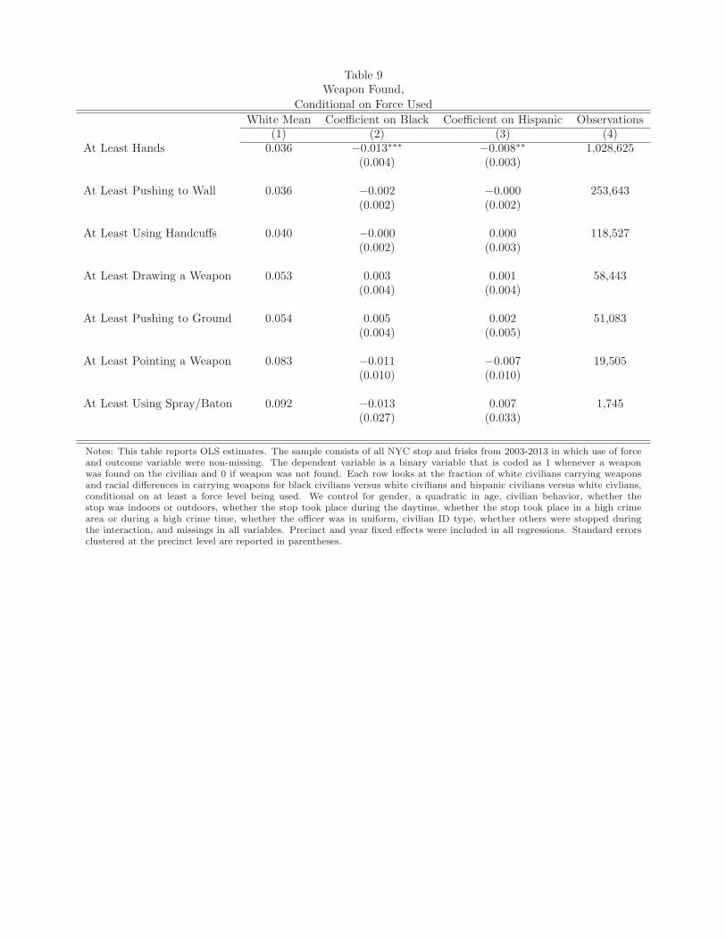
Table 9Weapon Found,

Conditional on Force Used

White Mean Coefficient on Black Coefficient on Hispanic Observations(1) (2) (3) (4)

At Least Hands 0.036 −0.013∗∗∗ −0.008∗∗ 1,028,625(0.004) (0.003)

At Least Pushing to Wall 0.036 −0.002 −0.000 253,643(0.002) (0.002)

At Least Using Handcuffs 0.040 −0.000 0.000 118,527(0.002) (0.003)

At Least Drawing a Weapon 0.053 0.003 0.001 58,443(0.004) (0.004)

At Least Pushing to Ground 0.054 0.005 0.002 51,083(0.004) (0.005)

At Least Pointing a Weapon 0.083 −0.011 −0.007 19,505(0.010) (0.010)

At Least Using Spray/Baton 0.092 −0.013 0.007 1,745(0.027) (0.033)

Notes: This table reports OLS estimates. The sample consists of all NYC stop and frisks from 2003-2013 in which use of force

and outcome variable were non-missing. The dependent variable is a binary variable that is coded as 1 whenever a weapon

was found on the civilian and 0 if weapon was not found. Each row looks at the fraction of white civilians carrying weapons

and racial differences in carrying weapons for black civilians versus white civilians and hispanic civilians versus white civlians,

conditional on at least a force level being used. We control for gender, a quadratic in age, civilian behavior, whether the

stop was indoors or outdoors, whether the stop took place during the daytime, whether the stop took place in a high crime

area or during a high crime time, whether the officer was in uniform, civilian ID type, whether others were stopped during

the interaction, and missings in all variables. Precinct and year fixed effects were included in all regressions. Standard errors

clustered at the precinct level are reported in parentheses.

44

Figure 3: Booking Rates by Age and Race, All Juvenile Arrests and First Arrests

Figure 4: Arrest Status by Arrest Sequence and Race/Ethnicity for those Youth Arrested at Least Four Times

.2.3

.4.5

.6Pr

oport

ion Bo

oked

10 12 14 16 18age

Black HispanicWhite

All Juvenile Arrests

.2.3

.4.5

.6Pr

oport

ion Bo

oked

10 12 14 16 18age

Black HispanicWhite

First Arrests

0.460.53

0.580.64

0.380.42

0.460.51

0.350.39

0.440.49

0.2

.4.6

Pro

porti

on B

ooke

d

Black Hispanic White1 2 3 4 1 2 3 4 1 2 3 4

0.410.36

0.320.27

0.450.42

0.390.35

0.470.44

0.390.36

0.1

.2.3

.4.5

Pro

porti

on C

ited

Black Hispanic White1 2 3 4 1 2 3 4 1 2 3 4

0.130.11

0.100.09

0.170.15

0.140.13

0.18 0.17 0.160.15

0.0

5.1

.15

.2P

ropo

rtion

Oth

er

Black Hispanic White1 2 3 4 1 2 3 4 1 2 3 4

45

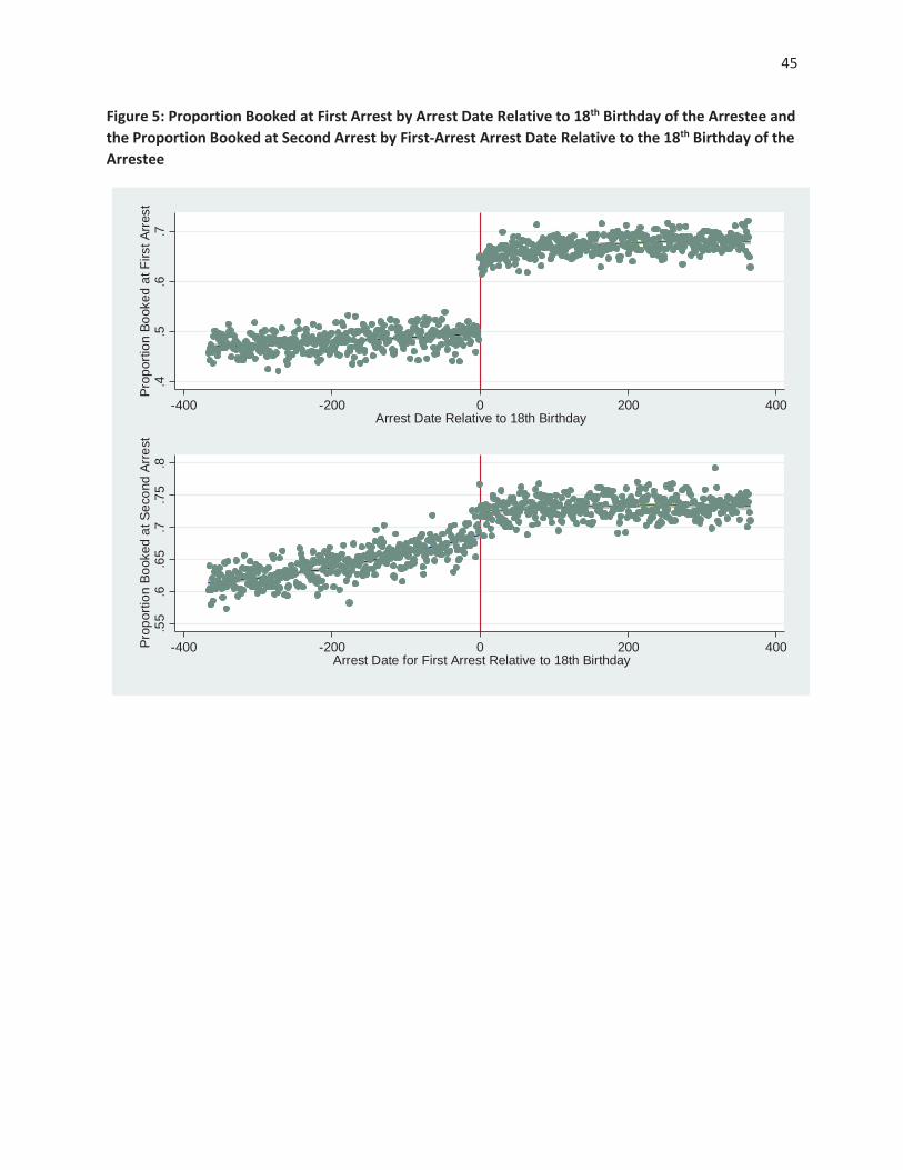
Figure 5: Proportion Booked at First Arrest by Arrest Date Relative to 18th Birthday of the Arrestee and the Proportion Booked at Second Arrest by First-Arrest Arrest Date Relative to the 18th Birthday of the Arrestee

.4.5

.6.7

Prop

ortio

n Bo

oked

at F

irst A

rres

t

-400 -200 0 200 400Arrest Date Relative to 18th Birthday

.55

.6.6

5.7

.75

.8Pr

opor

tion

Book

ed a

t Sec

ond

Arre

st

-400 -200 0 200 400Arrest Date for First Arrest Relative to 18th Birthday

47

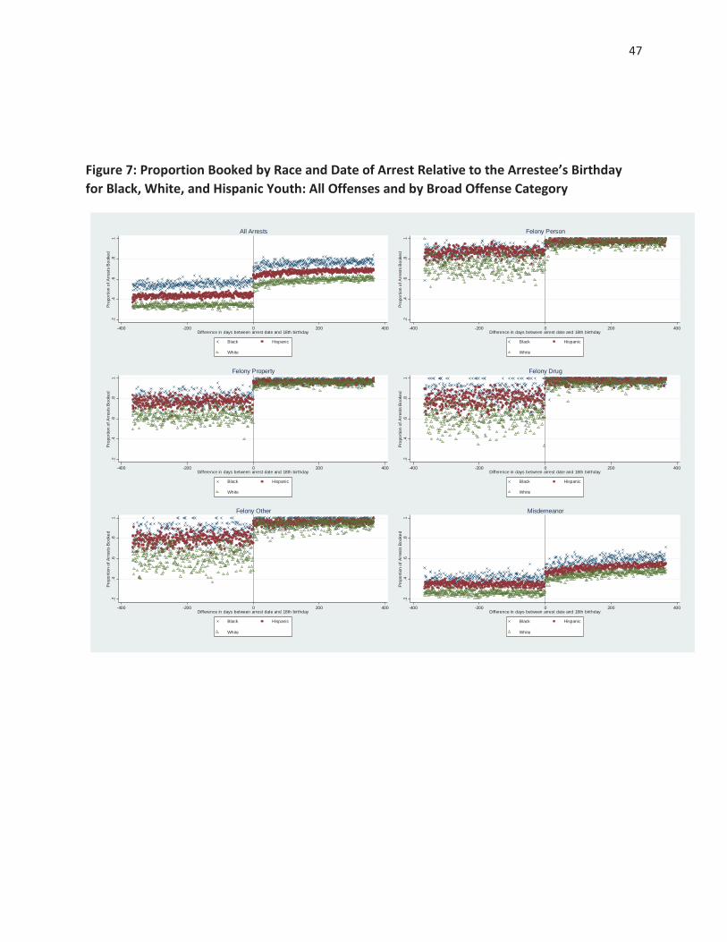
Figure 7: Proportion Booked by Race and Date of Arrest Relative to the Arrestee’s Birthday for Black, White, and Hispanic Youth: All Offenses and by Broad Offense Category

.2.4

.6.8

1P

ropo

rtion

of A

rres

ts B

ooke

d

-400 -200 0 200 400Difference in days between arrest date and 18th birthday

Black Hispanic

White

All Arrests

.2.4

.6.8

1P

ropo

rtion

of A

rres

ts B

ooke

d

-400 -200 0 200 400Difference in days between arrest date and 18th birthday

Black Hispanic

White

Felony Person

.2.4

.6.8

1P

ropo

rtion

of A

rres

ts B

ooke

d

-400 -200 0 200 400Difference in days between arrest date and 18th birthday

Black Hispanic

White

Felony Property

.2.4

.6.8

1P

ropo

rtion

of A

rres

ts B

ooke

d

-400 -200 0 200 400Difference in days between arrest date and 18th birthday

Black Hispanic

White

Felony Drug

.2.4

.6.8

1P

ropo

rtion

of A

rres

ts B

ooke

d

-400 -200 0 200 400Difference in days between arrest date and 18th birthday

Black Hispanic

White

Felony Other

.2.4

.6.8

1P

ropo

rtion

of A

rres

ts B

ooke

d

-400 -200 0 200 400Difference in days between arrest date and 18th birthday

Black Hispanic

White

Misdemeanor

52

Table 4 IV Estimates of the Effect of a Prior Booking on the Likelihood that the Current Arrest is Booked Exploiting the Discontinuous Increases in Bookings Occurring at the Age of 18 Sample Specification (1) Specification (2) Specification (3) All Arrests 0.239 (0.024)a 0.117 (0.027)a 0.112 (0.026)a

Felony arrests 0.045 (0.017)a 0.055 (0.027)b 0.043 (0.025)c

Misdemeanor arrests 0.388 (0.034)a 0.164 (0.039)a 0.150 (0.036)a

Black 0.202 (0.065)a 0.110 (0.072) 0.109 (0.066)c

White 0.246 (0.037)a 0.161 (0.038)a 0.139 (0.036)a

Hispanic 0.224 (0.039)a 0.048 (0.051) 0.072 (0.045) Male 0.204 (0.025)a 0.083 (0.028)a 0.075 (0.027)a

Female 0.460 (0.069)a 0.342 (0.092)a 0.331 (0.082)a

Standard errors are in parentheses. Estimates are based on a just-identified 2SLS model where the first stage includes the arrest date for the first arrest relative to the arrestees 18th birthday, the date variable squared, a dummy for over 18, interaction terms between the dummy and the quadratic function for the running variable and various additional covariates. Specification (1) only includes these variables. Specification (2) adds dummy variables for race and ethnicity, gender, the first arrest offense (roughly 76 categories), and the current arrest offense (roughly 72 categories). The final specification adds over 700 fixed effects for arresting agency.

a. Statistically significant at the one percent level of confidence. b. Statistically significant at the five percent level of confidence. c. Statistically significant at the ten percent level of confidence.

53

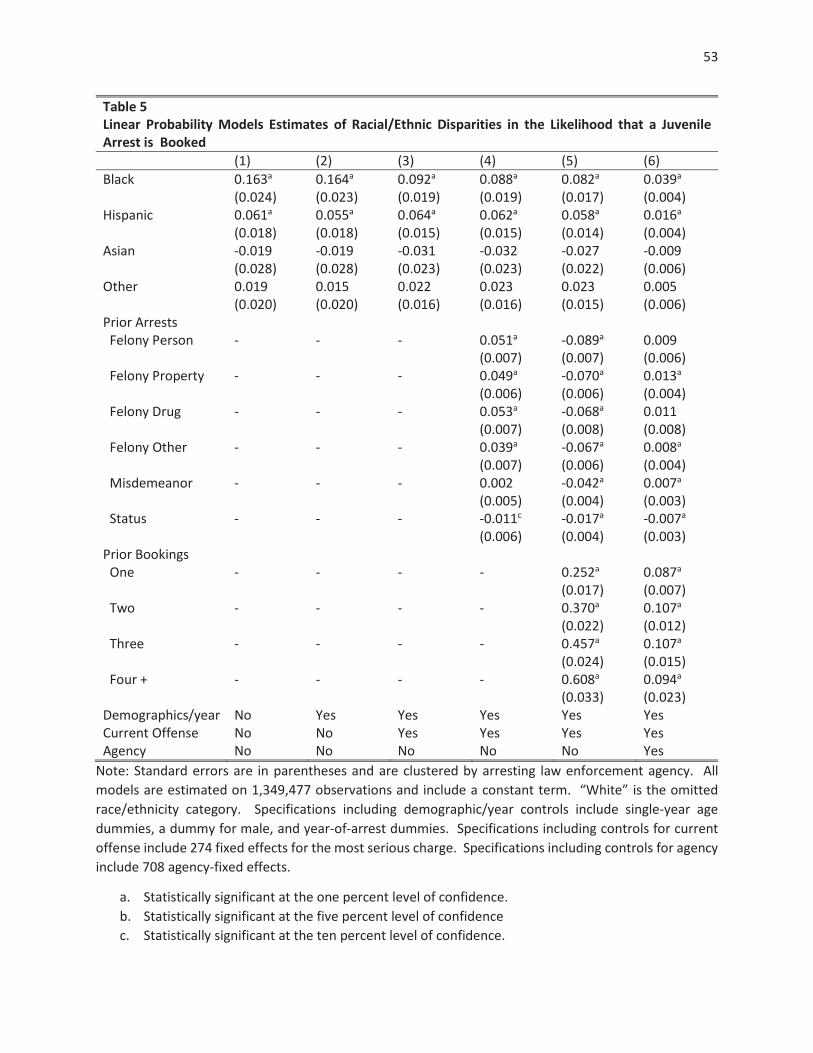
Table 5 Linear Probability Models Estimates of Racial/Ethnic Disparities in the Likelihood that a Juvenile Arrest is Booked (1) (2) (3) (4) (5) (6) Black 0.163a

(0.024) 0.164a

(0.023) 0.092a

(0.019) 0.088a

(0.019) 0.082a

(0.017) 0.039a

(0.004) Hispanic 0.061a

(0.018) 0.055a

(0.018) 0.064a

(0.015) 0.062a

(0.015) 0.058a

(0.014) 0.016a

(0.004) Asian -0.019

(0.028) -0.019 (0.028)

-0.031 (0.023)

-0.032 (0.023)

-0.027 (0.022)

-0.009 (0.006)

Other 0.019 (0.020)

0.015 (0.020)

0.022 (0.016)

0.023 (0.016)

0.023 (0.015)

0.005 (0.006)

Prior Arrests Felony Person - - - 0.051a

(0.007) -0.089a

(0.007) 0.009 (0.006)

Felony Property - - - 0.049a

(0.006) -0.070a

(0.006) 0.013a

(0.004) Felony Drug - - - 0.053a

(0.007) -0.068a

(0.008) 0.011 (0.008)

Felony Other - - - 0.039a

(0.007) -0.067a

(0.006) 0.008a

(0.004) Misdemeanor - - - 0.002

(0.005) -0.042a

(0.004) 0.007a

(0.003) Status - - - -0.011c

(0.006) -0.017a

(0.004) -0.007a

(0.003) Prior Bookings One - - - - 0.252a

(0.017) 0.087a

(0.007) Two - - - - 0.370a

(0.022) 0.107a

(0.012) Three - - - - 0.457a

(0.024) 0.107a

(0.015) Four + - - - - 0.608a

(0.033) 0.094a

(0.023) Demographics/year No Yes Yes Yes Yes Yes Current Offense No No Yes Yes Yes Yes Agency No No No No No Yes

Note: Standard errors are in parentheses and are clustered by arresting law enforcement agency. All models are estimated on 1,349,477 observations and include a constant term. “White” is the omitted race/ethnicity category. Specifications including demographic/year controls include single-year age dummies, a dummy for male, and year-of-arrest dummies. Specifications including controls for current offense include 274 fixed effects for the most serious charge. Specifications including controls for agency include 708 agency-fixed effects.

a. Statistically significant at the one percent level of confidence. b. Statistically significant at the five percent level of confidence c. Statistically significant at the ten percent level of confidence.