racoro science and operations plan · racoro science and operations plan december 2008 dr. andrew...
TRANSCRIPT
DOE/SC-ARM-0806
RACORO Science and Operations Plan December 2008 Dr. Andrew M. Vogelmann, Principal Investigator* RACORO Steering Committee (RSC): Andrew Vogelmann – Brookhaven National Laboratory Greg McFarquhar – University of Illinois John Ogren and Graham Feingold – NOAA/Earth System Research Laboratory Dave Turner – University of Wisconsin-Madison Jennifer Comstock and Chuck Long – Pacific Northwest National Laboratory ARM Aerial Vehicles Program (AVP) Technical Operations Office Beat Schmid and Jason Tomlinson – Pacific Northwest National Laboratory Center for Interdisciplinary Remotely-Piloted Aircraft Studies (CIRPAS) Haf Jonsson – Naval Postgraduate School *Brookhaven National Laboratory Bldg 490-D Upton, NY 11973 Tel: (631)-344-4421, Fax: (631) 344-2060 e-mail: [email protected] Work supported by the U.S. Department of Energy, Office of Science, Office of Biological and Environmental Research

DISCLAIMER This report was prepared as an account of work sponsored by the U.S. Government. Neither the United States nor any agency thereof, nor any of their employees, makes any warranty, express or implied, or assumes any legal liability or responsibility for the accuracy, completeness, or usefulness of any information, apparatus, product, or process disclosed, or represents that its use would not infringe privately owned rights. Reference herein to any specific commercial product, process, or service by trade name, trademark, manufacturer, or otherwise, does not necessarily constitute or imply its endorsement, recommendation, or favoring by the U.S. Government or any agency thereof. The views and opinions of authors expressed herein do not necessarily state or reflect those of the U.S. Government or any agency thereof.

A. Vogelmann, December 2008, DOE/SC-ARM-0806
iii
Executive Summary
Our knowledge of boundary layer clouds and their cloud processes is insufficient to resolve pressing scientific problems. Boundary layer clouds often have liquid-water paths (LWPs) less than 100 g m-2, which are defined here as being “thin” Clouds with Low Optical Water Depths (CLOWD). This type of cloud is common globally, and the Earth’s radiative energy balance is particularly sensitive to small changes in their LWPs. However, it is difficult to retrieve accurately their cloud properties because they are tenuous and often broken, which interferes with our ability to obtain the routine, long-term statistics needed to resolve associated uncertainties in climate models. To resolve this dilemma, a better understanding of this cloud type is needed that can only be achieved by acquiring in situ data that are needed for process studies and for evaluation and refinement of existing retrieval algorithms from ground-based instruments.
Coordinated by the ARM Aerial Vehicles Program (AVP), the Routine AVP CLOWD Optical Radiative Observations (RACORO) field campaign will fill this knowledge gap by conducting long-term, systematic flights in boundary layer, liquid-water clouds over the ARM Climate Research Facility (ACRF) Southern Great Plains site. Operating between 22 January and 30 June 2009, this is the first time that a long-term aircraft campaign has been undertaken for systematic in situ sampling of cloud properties. The Center for Interdisciplinary Remotely-Piloted Aircraft Studies (CIRPAS) Twin Otter aircraft, equipped with a full payload of research instrumentation, will be used to obtain representative statistics of cloud microphysical, aerosol, and radiative properties of the atmosphere. These data will be used to validate retrieval algorithms and support process studies and model simulations of boundary layer clouds and, in particular, CLOWD-type clouds.
This Science and Operations Plan articulates the types of science questions to be addressed and the associated instrument payload and flight measurement strategies that will be used to obtain the needed data. For RACORO to operate as a routine, long-term program, flight operations must be kept as simple as possible to achieve its objectives, which require an operating paradigm different from typical, short-term, intensive aircraft field programs. These operating procedures are described for flight plans and scheduling, program management and command structure, data quality control and data dissemination, and project monitoring and reporting.

A. Vogelmann, December 2008, DOE/SC-ARM-0806
iv
Contents
1. Introduction ........................................................................................................................................... 1 2. Overview of RACORO ......................................................................................................................... 3 3. RACORO Science Questions ................................................................................................................ 3 4. Instruments and Measurements ............................................................................................................. 5 5. Sampling Needs .................................................................................................................................... 8 6. Sampling Strategy ............................................................................................................................... 11
6.1 Daytime Cloud Flights ............................................................................................................ 13 6.2 Nighttime Cloud Flights .......................................................................................................... 18 6.3 Daytime Clear-Sky Flights ...................................................................................................... 18 6.4 Flight Safety ............................................................................................................................ 19
7. Flight Scheduling and Execution ........................................................................................................ 20 7.1 Flight Schedule ........................................................................................................................ 20 7.2 Flight Holds ............................................................................................................................. 21 7.3 Go/No-Go Decision Making ................................................................................................... 21 7.4 Flight Day Schedule of Events ................................................................................................ 22 7.5 Coordination with Other Field Programs ................................................................................ 23
8. Field Program Management ................................................................................................................ 23 8.1 Personnel Involved in Routine Operations .............................................................................. 23 8.2 Personnel Responsibilities ....................................................................................................... 24
9. Program Reporting and Information Dissemination ........................................................................... 25 10. Program Monitoring and Reviews ...................................................................................................... 26
10.1 Flight Day ................................................................................................................................ 26 10.2 Weekly RSC Executive Board Telecons ................................................................................. 26 10.3 Mid-Program Review .............................................................................................................. 27 10.4 Final Program Review ............................................................................................................. 27
11. RACORO Data QC and Dissemination .............................................................................................. 27 11.1 Immediate Processing and Reporting ...................................................................................... 27 11.2 RACORO Instrument PI QC and Reporting ........................................................................... 28 11.3 Data Dissemination ................................................................................................................. 28
12. References ........................................................................................................................................... 28 Appendix A: Satellite Overpass Times ....................................................................................................... 30 Appendix B: Monitored SGP CF Instrumentation ...................................................................................... 34

A. Vogelmann, December 2008, DOE/SC-ARM-0806
v
Figures 1. Frequency distribution of liquid-water paths at three ACRF sites ................................................... 1 2. Triangular flight circuits ................................................................................................................ 14 3. General plan flight levels ............................................................................................................... 14
Tables 1. RACORO instrumentation. .............................................................................................................. 7 2. Science objective 1: cloud radiative forcing and validation of remotely sensed
cloud properties. ............................................................................................................................... 8 3. Science objective 2: improve cloud simulations in climate models. ............................................... 9 4. Science objective 3: investigate aerosol-cloud interactions. .......................................................... 10 5. National Weather Service CLOWD types ..................................................................................... 12 6. Cloud structure categorization, based on Table 5 cloud classifications. ........................................ 13 7. Summary of flight patterns and considerations .............................................................................. 16 8. Summary of clear-sky flights. ........................................................................................................ 19 9. Critical instrumentation ................................................................................................................. 22

A. Vogelmann, December 2008, DOE/SC-ARM-0806
1
1. Introduction
The spread of climate sensitivity estimates among general circulation models (GCMs) arises primarily from inter-model differences in the representations of aerosol and cloud processes (IPCC, 2007); in particular, low-level, boundary-layer clouds constitute the largest uncertainty in climate models. This is due to large discrepancies in the radiative responses simulated by models in regions dominated by low-level cloud cover and to the large areas of the globe covered by these regions. Thin, low-level cloud properties are very sensitive to changes in aerosol loading, and the aerosol effect on cloud albedo remains the dominant uncertainty in radiative forcing (IPCC, 2007).
Many boundary layer clouds have liquid-water paths (LWPs) less than 100 g m-2 that are defined here as being “thin” Clouds with Low Optical Water Depths (CLOWD). From the tropics to the Arctic, about 50% or more of the liquid-water clouds have LWPs below this limit (Figure 1). Many types of boundary layer clouds fall into this category, including stratus decks, cumulus fields, and mixed-phase clouds. Because the Earth’s radiative energy balance is particularly sensitive to small perturbations in LWP, small uncertainties in cloud optical properties can affect changes in the local radiative energy balance in excess of that for doubled carbon dioxide (Turner et al., 2007). Thus, particularly accurate retrievals of LWP are required to determine their role in climate and evaluate their simulation in climate models.
The accurate retrieval of microphysical and optical properties of liquid water clouds from remote sensors would seem, at first, to be a solved problem, since these clouds are low in the atmosphere (enabling easier in situ observation) and are composed of spherical droplets whose scattering is well-described by Mie theory. However, a recent intercomparison of 18 state-of-the-art retrieval algorithms showed that – for a simple, warm, single-layer stratiform cloud – the retrieved LWPs differed by 50% to 100% (Turner et al., 2007). Furthermore, ARM’s primary workhorse for observing LWP is a 2-channel microwave radiometer (MWR), which obtains LWP by inverting the measured microwave sky brightness temperatures. However, this study also showed that applying commonly used algorithms to the same observed brightness temperatures can yield LWPs that differ by 50 to 100%.
Figure 1. Frequency distribution of liquid-water paths (LWP) at three ACRF sites. The locations are the North Slope of Alaska at Barrow (NSA), the Southern Great Plains at Lamont, OK (SGP), and the Tropical Western Pacific at Nauru Island (TWP). LWP data are for 2004 as retrieved from a microwave radiometer (MWR) when the cloud base was below 3 km. The frequency distributions indicate a preponderance of clouds with LWPs below 100 g m-2. The LWP distributions for each site are given as [1st quartile, median, 3rd quartile] g m-2:
NSA = [27, 58, 125] g m-2 SGP = [54, 126, 309] g m-2 TWP = [43, 82, 183] g m-2
Figure adapted from Turner et al. (2006).
A. Vogelmann, December 2008, DOE/SC-ARM-0806
2
These differences are unacceptably large, particularly given the importance of these clouds to climate issues that require accurate retrievals for observation, monitoring, and evaluation of model simulations. The prevalence of this type of cloud globally suggests that a dedicated observation program in one location that improves our retrievals would have far reaching benefits to our understanding boundary layer clouds over continents and oceans, the latter having an unusually large importance to climate. Research areas that would benefit are:
• Model parameterizations of continental boundary layer fair-weather cumulus and stratus do not agree well with observations (Lenderink et al., 2004), partly because they are based on simplified mass-flux cumulus parameterizations that use simplified closure assumptions and overly simplified drizzle representations.
• Subtropical marine boundary layer (MBL) clouds largely fall within the CLOWD LWP regime. The albedos of MBL clouds are a particular concern for climate since models simulate them poorly (Zhang et al., 2005; Bender et al., 2006; Zhu et al., 2005). Yet, their simulation and response to changing environmental conditions is the main source of uncertainty in tropical cloud feedbacks simulated by climate models (Bony and Dufresne, 2005).
• The degree of brokenness in MBL cloud fields has a large impact on the global radiative energy budget because of the large albedo difference between the dark ocean and bright stratocumulus sheets. However, retrieving cloud properties within broken fields is even more complicated than for the simple, stratiform case studied in Turner et al. (2007). Yet accurate retrievals are needed for investigations into the cause of rapid spatial transitions (termed rift zones or pockets of open cells) from uniform cloud sheets to broad regions of broken cloud (open mesoscale cellular convection), which are thought to result from poorly understood aerosol effects on precipitation (Sharon et al. 2006; Stevens et al. 2005).
• CLOWD-type clouds are also intricately linked with atmospheric aerosol. The Intergovernmental Panel on Climate Change (IPCC, 2007) indicates that, of the climate forcings considered, effects of aerosol on clouds has the greatest range of uncertainty. For example, an increase in aerosols (for fixed liquid-water content) causes an increase in droplet concentration and a decrease in droplet size that enhances the cloud’s reflection of solar radiation (Twomey, 1974). This process, termed the first indirect effect, is not well understood in boundary layer cumulus due to uncertainties and simultaneous variations in aerosol properties and LWP. Since the radiative properties of CLOWD-type clouds are so sensitive to small changes in LWP, and aerosol indirect effects are least saturated for thin and developing clouds, these clouds will be particularly sensitive to aerosol effects and uncertainties therein.
Improving our understanding of CLOWD-type clouds requires data that has been sorely lacking. This knowledge gap will be filled using long-term, routine flights funded by the Atmospheric Radiation Measurement (ARM) Aerial Vehicle Program (AVP) in a field program entitled Routine AVP CLOWD Optical Radiative Observations (RACORO). RACORO flights will perform in situ sampling of boundary layer (low-altitude), liquid-water clouds between 22 January and 30 June 2009 over the ARM Climate Research Facility (ACRF) Southern Great Plains (SGP) site. The expected result is a statistically representative dataset of cloud in situ microphysical, radiative, and aerosol properties that will be used to validate retrieval algorithms and support process studies and model simulations of boundary layer clouds and, in particular, CLOWD-type clouds.

A. Vogelmann, December 2008, DOE/SC-ARM-0806
3
2. Overview of RACORO
This is the first time that a long-term aircraft campaign has been undertaken for systematic in situ sampling of cloud properties. As described in this plan, the routine nature of RACORO requires negotiating challenges in the payload selection and operations that are not faced by typical, short-term, intensive aircraft field programs. The aircraft to be used for RACORO will be the Center for Interdisciplinary Remotely-Piloted Aircraft Studies (CIRPAS) Twin Otter, which has the requisite power and payload capabilities. It will be equipped with a full payload of research instrumentation to obtain representative statistics of cloud microphysical, aerosol, and radiative properties of the atmosphere. The RACORO methodology is motivated by three types of science objectives, which are introduced here and discussed in greater detail in Section 3:
1. Cloud Radiative Forcing and Validation of Remotely Sensed Cloud Properties
2. Improve Cloud Simulations in Climate Models
3. Investigate Aerosol-Cloud Interactions.
These objectives dictate the instrument payload (discussed in Section 4) and the flight sampling strategies that will be used to obtain the needed data (Sections 5 and 6). For RACORO to operate as a routine, long-term program, flight operations must be kept as simple as possible to achieve its objectives. For example, the flights will be conducted at pre-determined times and will involve sampling of whatever boundary layer clouds are present, which should also collect extensive statistics on CLOWD-type clouds given their high frequency of occurrence. The flight scheduling and execution are described in Section 7, the associated command structure and personnel responsibilities are described in Section 8, reporting in Section 9, and monitoring and reviews in Section 10. The goal of RACORO is a dataset ready for science analysis; accomplishing this involves AVP providing several levels of processing, quality control, and reporting (as described in Section 11).
Relevance of the Proposed Work to the BER Climate Change Division Long Term Measure of Scientific Advancement
RACORO is directly relevant to the ACRF mission of studying and monitoring the Earth’s system, since clouds and aerosols are essential elements of the Earth’s climate. The data obtained and the subsequent knowledge gained can be used to evaluate and improve GCMs, which are the primary vehicles for determination by policy makers of acceptable levels of greenhouse gases in the atmosphere. Potential GCM improvements include the parameterization of continental boundary layer clouds, the representation of broken cloudiness and 3D radiative transfer, unresolved sub-grid dynamical processes, and aerosol-cloud interactions.
3. RACORO Science Questions
The types of science questions that may be addressed with RACORO observations are explained here, separated by category (radiation, cloud, and cloud-aerosol). Section 4 introduces the instrumentation that will be used to make the needed measurements, and Section 5 will then use the questions discussed here to develop our flight measurement strategies, by matching the questions with types of measurements and flight patterns that are necessary to acquire the data needed to address them.

A. Vogelmann, December 2008, DOE/SC-ARM-0806
4
Science Objective 1: Cloud Radiative Forcing and Validation of Remotely Sensed Cloud Properties
The Earth's radiative energy balance is sensitive to small changes in clouds with low optical depths; a seemingly small change in cloud optical depth can cause changes in the local radiative energy balance that are larger than those due to greenhouse gas increases. Thus, accurate observations are required to understand the impact of these clouds on the Earth's energy balance and their possible response in global warming scenarios. The suite of radiometers at the ACRF site and on satellites provides observations that can be used to remotely retrieve cloud liquid-water amount and cloud drop size. These retrievals are essential for obtaining the type of long-term observations needed for cloud and climate studies. However, Turner et al. (2007) showed that large differences exist between different state-of-the-art retrieval techniques. RACORO observations will be used to help validate these retrievals. Also, because CLOWD-type clouds are common in the marine environment, these data would benefit the planning and execution of the second ARM Mobile Facility (AMF), which will be marine-capable (i.e., hardened for the maritime environment).
The science questions that we can address using RACORO data are as follows:
1. What is the effect of CLOWD systems on the radiative energy balance at the SGP?
2. What is the effect of these systems on the heating rate profiles?
3. How accurately do different ground-based retrievals obtain bulk cloud microphysical properties? (e.g., LWP, liquid-water content [LWC], and cloud drop effective radius [Reff]).
4. What are the in situ joint probability distribution functions (PDFs) of small-scale cloud properties (e.g., LWC-Reff) and their variations, and can retrievals obtain them?
5. How does the accuracy of nighttime and daytime cloud property retrievals differ?
6. How can in situ observations of cloud microphysics be used to improve ground-based retrievals so that the multi-year ACRF datasets may be used to obtain accurate, long-term cloud statistics needed by climate model studies?
7. What is the lower detectability limit of liquid-water contents for ACRF radars and other remote sensors? What specifications are needed to improve future retrievals by radar and other sensors?
Science Objective 2: Improve Cloud Simulations in Climate Models
The representation of shallow cumulus in large-scale models does not match observations well because it is based on simplified mass-flux cumulus parameterizations that use simplified closure assumptions and overly simplified drizzle representations. During RACORO, the meteorological state will be measured by the aircraft and by surface instrumentation. These observations will provide information on properties such as the moisture availability and the updraft intensity at cloud base, which will facilitate improving our understanding of how meteorological factors influence cloud dynamics, the cloud properties, and aerosol-cloud interactions. The collection of statistics and their seasonal variations will provide the constraints needed to evaluate and improve climate model simulations of these clouds.

A. Vogelmann, December 2008, DOE/SC-ARM-0806
5
The science questions that we can address using RACORO data are:
1. How do the PDFs of cloud statistics (such as of LWC, Reff, extinction and vertical velocity) vary between observed clouds and their simulations by boundary layer cloud parameterizations?
2. To what extent can high-resolution models simulate the seasonal variation of these PDFs?
3. To what extent do boundary layer models simulate observed drizzle rates from differing cloud classes in the different seasons?
Science Objective 3: Investigate Aerosol-Cloud Interactions
Along with measurement of cloud properties, RACORO will observe aerosol properties that will enable us to address how aerosols affect boundary layer cloud properties in the context of varying meteorological conditions. The attribution is confounded by the meteorological variability that requires RACORO-type long-term statistics to resolve. RACORO aerosol measurements include aerosol amount, aerosol size distribution, and the number of cloud condensation nuclei (for details, see Section 4).
These data enable addressing the vexing problem of deciphering how aerosols affect cloud properties.
The aerosol-cloud science questions that we can address using RACORO data are:
1. How do aerosols affect the microphysical and macrophysical properties of boundary layer cloud fields?
2. Can the large sampling statistics from a long-term project isolate aerosol effects from meteorological effects on clouds?
3. What are the linkages between aerosol, cloud dynamics/microphysics, and the initiation of drizzle in warm, shallow clouds?
4. How well do boundary layer models simulate the properties of an ensemble of clouds (i.e., their PDFs) and aerosol effects on the ensemble?
5. Can parcel models represent the aerosol activation observed in real clouds?
6. Is aerosol compositional complexity required to achieve closure on drop number concentration?
7. Given the observed dynamics and turbulence, how dependent are model simulations of CLOWD variability to differing complexities in aerosol representation?
4. Instruments and Measurements
The RACORO instrument suite is designed for routine observations of boundary layer liquid-water cloud properties. Gathering good statistics is a major goal; so the aircraft payload must be kept as simple as possible to enable the cost effectiveness needed for routine observations. This means that probes must have a track record of reliability, require minimal maintenance and have relatively routine processing by automated means. We emphasize probes with small weight and low power consumption to enable using a smaller and cheaper aircraft for the observations. Newer probes that would otherwise be desirable may not be included in the payload because they require more attention than is possible in a long-term, routine

A. Vogelmann, December 2008, DOE/SC-ARM-0806
6
observational program. However, all probes require maintenance and calibration; so the necessary personnel and resources for ensuring data quality and archiving the data are required.
The boundary layer clouds to be sampled include stratus and fair-weather cumulus that are often broken or tenuous and, because they can have large horizontal variability, their properties can vary rapidly. Thus, following the above constraints, we prefer: (1) slow aircraft speeds, (2) fast instrument response times, and (3) if possible, large particle sampling volumes. Tradeoffs are inevitable when balancing the high instrument sampling rates needed with their cost and the ultimate utility/quality of the measurement. This is true for all three categories of measurements that we are proposing – cloud microphysical, radiative fluxes, and aerosols. Instruments that measure exactly what we need might not exist in a form that fit our reliability and cost constraints for long-term observations. The solution adopted for RACORO is, when possible, to deploy a pair of robust instruments: a slower measurement of the property with the desired accuracy and, to guide its interpretation when conditions are highly variable, a faster measurement of a subset or analogous property.
The list of instruments scheduled for RACORO deployment is given in Table 1. This list was selected by AVP to support RACORO based on the measurement priorities given in the proposal and the available instrument capabilities, particularly those already available on the CIRPAS Twin Otter aircraft. This complement of instruments addresses essentially all those requested in the RACORO proposal. The principal investigator (PI) for most instruments is CIRPAS, except for the radiometers (Anthony Bucholtz and Chuck Long), 2DS (Paul Lawson), DLH (Glen Diskin), DMA (Don Collins), and currently under discussion is the CIN (Herman Gerber).
It should be noted that this list of instruments could still change if an instrument needs to be swapped out or removed (e.g., because of performance), and there might still be opportunities in February (after assessing the integration) to consider including a couple other instruments contingent on agreement among the AVP Technical Operations Office, CIRPAS, and the RACORO steering committee (RSC).

7
A. V
ogelmann, D
ecember 2008, D
OE
/SC
-AR
M-0806
Table 1. RACORO instrumentation. The symbol ↑ means upward looking and ↓ means downward looking. The scanning strategy for the dual-column CCN is to-be-determined (TBD). Note that The 1.6 μm channel on the MFR and/or the HydroRad-3 might arrive after the start of operations.
CATEGORY MEASUREMENT INSTRUMENT SPECIFICATIONS AND/OR COMMENTS CLOUD MICROPHYSICS
Liquid-Water Content Gerber Probe (PVM-100A) LWC & Reff; LWC at 100 Hz SEA LWC Probe 10 Hz
Drop Size Distribution FSSP-100 0.3 – 47 μm at 1 Hz (to be tested at 10 Hz) CAPS 0.5 – 1,550 μm; Consists of a CAS (0.5 – 50 μm) at 10 Hz
and a 1D CIP (25 – 1,550 μm) at 1 Hz 2D CIP 25 – 1,550 μm, at 1 Hz 2D Stereo Probe (2DS) 10 – 1,280 μm, at 10 Hz
Cloud Extinction Gerber Cloud Integrating Nephelometer (CIN)
Extinction at 100 Hz
RADIATION Broadband fluxes ↑↓ SW Kipp & Zonen 0.2 Hz for 95% response, logged at 100 Hz and stored at 10 Hz; no dome/sink temperatures
↑↓ LW Kipp & Zonen Same as SW ↑ SPN-1 Direct-diffuse partitioning; 3-5 Hz for 95% response, logged
at 100 Hz and stored at 10 Hz Spectral fluxes ↑↓ MFR 5-channels 415-867 nm w/ 1.6 μm at 10 Hz
↑↓ HydroRad-3 350-850nm, 0.3nm res. at 10 Hz Spectral Radiances ↑ HydroRad-3 3° FOV, 350-850nm, 0.3nm res. at 10 Hz
↑↓ IRT (Heitronics 19.85) 10 Hz AEROSOL CCN Dual-Column CCN Spectrometer Constant SS at 1 Hz, Full SS scan in 25 min
Size Distribution Ultrafine Particle Counter D > 3 nm at 1 Hz 2 Condensation Particle Counters D > 7 or 10 nm, and D > 12 nm at 1 Hz Scanning DMA D from 10 – 750 nm every 60-90s PCASP 100 – 3,000 nm at 1 Hz
METEOROLOGY Temperature Rosemount 100 Hz; Measurement uncertainty inside of cloud Water vapor Chilled mirror (CR2) 1 Hz for T > -40°C
Diode Laser Hygrometer (DLH) 20 Hz, No equilibration needed after leaving cloud Wind-Turbulence & Updraft velocity Gust probe 100 Hz Static Pressure 100 Hz Video
FLIGHT PATH, ALTITUDE & ATTITUDE
Lat/lon, Altitude, AGL, Heading, Pitch & roll angles, Ground speed, Ground Track, E-velocity, N-Velocity, Up/Down Velocity
NovAtel GPS, TANS Vector, C-MIGITS-III, Radar Altimeter
10 Hz

A. Vogelmann, December 2008, DOE/SC-ARM-0806
8
5. Sampling Needs
The set of RACORO science questions given in Section 3 is now used to develop our flight measurement strategies. For each question, we discuss the desired measurements and flight patterns needed to address them. This information is summarized in Tables 2, 3, and 4; followed by notations that identify considerations and restrictions that are applicable to obtaining the needed measurement quality. In the next section, these discussions are reduced to a simple set of flight plans and conditions that aim to provide the best consensus use of the flight time to address our set of questions.
Table 2. Science objective 1: cloud radiative forcing and validation of remotely sensed cloud properties.
Question
Observation Flight Type
Rad
iatio
n
Clo
ud
Aer
osol
Spira
l/Ram
p1
LL B
C2
LL A
C3
LL W
C4
a. What is the effect of CLOWD systems on the radiative energy balance at the SGP? X X X
b. What is the effect of these systems on the heating rate profiles? X X X
c. How accurately do different ground-based retrievals obtain bulk cloud microphysical properties? X X X
d. What are the in situ joint PDFs of small-scale cloud properties and their variations, and can retrievals obtain them?
X X X
e. How does the accuracy of nighttime and daytime cloud property retrievals differ? X X X
f. How can in situ observations of cloud microphysics be used to improve ground-based retrievals so that the multi-year ACRF datasets may be used to obtain accurate, long-term cloud statistics needed by climate model studies?
X X X
g. What is the lower detectability limit of liquid-water contents for ACRF radars and other remote sensors? What specifications are needed to improve future retrievals by radar and other sensors?
X X X
1 Spiral or ramp through depth of cloud; the preference between the two depends on cloud condition, discussed later.
2 Level legs below cloud base (LL BC)
3 Level legs above cloud top (LL AC)
4 Level legs within cloud (LL WC)

A. Vogelmann, December 2008, DOE/SC-ARM-0806
9
Desired measurements, restrictions and considerations to address these questions are as follows:
• Ascents within cloud are preferred to descents because any potential dew and frost deposition on the radiometer domes cannot occur when they are warmer than the surrounding air.
• Broadband and spectral flux measurements (upward and downward looking) for level flight legs above cloud top and below cloud base can be used for cloud forcing analyses.
• For clouds that have large horizontal extent (e.g., 5-10 km) and are relatively uniform, radiative profiles for heating rate analyses can be obtained from gradual (2º) ramp descents. (Profiling a 500-m thick cloud at this angle requires horizontally traversing about 5-10 km.)
• Spectral surface albedo determined below the flight tracks can be used to generate a composite surface albedo for the region when combined with satellite and/or land-use maps.
• 1D mapping of the cloud field optical depth may be obtained from below-cloud measurements of zenith radiance and upwelling irradiance for the same wavelengths when flying over green vegetation.
• For the validation of ground-based retrievals, profiles of LWC and Reff are needed over the SGP Central Facility (CF).
Table 3. Science objective 2: improve cloud simulations in climate models.
Question
Observation Flight Type R
adia
tion
Clo
ud
Aer
osol
Spira
l/Ram
p
LL B
C
LL A
C
LL W
C
a. How do the PDFs of cloud statistics vary between observed clouds and their simulations by boundary layer cloud parameterizations?
COD1 X X X X X X
b. To what extent can high-resolution models simulate the seasonal variation of these PDFs? COD X X X X X X
c. To what extent do boundary layer models simulate observed drizzle rates from differing cloud classes in the different seasons?
X X X X X X X
1 COD=Cloud Optical Depth (from radiance retrievals when over green vegetation)
Desired measurements, restrictions and considerations to address these questions are as follows (in addition to those in the aerosol-cloud section). (Note that aerosols are needed for all the science questions above because many cloud models make assumptions about aerosol concentration and composition.)
• Measurements of relative humidity, updraft velocity, turbulence and aerosols below cloud base (e.g., 200 m) and above cloud top (e.g., 200 m).
• Profiles of cloud LWC and Reff within the cloud, the more the better.
A. Vogelmann, December 2008, DOE/SC-ARM-0806
10
• Turbulence measurements within cloud require long, level legs per altitude.
• In the case of broken clouds, multiple horizontal legs (at different altitudes) would help determine the entrainment dilution of LWC as a function of height.
• 1D maps of COD.
• Drizzle rates below cloud base and within cloud.
• Aircraft soundings of temperature, pressure and water vapor at the CF are useful in the middle of a flight if the boundary layer is developing rapidly.
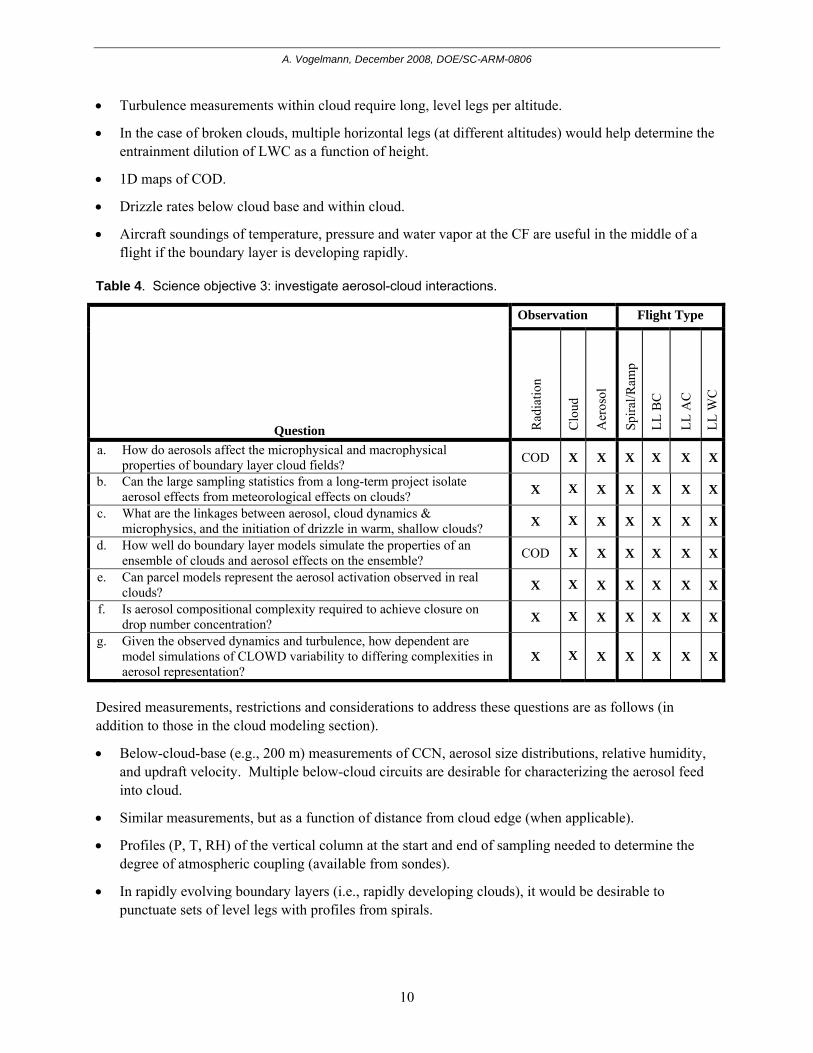
Table 4. Science objective 3: investigate aerosol-cloud interactions.
Question
Observation Flight Type
Rad
iatio
n
Clo
ud
Aer
osol
Spira
l/Ram
p
LL B
C
LL A
C
LL W
C
a. How do aerosols affect the microphysical and macrophysical properties of boundary layer cloud fields? COD X X X X X X
b. Can the large sampling statistics from a long-term project isolate aerosol effects from meteorological effects on clouds? X X X X X X X
c. What are the linkages between aerosol, cloud dynamics & microphysics, and the initiation of drizzle in warm, shallow clouds? X X X X X X X
d. How well do boundary layer models simulate the properties of an ensemble of clouds and aerosol effects on the ensemble? COD X X X X X X
e. Can parcel models represent the aerosol activation observed in real clouds? X X X X X X X
f. Is aerosol compositional complexity required to achieve closure on drop number concentration? X X X X X X X
g. Given the observed dynamics and turbulence, how dependent are model simulations of CLOWD variability to differing complexities in aerosol representation?
X X X X X X X
Desired measurements, restrictions and considerations to address these questions are as follows (in addition to those in the cloud modeling section).
• Below-cloud-base (e.g., 200 m) measurements of CCN, aerosol size distributions, relative humidity, and updraft velocity. Multiple below-cloud circuits are desirable for characterizing the aerosol feed into cloud.
• Similar measurements, but as a function of distance from cloud edge (when applicable).
• Profiles (P, T, RH) of the vertical column at the start and end of sampling needed to determine the degree of atmospheric coupling (available from sondes).
• In rapidly evolving boundary layers (i.e., rapidly developing clouds), it would be desirable to punctuate sets of level legs with profiles from spirals.

A. Vogelmann, December 2008, DOE/SC-ARM-0806
11
• Profiles of cloud LWC and Reff within the cloud using level legs, where the more vertical levels the better.
• 1D maps of COD.
• Drizzle rates below cloud base and within cloud.
• “Porpoising” flight patterns might be problematic for CCN measurements because the relative humidity changes quickly. However, this issue can be ameliorated limiting the ascent/descent to about 500 ft/s and/or accounting for pressure corrections.
Criteria for Measurement Success
To summarize, generally speaking the properties of greatest interest for the radiation, cloud and cloud-aerosol studies are as follows:
• Radiation PDFs of COD (from 1D mapping), Reff, and possibly cloud radiative forcing with adequate precision to distinguish PDFs for different cloud systems.
• Cloud PDFs of updrafts, COD and LWP (for more uniform clouds), and the height-dependence of LWC, Reff, and droplet number.
• Aerosol In addition to those given for clouds, we need PDFs of aerosol properties (e.g., accumulation mode number, median size), and CCN at different supersaturations.
Also needed are the linkages among all the PDFs (i.e., joint PDFs). After a given flight, we will analyze the raw data for critical properties (e.g., LWC, updraft velocity, etc.) to determine whether our PDFs are capturing the observed variability as necessary to address our science questions. If we are not, we will need to make adjustments to improve our sampling.
6. Sampling Strategy
Based on the sampling needs indicated in the previous section, we discuss an optimum flight strategy for obtaining relevant data to address the scientific questions. To enable RACORO to operate as a routine, long-term program, flight plans must be kept as simple and generic as possible to achieve its objectives, which cannot be biased by flight-day perceptions of what clouds are most scientifically interesting or most amenable to a simple sampling strategy. Unlike conventional aircraft campaigns that can have involved pre-flight discussions, RACORO discussions will be minimal and used only to make a go/no-go decision and, if we go, choose the flight pattern from a predetermined matrix. The flight plans are discussed here for three sets of cases: daytime cloud flights, nighttime cloud flights, and daytime clear-sky flights (needed for radiometer characterization and surface albedo measurements).
To assist these discussions, we summarize the types of cloud systems we anticipate. The summaries are based on the National Weather Service (NWS) cloud classifications that constitute the low-level CLOWD types. The descriptions of the cloud types are summarized in Table 5, and the corresponding cloud classifications are categorized in Table 6.

A. Vogelmann, December 2008, DOE/SC-ARM-0806
12
Since this is the first attempt at conducting routine AVP cloud-sampling flights, modifications may be needed to respond to unforeseen needs as they arise. This may include aspects of the flight plans including the overall schedule and timing of the flights, the order of the flight legs discussed here, and even the flight patterns used.
Table 5. National Weather Service CLOWD types. Seven low-level NWS cloud classifications are given that are CLOWDs. Information and cloud images obtained from the NWS Jetstream Max Project, http://www.srh.noaa.gov/jetstream/synoptic/l1.htm, and from http://www.srh.noaa.gov/key/HTML/galleries/Jim_Clouds/clouds.html.
Cloud Code Description Comment Sample Image
L1 Cumulus (Cu) with little vertical extent Clouds possibly too thin for aircraft penetrations at multiple within cloud heights (if cloud fraction large enough to fly).
L2 Cumulus (Cu) of moderate/strong development, which includes fair weather cumulus or cumulus humilis.
Aircraft penetrations at multiple within cloud heights cloud are likely, but spirals may not be able to stay within cloud.
L4 Stratocumulus (Sc) from spreading out of Cumulus (Cu)
NA
L5 Stratocumulus (Sc) not from spreading out of Cumulus (Cu)
NA
L6 Stratus (St) If deck is too thin, ramps are more effective than spirals for within cloud profiles.
L7 Stratus fractus (StFra) and/or Cumulus fractus (CuFra) bad weather
Avoid if there is wide spread precipitation in the area.
L8 Cumulus (Cu) and Stratocumulus (Sc) at different heights
Multiple cloud types and cloud heights within the field (i.e., very large degree of variability)

A. Vogelmann, December 2008, DOE/SC-ARM-0806
13
Table 6. Cloud structure categorization, based on Table 5 cloud classifications.
Mostly single-layered clouds Inhomogeneous cloud types and/or
Multi-layered Broken (cu) Patchy3 Plane-Parallel (St)
Thin2 L1 L4, L5 L6 L7, L8
Thick1 L2 L4, L5 L6 L7, L8 1 “Thick” clouds have sufficient vertical development (e.g., 500m or more) where three well-separated (vertically) penetration
legs are possible (e.g., bottom, middle, and top each separated by 100-200m). 2 “Thin” clouds are anything that are not “thick.”
3 Special patchy cloud cases are when they are organized (e.g., cloud streets).
6.1 Daytime Cloud Flights
Based on the sampling needs given in Section 5, the flight patterns need to include several components including profiles (via spirals or ramped ascents/descents) and level flight legs below, above and within the cloud. The optimal specifications for these components depend slightly on the cloud type encountered (e.g., Table 5). A general flight plan is first discussed that contains a baseline set of components needed to obtain the measurements needed, which is followed by comments on how the flight pattern would be fine-tuned based on the type of cloud system encountered on a given day.
The general flight plan is shown in Figure 2 and Figure 3 and consists of the following components:
1. Ferry flight from Guthrie (or Ponca) to the CF. We wish to obtain data during ferry flights (about 20 minutes each direction). One pattern that may be flown is starting the flight about 150 m below the boundary layer (BL) cloud bottom. (We prefer to keep a minimum separation for aerosol sampling and COD mapping.) After a time, ramp up through the cloud and fly about 150 m above the BL cloud top. Before reaching the SGP, ramp down below cloud bottom and fly at that level for about 5 minutes (to adjust the radiometer domes to ambient temperature).
2. Once at the CF, fly a triangular circuit about 150 m below cloud base using straight, level legs that are 20-45 km long (leg #1 in Figure 2) where one of the side legs runs along the wind and over the CF. The triangle must generally be positioned east of the CF to avoid the restricted airspace to the west.
3. Perform a profile ascent (spiral or ramp) through the depth of the cloud over the CF (leg #2) to obtain an in situ profile of cloud microphysical properties. Should a cloud not exist over the CF at that time, the ascent will be flown through a nearby, representative cloud that is either upwind or downwind from the CF (i.e., avoiding the restricted airspace to the west).
4. Fly a triangular circuit (leg #3) about 150 m above the median BL cloud-top height (possibly the altitude where the profile ascent exited cloud).
5. Step down in altitude by 100-200 m and fly another level leg triangle. The distance used for the downward step should be based on the best estimate of median cloud-top height such that approximately three in-cloud transects are made towards the top, middle and bottom of the cloud (legs #4, 5, 6).

A. Vogelmann, December 2008, DOE/SC-ARM-0806
14
6. Complete the sampling with an in-cloud profile ascent (leg #7) in the vicinity of the CF (as stipulated in Step 3).
7. Ferry flight back to Guthrie (or Ponca); pattern similar to that in step 1.
Figure 2. Triangular flight circuits. This is one possible pattern that will be used during RACORO. Other potential flight configurations may include (but are not restricted to) boxes, bow ties and “L”s. Here a green circle (●) indicates the SGP Central Facility (CF), a yellow arrow indicates direction of flight circuit, and circles at the triangle vertices indicate turns. The orientation of the pattern is oriented to the wind direction and may be flipped (dotted line) contingent on cloud conditions or flight obstacles.
Figure 3. General plan flight levels. This figure provides a qualitative view of a general flight pattern we envision for RACORO. Actual flight altitudes and patterns may be changed from those shown based on cloud conditions and improvements to our sampling strategies. This may include changing the order of the flight legs or introducing new flight configurations as needed.
A. Vogelmann, December 2008, DOE/SC-ARM-0806
15
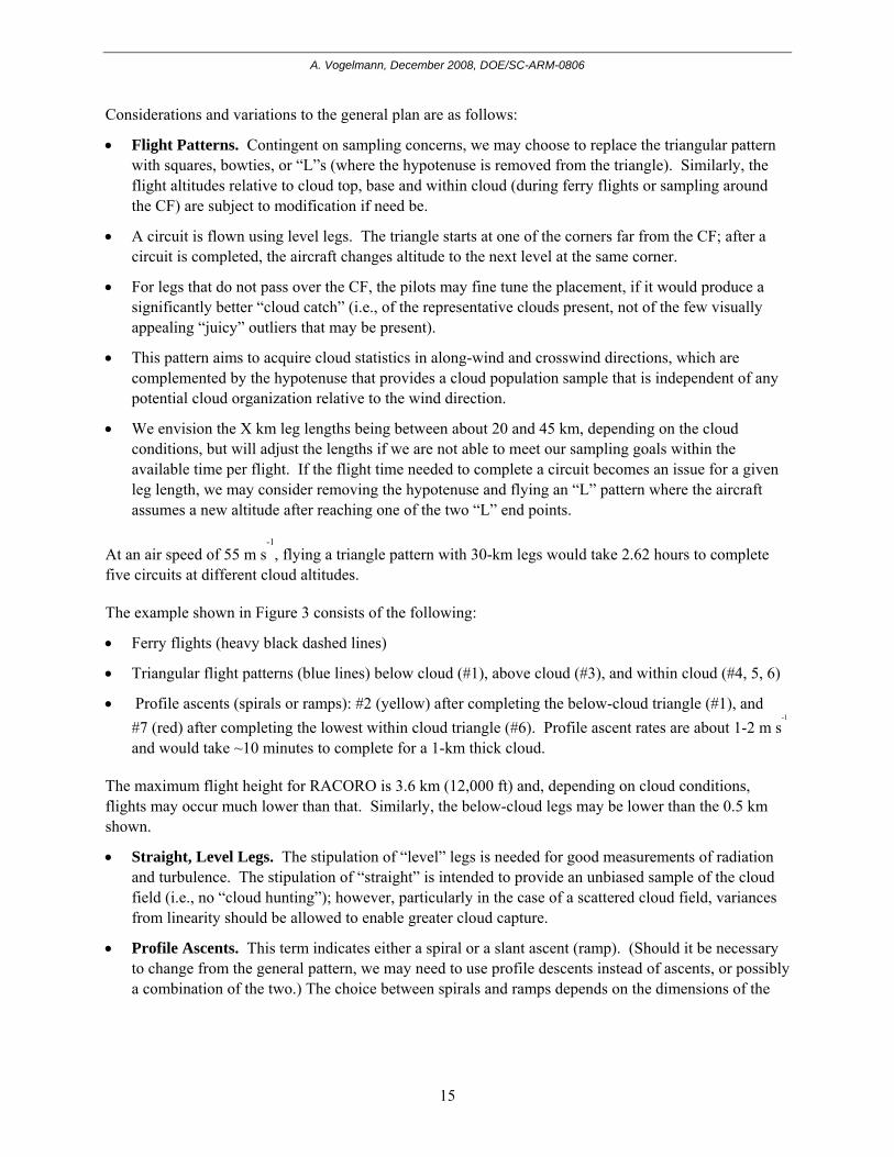
Considerations and variations to the general plan are as follows:
• Flight Patterns. Contingent on sampling concerns, we may choose to replace the triangular pattern with squares, bowties, or “L”s (where the hypotenuse is removed from the triangle). Similarly, the flight altitudes relative to cloud top, base and within cloud (during ferry flights or sampling around the CF) are subject to modification if need be.
• A circuit is flown using level legs. The triangle starts at one of the corners far from the CF; after a circuit is completed, the aircraft changes altitude to the next level at the same corner.
• For legs that do not pass over the CF, the pilots may fine tune the placement, if it would produce a significantly better “cloud catch” (i.e., of the representative clouds present, not of the few visually appealing “juicy” outliers that may be present).
• This pattern aims to acquire cloud statistics in along-wind and crosswind directions, which are complemented by the hypotenuse that provides a cloud population sample that is independent of any potential cloud organization relative to the wind direction.
• We envision the X km leg lengths being between about 20 and 45 km, depending on the cloud conditions, but will adjust the lengths if we are not able to meet our sampling goals within the available time per flight. If the flight time needed to complete a circuit becomes an issue for a given leg length, we may consider removing the hypotenuse and flying an “L” pattern where the aircraft assumes a new altitude after reaching one of the two “L” end points.
At an air speed of 55 m s-1, flying a triangle pattern with 30-km legs would take 2.62 hours to complete
five circuits at different cloud altitudes.
The example shown in Figure 3 consists of the following:
• Ferry flights (heavy black dashed lines)
• Triangular flight patterns (blue lines) below cloud (#1), above cloud (#3), and within cloud (#4, 5, 6)
• Profile ascents (spirals or ramps): #2 (yellow) after completing the below-cloud triangle (#1), and #7 (red) after completing the lowest within cloud triangle (#6). Profile ascent rates are about 1-2 m s
-1
and would take ~10 minutes to complete for a 1-km thick cloud.
The maximum flight height for RACORO is 3.6 km (12,000 ft) and, depending on cloud conditions, flights may occur much lower than that. Similarly, the below-cloud legs may be lower than the 0.5 km shown.
• Straight, Level Legs. The stipulation of “level” legs is needed for good measurements of radiation and turbulence. The stipulation of “straight” is intended to provide an unbiased sample of the cloud field (i.e., no “cloud hunting”); however, particularly in the case of a scattered cloud field, variances from linearity should be allowed to enable greater cloud capture.
• Profile Ascents. This term indicates either a spiral or a slant ascent (ramp). (Should it be necessary to change from the general pattern, we may need to use profile descents instead of ascents, or possibly a combination of the two.) The choice between spirals and ramps depends on the dimensions of the

A. Vogelmann, December 2008, DOE/SC-ARM-0806
16
cloud being sampled. Spirals will be used when the cloud has depth (e.g., > 250 m) and cloud diameter is sufficiently large that the aircraft can remain in cloud during the spiral (e.g., 5 km diameter). If either of these conditions is not met and the cloud diameter is still greater than 2 km, a ramp should be used. In the extreme case that the cloud diameter < 2 km and its thickness < 250 m (e.g., thin, small cumulus), the profile ascents should be skipped and the clouds sampled using only triangular circuits with level legs (the time saved could be used for longer flight legs needed to characterize the sparser cloud field). (See Table 7 for a summary of conditions.)
• Flight Leg Lengths. The length of the flight legs given in the general plan (i.e., “X” in Figure 1) will be designed to optimize the sampling for our science objectives, which affects the partitioning of available flight time between horizontal legs and profile ascents. Clearly, perspectives will differ depending on the measurement of interest (e.g., radiation, turbulence, aerosol, and cloud microphysics). Longer legs may be needed to capture the aerosol and radiation statistics when greater horizontal variability is present (aerosol, radiation, and updraft velocities). However, shorter legs might be used when we have more horizontally uniform cases (e.g., stratiform clouds), and put the time saved into more profile ascents. For example, for questions that require good turbulence measurements, level legs totaling at least 45 km may be needed per altitude level to capture the turbulent structure for cumulus; however, they might be as little as 30 km for stratus or stratocumulus. (See Table 7 for candidate lengths for different cloud conditions.)
Table 7. Summary of flight patterns and considerations. Provided are tentative choices, contingent on the cloud conditions, for the type of profile ascent and length of the triangular leg (“X” in Figure 1). Median cloud diameter is given by D and cloud thickness by H. All quantities in this table are approximations and will be modified as needed during the program.
Horizontal Cloud Dimension1 Approximate Leg
Length (km)
Type of Profile Ascent
Vertically developed (H > 250 m)
Thin (H < 250 m)
Large Clouds (D ≥ 5 km) 30 Spiral Ramp
Broken (2 ≤ D < 5 km) 35-40 Ramp Ramp
Scattered (D < 2 km) 45 None None 1 Diameters are approximate; 5 km is about the size needed for the pilot to keep the aircraft within a cloud during a spiral, and 2
km is about the lower limit for effective profile sampling by a ramp.
• Quickly Evolving Cloud Systems. In the event of a quickly evolving system, the general plan may need to be simplified. Such conditions could occur in a rapidly developing boundary layer (e.g., late morning flights) or a nighttime flight after sundown (discussed later). In these cases, we might consider a simplification of the general plan to enable faster sampling of the quickly evolving cloud state. This could be accommodated by modifications such as changing circuit pattern from a triangle to an “L” and/or reducing the number of in-cloud level leg transects. Also, in these cases, mid-way through the flight we may want to obtain atmospheric profiles (P, T, and RH) between the surface and cloud base.

A. Vogelmann, December 2008, DOE/SC-ARM-0806
17
• Pilot Discretion. We plan to attempt including approximately 30 minutes per flight to be used at pilot discretion. This block of time will accommodate potential delays from air traffic control, extra time needed to position the aircraft at a representative cloud downwind from the CF for profiling, and sonde launches (discussed later). Should such delays not occur, the time may be used for suggestions such as the following:
− Extra Triangles and Profile. After completing the general pattern (i.e., after step [6]), fly another above-cloud triangle, profile descend, and perform a below-cloud triangle. These end-of-flight samplings LL BC and LL AC would bookend the boundary conditions with the like-circuits done at the beginning (see Section 5 tables).
− Radiation Profile Descents. In addition to the “ramp ascents” described earlier, we may also want fly descending slant legs to measure radiative fluxes. These flights require a relatively homogenous cloud and that the plane's pitch is ≤ 2°. By adjusting the flap and power settings, the Twin Otter can descend at a rate between about 500 to 700 ft/min (can be between 300 to 1,000 ft/min) while maintaining the required pitch; so a 1,500-ft thick cloud (i.e., 0.5 km) would take between 3 and 2.2 minutes, respectively, to profile the cloud. This involves traversing a horizontal distance of about 10 to 6 km; so this option would need to be used along one of the X legs in Figure 1.
• Vertical Cloud Boundaries. The flight descriptions refer to cloud-top height and cloud-base height; however, they may be difficult to determine, especially for clouds that tend to be thin or tenuous. Such altitudes can vary within a cloud field over time and space. Further, it might be difficult even to identify a narrow altitude range to which clouds are confined. For this reason, a statistical approach is defined where cloud fields are sampled using long level legs. If enough level legs are flown at altitudes where clouds are expected to be present on a given day, the desired time in and below/above cloud will likely be obtained. This statistical sampling is particularly important for thin clouds or those that have highly variable tops (where a definitive determination of cloud boundaries is difficult to impossible) and the priority is for the aircraft to maintain a specific height above ground for a leg rather than a specific height relative to the cloud tops. Additional considerations are:
− Visually, pilots can tell whether they are in liquid cloud, and a tech onboard can tell from the FSSP or LWC data when they are in and out of cloud. Thus, the cloud top and base heights, identified from the initial profile ascent, can be used to select the altitudes for the later flight legs.
− Prior to take off, the pilots will have access to the quick look images from the prior 4-6 hours from the CF remote sensors, which will advise them about the vertical cloud boundaries they will likely encounter (but this is only an estimate since they vary a lot in time and space).
− Should difficulties and/or highly variable conditions warrant it, the surface meteorologist could radio in an update from the surface sensors.
− Profile ascents help resolve the cloud boundaries in the midst of this variability; however, too many are inadvisable, as they would come at the expense of obtaining other measurements needed to interpret cloud properties and dynamics (e.g., inputs at cloud base such as updraft velocity and aerosol size distributions, turbulence profiles within cloud from the level legs).

A. Vogelmann, December 2008, DOE/SC-ARM-0806
18
In the scenarios above, an on-board tech would be able to provide useful information from the real-time data feeds as to the locations of cloud boundaries. In addition, he/she could help troubleshoot the instrumentation as needed.
These are the basic considerations we anticipate using for the first flights. However we plan to revisit these issues carefully via discussions with the pilots and analysis of the raw data after the first few flights.
6.2 Nighttime Cloud Flights
We plan a limited number of nighttime flights for the purposes of validating retrieval algorithms, and obtaining cloud and cloud-aerosol nighttime observations. (These flights might also include time during twilight hours.) We envision a total of 8 flights that we prefer conducting (cloud conditions permitting) towards the beginning of the program when sunset occurs earlier and we are still on standard time (vs. daylight savings that starts 8 March). During this period, a departure from Guthrie about 7 PM CST would complete sampling just about the time of the Terra overpass (11:30 CST) and 0.5 hours before the sonde launch at midnight. The nighttime flights will prefer being held during the week of a full moon (full moon ±3 or 4 days), where the moonlight might assist flight execution (i.e., allow a visual of cloud top). Full moons occur during RACORO on 9 February, 11 March, 9 April, 9 May, and 7 June. The planned flight pattern will be similar to that used for the daytime flights, which will help the pilots’ execution through the familiarity gained during daytime flying. The IFR rules that would be used for the daytime in-cloud sampling will be similar to those at nighttime. However, modifications to the general flight plan may be necessary based on discussions with pilots and safety personnel.
6.3 Daytime Clear-Sky Flights
Clear-sky flights are needed for radiometer characterization and surface albedo measurements. Obtaining these measurements involves three types of patterns to be used at different points of the program, as described here and shown in Table 8.
1. Initial Radiometer Characterization
a. These tests must be done as early as possible to test the tilt correction methodology with the SPN-1, as well as the level of the radiometers with respect to the aircraft NAV data. The pattern can be flown at any height when the skies are cloud-free (hemispherically) above the aircraft. Potentially, they could be conducted by CIRPAS during the initial instrument test flights. The needed data are:
i. 20 minutes of straight-and-as-level-as-possible flight;
ii. 20 minutes of deliberately tilted flight, with up to ±10° pitch and roll (but most within ±5° pitch and roll) for about 7 minutes each:
1. Roll=0 and varying pitch
2. Pitch=0 and varying roll
3. Some with both varying.

A. Vogelmann, December 2008, DOE/SC-ARM-0806
19
b. The initial radiometer characterization also includes the radiometer orientation characterization (#2), described next.
2. Radiometer Orientation Characterization
This pattern is to be flown as part of the initial radiometer characterization, once a month after that, and at the end. The flights are needed to characterize the offset of the radiometers from level with respect to the axes of the airplane. The flights use a “box” flight pattern in clear skies, which involves flying straight and level legs at constant altitude, ideally at a higher altitude. The first leg has a heading directly into the sun, followed by a 90° turn to port, the second leg has a heading that puts the sun directly off the starboard wing, followed by a 90° turn to port, the third leg has a heading that puts the sun directly aft, followed by a 90° turn to port, and the fourth leg has a heading that puts the sun directly off the port wing. Each leg is 3-5 minutes long, so the whole pattern takes about 20-25 minutes. (Similar information is desired during overcast conditions over the CF, but this should occur naturally during cloud sampling.)
3. SGP CF Radiometer Comparisons and Surface Albedo Mapping
The last pattern is for comparison to the ground radiometers at the SGP CF and can also provide useful information for mapping the surface albedo around the CF. This pattern should be flown at least very early in the program and at the end. On a clear-sky day, we will fly six level legs over the CF as low as possible. The legs will have a “pinwheel” configuration centered on the CF, consisting of six 30° wedges (spans 360°). Each leg is 20 km long, so there is 10 km on either side of the SGP.
Table 8. Summary of clear-sky flights.
Type When flown Description 1. Initial radiometer
characterization ASAP Requires about 40 mins with clear-skies
above aircraft. Can be done at any height or location.
2. Radiometer orientation characterization
With #1, monthly, and at the end of the program
Requires 25 mins under clear skies. Can be flown anywhere, ideally done at high altitude.
3. CF radiometer comparison and surface albedo mapping
At least at the beginning and the end of the program.
Requires about 40 mins. Must be flown over the CF under clear skies.
6.4 Flight Safety
Flying the aforementioned patterns requires a mix of in-cloud and clear-sky flights that are governed by different flight safety rules, as well as air traffic control at the time of the flight. Based on the information provided here, AVP is responsible for providing a flight safety document for RACORO operations. It will be based on this document and will be reviewed by two boards at the Pacific Northwest National Laboratory (PNNL). It is possible that proposed flight patterns proposed here would need to be modified for flight safety. Only after approval from both boards can RACORO flights begin.

A. Vogelmann, December 2008, DOE/SC-ARM-0806
20
7. Flight Scheduling and Execution
7.1 Flight Schedule
The total number of flight hours for RACORO is ~320 hours, of which about 300 are available for research flights after California-Oklahoma ferrying and integration flight testing. The 300 hours are partitioned equally through the January 22 to June 30 research period, or approximately 14 hours per week.
Flight departures are predetermined following a schedule designed to sample different aspects of the diurnal cycle. Our default flight days are: Saturday, Monday, and Wednesday, where Saturday represents a weekly minimum in Vance AFB flight activity. If conditions are not favorable for flying those days (i.e., no go), the following day becomes the candidate day (i.e., Sunday, Tuesday and Thursday/Friday).
The flight timing on a given day is predetermined and will be posted in a calendar format on the RACORO Wiki prior to the beginning of operations. The flight calendar will be generated to optimize our sampling over the diurnal cycle, occurrence of satellite overpasses, and lunar illumination conditions. The timing will be designed to complete a diurnal cycle sampling every 4-6 weeks and will obey FAA rules that permit pilots a maximum of 10 flight hours per day, and require 12 hours downtime between flights (including time on station). When possible, we will choose times at or close to satellite overpasses, when the satellite viewing conditions are favorable, so that the satellite observations can provide an overview of the cloud field being sampled. The closest daytime overpasses (in GMT) are approximately 17:30 for Terra, 19:30 for Aqua, and 20:00 for CloudSat/CALIPSO. A full table of overpass times during RACORO is given in Appendix A. During the RACORO period, we have made arrangements for MISR Local Mode data to be acquired on Terra flight overpass paths #28 and 29 (path #27 is committed to another region, but could be requested for special cases). During June, we plan to request ASTER data acquisition for the purposes of studying the small-scale cumulus that are more common then and augment the potential overflight activities being discussed with Rich Ferrare (NASA Langley, See Section 7.5). Aspects that will affect flight time preferences are:
1. Morning, which climatologically has maximum low-cloud occurrence and is when the Terra satellite overpasses
2. Noon, for optimal solar retrieval validation conditions
3. Early afternoon, for Aqua and A-Train satellite overpasses
4. Late afternoon, towards the end of the cloud daytime cycle
5. Nighttime sampling (early evening or early morning), when lunar illumination conditions are favorable (e.g., full moon ±3 to 4 days).
Note that flights must not be in the vicinity of the SGP when sondes are airborne. Sondes are launched at the SGP at 00, 06, 12, and 18Z. Sondes ascend at a rate of about 4.5 m/s, and will take 13.3 minutes to rise above our flight ceiling of 12,000 ft (3.6 km). Communications with SGP personnel will be needed to verify that a sonde launched close to overflight times proceeded without event (i.e., on time and no failures that called for a repeat launch).

A. Vogelmann, December 2008, DOE/SC-ARM-0806
21
7.2 Flight Holds
While this schedule will have been determined by balancing multiple considerations, there should be some flexibility to modify the planned takeoff time in advance, should there be a compelling reason based, for example, on aircraft or instrument status or possible impending weather factors. Such changes should be made at least the day before and communicated to the flight steering committee (defined in Section 8). Substantial takeoff delays (e.g., more than 1-2 hours later than the time established on the preceding day) will not be permitted.
Because of potential delays in flight departure times or execution (e.g., air traffic control), we may not be able to complete our 4.5-5 hour flight plan between the scheduled sonde launches. To avoid having the aircraft in the same airspace as a sonde, a holding pattern will be used that positions the aircraft a safe distance away from the CF. For execution, we need the following:
1. A holding pattern that can be safely conducted until the sonde rises above the CF airspace. Preferably, the pattern can make use of the time for sampling (e.g., fly a spiral in a cloud at one of the vertices). The pattern will be designed by AVP in consultation with CIRPAS, safety personnel, and the RSC.
2. A reliable command channel and communication path is needed to notify pilots when the sonde is airborne, and when it has left the airspace.
3. The filed flight plans must allow for such holds.
7.3 Go/No-Go Decision Making
The decision to fly or cancel will be made on the flight day about 1.5 hours before takeoff. Substantial take-off delays will not be permitted due to the cost of keeping a pilot available for the day. If a flight is cancelled, it will be rescheduled for the following day. If a rescheduled flight cannot be flown, the flight will be dropped from the rotation and the next regularly scheduled flight will be executed. Factors that would constitute a no-go decision are:
1. Severe weather or icing conditions 2. Low-cloud cover is less than about 10%, and the RH at the top of the BL < 70% 3. Majority of low-cloud-top heights are greater than 3 km (our flight ceiling is 3.6 km)
4. Low cloud type is nimbostratus or cumulonimbus with wide-spread (synoptic-scale) precipitation.
Should a sequence of flights be dropped, the RSC may consider flying twice a day (observing the 10-hour daily flight maximum per pilot).
The go/no-go decision may also consider readiness of critical instruments (aircraft and surface). Such instruments are listed in Table 9, and would be at issue if the flight steering committee (defined in Section 8.1) believed that the remaining instrument complement would be severely restricted in addressing our science questions. Should immediate attempts to repair the instrument fail (e.g., reset, etc.) and no immediate path is seen to resolve the issue, flights may continue at the discretion of the RSC. To enable this decision making, the flight steering committee will be briefed on instrument status during the go/no-go telecons.

A. Vogelmann, December 2008, DOE/SC-ARM-0806
22
Table 9. Critical instrumentation. Satisfactory operation of these instruments may be considered when making the go/no-go decision if our science questions cannot be addressed with the remaining complement.
Critical Aircraft Measurements Cloud Microphysics Liquid-water content (LWC)
Cloud drop size distribution from 3 to 640 μm (diameter) Radiation Uplooking hemispheric SW (pyranometer)
Uplooking total/diffuse SW (SPN-1) Downlooking hemispheric SW (pyranometer)
Aerosol Instruments Aerosol size distribution (need from the PCASP or DMA) Total CN CCN
Aircraft state True aircraft speed Aircraft geopositioning data (lat/long/alt/heading/pitch & roll)
Atmospheric state Temperature, water vapor concentrations, pressure Updraft velocity
Critical Surface Instruments AERI
MMCR MWR TSI
7.4 Flight Day Schedule of Events
The schedule of events for flight days is summarized below. The chain of command and individual duties are explained in the next section.
1. Flight briefing begins 1.75 hours before scheduled departure. Go/no-go items #1-4 are reviewed. (Participants involved in the decision are given in Section 8.1.)
2. Go/no-go decision made 1.5 hours before scheduled departure. If fly: 3. AVP representative or pilot files the flight plan. 4. Research flight is conducted. 5. Flight debriefing is started about an hour after landing (nighttime flight debriefing determined by
the flight team). (Participants involved in the decision are given in Section 8.1.) Discussion items include:
a. Conditions encountered b. Instrument status (aircraft and surface) c. Pilot feedback on the difficulties (or not). e.g.:
i. Flying parallel and perpendicular to the wind in a cloud field ii. Flight control issues
iii. Cloud patterns or occurrence (spatial and temporal) that were not anticipated. 6. Instrument and flight summaries are recorded on the RACORO Wiki. (Personnel responsibilities
are described in Section 8.2.)

A. Vogelmann, December 2008, DOE/SC-ARM-0806
23
7.5 Coordination with Other Field Programs
To maximize the impact of the RACORO datasets, the RSC will be open to coordinate, as appropriate, with field programs operating at the SGP. Such coordination cannot compromise the routine, statistical sampling goals of RACORO; however, in achieving our objectives there is a degree of flexibility within our flight planning and operations that can be exercised for the purposes of coordination without compromising RACORO goals (e.g., flight plan, flight timing and frequency). Such arrangements will be determined with the consent of the RSC and AVP officials in coordination with the PI of the other field program. At this time, we are aware of three programs to consider.
• Dr. Richard Ferrare (NASA Langley) will overfly the RACORO flights with the King Air B200 in June. The King Air will be equipped with the airborne High Spectral Resolution Lidar (HSRL) and the Research Scanning Polarimeter (RSP) instrument (PI, Brian Cairns, Columbia University/NASA-GISS). The HRSL is used to characterize clouds and aerosols (aerosol extinction, backscatter, spatial distribution and movement). The RSP is the precursor to the Aerosol Polarimetry Sensor instrument on the NASA Glory satellite, scheduled to be launched next year, and will provide additional information for aerosols (optical thickness, effective radius, refractive index) and clouds (optical depth, effective radius, LWP). Such information will provide an excellent complement to RACORO goals. The King Air deployment will be supported by funding external to RACORO.
• Dr. Dong Huang (BNL) will conduct an ACRF intensive observational period (IOP), "Ground-Based Cloud Tomography Experiment at the SGP," for a month starting in late April. Its objective is to test the theorized possibility of using a linear array of scanning microwave radiometers to retrieve profiles of cloud LWC. This is pioneering research that shares RACORO’s goal of improving cloud property retrievals, and RACORO observations could be used for validation with overflights of the array.
• Coordination to avoid airspace conflicts with the AVP ARM Airborne Carbon MEasurements (ARM-ACME), which is a multi-institution and multi-agency airborne study of atmospheric composition and carbon cycling led by Dr. Sebastien Biraud (LBL). Cessna flights will occur about weekly over the SGP and will generally be chosen to provide cloud-free conditions, which provide the highest quality data from the ground-based OCO validation FTS system. A two-week IOP is also planned with daily CO2 profiles on days adjacent to the OCO overpass and 2-3 daily profiles during the overpass day.
8. Field Program Management
This section describes the chain of command and responsibilities of personnel involved in RACORO routine operations that include: the go/no-go decision telecon, flight debriefing telecon, and recording summaries of the flight conditions and operations. Modifications may be needed to respond to unforeseen needs as they arise.
8.1 Personnel Involved in Routine Operations
The RSC will operate on a rotating schedule where each will serve one week as a second in command, followed by one week as PI. The times for their rotations will be determined based on their availability and posted on the RACORO Wiki prior to the beginning of operations, along with their contact information. The respective managers from AVP and CIRPAS will determine rotation schedules for their key personnel and have their contact information posted on the Wiki.

A. Vogelmann, December 2008, DOE/SC-ARM-0806
24
On a candidate flight day, a go/no-go telecon briefing will be held about 1.75 hours prior to the planned take off time. The telecon requires the following participants, although other personnel directly involved in RACORO (e.g., pilots, scientists, etc.) are welcome to participate:
1. AVP representative
2. RSC PI
3. RSC second in command
4. SGP surface meteorologist.
These four people compose the “flight steering committee” for the day.
In the event of a flight, a debriefing telecon occurs about one hour after landing (timing at the discretion of the participants). The telecon requires the following participants:
1. AVP representative
2. RSC PI
3. RSC second in command
4. Pilot
5. CIRPAS technician.
8.2 Personnel Responsibilities
AVP Representative:
1. Makes the final go/no-go call based on input:
a. Scientific recommendation from RSC PI.
b. Their AVP operations recommendation (flight safety conditions, aircraft readiness).
2. Communicates the decision to pilot and, for flights, the flight pattern to be used.
3. Verifies that flight-day summaries are recorded on the Wiki (see reporting).
4. Tracks the flight time available and reports the balance on the Wiki after each flight (see reporting).
5. Supervises the timely availability of quick look aircraft data (described below).
RSC PI:
1. Makes the scientific go/no-go recommendation.
2. For flights:
a. Decides the flight pattern from the preset matrix
b. Reviews debriefing information and, if needed, makes scientifically based recommendations for modifications to preset plans.

A. Vogelmann, December 2008, DOE/SC-ARM-0806
25
RSC Second in Command:
1. Confers with PI on go/no-go decision, and on the flight plan to be used.
2. Serves as PI, if PI cannot assume responsibilities.
SGP Meteorologist:
1. For go/no-go telecons:
a. Serves as a cloud spotter who describes the current SGP cloud conditions.
b. Provides a nowcast of the cloud conditions based on the synoptic state.
c. Provides quick looks to the telecon participants (via the Wiki):
i. The most recent sonde launch and satellite image
ii. The prior 4-6 hours of data from the MMCR, MPL, Raman lidar, TSI, and MWR.
d. Reports on the readiness of critical SGP instrumentation (listed in Section 7).
2. For flights, provides the following postings on the Wiki:
a. A brief (e.g., 2 sentence) weather statement
b. A brief status of the monitored surface instruments (see Appendix B)
c. The quick look images provided in 1c.
Aircraft Technician:
Subject to AVP approval, the RSC recommends the following responsibilities.
1. Prior to flights
a. Wipes radiometer domes
b. Attends to other instrument needs as indicated by instrument PIs.
2. Takes notes about conditions encountered during flights and flight patterns flown and provides brief notes on the Wiki.
3. Provides brief aircraft instrument status report on the Wiki.
4. Provides cabin data to the IOP ftp share site.
9. Program Reporting and Information Dissemination
This section summarizes the reporting that will occur on a regular basis during operations. Modifications may be needed to respond to unforeseen needs as they arise.
A Wiki will be used to keep a running record of operations. The types of entries and ownership thereof are explained here.

A. Vogelmann, December 2008, DOE/SC-ARM-0806
26
1. Flight Days
a. SGP Meteorologist:
i. Weather statement
ii. Brief surface instrument status
iii. Quick look images (see Section 8.2).
b. CIRPAS Technician:
i. Notes about conditions encountered during flights and flight patterns flown
ii. Brief aircraft instrument status report.
2. Tracking Flight Progress The AVP representative (or designate) will be responsible for providing the following running summary of the flights:
a. Reports running flight hour balance
b. Provides brief tabulated summary that will include the days flown, when and hours in air, cloud type, pattern flown, etc.
10. Program Monitoring and Reviews
This section summarizes the monitoring and reviewing that will occur on a regular basis during operations and different intervals during RACORO. Modifications may be needed to respond to unforeseen needs as they arise.
10.1 Flight Day
The go/no-go decision-making review and flight debriefing are described in Section 8.1. Initial telecons may involve the full RSC for group consensus for go/no-go.
10.2 Weekly RSC Executive Board Telecons
The RSC executive board is a subset of the RSC with expertise in the critical areas (radiation, clouds, and aerosols). Board members will be posted on the Wiki prior to the beginning of operations. The executive board will monitor the following items in weekly telecons (more frequently at program start):
1. Review of field operations
2. Any data QA reports from the instrument PIs (standard monitoring)
3. Any available RSC science grade QA reports (focused science applications)
4. Discuss any practical issues that have arisen for the execution of operations
5. Review the Wiki summary records maintained by AVP (Section 9).

A. Vogelmann, December 2008, DOE/SC-ARM-0806
27
10.3 Mid-Program Review
This review will be held before the start of the March 2009 ARM Science Team Meeting (STM) and will include the following elements:
1. AVP operations summary
2. RSC science grade QA reports (focused science applications)
3. Review progress towards sampling objectives:
a. Flight plans: Investigate the statistical sampling confidence (e.g., 90% interval) of the different variables of interest for different cloud classes and/or meteorological states. Determine if our sampling strategy is lacking for a subset of the cloud types and modify it accordingly.
b. Instrumentation: Decide whether a different instrument is needed to measure a variable, or assess that, for unforeseen reasons, the needed accuracy cannot be attained in practice. If the latter, the instrument could even be replaced by another to focus on a different objective.
c. Achievement of sampling objectives: Should we determine that we are significantly ahead or behind our objectives, a plan modification may be made to best use the remaining time.
10.4 Final Program Review
A final program review will be held after the full completion of operations, which will include the following elements:
1. AVP operations summary
2. RSC science grade QA reports (focused science applications).
11. RACORO Data QC and Dissemination
In addition to the responsibilities given earlier for the execution of RACORO, this section details the needs and responsibilities relative to the data flow. A crucial product from RACORO is a dataset ready for science analysis and accomplishing this involves several levels of processing, quality control and reporting that AVP provide, as explained here. Since this is the first attempt of the AVP infrastructure at conducting routine flights, modifications may be needed to respond to unforeseen needs as they arise.
11.1 Immediate Processing and Reporting
Within 24 hours after each flight, the CIRPAS technician will provide the following:
1. Enter flight notes and status checklists/reports into flight database
2. Report on the Wiki 9 (1a) notes about conditions encountered during flights and flight patterns flown, and 9 (1b) brief aircraft instrument status report.

A. Vogelmann, December 2008, DOE/SC-ARM-0806
28
11.2 RACORO Instrument PI QC and Reporting
Preferably within 72 hours and definitely within 2 weeks after the receipt of data, the PIs are responsible for reviewing the data. Should any errors be found, they will be reported to a single AVP point of contact for dissemination to the rest of the team. Two weeks after flight, the PIs will put preliminary data on the IOP ftp share site.
11.3 Data Dissemination
The final data release will occur six months after the completion of operations (i.e., 1 January 2010).
1. Instrument PIs will put final data in the ACRF Data Archive.
2. AVP will make public the flight summaries and quick looks used, previously posted on the Wiki, to enable user data culling.
12. References
Bender, FA-M, H Rodhe, RJ Charlson, AML Ekman, and N Loeb. 2006. “22 views of the global albedo - comparison between 20 GCMs and two satellites.” Tellus-A 58 (3), 320-330, doi:10.1111/j.1600-0870.2006.00181.x.
Bony, S, and J-L Dufresne. 2005. “Marine boundary layer clouds at the heart of tropical cloud feedback uncertainties in climate models.” Geophysical Research Letters 32, L20806, doi:10.1029/2005 GL023851.
IPCC. 2007. Climate Change 2007: The Physical Science Basis. Contribution of Working Group I to the Fourth Assessment Report of the Intergovernmental Panel on Climate Change [Solomon, S., D. Qin, M. Manning, Z. Chen, M. Marquis, K.B. Averyt, M. Tignor and H.L. Miller (eds.)]. Cambridge University Press, Cambridge, United Kingdom and New York, NY, USA, 996 pp.
Lenderink, GA, P Siebesma, S Cheinet, S Irons, CG Jones, P Marquet, F Muller, D Olmeda, J Calvo, E Sanchez, and P Soares. 2004. “The diurnal cycle of shallow cumulus clouds over land: A single-column model intercomparison study.” Quarterly Journal of the Royal Meteorological Society 130, 33393364.
Sharon, TM, BA Albrecht, HH Jonsson, P Minnis, MM Khaiyer, TM van Reken, J Seinfeld, and R Flagan. 2006. “Aerosol and cloud microphysical characteristics of rifts and gradients in maritime stratocumulus clouds.” Journal of Atmospheric Science 63 (3), 983-997.
Stevens, B, G Vali, K Comstock, R Wood, MC van Zanten, PH Austin, CS Bretherton, and DH Lenschow. 2005. “Pockets of open cells (POCs) and drizzle in marine stratocumulus.” Bulletin of the American Meteorological Society 86, 51-57.

A. Vogelmann, December 2008, DOE/SC-ARM-0806
29
Turner, DD, SA Clough, JC Liljegren, EE Clothiaux, K Cady-Pereira, and KL Gaustad. 2006. “Retrieving liquid water path and precipitable water vapor from Atmospheric Radiation Measurement (ARM) microwave radiometers.” IEEE Transactions of Geoscience and Remote Sensing 45, 36803690, doi:10.1109/TGRS.2007.903703.
Turner, DD, AM Vogelmann, R Austin, JC Barnard, K Cady-Pereira, C Chiu, SA Clough, CJ Flynn, MM Khaiyer, JC Liljegren, K Johnson, B Lin, CN Long, A Marshak, SY Matrosov, SA McFarlane, MA Miller, Q Min, P Minnis, W O'Hirok, Z Wang, and W Wiscombe. 2007. “Thin liquid water clouds: Their importance and our challenge.” Bulletin of the American Meteorological Society 88, 177-190.
Twomey, S. 1974. “Pollution and the planetary albedo.” Atmospheric Environment 8, 1251-1256.
Zhang, MH, et al. 2005 “Comparing clouds and their seasonal variations in 10 atmospheric general circulation models with satellite measurements.” Journal of Geophysical Research 110, D15S02, doi:10.1029/2004JD005021.
Zhu, P, C Bretherton, M Kohler, A Cheng, A Chlond, Q Geng, P Austin, J-C Golaz, G Lenderink, A Lock, B Stevens. 2005. “Intercomparison and interpretation of single column model simulations of a nocturnal stratocumulus topped marine boundary layer.” Monthly Weather Review 133, 2741-2758.

A. Vogelmann, December 2008, DOE/SC-ARM-0806
30
Appendix A: Satellite Overpass Times
Tables A1-A3 provide daytime satellite overpass times during RACORO, which will be considered when establishing the predetermined flight times. All times are UTC. The current tabulation includes Terra and Aqua. Since CALIPSO and CloudSat will undergo orbital corrections in early January 2009, the information is not known at this time and will be added when available. The meanings of the times in the columns are as follows.
• MISR Local Mode
As discussed in Section 7.1, we have arranged to have MISR local mode data to be acquired on Terra flight overpass paths #28 and 29. These times are just a subset of the Terra overpass times.
• MISR
If MISR views the SGP region but not for path #28 or 29, the time is entered in the MISR column.
• Terra
When there is a Terra overpass when the peak satellite elevation is greater than 40° above the horizon (i.e., advantageous viewing geometry).
• Aqua
Aqua overpasses of the SGP when the peak satellite elevation is greater than 40° above the horizon.

A. Vogelmann, December 2008, DOE/SC-ARM-0806
31
Table A1. January and February
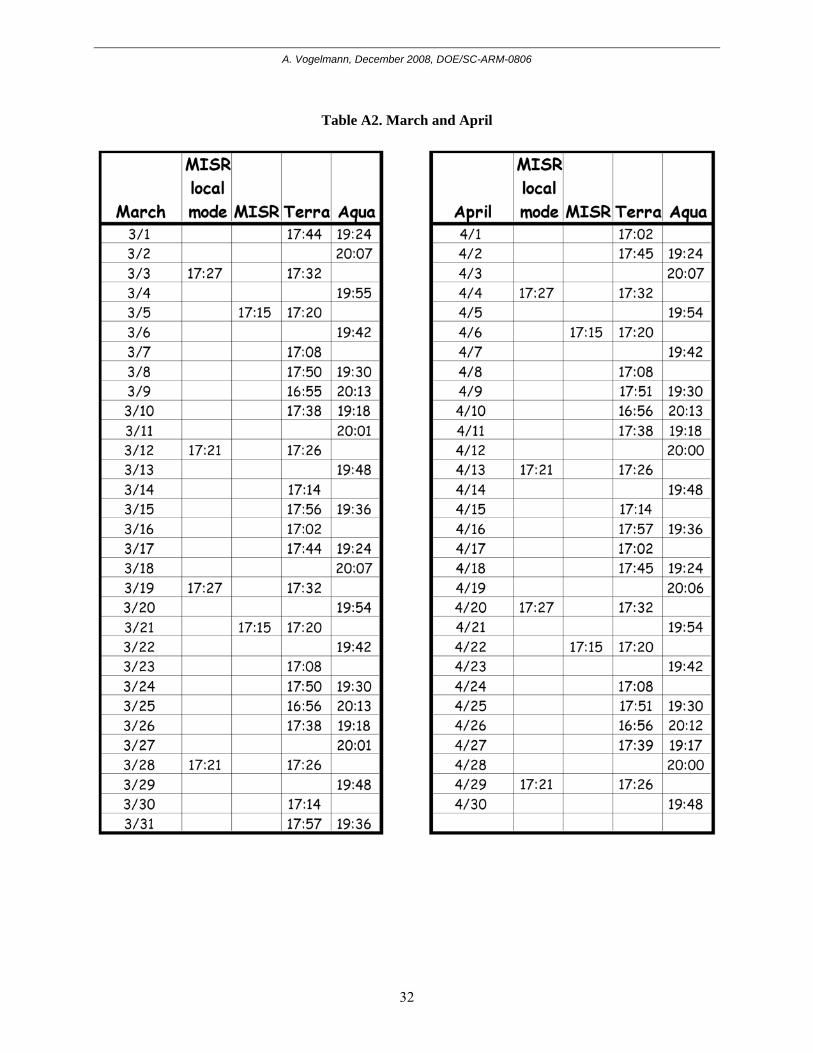
A. Vogelmann, December 2008, DOE/SC-ARM-0806
32
Table A2. March and April

A. Vogelmann, December 2008, DOE/SC-ARM-0806
33
Table A3. May and June

A. Vogelmann, December 2008, DOE/SC-ARM-0806
34
Appendix B: Monitored SGP CF Instrumentation
1. MMCR
2. S-WACR (when present)
3. AERI (rapid-sample mode)
4. MWRs (2 channel, and 3 channel when present)
5. MFRSR
6. Shortwave spectrometer
7. MPL
8. Raman lidar
9. Radiosondes
10. Shortwave broadband radiometers (pyranometers)
11. Longwave broadband radiometers (pyrgeometers)
12. TSI
13. Disdrometer
14. VCEIL
15. Surface aerosol properties
a. Size distribution (HTDMA, APS)
b. Number concentration (CN, CCN)
16. CIMEL
17. NIMFR
18. MWRP
19. 915 MHz wind profiler