radar range measurements in the...

SANDIA REPORT SAND2013-1096 Unlimited Release Printed February 2013

Radar Range Measurements in the Atmosphere

Armin W. Doerry

Prepared by Sandia National Laboratories Albuquerque, New Mexico 87185 and Livermore, California 94550

Sandia National Laboratories is a multi-program laboratory managed and operated by Sandia Corporation, a wholly owned subsidiary of Lockheed Martin Corporation, for the U.S. Department of Energy's National Nuclear Security Administration under contract DE-AC04-94AL85000.

Approved for public release; further dissemination unlimited.

- 2 -

Issued by Sandia National Laboratories, operated for the United States Department of Energy by Sandia Corporation.

NOTICE: This report was prepared as an account of work sponsored by an agency of the United States Government. Neither the United States Government, nor any agency thereof, nor any of their employees, nor any of their contractors, subcontractors, or their employees, make any warranty, express or implied, or assume any legal liability or responsibility for the accuracy, completeness, or usefulness of any information, apparatus, product, or process disclosed, or represent that its use would not infringe privately owned rights. Reference herein to any specific commercial product, process, or service by trade name, trademark, manufacturer, or otherwise, does not necessarily constitute or imply its endorsement, recommendation, or favoring by the United States Government, any agency thereof, or any of their contractors or subcontractors. The views and opinions expressed herein do not necessarily state or reflect those of the United States Government, any agency thereof, or any of their contractors.

Printed in the United States of America. This report has been reproduced directly from the best available copy.

Available to DOE and DOE contractors from

U.S. Department of Energy Office of Scientific and Technical Information P.O. Box 62 Oak Ridge, TN 37831 Telephone: (865) 576-8401 Facsimile: (865) 576-5728 E-Mail: [email protected] Online ordering: http://www.osti.gov/bridge

Available to the public from

U.S. Department of Commerce National Technical Information Service 5285 Port Royal Rd. Springfield, VA 22161 Telephone: (800) 553-6847 Facsimile: (703) 605-6900 E-Mail: [email protected] Online order: http://www.ntis.gov/help/ordermethods.asp?loc=7-4-0#online

- 3 -

SAND2013-1096 Unlimited Release

Printed February 2013

Radar Range Measurements in the Atmosphere

Armin W. Doerry ISR Mission Engineering

Sandia National Laboratories Albuquerque, NM 87185-0519

Abstract

The earth’s atmosphere affects the velocity of propagation of microwave signals. This imparts a range error to radar range measurements that assume the typical simplistic model for propagation velocity. This range error is a function of atmospheric constituents, such as water vapor, as well as the geometry of the radar data collection, notably altitude and range. Models are presented for calculating atmospheric effects on radar range measurements, and compared against more elaborate atmospheric models.

- 4 -

Acknowledgements

This production of this report is a result of an unfunded Internal Research and Development project.

- 5 -

Contents Foreword ............................................................................................................................. 6 1 Introduction & Background ......................................................................................... 7 2 Accounting for the Atmosphere .................................................................................. 9

2.1 Geometric Range ................................................................................................ 10 2.2 Propagation Path Range ..................................................................................... 12 2.3 Radar Range ....................................................................................................... 14 2.4 A Comparison of Ranges ................................................................................... 16 2.5 Finding the True Range from the Radar Range ................................................. 16 2.6 Effects of Unknown Refractivity ....................................................................... 19

3 Empirical Approximations ........................................................................................ 21 The Robertshaw Model ................................................................................................. 21

4 Model Approximations and Simplifications .............................................................. 25 4.1 Using Single Exponential Model for Refractivity .............................................. 25 4.2 Mean Index of Refraction .................................................................................. 27

5 Range Correction Strategies ...................................................................................... 31 5.1 Real-Time Correction ......................................................................................... 31 5.2 Post-Processing Correction ................................................................................ 31 5.3 Which is Best Strategy? ..................................................................................... 32

6 Conclusions ............................................................................................................... 33 Appendix A – Estimating Surface Refractivity ................................................................ 35

Absolute Temperature ................................................................................................... 35 Partial Pressure of Water Vapor ................................................................................... 36 Total Atmospheric Pressure .......................................................................................... 36 Putting it All Together .................................................................................................. 38 Exploring Some Numbers ............................................................................................. 39

References ......................................................................................................................... 45 Distribution ....................................................................................................................... 46

- 6 -

Foreword

This report details the results of an academic study. It does not presently exemplify any modes, methodologies, or techniques employed by any operational system known to the author.

The specific mathematics and algorithms presented herein do not bear any release restrictions or distribution limitations.

This distribution limitations of this report are in accordance with the classification guidance detailed in the memorandum “Classification Guidance Recommendations for Sandia Radar Testbed Research and Development”, DRAFT memorandum from Brett Remund (Deputy Director, RF Remote Sensing Systems, Electronic Systems Center) to Randy Bell (US Department of Energy, NA-22), February 23, 2004. Sandia has adopted this guidance where otherwise none has been given.

This report formalizes preexisting informal notes and other documentation on the subject matter herein.

- 7 -

1 Introduction & Background

A fundamental relationship that is the foundation for all radar is that a target’s range is proportional to an echo delay time. The actual relationship requires knowledge of the velocity of propagation of the signal whose echo delay time is measured. For a microwave signal, if we assume the propagation velocity is constant, the one-way time delay of a propagating signal is

c

rpathwayonedelay , , (1)

where

pathr = the path that the propagating signal takes, and

c = the actual (presumed constant) velocity of propagation over the path. (2)

For a monostatic radar, the total delay is a two-way delay, which is twice this. Consequently, for a monostatic radar

c

rpathdelay 2 . (3)

We repeat that an important premise for these equations is that the velocity of propagation along the path is in fact constant.

In radar, we frequently make the assumption that

truepath rr = the true geometric range, and

0cc = 2.99792458 × 108 m/s = speed of light in free space. (4)

We note that 0c is exact because the meter is in fact defined based on this velocity.

We then infer the true geometric range with the simplistic rule that

delaytruec

r 20 . (5)

However, this is only strictly true in free space. It is problematic that our radars typically operate in the un-free atmosphere. The question is “How much does the atmosphere interfere with calculating the ‘true range’ from propagation delay?”

The answer is “Somewhat.... It depends on how accurate you want to be.” For example, a radar operating at 25 kft altitude, and at 25 km range, might calculate range with an error of about 5 m based on the simplistic rule. Maybe this is good enough, and maybe it isn’t.

- 8 -

We can make some general comments at this point.

• The velocity of propagation in the atmosphere is always slower than in free space. This means that objects are really ‘closer’ than they appear when using the simplistic rule.

• The velocity of propagation decreases as dry air density increases, and also decreases as humidity increases.1,2 These things in fact vary with altitude and other factors. As a consequence, calculated range errors ensue.

This discussion often falls under the topic of “Atmospheric Refraction”, but more accurately is concerned with “Atmospheric Propagation”.

And finally we note that measuring time delay has its own issues. The radar typically measures time delay by counting cycles of some internal clock, which is designed to be accurate and precise, but does in fact exhibit its own errors. We will hereafter ignore time measurement issues, and assume that we can make time measurements with negligible error.

Additionally, we will assume perfect calibration of the radar, in that all internal time delays are precisely and accurately known and compensated.

A Note About Target Location Accuracy

The larger task is often to locate a target accurately and precisely with respect to an external geodetic datum (e.g. latitude, longitude, altitude). Radar inherently makes relative measurements, specifically of range. Angular direction measurements are made with Direction of Arrival (DOA) calculations, often using multiple range measurements from different perspectives. The ability to make absolute measurements relies on the ability of the radar to accurately and precisely know its own position, and even its own antenna orientation, neither of which are menial tasks.

Consequently, for accurate and precise target location, making accurate and precise range measurements alone are necessary, but not sufficient. In this report we will confine ourselves to the range measurement, and defer the larger target location problem to future reports.

- 9 -

2 Accounting for the Atmosphere

The following discussion addresses improvements to the accuracy and precision of range measurements; essentially when the simplistic rule isn’t good enough. We will generally assume a geometric optics model for propagation.

We will follow the analysis in a report by Robertshaw3 prepared for the Joint STARS project.

There are really three ranges to consider for this discussion. These are

truer = the true direct geometric distance from one point to another,

pathr = the true distance along the actual path of propagation, and

radarr = the radar simplistically calculated range. (6)

We observe that for a monostatic radar, the simplistic model is the calculation

delayradarc

r 20 , (7)

We also note that generally the various ranges are related by

radarpathtrue rrr , (8)

with strict equality holding only for free space. The difference between pathr and radarr

is strictly due to the slowed propagation velocity along that bent ray path. The difference between pathr and truer is due to ‘bending’ of the ray path itself.

What follows is an examination of these various ranges. We necessarily will make some assumptions that will allow us to engage this analysis, to wit

1. We shall assume a spherical earth. When a numerical earth radius is required, we will assume

eR = 6378 km = nominal earth radius. (9)

2. We will assume models(s) for atmospheric refractivity as detailed in an earlier report by this author.4

3. As a basis for comparison, we will equate the ground range, defined as the arc length along a constant earth radius between target and aircraft nadir.

- 10 -

2.1 Geometric Range

The geometric range is defined to be ‘truth’, and does not depend on electromagnetic propagation, or any associated refraction. We define the geometry with the parameters

hs = altitude of target surface, ha = altitude of aircraft,

truer = true geometric range from aircraft to surface target,

e = angular difference between aircraft and target from earth center, d = depression angle at aircraft (positive below horizontal), and g = grazing angle at target (positive above horizontal). (10)

These are illustrated in Figure 1.

Earth

Radar

Target

Re

Re

ha

hs

d

g

rtrue

e

Figure 1. Spherical earth geometry.

- 11 -

These parameters are related via the following set of equations, derived using the Law of Cosines for planar surfaces.

ae

true

ae

sa

true

sad hR

r

hR

hh

r

hh

22

1sin ,

se

true

se

sa

true

sag hR

r

hR

hh

r

hh

22

1sin , and

aese

satruee hRhR

hhr

2

1cos22

. (11)

Furthermore,

daesedaetrue hRhRhRr 222 cossin ,

222 2sinsin sasasegsegsetrue hhhhhRhRhRr , or

2cos12 saeaesetrue hhhRhRr . (12)

The arc length along the earth’s surface (assumed to be at the target altitude) between nadir and the target, is given by

ese hRd . (13)

Combining all this yields the ability to calculate geometric ‘slant range’ from ground range as

2cos12 sase

aesetrue hhhR

dhRhRr

. (14)

Example

We offer as example the following input geometry.

sh = 0,

ah = 10 kft = 3048 m, and

d = 100 km. (15)

From these input parameters we calculate (perhaps with excessive precision)

truer = 100069.297 m. (16)

- 12 -

2.2 Propagation Path Range

The propagation path range takes into consideration the bent ray path of propagation, due to atmospheric refraction. It does not consider effects of the speed of propagation otherwise. This range is independent of any time delays along the path.

From the earlier report we identify the calculation of the propagation path range as the line integral

dhdhra

s

a

s

h

h

h

hpath

2cos1

1

sin

1, (17)

where the instantaneous angle cosine is calculated from

h

shhd

hd

dn

n

e

seg e

hR

hR1

coscos . (18)

Herein we identify the refraction index as

Nn 6101 = index of refraction proper, and N = measure of refractivity in N-units. (19)

The index of refraction in the atmosphere (where relative permeability is inconsequential) is related to the relative permittivity, or dielectric constant as

rn , (20)

where

r = atmosphere relative dielectric constant. (21)

These are generally a function of altitude. Bean and Thayer5 offer a model of how refractivity changes with altitude. We write their segmented model’s dependence of refractivity on altitude as

- 13 -

kft 30m9000105

m9000m1000

m1000

7023

9000

m1000

1

he

hheN

hhhNhhN

hN

h

sH

hh

ssss

s

(22)

where

Ns = a measure of refractivity in N-units at the surface, N1 = a measure of refractivity in N-units at 1000 m above the surface,

N = refractivity linear decay constant in N-units per meter, and H = refractivity exponential decay constant in meters. (23)

Bean and Thayer offer that the refractivity decay constants can be calculated by

sNeN 005577.000732.0 , and

105ln

8000

1N

hH s . (24)

Simpler approximations to this model are offered in the earlier report. Across the continental US, the parameter sN ranges from about 250 in dry air to about 400 in

extremely humid air. It may be calculated from more conventional meteorological data, as is discussed in Appendix A. For completeness, we also identify

ss Nn 6101 = index of refraction at the surface. (25)

The ground range can be calculated as

dhhR

hRdh

hR

hRd

a

s

a

s

h

h e

seh

h e

se

2cos1

cos

tan

1. (26)

So, at this point we have the ability to calculate propagation path range pathr and ground

range d from an input target height hs, radar height ha, refractivity profile hN , and

grazing angle g . These calculations require an integration (perhaps numerical) of a

function of refractivity. What we would like instead is to start with ground range d instead of grazing angle g , and therefrom calculate propagation path range pathr . To

accomplish this, we offer the following strategy.

- 14 -

1. Use your favorite numerical technique to find the right grazing angle g to yield

the desired ground range d. Such a technique might be iterative. The nature of the relationship is conducive to gradient search techniques.

2. With the proper grazing angle identified, we may calculate the propagation path range pathr .

Example


sh = 0,

ah = 10 kft = 3048 m, and

d = 100 km. (27)

In addition, we will assume the segmented model of Bean and Thayer for refractivity versus height, with a surface refractivity of

Ns = 313 N-units. (28)

From these input parameters we calculate (again perhaps with excessive precision, but to make a point)

g = 1.4028 degrees, and

pathr = 100069.344 m. (29)

This differs from the true range by 4.7 cm, which is less than 1 ppm.

2.3 Radar Range

The radar range is calculated as proportional to the time delay of the radar signal along the propagation path. The constant of proportionality is an assumed propagation velocity. We will make the common assumption that the reference velocity of propagation is that in free space. Specifically, for a monostatic radar we identify

20 delay

radar

cr

, (30)

where

delay = the round-trip (two-way) echo delay time. (31)

- 15 -

Since the refractivity is a function of altitude, the actual velocity of propagation is also a function of altitude. Consequently, the time it takes the radar wavefront to propagate a fixed differential distance also is a function of altitude. Consequently, the round-trip echo delay time can be calculated as a weighted line integral

dhc

a

s

h

hdelay

2cos1

12 , (32)

where is a function of the index of refraction as previously given, and the velocity of propagation is also a function of the index of refraction as

n

cc 0 . (33)

Combining several of the previous equations yields

dhn

dhn

ra

s

a

s

h

h

h

hradar

2cos1sin. (34)

As before, we would like to start with ground range d instead of grazing angle g , and

therefrom calculate propagation path range pathr .

Example


sh = 0,

ah = 10 kft = 3048 m, and

d = 100 km. (35)

As before, we will assume the segmented model of Bean and Thayer for refractivity versus height, with a surface refractivity of

Ns = 313 N-units. (36)

From these input parameters we calculate

g = 1.4028 degrees, and

pathr = 100095.452 m. (37)

This differs from the true range by 26.154 m, or approximately 261 ppm.

- 16 -

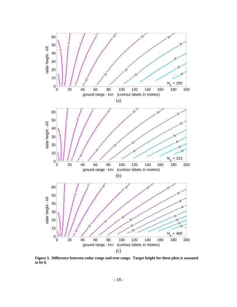
2.4 A Comparison of Ranges

We note from the previous analysis, and especially the examples, that the relative differences exhibit the characteristic

pathradartruepath rrrr . (38)

That is, the effect of the ‘bending’ the propagation path is much smaller than the effect of ‘slowing down’ the propagation velocity. This is consistent with the literature, which suggests that we may typically assume as a practical matter that

truepath rr . (39)

We explore this some more in the following plots.

Figure 2 shows the difference in pathr and truer , for a continental US average surface

refractivity of 313 N-units, for a rather dry surface refractivity of 250 N-units, and for a rather humid surface refractivity of 400 N-units.

Figure 3 shows the difference in radarr and truer , for a continental US average surface

refractivity of 313 N-units, for a rather dry surface refractivity of 250 N-units, and for a rather humid surface refractivity of 400 N-units.

Indeed, these plots show that for even somewhat extreme conditions (i.e. 200 km range, shallow grazing angles, humid atmosphere, etc.) the difference between propagation path range and true range is rarely greater than 1 m (5 ppm) or so, and is overwhelmed by the difference between radar range and true range.

2.5 Finding the True Range from the Radar Range

When all is said and done, the radar reports radarr , but we really want truer . So the task

at hand is to begin with radarr and calculate truer from it, based on knowledge (either real

or assumed) of the propagation characteristics.

Using the foregoing analysis, we propose the following general outline for accomplishing this with maximum precision and accuracy.

- 17 -

0.01

0.02

0.02

0.03

0.03

0.05

0.05

0.07

0.1

ground range - km (contour labels in meters)

rada

r he

ight

- k

ft

Ns = 250

0 20 40 60 80 100 120 140 160 180 2000

10

20

30

40

50

60

(a)

0.01

0.02

0.03

0.03

0.05

0.05

0.07

0.07

0.1

0.1

0.2

0.3


rada

r he

ight

- k

ft

Ns = 313

0 20 40 60 80 100 120 140 160 180 2000

10

20

30

40

50

60

(b)

0.01

0.02

0.02

0.03

0.03

0.05

0.05

0.07

0.07

0.1

0.1

0.2

0.2

0.3

0.5

0.7


rada

r he

ight

- k

ft

Ns = 400

0 20 40 60 80 100 120 140 160 180 2000

10

20

30

40

50

60

(c)

Figure 2. Difference between propagation path range and true range. Target height for these plots is assumed to be 0.

- 18 -

12

3 5

7

7

10

10

15

15

20

20

25

25

30

35

40


rada

r he

ight

- k

ft

Ns = 250

0 20 40 60 80 100 120 140 160 180 2000

10

20

30

40

50

60

(a)

12

3 5

7

7

10

10

15

15

20

20

25

25

30

30

35

40

45

50


rada

r he

ight

- k

ft

Ns = 313

0 20 40 60 80 100 120 140 160 180 2000

10

20

30

40

50

60

(b) 1

2

3 5

7

7

10

10

15

15

20

20

25

25

30

30

35

35

40

40

45

50

5560


rada

r he

ight

- k

ft

Ns = 400

0 20 40 60 80 100 120 140 160 180 2000

10

20

30

40

50

60

(c)

Figure 3. Difference between radar range and true range. Target height for these plots is assumed to be 0.

- 19 -

1. We shall assume as input to this process the aircraft/radar altitude ah , the target

altitude sh , the measured radar range radarr , and a model for the refractivity as a

function of altitude N(h).

2. Use your favorite numerical technique to find the right grazing angle g to yield

the measured radar range radarr . Such a technique might be iterative. The nature

of the relationship is conducive to gradient search techniques.

3. With the proper grazing angle identified, we may calculate the ground range d . This is also likely a numerical integration.

4. From the ground range d, we may now calculate the true geometric range truer .

We stipulate that this is a rather cumbersome procedure. Hence, we desire something simpler to implement, but still with adequate precision and accuracy.

Ideally, we wish to find an easily calculable function that lets us calculate truer from

radarr . We generically write this as

radarcorrecttrue rfr . (40)

The principal goal of this report is to develop and/or present suitably simpler, but still adequate, functions radarcorrect rf . The preference would be something that doesn’t

involve numerical integrations and iterative techniques.

2.6 Effects of Unknown Refractivity

An important question is “What if we guess wrong on surface refractivity?” Clearly this should yield errors in our calculation of true range from the measured radar range.

We present as example several plots where the radar range was calculated using some ‘true’ value, but the estimated true range was calculated based on an ‘assumed’ nominal value for surface refractivity. In all cases, the segmented refractivity model of Bean and Thayer was used. Figure 4 uses a reference value of 313 N-units for extreme true values. Figure 5 uses an assumed value within 25 N-units of a true extreme value of 400 N-units.

A simplistic heuristic rule-of-thumb might be that at 25 kft, a surface refractivity error of 25 N-units will account for approximately 10 ppm error. This would be roughly doubled at 5 kft.

- 20 -

-5

-5

-2

-2

-2

-1

-1

-0.5

-0.5

-0.2


rada

r he

ight

- k

ft

Ns = 250 (true), 313 (assumed)

0 20 40 60 80 100 120 140 160 180 2000

10

20

30

40

50

60

(a)

0.5

0.5

1

1

2

2

2

5

5

10


rada

r he

ight

- k

ft


0 20 40 60 80 100 120 140 160 180 2000

10

20

30

40

50

60

(b)

Figure 4. True range estimation error due to using inaccurate surface refractivity.

0.1

0.1

0.2

0.2

0.5

0.5

1

1

1

2

2


rada

r he

ight

- k

ft


0 20 40 60 80 100 120 140 160 180 2000

10

20

30

40

50

60

Figure 5. True range estimation error due to using inaccurate surface refractivity.

- 21 -

3 Empirical Approximations

We offer next an empirical model from the literature.

The Robertshaw Model

A report by Robertshaw3 in support of the Joint STARS program derived an empirical relationship that can be manipulated to the expression

1

1

kft

sradartrue h

NBArr . (41)

where

A = 0.42 m, B

= 0.0577 × 103 (kft/N-unit)0.5,

kfth = radar altitude in kft,

sN = measure of surface refractivity. (42)

We note that the sign on the constant A is different than in the Robertshaw report. This is necessary to make this model consistent with his tabulated results.

This model was designed to match a higher-fidelity simulation (based on a MITRE ray-trace method using the Bean and Thayer segmented model) for altitudes from 15 kft to 65 kft, for ranges from 40 km to 200 km, and a target height of 1 kft. This model, along with ‘truth’ points provided by Robertshaw, is shown in Figure 6. Robertshaw’s model matches his truth points with an RMS error of 1.42 m. This is actually quite good for as simple a model it is.

0 20 40 60 80 100 120 140 160 180 2000

10

20

30

40

50

60

range - km

rang

e er

ror

- m

15 kft - blue35 kft - magenta45 kft - green65 kft - red

Figure 6. Solid lines represent the Robertshaw model, whereas asterisks represent ‘truth’ data. Each color quartet represents Ns values of 250, 300, 350, and 400 N-units.

- 22 -

Several points are worth stressing.

• Data from Robertshaw’s report shows mean values for surface refractivity are in the range of 330 with a standard deviation in the range of 20 or so. Although this is slightly more humid than the continental US average of 313, it is nevertheless still pretty close.

• It is important to remember that this empirical relationship is derived from data calculated from the Bean and Thayer segmented model, but over a limited set of altitudes, a limited set of ranges, and one specific target height. Over this parameter space there seems to be a relatively good fit. There is no indication of utility outside this parameter space, although some obvious problems exist.

• Most models tend to assume (this one included) horizontally stratified layers (or at least parallel to the earth’s surface), and neglects inversion situations and horizontal gradients. Usually this seems to work pretty well. Places where this does tend to be a little off is near water/land boundaries, especially where dry desert air meets humid ocean air, like the coastal regions of the Persian Gulf.

• In this simplified model, and consistent with truth data, what makes things worse are 1) lower altitudes, and 2) more humidity.

In any case, combining some equations lets us write

radaravg

true rc

cr

0

, (43)

where we estimate an approximate average velocity of propagation as

1

0 1

h

NB

r

Acc s

trueavg , (44)

which is reasonably good over Robertshaw’s report’s parameter space. This is plotted in Figure 7. One problem is that at some parameter combinations, this allows a velocity of propagation that exceeds that of free space. Consequently, a reasonable modification might be

1

00 1,minh

NB

r

Accc s

trueavg , (45)

Note that the average velocity of propagation seems to behave undesirably at the shorter ranges, where a number of short and medium range radar systems often are employed. Using this model gives a range correction as indicated in Figure 8.

- 23 -

Another question is “How well does the Robertshaw model compare with the true range estimate from the previous section using our numerical integration of the Bean & Thayer model?” To answer this, we offer the range error plots in Figure 9. We observe that at altitudes above 15 kft, and ranges beyond 40 km, the difference tends to be less than a couple of meters or so for nominal surface refractivity, comparing favorably with the errors displayed in Figure 6. The differences may be somewhat more for some extreme surface refractivity as also illustrated in Figure 9. We observe, however, that for all cases below 15 kft, the differences grow rather large, even at relatively short ranges.

Joint STARS notwithstanding, many ISR radar sensors do in fact operate at lower altitudes, and at the ranges precisely where this particular empirical model exhibits some difficulties.

While the Robertshaw model is relatively easy to calculate, nevertheless a reasonable question is “Is there a better model for the larger parameter space?” The answer is “Better models exist at the price of a little more complexity.”

0 20 40 60 80 100 120 140 160 180 200

2.9965

2.997

2.9975

2.998x 10

8

c0

range - kmmea

n ve

loci

ty o

f pr

opag

atio

n -

m/s

65554535

25

15

5

Ns = 330

Figure 7. Velocity of propagation vs. range from the Robertshaw empirical model with Ns = 330, and altitude labels in kft. Solid lines denote valid parameter space for the model.

0 20 40 60 80 100 120 140 160 180 2000

20

40

60

80

100

range - km

calc

ulat

ed r

ange

cor

rect

ion

- m

655545352515

5

Ns = 330

Figure 8. Calculated range correction vs. range and altitude from the Robertshaw empirical model with Ns = 330, and altitude labels in kft. Solid lines denote valid parameter space for the model.

- 24 -

-20-20-10

-10

-5

-5-5

-2

-2 -2

-1

-1 -1

-0.5

-0.5 -0.5

-0.2-0.2

-0.2

-0.2 -0.2

-0.1-0.1

-0.1

-0.1-0.1

-0.05-0.05

-0.0

5

-0.05-0.05

-0.02-0.02

-0.0

2

-0.02-0.02

-0.01-0.01

-0.0

1

-0.01-0.01

00

0

00

0.010.01

0.01

0.010.01

0.020.02

0.02

0.020.02

0.050.05

0.05

0.050.05

0.1

0.1

0.1

0.10.1

0.2

0.2

0.2

0.2

0.20.2

0.5

0.5

0.5

1

1


rada

r he

ight

- k

ft


0 20 40 60 80 100 120 140 160 180 2000

10

20

30

40

50

60

(a)

-20-20

-10

-10-5

-5 -5

-2

-2 -2

-1

-1 -1

-0.5 -0.5

-0.5

-0.5 -0.5

-0.2-0.2

-0.2

-0.2 -0.2

-0.1-0.1

-0.1

-0.1-0.1

-0.05-0.05

-0.05

-0.05-0.05

-0.02-0.02

-0.02

-0.02-0.02

-0.01-0.01

-0.01

-0.01-0.01

0

0

0

0

00

0.010.01

0.01

0.010.01

0.020.02

0.02

0.020.02

0.05

0.05

0.050.05

0.05

0.1

0.1

0.1

0.10.1

0.1

0.2

0.2

0.2

0.20.2

0.2

0.5

0.5

0.5

0.5

1

1

2


rada

r he

ight

- k

ft


0 20 40 60 80 100 120 140 160 180 2000

10

20

30

40

50

60

(b)

-20

-10

-10

-5-5

-5-2

-2 -2

-1 -1

-1

-1-1

-0.5 -0.5

-0.5

-0.5 -0.5

-0.2-0.2

-0.2-0.2 -0.2

-0.1-0.1

-0.1-0.1

-0.1

-0.05-0.05

-0.05-0.05

-0.05

-0.02-0.02

-0.02-0.02

-0.02

-0.01

-0.01

-0.01-0.01

-0.01

0

0

0

00

0

0.01

0.01

0.01

0.010.01

0.01

0.02

0.02

0.02

0.020.02

0.02

0.05

0.05

0.05

0.050.05

0.05

0.1

0.1

0.1

0.10.1

0.1

0.2

0.2

0.2

0.2 0.20.2

0.5

0.5

0.5

0.50.5

1

1

1

2

2


rada

r he

ight

- k

ft


0 20 40 60 80 100 120 140 160 180 2000

10

20

30

40

50

60

(c)

Figure 9. True range estimation error of the Robertshaw model compared to numerical integration of the segmented Bean and Thayer model. Target height for these plots is assumed to be 0.

- 25 -

4 Model Approximations and Simplifications

We now examine some simplifications to the numerical techniques of the first section.

4.1 Using Single Exponential Model for Refractivity

We now use essentially the technique outlined in Section 2.5 except that we will use a single exponential model for the refractivity as a function of altitude, instead of using the segmented Bean and Thayer model. Specifically, we will assume

b

s

H

hh

s eNhN

, (46)

where

b

s

sbb

N

N

hhH

ln

. (47)

We will presume that our interest is principally over an altitude range of 0 to 50 kft, so we might choose

m 12192 kft 40 bh , and

65.66bN N-units. (48)

This lets us calculate the instantaneous depression angle as a function of altitude as the closed form expression

hR

hR

eN

N

e

se

H

hh

s

sg

b

s

6

6

101

101coscos . (49)

Otherwise we are still using iterative techniques to find the grazing angle, and numerical integration to find ground distance d.

Figure 10 details the error of this model compared to the Bean and Thayer segmented mode. We observe that even for worst case humid air, the error is less than 1 m out to 100 km ground range, and less than 2 m out to 200 km ground range, over the entire 0 to 65 kft altitude range.

The point of all this is to show that the single exponential model for refractivity works reasonably well, contributing no more than 10 ppm error even for worst case conditions.

- 26 -

-0.2-0.1-0.1

-0.05

-0.05-0.05

-0.0

2

-0.02 -0.02

-0.01-0.01 -0.010 0 00.01 0.01 0.01

0.02 0.02 0.02

0.05

0.05

0.05 0.05

0.1

0.1

0.1 0.1

0.2

0.2

0.2 0.2

0.5

0.5

0.5


rada

r he

ight

- k

ft


0 20 40 60 80 100 120 140 160 180 2000

10

20

30

40

50

60

(a)

-0.2

-0.2

-0.1

-0.1-0.1

-0.05

-0.05-0.05

-0.0

2

-0.02-0.02

-0.01-0.01 -0.010 0

0

0.01

0.01 0.01 0.01

0.02

0.020.02 0.02

0.05

0.05

0.05 0.05

0.1

0.1

0.1 0.1

0.2

0.2


rada

r he

ight

- k

ft


0 20 40 60 80 100 120 140 160 180 2000

10

20

30

40

50

60

(b)

-1

-1

-0.5

-0.5

-0.5

-0.2

-0.2

-0.1

-0.1

-0.05


rada

r he

ight

- k

ft


0 20 40 60 80 100 120 140 160 180 2000

10

20

30

40

50

60

(c)

Figure 10. True range estimation error of the single exponential model compared to numerical integration of the segmented Bean and Thayer model. Target height for these plots is assumed to be 0.

- 27 -

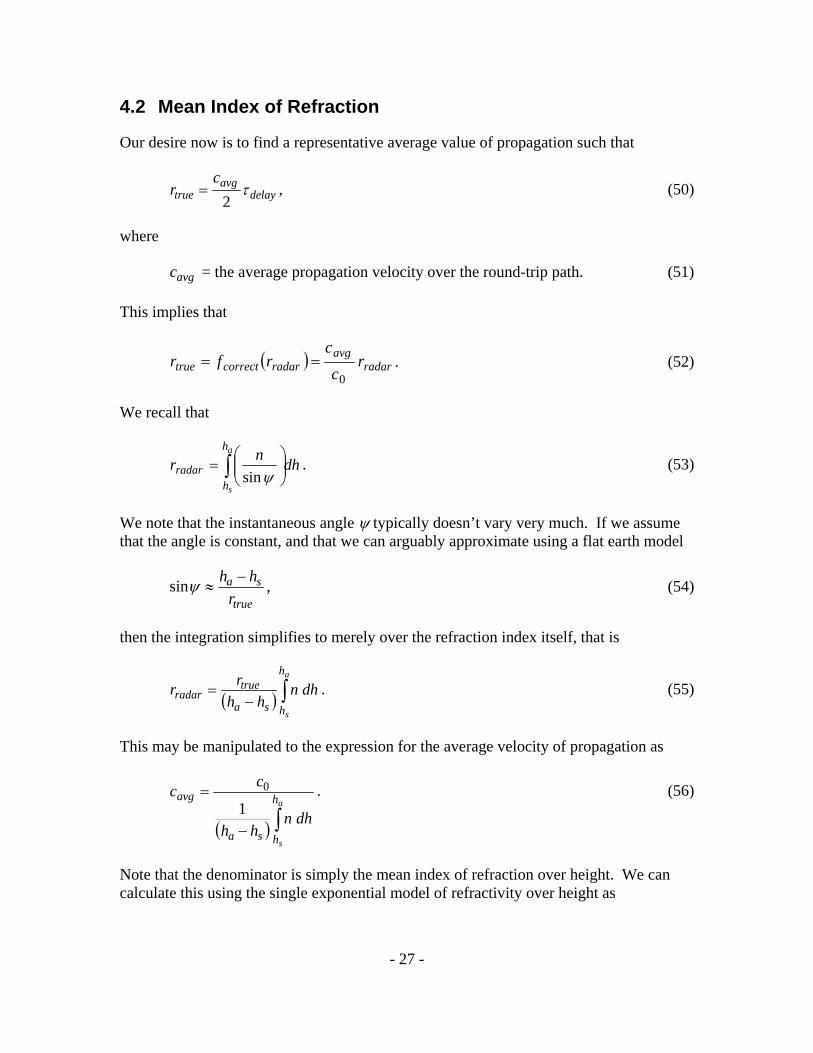
4.2 Mean Index of Refraction

Our desire now is to find a representative average value of propagation such that

delayavg

truec

r 2

, (50)

where

avgc = the average propagation velocity over the round-trip path. (51)

This implies that

radaravg

radarcorrecttrue rc

crfr

0

. (52)

We recall that

dhn

ra

s

h

hradar

sin. (53)

We note that the instantaneous angle typically doesn’t vary very much. If we assume that the angle is constant, and that we can arguably approximate using a flat earth model

true

sa

r

hh sin , (54)

then the integration simplifies to merely over the refraction index itself, that is

dhnhh

rr

a

s

h

hsa

trueradar

. (55)

This may be manipulated to the expression for the average velocity of propagation as

dhnhh

cc

a

s

h

hsa

avg

1

0 . (56)

Note that the denominator is simply the mean index of refraction over height. We can calculate this using the single exponential model of refractivity over height as

- 28 -

-0.05

-0.02

-0.02

-0.01

-0.01

0

0

0.01

0.01

0.02

0.02

0.05

0.05

0.05

0.1

0.1

0.1

0.2

0.2

0.2

0.5

0.5

1

1

2

2


rada

r he

ight

- k

ft


0 20 40 60 80 100 120 140 160 180 2000

10

20

30

40

50

60

(a)

-0.05 -0.02

-0.02

-0.01

-0.01

0

0

0.01

0.01

0.01

0.02

0.02

0.02

0.05

0.050.1

0.1

0.2

0.2

0.5

0.5

1

1

2


rada

r he

ight

- k

ft


0 20 40 60 80 100 120 140 160 180 2000

10

20

30

40

50

60

(b)

-0.2

-0.2

-0.2

-0.2

-0.1

-0.1

-0.1

-0.1

-0.1

-0.0

5

-0.05

-0.05

-0. 0

2

-0.02

-0.0

1

-0.01

0 0

0

0

0.01

0.01

0.02

0.02

0.05

0. 05

0. 1

0 .1

0. 2

0.2

0.5

0.5

1

1

2


rada

r he

ight

- k

ft


0 20 40 60 80 100 120 140 160 180 2000

10

20

30

40

50

60

(c)

Figure 11. True range estimation error of the mean index of refraction model compared to numerical integration of the segmented Bean and Thayer model. Target height for these plots is assumed to be 0.

- 29 -

dheNhh

dhnhhc

c a

s

b

sa

s

h

h

H

hh

ssa

h

hsaavg

60 101

11. (57)

Carrying out this integration yields the closed-form solution

b

sa

H

hh

sa

sb

avge

hh

NH

c

c1

101

60 . (58)

Rearranging this yields the following expression for average velocity of propagation as

b

sa

H

hh

sa

sb

avg

ehh

NH

cc

110

16

0 . (59)

This allows us to write the calculation for true range as

radarH

hh

sa

sbradarcorrecttrue re

hh

NHrfr b

sa1

6

110

1

. (60)

Note that since the denominator is so close to one, this may also be approximated as

radarH

hh

sa

sbradarcorrecttrue re

hh

NHrfr b

sa

110

16

. (61)

Figure 11 details the error of this model compared to the Bean and Thayer segmented model. We observe that even for worst case dry air, the error is less than 1 m out to 120 km ground range, and not much more than 2 m out to 200 km ground range, over the entire 0 to 65 kft altitude range.

- 30 -

Comparison to Robertshaw Model

It is interesting to compare this model to the Robertshaw empirical model. Although this mean index of refraction model is a little more complicated than the Robertshaw empirical model, it is more of an analytical approximation and does not fall apart at nearer ranges and lower altitudes.

This model, along with ‘truth’ points from the Robertshaw model, is shown in Figure 12. This model matches the truth points with an RMS error of 1.06 m.

Consequently, we observe that even over the data set that Robertshaw provided with his empirical model, the mean index of refraction model provides a somewhat better fit.

Interestingly, by making the refractivity versus height model more accurate at lower altitudes by selecting for the single exponential model the parameters

m 9144 kft 30 bh , and

9.102bN N-units, (62)

we can improve the match to Robertshaw’s truth points to an RMS error of 0.85 m.

An optimization of these parameters for Robertshaw’s truth points is beyond the scope of this report.

0 20 40 60 80 100 120 140 160 180 2000

10

20

30

40

50

60

range - km

rang

e er

ror

- m

15 kft - blue35 kft - magenta45 kft - green65 kft - red

Figure 12. Solid lines represent the mean index of refraction model, whereas asterisks represent ‘truth’ data from the Robertshaw model. Each color quartet represents Ns values of 250, 300, 350, and 400 N-units.

- 31 -

5 Range Correction Strategies

Once we have estimated the range correction applicable to our radar data, for example a SAR image, the question becomes “When do we actually apply the correction?” We examine two principal strategies below.

5.1 Real-Time Correction

Employing an average velocity of propagation calculated using for example the mean index of refraction lends itself to real-time correction of the raw radar data itself, as an integral part of timing and control equations.

Pros:

The prospect that the radar products emanating from the radar itself are already compensated for the atmosphere is very enticing.

Cons:

The velocity of propagation used for, say, different SAR images will itself likely be different for each image. Consequently, a SAR image’s pedigree (header or other auxiliary meta-data) really needs to contain the specific velocity of propagation employed during its real-time data collection and processing. This would be required to facilitate any post-processing to enhance range accuracy even further should newer or better environmental data be secured.

5.2 Post-Processing Correction

Employing a constant reference velocity of propagation (say, for free space) is the conventional technique for real-time processing. Any range accuracy improvement would need to be a post-processing correction.

Pros:

The advantage of this strategy is that the real-time data collection and processing are simple, conventional, and with predictable characteristics. Since free-space velocity of propagation is well-known, it need not be incorporated in the radar product’s header or meta-data. Any post processing does not have to ‘guess’ at what corrections might, or might not, have been employed during real-time processing.

Cons:

This strategy guarantees that real-time data products coming out of the radar have no compensation at all. These products would definitely require a post-processing stage to do any kind of range accuracy enhancement.

- 32 -

5.3 Which is Best Strategy?

To first order, there is no ‘best’ strategy.

However, there is one strategy that definitely is ‘worst’. This would be the case of using a non-standard reference velocity of propagation during real-time data collection and processing, however it might be calculated, and not reporting its value in the radar product’s (e.g. SAR image’s) header or meta-data. This tactic actually ‘adds’ uncertainty to the radar product instead of reducing it.

This author’s advice is “Don’t do this.”

- 33 -

6 Conclusions

We summarize herein the following.

Radar systems essentially make timing measurements between transmitted and received echo signals. Range is calculated with some assumption of the velocity of propagation of the radar waveform energy.

The atmosphere’s dielectric properties, principally owing to its temperature, humidity, and pressure, will affect the propagation velocity. Furthermore, the atmospheric properties vary with altitude, effecting refraction to yield non-straight-line propagation as well as non-uniform propagation velocity.

Actual propagation velocity deviations from the simplest free-space model impart an error in the calculated range. These errors can easily exceed 300 ppm in some circumstances.

Various models for atmospheric characteristics and their effects on radar signal propagation have been developed. These models can often be further simplified and approximated to yield corrections to range measurements. This has been done in this report.

- 34 -

“We find no sense in talking about something unless we specify how we measure it; a definition by the method of measuring a quantity is the one sure way of avoiding talking nonsense...” — Sir Hermann Bondi

- 35 -

Appendix A – Estimating Surface Refractivity

The principal cause of range error in the atmosphere is its refractivity function along the propagation path, mainly due to water content. Short of measuring this directly, which is decidedly impractical, we are limited to using reasonable models. We have in fact modeled this as a dependent principally on the surface refractivity, and referenced maps of mean values for these for the continental US. Of course, if we have better information of surface refractivity at the place and time of our radar data collection mission, rather than simple regional averages, then we may be able to improve our range error estimates. Towards this end, it is useful to be able to estimate surface refractivity based on more commonly available atmospheric metrics, such as temperature, relative humidity, and barometric pressure. We relate these here.

Smith and Weintraub6 present the following model for calculating refractivity

s

ss

ss T

ep

TN 4810

6.77, (A1)

where

sp = total atmospheric pressure in millibars (mb), or hectoPascals (hPa),

se = partial pressure of water vapor in millibars (mb), or hectoPascals (hPa),

sT = absolute temperature in Kelvin (K). (A2)

We have added the subscript “s” to these parameters to denote their being target surface parameters. We also note that

1 mb = 1 hPa. (A3)

Smith and Weintraub indicate that this model is accurate “to within 0.5% over a parameter space limited to temperature ranges of 50 to +40°C, total pressures of 200 to 1,100 mb, water vapor partial pressures of 0 to 30 mb and a frequency range of 0 to 30,000 mc [MHz]”.

We now examine these individual terms.

Absolute Temperature

Absolute temperature is pretty straightforward. We note that

0 C = 273.15 K, (A4)

with equal numerical increments.

- 36 -

Partial Pressure of Water Vapor

More commonly, this is expressed in terms of Relative Humidity. Accordingly, we identify the partial pressure of water vapor as

ssatss ee , , (A5)

where

s = surface relative humidity, with 10 s , and

ssate , = surface saturation water vapor pressure. (A6)

The saturation water vapor pressure has been modeled with several different equations, some quite elaborate. We will use an approximation known as the Antoine equation, namely

7240.39

63.17301962.8

, 10 sTssate mb. (A7)

This approximation is designed for the range 9915.2730 T .

Another approximation might be

787662.015.273030964.015.273000098.0,

2

10 ss TTssate mb. (A8)

This approximation is designed for the range 5015.2730 T . It matches the Antoine equation pretty closely over this range.

It is useful to note that the temperature at which the relative humidity is unity is the “dew point”.

Total Atmospheric Pressure

The total atmospheric pressure value that we need is that at the target surface, regardless of target surface’s altitude above sea level. However, when atmospheric pressure is reported by a station, it is customary to report the atmospheric pressure as some equivalent pressure at sea level. This equivalent Mean Sea Level Pressure (MSLP) is the atmospheric pressure normally given in weather reports in the media (radio, television, newspapers, internet, etc.).

We begin with an equation known as the Barometric formula, stated as

- 37 -

RL

gM

ss T

Lhpp

00 1 , (A9)

where

0p = sea-level reference atmospheric pressure in millibars (mb),

L = 0.0065 K/m = temperature lapse rate,

sh = target surface height above mean sea level in meters (m),

0T = sea-level reference atmospheric temperature in Kelvin (K),

g = 9.80665 m/s2 = gravitational acceleration at earth’s surface, M = 0.0289644 kg/mol = molar mass of dry air, R = 8.31447 J/(mol K) = universal gas constant. (A10)

In addition, the temperature at the target surface is modeled as

ss LhTT 0 . (A11)

These can be manipulated to the equation

RL

gM

ss

ss LhT

Tpp

0 . (A12)

This lets us use surface height, surface temperature, and sea-level pressure to calculate surface atmospheric pressure.

We note that we may calculate the exponent as

RL

gM 5.2558. (A13)

An average sea-level atmospheric pressure is commonly given as 1013.25 mb. Extreme atmospheric pressures (adjusted to sea level) might vary from 870 mb measured during Typhoon Tip in the western Pacific Ocean (1979) to 1092 mb measured in Tonsontsengel, Mongolia (2004). Extremes recorded for the United States range from 892 mb in Long Key, FL (1935), to 1064 mb in Miles City, MT (1983).

- 38 -

Putting it All Together

Given the following parameters

sh = target surface height above mean sea level in meters (m),

celsiussT , = surface temperature in Celsius (C),

s = surface relative humidity, with 10 s , and

0p = sea-level reference atmospheric pressure in millibars (mb), (A14)

we may calculate the surface refractivity with the following sequence of equations.

First we convert the surface temperature to absolute, in Kelvin, as

15.273, celsiusss TT = surface temperature in Kelvin (K). (A15)

Then we calculate the surface water partial pressure in millibars (mb) as

7240.39

63.17301962.8

10 sTsse = water partial pressure in millibars (mb). (A16)

Then we calculate the surface atmospheric pressure in millibars (mb) as

RL

gM

ss

ss LhT

Tpp

0 = total surface atmospheric pressure in millibars (mb).

(A17)

Finally, we calculate the surface refractivity in N-units as

s

ss

ss T

ep

TN 4810

6.77. (A18)

- 39 -

Exploring Some Numbers

An average value for Ns for the continental US is given by Bean7 as 313 N-units, whereas Altshuler8 reports that his data shows that “the average global surface refractivity is 324.8 N-units and that the standard deviation of [his] sample is 30.1 N-units.”

We now offer some specific examples.

Example 1.

Consider the example of a spring early morning on a high plateau, with

sh = 2438 m (8000 ft),

celsiussT , = 4.44 C (40 F),

= 1, and

0p = 1013.25 mb. (A19)

Note that the specified temperature is the dew point. Under these conditions, we calculate the surface refractivity as

sN = 252. (A20)

Example 2.

Consider the example of a warm humid day on the sea coast.

sh = 0 m (0 ft) = sea-level,

celsiussT , = 29.44 C (85 F),

= 0.85, and

0p = 1013.25 mb. (A21)

Under these conditions, we calculate the surface refractivity as

sN = 402. (A22)

- 40 -

Some Plots

As an exploration of the sensitivity of surface refractivity to some of these input parameters, we offer some plots of surface refractivity contours for two parameters at a time.

Figure 13 shows surface refractivity as a function of atmospheric pressures (adjusted to sea level) and relative humidity, at 23 C and at sea level. This plot shows a much stronger dependence on relative humidity than on the atmospheric pressure itself. Figure 14 shows the same function, but at a surface temperature of 4 C. Note that cooler air with the same relative humidity has a lower water partial pressure, and thus yields a lower surface refractivity. Nevertheless, there is still a somewhat greater dependence on relative humidity than on the atmospheric pressure itself.

Figure 15 shows surface refractivity as a function of atmospheric pressures (adjusted to sea level) and target surface height, at 23 C and 50% relative humidity. This plot shows a much stronger dependence on target surface height than on the atmospheric pressure itself. Figure 16 shows the same function, but at a surface temperature of 4 C. As with earlier plots, the cooler air with the same relative humidity has a lower water partial pressure, and thus yields a lower surface refractivity.

Figure 17 shows surface refractivity as a function of atmospheric pressures (adjusted to sea level) and target surface temperature, at sea level and 50% relative humidity. This plot shows a much stronger dependence on target surface temperature than on the atmospheric pressure itself, at least for the higher temperatures. Figure 18 shows the same function, but at a surface relative humidity of just 25%. The dryer air clearly offers a lower surface refractivity, and also reduces somewhat the surface refractivity sensitivity to temperature.

- 41 -

250

275

275

275

300

300

300

325

325

325

350

350

350

375

atmospheric pressure (mb)

rela

tive

hum

idity

Ts = 23 C, h

s = 0 kft

900 920 940 960 980 1000 1020 1040 10600

0.1

0.2

0.3

0.4

0.5

0.6

0.7

0.8

0.9

1

Figure 13. Surface refractivity as a function of surface relative humidity and MSLP.

275

275

300

300

300

325


rela

tive

hum

idity

Ts = 4 C, h

s = 0 kft

900 920 940 960 980 1000 1020 1040 10600

0.1

0.2

0.3

0.4

0.5

0.6

0.7

0.8

0.9

1

Figure 14. Surface refractivity as a function of surface relative humidity and MSLP.

- 42 -

250

250

275

275

275

300

300

325


heig

ht -

kft

Ts = 23 C, RH = 0.5

900 920 940 960 980 1000 1020 1040 10600

1

2

3

4

5

6

7

8

9

10

Figure 15. Surface refractivity as a function of surface height and MSLP.

200225

225

225

250

250

250

275

275

300


heig

ht -

kft

Ts = 4 C, RH = 0.5

900 920 940 960 980 1000 1020 1040 10600

1

2

3

4

5

6

7

8

9

10

Figure 16. Surface refractivity as a function of surface height and MSLP.

- 43 -

275

300

300

325

325

325

350

350

350

375

375

375

400

400

400

425425

425

450


tem

pera

ture

- C

hs = 0 kft, RH = 0.5

900 920 940 960 980 1000 1020 1040 10600

5

10

15

20

25

30

35

40

45

Figure 17. Surface refractivity as a function of surface temperature and MSLP.

275

275

300

300

300

325

325

350


tem

pera

ture

- C

hs = 0 kft, RH = 0.25

900 920 940 960 980 1000 1020 1040 10600

5

10

15

20

25

30

35

40

45

Figure 18. Surface refractivity as a function of surface temperature and MSLP.

- 44 -

“If it can't be expressed in figures, it is not science; it is opinion.” — Robert Heinlein

- 45 -

References

1 Harold D. Black, “An Easily Implemented Algorithm for the Tropospheric Range Correction”, Journal of Geophysical Research, Vol. 83, No. B4, April 10, 1978.

2 Andrew D. Goldfinger, “Refraction of Microwave Signals by Water Vapor”, Journal of Geophysical Research, Vol. 85, No. C9, September 20, 1980.

3 G. A. Robertshaw, “Range Corrections for Airborne Radar - A Joint STARS Study”, Project No. 6460, Report number MTR-9055, ESD-TR-84-169, The MITRE Corporation, May 1984.

4 Armin W. Doerry, “Earth Curvature and Atmospheric Refraction Effects on Radar Signal Propagation”, Sandia Report SAND2012-10690, January 2013.

5 B. R. Bean, G. D. Thayer, “Models of the Atmospheric Radio Refractive Index”, Proceedings of the I.R.E., Vol. 45, Issue 5, pp. 740-755, May 1959.

6 Earnest K. Smith, Jr., Stanley Weintraub, “The Constants in the Equation for Atmospheric Refractive Index at Radio Frequencies”, Proceedings of the I.R.E., Vol. 4, Issue 8, pp. 1035-1037, August 1953.

7 Bradford R. Bean, “The Radio Refractive Index of Air”, Proceedings of the I.R.E., Vol. 50, Issue 3, pp. 260-273, March 1962.

8 Edward E. Altshuler, “Tropospheric Range-Error Corrections for the Global Positioning System”, IEEE Transactions on Antennas and Propagation, Vol. 46, No 5, pp. 643-649, May 1998.

- 46 -

Distribution

Unlimited Release

1 MS 0532 J. J. Hudgens 5240

1 MS 0519 J. A. Ruffner 5349 1 MS 0519 A. W. Doerry 5349 1 MS 0519 L. Klein 5349

1 MS 0899 Technical Library 9536 (electronic copy)

;-)

radar range measurements in the...

Documents