radiant energy transfer measurements in air · ilnl##iim#llll~lillill~l ii097442 nasa cr-585...
TRANSCRIPT

NASA CONTRACTOR
REPORT
RADIANT ENERGY TRANSFER MEASUREMENTS IN AIR
by EL Hosbizaki, A, D, Wood, J. C. Andrews, md K. E(. lfG%o,n . .
Prepared by
LOCKHEED AIRCRAFT CORPORATION
Palo Alto, Calif.
for Western Operations Office
NATIONAL AERONAUTICS AND SPACE ADMINISTRATION . WASHINGTON, D. C. .’ SEPTEMBER 1966
- 4
https://ntrs.nasa.gov/search.jsp?R=19660027015 2020-05-06T13:03:24+00:00Z

TECH LIBRARY KAFB, NM
Ilnl##IIM#llll~lIllIll~l
II097442 NASA CR-585
RADIANT ENERGY TRANSFER MEASUREMENTS IN AIR
By H. Hoshizaki, A. D. Wood, J. C. Andrews, and K. H. Wilson
Distribution of this report is provided in the interest of information exchange. Responsibility for the contents resides in the author or organization that prepared it.
Prepared under Contract No. NAS 7-359 by LOCKHEED AIRCRAFT CORPORATION
Palo Alto, Calif.
for Western Operations Office
NATIONAL AERONAUTICS AND SPACE ADMINISTRATION
For sale by the Clearinghouse for Federal Scientific and Technical Information Springfield, Virginia 22151 - Price $3.00


FOREWORD
The work described in this report was completed for the
National Aeronautics and Space Administration Headquarters,
under the terms and specifications of their Contract NAS 7-359,
issued through their Western Operations Office, 150 Pica
Boulevard, Santa Monica, California - 90406.
This work was performed .in the Lockheed Missiles & Space
Company Aerospace Sciences Laboratory under R. D. Moffat,
Manager.
. . . 111

.-- _ . .-_._ . . . .

CONTENTS
Section
5
FOREWORD
ILLUSTRATIONS
NOTATION
INTRODUCTION
DISCUSSION OF THE PROBLEM
ANALYSIS
3. 1 Continuum Radiation
3.2 Line Radiation
3.3 Gage Surface Absorptance
3.4 Effect of Cavity Plume
3.5 Orfice Outflow Effect
3. 6 Radiation Cooling and Non-Equilibrium Radiation
EXPERIMENTAL METHOD
4.1
4.2
4.3
4.4
4.5
4.6
4.7
4.8
4.9
Shock Tube
Gage-in-Cavity Model
Thin-Film Gage Construction
Gage Box Circuit Analysis
Data Reduction
Gage Calibration - Heat Lamp
Gage Calibration - Bridge
Comparison of Gage Calibration Results
Gage Time Response Check
4.10 Noise Problems
DISCUSSION OF RESULTS
Page
. . . 111
vii
ix 1
3
7
7
9
27
31
34
35
37
37
40
45
47
50
53
55
60
65
68
80
V

Section
6 CONCLUSIONS
Appendix
A CONTINUUM ABSORPTION COEFFICIENTS OF NITROGEN AND OXYGEN
B STREAM TUBE CHEMISTRY CALCULATION
REFERENCES
Page
88
89
97
100
vi
ILLUSTRATIONS
Page
Windowless Gage-in-Cavity Model 4 Flow Details in Cavity During Radiation Data Acquisition 5
Comparison of Biberman and Armstrong Continuum Absorption Coefficients for Air 10 Comparison of Biberman and Armstrong Continuum Absorption Coefficients for Nitrogen 11
Integrated Continuum Intensity 12 Monochromatic Continuum Intensity: T = 14,700”K; p/p, = 3.45 x 10⁻² 13 Monochromatic Continuum Intensity: ‘I’ = 17, OOCP K; p/p, = 3.18 x 1O-2 14 Effective Width of a Lorentz Line as a Function of Optical Depth 22 Monochromatic Intensity From an Isothermal Air Plasma: (a) T = 14,70O”K, p/p0 = 3.45 x 10⁻², I = 3 cm; (b) T = 14,70O”K, p/p0 = 3.45 X 10B2, 1 = 12 cm 23 Line Intensity From an Isothermal Nitrogen Plasma: (a) All Lines; (b) Lines Transmitted Through a Window and Window Plus Filter 26 Silicon Monoxide Coated Gage Surface Absorptance 28 Effect of Surface Absorptance and Window and Window Plus Filter Transmittance on Continuum Intensity: T = 14,700” K; P/PO = 3.45 x 10⁻² 29
Effect of Surface Absorptance and Window Transmittance on Continuum Intensity: T = 17,000“ K; p/p, = 3.18 X 10m2 30
Transmittance of Quartz (Suprasil) Window and Window Plus Wratten No. 25 Filter 32
Plume Flow Properties 33
The 12-m Arc-Driven Shock Tube at the Lockheed Palo Alto Research Laboratory 38
Examples of Shock Speed Measurement and Outputs of Profile Phototubes 41
Gage-in-Cavity Model 42
Figure
1
2
3
4
5
6
7
8
9
10
11
12
13
14
15
16
17
18
vii

Figure Page
19
20
21
22
23
24
25
26
27
28
29
30
31
32
33
34
35
36
37
38
39
40
41
Gage Field of View
Basic Thin Film Gage Element
Schematic of Gage Box Circuit
Heat Lamp Calibration Apparatus and Typical Output Traces
Computer Output for Gage No. 282
Bridge Calibration Circuit
Example of Bridge Calibration Including Actual Oscilloscope Trace and Data Reduction
Comparison of Results of Lamp and Bridge Calibration
Xenon Flash Results for Bare Gage
Xenon Flash Results for Gage With 4 min. of Silicon Monoxide
Correlation of Noise Traces With Incident Shock Position
Noise Traces After Addition of Ring
Examples of Traces Obtained Behind Suprasil Window
Examples of Traces Obtained Without Window
Schematic of Plasma Insulation Check Apparatus
Examples of Traces From Acceptable Gages in the Windowless Model
Examples of Traces From Rejected Gages in the Windowless Model
Radiant Intensity Data Obtained Behind a Quartz Window: T = 14,700”K; p/p0 = 3.45 x 1O-2
Radiant Intensity Obtained Behind a Quartz Window and Filter: T = 14,700” K; p/p, = 3.45 X 1O-2
Radiant Intensity Obtained Without a Window: T = 14,700” K; P/P, = 3.45 x 10⁻²
Radiant Intensity Data Obtained Behind a Quartz Window: T = 17,000”K;p/po = 3.18 X 1O-2
Radiant Intensity Data Obtained Without a Window: T = 17,000” K; P/P, = 3.18 x 10⁻²
Quantum Mechanical Correction Factor 5 (hv) Versus Frequency
44
45
48
54
56
57
61
62
66
67
69
71
72
73
75
77
78
81
83
84
86
87
96
. . . Vlll
NOTATION
A
A P
A*
C
C 0
cP
‘Pi
E
Eb
e
e 0
GDi
61 i
fi
E
h
m
I
IL
area of active element of thin film gage
area of aperture
area ratio (Sec. 4.8)
Planckian intensity (spectral), W/cm2-sr set -1
velocity of light in vacua, 3. 00 x 10 10 cm/set
constant in spectral absorption coefficient equation, cgs units
specific heat of gage substrate
ith species specific heat at constant pressure
total (AC + DC) voltage
constant voltage
time-varying component of E
differential output voltage of bridge
ith species dissociation energy
ith species ionization energy
.th oscillator strength of 1 bound-bound transition, dimensionless
total enthalpy
Planck constant, 6.62 x lO-27 erg set
local streamline static enthalpy
radiant intensity, W/cm’-sr or current through gage
current in reference leg of bridge
ix

IO ‘I1
Iv
K
k
k’
1
m
Ni
n
m. 1
P
P(x)
%
q
s
s*
R
R P
R1 R*
S. 1
T(x)
T
Bessel functions, Eq. (3.11)
spectral radiant intensity
gage calibration constant Eq. (4. ‘7)
Boltzmann constant, 1.38 x lo-l6 erg/k or thermal conductivity
grouping of gage properties Eq. (4.3)
total path length for intensity determination, cm
index used in Sec. 4.5
.th number density of 1 particles/cm3
species in continuum absorption coefficient equation,
running index (Sec. 4.5)
Molar fraction of i th species
power dissipation in gage
local streamline static pressure
radiative flux, W/cm2
heat flux absorbed by gage
constant value of a step function heat flux
reduced heat flux, q* = q/K
resistance of gage
resistor in bridge or gage box circuit used to approximate a constant current source
resistors in bridge (Fig. 24)
resistance ratio (Sec. 4.8)
integrated line strength
local streamline kinetic temperature
absolute temperature (“K) or surface temperature excess (Sec. 4)
X

t
U
ax)
wi
lb i
Y
Z. 1
CY
o! V
ii
P
ri
yi
8
A
time or dummy optical length variable
dimensionless frequency variable, hv/kT
local streamline fluid velocity
effective emission width of an isolated spectral line, set -1
rate of production of i th component (species)
coordinate in planar radiative transfer equation
charge on residual ion resulting from photoionization process
temperature coefficient of resistivity
spectral absorptance of gage surface
weighted gage absorptance, Eq. (4.12)
bridge constant, Eq. (4. 16)
term structure constant
half half-width of electron impact broadened line, set -1
angular variable in planar radiative transfer equation or angle between gage- aperture line and aperture normal
dummy time variable
continuum spectral absorption coefficient, cm -1
discrete spectral absorption coefficient, cm -1
spectral absorption coefficient including induced emission, cm -1
spectral frequency
frequency of line center for bound-bound transitions
quantum defect correction factor
density, gm/cm3 or distance between gage and aperture
xi

density of air at standard temperature and pressure, 1.29 x 10 -3 PO
gm/cm3 .
1’ , x1 partition function of the parent and residual atom of i th 0
species involved in 1 photoionization
7
+i
optical length variable
summed photoionization cross section for all low lying states of a complex atom, cm2
w solid angle subtended by aperture at gage
Subscripts
a& refer to the two part gage (Sec. 4.8)
i refers to ith bound-bound transition or refers to i th chemical species
G refers to gage under ambient conditions
V refers to frequency variable
Superscripts
C refers to continuum absorption process
L refers to discrete absorption process
xii

Section 1
INTRODUCTION
The transfer of radiant energy plays a fundamental role in the physical phenomena
associated with entry into planetary atmospheres at superorbital flight velocities. It
determines not only the radiative heat transfer but can also have an important effect
on the convective heating. The convective heating is affected ,by radiant energy trans-
fer through the radiation cooling effect and by the transfer of radiant energy between
the inviscid and viscous flow regions in the shock layer. At entry velocities between
two to three times satellite velocities, radiative heating and the proper evaluation of
the radiation-convective coupling effects become of primary importance. The under-
standing of the physical phenomenon of superorbital entry and our ability to correctly
predict the combined radiative and convective heating hinges on our knowledge of
radiant energy transfer.
Early theoretical work on the fundamental aspects of.radiant energy transfer in air
consisted primarily of calculations of integrated emission coefficients (Refs. 1 and 2)
which are related to the Planck mean absorption coefficient. These calculations of
the emission coefficient considered only the continuum free-free and free-bound
transitions over a limited frequency range. Discrete transitions (bound-bound) were
not included. The frequency range considered excluded the vacuum ultraviolet. Sub-
sequent theoretical work (Refs. 3, 4, and 5) has shown that free-bound transitions to
the ground state which produce photons with frequencies in the vacuum ultraviolet
can easily dominate the integrated emission coefficient. The magnitude of the absorp-
tion coefficients in this frequency range indicate that for most superorbital entry con-
ditions of interest, self-absorption cannot be neglected.
Experimental investigations have been carried out in shock tubes (Refs. 6 and 7) to
measure the integrated emission coefficient of air. These investigations employed
1

models in which a radiation gage was located behind a quartz window. The gage
measured the radiation from the shock layer gas. The quartz window serves as a
filter in that it absorbs the vacuum ultraviolet portion of the spectrum. The wave
lengths which are passed by the quartz window are sufficiently long to be unattenuated
by the shock layer gas. Thus the results of these experiments do not include the
vacuum ultraviolet nor the effect of self-absorption; two very important aspects of
superorbital entry radiation transfer.
The purpose of the present investigation is to obtain experimental data on the integrated
intensity of high temperature air, including the vacuum ultraviolet, under conditions
similar to those encountered during superorbital entry by full scale vehicles. The gas
path lengths considered varies between 1 and 12 cm. For these values of the gas path
length and the thermodynamic conditions considered, the effect of self-absorption is
very important. The experiments were carried out in a 12-in. I. D. arc-driven shock
tube. A gage-in-cavity model was used to measure the total intensity as a function of
gas path length. This model enables the total radiation from the gas in the reflected
shock region to be observed through a small windowless aperture. The radiation data
are recorded before the test gas arrives at the radiation gage. Thus the problem of
separating the radiative heating from the convective heating is avoided.

Section 2
DISCUSSION OF THE PROBLEM
The primary objective of this investigation was to obtain integrated intensity data
which includes the vacuum ultraviolet. This imposes the requirement that the radia-
tion detector observe the test gas sample without any intervening media which can
absorb or emit radiation in the vacuum ultraviolet. This requirement precludes the
use of windows. The basic idea employed to carry out these measurements is to
place a radiation detector in a cavity and measure the radiative flux through a small
windowless aperture before the test gas arrives at the detector sensing surface.
Figure 1 is a schematic of the gage-in-cavity model showing some of its details and
its location in the shock tube to enable the observation of the gas in the reflected shock
region. Four thin film heat transfer gages are located in each cavity, approximately
2 in. from a small windowless aperture. Optical stops are located on the floor which
allows selection of the gas path length. Flow details in the cavity during data acquisi-
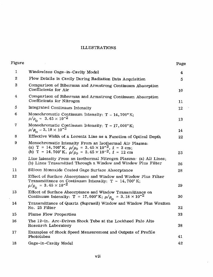
tion are shown schematically in Fig. 2. The purpose of the cavity is to allow the test
gas which flows through the aperture to expand quickly, thereby minimizing the absorp-
tion and emission from the expanding gas.
The chemical processes associated with the gas expansion in the cavity are not in
equilibrium. In order to properly assess the effect of the expanding gas on the data,
the number density and temperature distribution through the plume need to be deter-
mined. By making the assumption of radiative equilibrium, the absorption and emis-
sion by the plume can be evaluated using the number densities and kinetic temperature
obtained from the chemical non-equilibrium calculation. These calculations have been
carried out and are discussed in Sec. 3.
In addition to the effect of the plume, one must also consider the effect of test gas
outflow through the aperture. This outflow will create a small, time dependent,
3

1 DRIVER 1 /
RADIATION GAGE
TOP VIEW
SPLITTER PLATE
Y--l
Fig. 1 Windowless Gage-in-Cavity Model
4
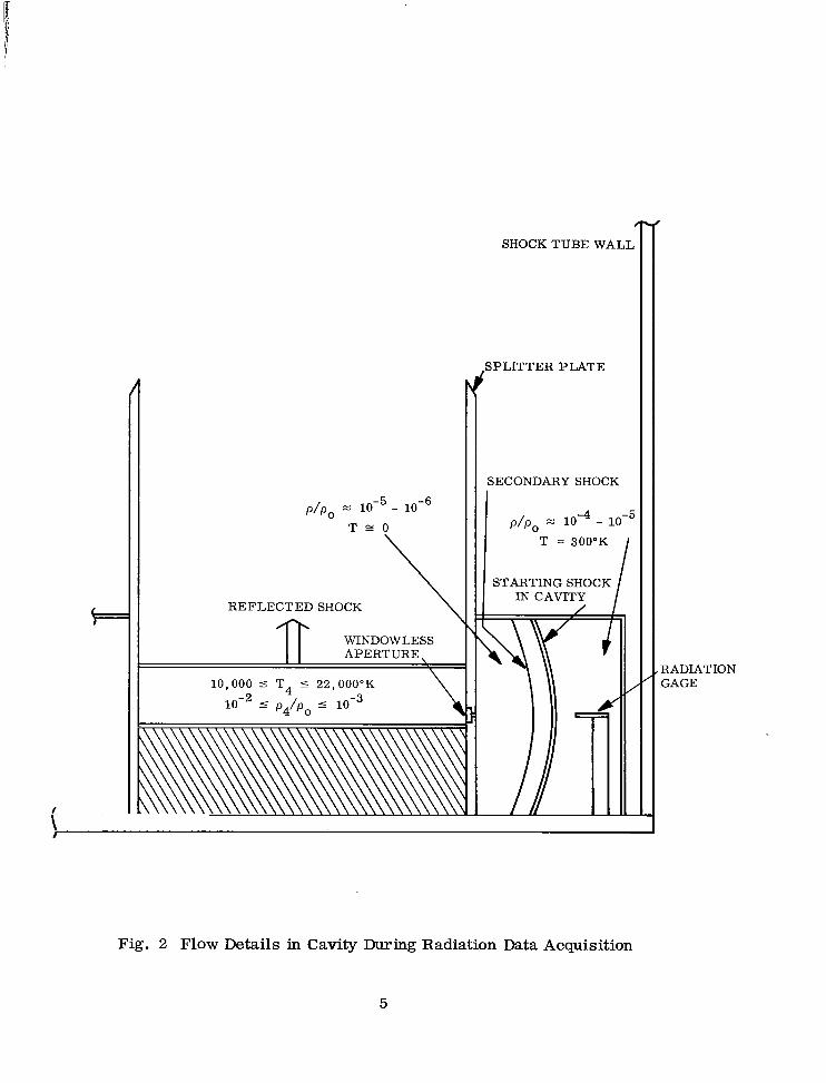
P/P, N 10-5 - 10-6
T=O
REFLECTED SHOCK
;:-
SHOCK TUBE WALL
SPLITTER PLATE
SECONDARY SHOCK
P/P, N 10-4 - 1o-5
T = 300°K
STARTING SHOCK IN CAVITY
RADIATION GAGE
Fig. 2 Flow Details in Cavity During Radiation Data Acquisition
5

non-uniform region near the aperture which could have a significant effect for short
testcgas path lengths. This possibility has also been investigated and is discussed in
Sec. 3. Other factors discussed in Sec. 3 are the possible effect of radiation cooling
on the thermodynamic state of the test case and possible non-equilibrium radiation
behind the reflected shock.
6

Section 3
ANALYSIS
3.1 CONTINUUM RADIATION
For a plane parallel slab of gas with temperature gradients in the normal direction
only, the expression for the net radiant flux is (Ref. 8)
000 s = 2n
II Ivy) 9 0) sin 8 cos 0 de dv (3.1)
0 0
where
a3 7 I/ I+T~, 0) =
I Bv(t, 4 e
-(t-7y) set 8 set 0 dt -
I Bv(t ,d e
-(TV-t) set 8 set 0 dt
7 0 V
Y
7 = V
I P”, dy
0
2hv3 Bv = - 1
C2 ehvlkT _ 1
The coordinate system employed is illustrated below.
Y
4 I,(e)
Ae
//I///
7

In the current experiment, 0 is restricted to small values so that we can set
set (e = 1 and assume that the monochromatic intensity IV is only a function of the
monochromatic optical depth 7y . The integration over the angle 8 can now be
carried out from which the intensity can be expressed as
g: I=o=
B (t v) e-(t-Tv) & - u ’
B (t v) e-(T”-t) dt dv v ’ 1 (3.3)
0
where the solid angle w is given by
8 w = 27r
I sin e de
0
Before the intensity can be evaluated for a particular situation, the absorption coeffi-
cient of the gas must be known as a function of the thermodynamic properties. The
temperatures which are of interest are sufficiently high that we can consider the gas
to be composed of nitrogen and oxygen atoms and ions only. The continuum abosorp-
tion coefficients (i. e. , photon absorption resulting from bound-free and free-free
transitions) are calculated from equations set down by Biberman (Ref. 9). Biberman’s
equations are based on an approximate treatment of the quantum defect method devel-
oped by Burgess and Seaton (Ref. 10) for calculation of the basic photon absorption
cross sections. This approximate theory is applicable to free-free transitions and
bound-free transitions from excited states for complex atoms such as nitrogen and
oxygen. The photon cross sections for bound-free transitions from the ground and
low-lying excited states are taken from Armstrong’s work (Ref. 3). Armstrong
has performed a very detailed cross section calculation using the quantum defect
method for photon frequencies lying near the threshold value and a high energy theory
for photon energies well above threshold. Armstrong’s calculations are felt to be
quite accurate and are used as a standard against which Biberman’s approximate

equations are compared. Such comparisons at typical plasma conditions of interest
are shown in Figs; 3 and 4. The particular equations used to calculate the continuum
absorption coefficient based on the methods summarized above are described in
Appendix A.
The intensity incident on the gage surface was calculated by means of Eq. (3.2) using
the absorption coefficient discussed above. The results are presented in Fig. 5 as a
function of, gas path length for several temperatures about the nominal experimental
values. The variation of intensity with temperature indicated by these results were
used to adjust the experimental data to a common temperature (17,000 and 14,7 OO’K
for the two experimental conditions considered). Also shown on Fig. 5 are the
intensity obtained by using Armstrong’s value of the absorption coefficient directly
rather than the curve fits. The agreement between the hand calculation and the com-
puter results using the analytical expressions for the absorption coefficient is very
good.
The monochromatic intensities for the two test conditions are shown in Figs. 6 and 7.
Note that for the present conditions, the vacuum ultraviolet is very close to the black-
body curve.
3.2 LINE RADIATION
The number of transitions between various atomic states in a plasma of complex atoms
and ions which give rise to discrete emission and absorption processes is typically on
the order of several hundred or more. Hence a systematic accounting of all these
transitions in a transport calculation appears impractical. Biberman (Ref. 11) and
Vorobev (Ref. 12) point out, however, ‘that only a relatively small number of transi-
tions, namely those involving the ground or low lying excited states need be considered
individually. The remaining transitions can be considered by aggregate formulas. We
have performed a somewhat more complete analysis of the line transport problem than
that reported by Biberman and his colleagues. In particular, we have considered

l-
I
I,
L
Fig. 3
ARMSTRONG
c-- BIBERMAN P = LOatm T = .14,00O”K
0 4 8 12 16 20 24 28 RADIATION FREQUENCY, hv (eV)
Comparison of Biberman and Armstrong Continuum Absorption Coefficients for Air
10

10-l v BIBERMAN
T = 16,OOO’K
P/P, = 10-2
1O-2 0 4 8 12 16 20 24 28
RADIATION FREQUENCY, hv (eV)
Fig. 4 Comparison of Biberman and Armstrong Continuum Absorption Coefficients for Nitrogen
11

,
0 HAND CALCULATION USING ARMSTRONG K
I I 1 I I I
2 4 6 8 10 12
OPTICAL PATH LENGTH, d (cm)
Fig. 5 Integrated Continuum Lntensity
12

BLACKBODY
I I 1 I I 4 8 12 16 20
RADIATION FREQUENCY, hv (eV)
Fig. 6 Monochromatic Continuum Intensity: T = 14,700”K; p/p, = 3.45 x 10m2
13

\
BLACKBODY
I I I _I I 4 8 12 16 20
RADIATION FREQUENCY, hv (eV)
Fig. 7 Monochromatic Continuum Intensity: T = 17,OOO”K; p/p0 = 3.18 x 10m2
14

more transitions* and used the oscillator strengths and half-widths for each individual
transition as calculated in detail by Armstrong (Ref. 3). For example, while Biberman
considers only transitions involving the lowest energy configuration of the parent core
electrons, Armstrong’s tabulation includes a large number of excited core parentages.
While certainly not dominant, these excited core transitions are not entirely negligible
and we have included those judged’ significant. On the whole, however, we have main-
tamed the spirit of Biberman’s approach by retaining only those transitions which
contribute significantly to the overall line transport.
The overall line transport problem can be examined in terms of the transport by a
single isolated line (or isolated groups of lines where overlapping is important). For
an isothermal plasma the total energy intensity including both continuum and discrete
processes, emergent in a given direction from a path length I , is
(3.3)
where /J’(V) is the continuum contribution to the absorption coefficient and ; P:(Y)
the sum of all discrete contributions to the absorption coefficient.
Equation (3.3) may be rewritten as,
I = [ B(V){ 1 - exp [+‘(u)I]] dv + 7 B(v) exp (-~:1) (1 - exp [- x/.$!(v)l]) dv
0 0 i
(3.4)
*The word transition is used in this report to define a multiplet array. The oscillator strengths and half-widths calculated by Armstrong are for the totality of individual line transitions within a given multiplet.
15

The first term on the right-hand side of Eq. (3.4) is simply the continuum portion of
the total intensity,
lcont. = [ B(v) {I. - exp [ -A~)Q]] dv 0
(3.5)
If the discrete contribution consists of a series of isolated lines (or groups of isolated
lines) for which $ (v) is finite only over a small interval Au. 1' then the secondterm
on the right-hand side of Eq. (3.4) becomes
I line = 1 exp (-b+) 1: i
(3.6a)
where
I: = Bi 1 { 1 - exp [-,L(v)l]] dv
AUi
(3.6b)
In Eq. (3.6) we have assumed that /J: and Bi are constant over each line interval
Avi . Combining Eqs. (3.5) and (3. 6) with Eq. (3.3) yields
I total = I cont. + 1 exp (-py Q) 1; (3.7)
i
Hence we can calculate the total intensity by separately calculating the continuum con-
tribution and each isolated line contribution and combining the contributions according
to Eq. (3.7). The basic problem in determining the energy transported by line emission
16

and absorption processes is thus the evaluation of 1: from Eq. (3.6b). Consider an
isolated line for which we represent the line absorption coefficient as
P;(P) = Sibi
where Si is the integrated absorptivity
co
I
2 si = p;(v) dv = +!& Nnfnn,
0
(3.3)
(3.9)
and hi(v) is the normalized line shape defined such that
I bi(“) dv = 1
The solution to the problem of line transport rests upon a knowledge of the oscillator
strength fnn, and line shape hi(v) .
Armstrong and his colleagues have calculated values of the oscillator strength for a
large number of multiplet transitions (including all significant transitions) in nitrogen
and oxygen atoms. It should be emphasized that Armstrong’s work represents the
culmination of a large research effort directed towards a precise theoretical deter-
mination of oscillator strengths using the best current quantum mechanical calcula-
tional methods. The soundness of Armstrong’s calculations can be judged by
comparison with recently published experimental data. Both the experimental data
obtained by Lawrence and Savage (Ref. 14), and the NBS tabulation (Ref. 15) of the
“best” experimental and theoretical values of atomic transition probabilities agree
well with Armstrong’s work, In particular, for the important “resonance” transitions
in the UV from the low-lying excited states to the ground states of nitrogen, Armstrong’s
f-numbers all agree within 25% of the measured values. The f-number calculation for
17

these “resonance” transitions are the most difficult and uncertain from a theoretical
viewpoint. Hence agreement with experiment for these transitions gives confidence
to the theoretical method.
It is of interest to compare Armstrong’s results with those of Vorobev (Ref. 12) and
Griem (Ref. 16). For both the transitions which lie in the W and in the visible+
regions of the spectrum, the Armstrong and Vorobev values for, the f-numbers agree
well; for most lines within 25% or less. Also, Griem’s values for the f-numbers for
transitions which lie in the visible+ region of the spectral agree quite well with those
calculated by Armstrong . However, for the important W transitions, Griem’s values
for the f-numbers are considerably lower than those calculated by Armstrong (and
Biberman) being lower by, typically, a factor of 30. This large discrepancy is due to
Griem’s use of Coulomb wave functions in evaluating the f-numbers for the transitions
to the ground states. Finally, it is important to note, that Griem’s tabulation of transi-
tions in the UV is not (nor was it intended to be) a complete list of the significance
transitions. Indeed, the nd - 2p, (n 5 4)) transitions which are not listed in Griem,
carry as much as 40% of the total radiative energy transported in lines at conditions
which are of interest from both experimental and reentry investigations, (see Ref. 12).
Hence the use of Griem’s f-number data in calculating radiative line transport willlead
to a large underprediction.
Griem (Ref. 16) has made detailed line shape calculations for isolated lines of low
atomic number elements including nitrogen and oxygen. Griem’s calculations lead to
the conclusion that,’ for the relatively dense plasmas of interest where the electron
number density is at least as large as 10 16 particles/cm3, electron impact broadening
dominates. The contribution from ion broadening under the quasi-static approximation
is on the order of a few percent and can be neglected for the purposes of transport
calculations. Hence, the lines acquire a Lorentz (dispersion) shape,
hi(v) = Yi’x
(v - v. 1
- di)2 + 7; (3.10)
18

with a (half) half-width yi and a line shift di . Griem’s calculations show that the
1ineC shift is of the same order as the half-width. Since the magnitude of the line shift
is not sufficiently great to produce overlapping on a multiplet basis, then for the iso-
thermal conditions of immediate interest, we can neglect the line shift term, di , in
Eq. (3.10). Then hi(v) is given by the somewhat more simple expression,
hi(v) = Yj,/’
(v - Vi)2 + y; (3.11)
In terms of Eq. (3. 11) the line shape is determined by the half-width yi . We have used
the half-widths calculated by Armstrong (Ref. 3) whose method follows the work of
Stewart and Pyatt (Ref. 17). A comparison of Armstrong’s half-widths with those pre-
sented by Griem shows Armstrong’s values to be consistently large by, roughly, a
factor of 5, in the temperature range of interest. Griem’s work is the most detailed
treatment currently available. As Griem points out, only the wave functions for the
upper state are required in the half-width calculation. Then the use of Coulomb wave
functions half-widths to calculate should be applicable without a serious degradation of
accuracy. Hence, the half-widths tabulated by Griem for transitions will be reasonably
accurate. Unfortunately, Griem tabulates half-widths for only three significant transi-
tions in the UV and a limited number for the visible-IR transitions. The only complete
tabulation of half-widths are those provided by Armstrong, which, from necessity, are
used in our analysis. The use of Armstrong’s y i values represents the largest source
of uncertainty in the theoretical line transport predictions,
Proceeding with the solution to the transport equation, we evaluated Eq. (3.6b) using
the line shape given by Eq. (3.11). Following the analysis of Plass (Ref. 18) for the
case of an isolated line with a Lorentz shape, the effective (emission) width of the th i
line is defined by
19

wi =B= ‘:: j- [l - exp[-$(v),])dv
AVi
and inserting the Lorentz shape in Eq. (3.12) yields
(3.12)
(3.13)
where 7i is the optical depth, py (u = vi )1 based on the absorption coefficient at the
line center, v = v. 1'
5 p+=ly = - =‘y* 1
and J o, J 1 are Bessel functions of an imaginary argument. The exact solution for the
effective width afforded by Eq. (3.13) is cumbersome as it involves the use of Bessel
functions. However, two useful limiting expressions for Wi are available. One is
the thin limit 7i << 1 , for which \ \
wi Ti -=- 27ryi 2 (3.14a)
and the other is the thick limit 7i >> 1 , for which
wi T l/2
i -= - 271Yi 0 7T (3.14b)
The “square-root” law of Eq. (3.14b) can be substantiated physically by realizing that
Eq. (3.14b) follows directly from Eq. (3.12) if we neglect the term 7: in comparison
20

to (V - yi)2 in the denominator in Eq. (3.11). Deleting -yF causes the absorption
coefficient to become infinitely large at the line center. However, if the actual
absorption coefficient is sufficiently large at the center, i. e., 7i >> 1 , then the
emission is already blackbody limited and no substantial error is encountered in
neglecting the 7: term. A comparison of the limiting solutions from Eqs. (3.14a)
and (3.14b) with the exact solution from Eq. (3.13) is shown in Fig. 8. The line
transport is evaluated from either Eq. (3.14a) for 7i < 1 or Eq. (3.14b) for ‘ri > 1 .
Reference to Fig. 8 shows that the maximum error of about 25% introduced by these
approximate relations is roughly at Ti = 1 . Since most of the transitions are at
conditions where 7i << 1 or 7. >> 1 , 1
the aggregate error is much less than the
maximum of 25%.
Calculations were made of the radiative intensity resulting from line transitions from
an isothermal nitrogen plasma. The following thermodynamic conditions were con-
sidered corresponding to the nominal experimental target conditions:
T= 14,700” K T = 17,OOO”K
P/P, = 3.45 x 1o-2 P/P, = 3.18 x 10 -2
where p, is the density at standard conditions, p 0 = 1.29 x 10s3 g/cm3.
The spectral distribution of the total intensity (continuum plus lines) is shown in
Figs. 9a and 9b for the 14,700” K temperature condition at pathlengths of 3 and 12 cm.
The monochromatic continuum intensity is taken from Fig. 6. The line intensity cal-
culated for each group of transitions is the total energy (i. e., spectrally integrated)
within that spectral group. To display the spectral location of the energy emitted in
lines, it is convenient to plot the equivalent width of blackbody intensity for each
group of lines. Thus the shaded areas limited by the blackbody intensity shown in
Figs. 9a and 9b represent schematically the line intensity. Each shaded area is
equal to the total line radiation from the transitions located within the isolated spectral
intervals shown. The numbers listed adjacent to each spectral group give the percent
21

I I I I I I I I 1
THIN
/’
/
/
/’
/
THICKAPPROXIMATION
A EXACTSOLUTION
2’ 0.1 0.2 0.4 0.6 0.8 1.0 2.0 4.0 6.0 8.0 10
OPTICALDEPTHAT LINE CENTER+
Fig. 8 Effective Width of a Lorentz Line as a Function of Optical Depth

1 N \-
II II I I I I T = 14.700’K
I
P/P, = 3.45 x 10-z
P =3cm
\ NOTE: NITROGEN LINES ONLY
WINDoW CUT-OFF-
CONTINUUM INTENSITY = 43% TOTAL
-1
P/P, =, 3.45 x 10⁻³
I
I
1 = 12cm
\ I’
NOTE: NITROGEN LINES ONLY
COMTTINUUM INTENSITY = 50% TOTAL
FREQUENCY, hv(eV) FREQUENCY, bu (eV)
WAVELENGTH, i(A) WAVELENGTH, $1
Fig. 9 Monochromatic Intensity From an Isothermal Air Plasma: (a) T = 14,70O”K, p/p0 = 3.45 x 10⁻², 1 = 3 cm; (b) T = 14,70O”K, p/p, = 3.45 X 10e2, I = 12 cm

of the total (continuum plus line) energy carried by each group of lines. For the case
where the lines within a spectral group are black and overlap (as occurs for most of
the important transitions at these dense plasma conditions), then the shaded areas in
Figs. 9a and 9b reflect the actual monochromatic intensity resulting from line
transitions.
Note the predominance of the W transitions in the line transport. We list below
some of the important transitions within the various spectral groups (see Moore’s
tables of energy levels (Ref. 19) for the spectroscopic notation):
Spectral Group
hv = 7.11 eV
hv = 8.30 eV
hv = 9.4 eV
hv = 10.4 eV
Multiplets
2p3 2p” - 3S2P
2P 3 2Do - 3S2P
2P 3 2$ - 3d 2D
2P 3 2po - 3d 2p
2P 3 4SO - 3s4p
2P 3 2Do - 4s
2P 3 2po - nd (nr4)
2P 3 2Do - 3d 2F
Except for the upper members of the 2p 32 o P - nd series, the above transitions are
low lying with relatively small half-widths. As a result, these lines are strongly
reabsorbed so that a knowledge of the line shape, particularly in the wings, is impor-
tant. Additionally, in the important spectral region from 10.0 eV to 10.8 eV, the
above lines overlap in terms of the effective emission widths. This overlapping must
be considered in order to calculate meaningful intensity values.
In the infrared portion of the spectrum, lines are relatively unimportant (in terms of
the total line transport) at short pathlengths but increase in importance at longer
24

pathlengths as will be observed by comparing Figs. 9a and 9b. In the infrared, the
important transitions are, primarily, the various multiplets in the 3s - 3p and
3p - 3d series.
The integrated line intensity is obtained by summing the contributions from the
spectral groups shown in Figs. 9a and 9b with the continuum attenuation included.
The resultant total line intensity versus pathlength prediction is the solid curves in
Fig. 10a. The region of transmittance of a Suprasil window and a Wratten bandpass
filter is shown in Figs. 9a and 9b. By summing only contributions which lie in these
spectral regions, the prediction of the line intensity transmitted by a window and
filter given in Fig. 10b is obtained.
A comparison of the line intensity predictions of Biberman, et. al (Ref. 20 ) at the
two thermodynamic conditions and at pathlengths.of 1 and 10 cm is included in
Fig. 10a. There are two sources of uncertainty in extracting an intensity value from
Biberman’s data. First, Biberman tabulates in Ref. 20 only the total (lines plus
continuum) flux emitted by an isothermal slab. An estimate is made of the relative
contribution of lines and continuum to the total flux based on graphs in Refs. 12 and
20. Finally, the line flux values thus obtained must be converted into an intensity by
estimating the effective solid angle for the energy transported in lines.
As mentioned above, Armstrong’s half-width values are larger than Griem’s values
by roughly a factor of five at the temperatures of interest for the transitions compared.
From a theoretical viewpoint, Griem’ s calculations are more accurate since Griem
has performed a more detailed solution. In order to assess the effect of uncertainty
in Armstrong’s half-width data, the line transport at T = 14,700” K was re-evaluated
using half-widths which were uniformly reduced by a factor of five from Armstrong’s
values. The resultant. line intensity is given by the dashed curve in Fig. 10a. It is
seen that the line intensity is reduced by about 30% uniformly with pathlength, con-
siderably less than the factor of five decrease in the half-widths. This relative
insensitivity of the total line intensity to changes in the half-width values is a result
25

lo4 r I I I I IPI
T = 17.000'K
WINDOW ONLY
WINDOW ONLY
--'wn?DOWPLUSFILTER PIP, = 3.45 x 10‘
/
/
(6)
102 I I I I I I 0 2 4 6 8 10 12
PATH LENGTH. f(cm)
I I I I I I
T = 17,OOO’K
P/P, = 3.18 x lo-:
3 I I I I I I ” 4 6 6 10 12
BIBERMAN'S DATA DENOTEDBY; l T = ll.OOO'K
A T = 14.700.K
PATH LENGTH !(cm)
Fig. 10 Line Intensity From an Isothermal Nitrogen Plasma: (a) All Lines; (b) Lines Transmitted Through a Window and Window Plus Filter

of three factors. First, the intensity from line transitions which are optically thin
is ‘independent of the half-width. Second, the intensity from line transitions which
are optically thick vary as l/2 y . Third, strong overlapping of optically thick lines
results in a y dependence which is much less than a one-half power variation.
3.3 GAGE SURFACE ABSORPTANCE
The radiative intensity measurements were carried out by means of platinum thin
film gages. The platinum films were coated with silicon monoxide or aluminum
black. The silicon monoxide provided an insulating surface over the platinum film
which was found necessary to prevent the gage from being shorted by the gas in the
cavity. The radiation from the test gas in the windowless configuration photo-
dissociates and/or photoionizes the gas in the cavity which causes the gages to short
to their surroundings if they are not insulated. At the lower of the two temperatures
investigated, nominally 14,700” K, the intensity incident upon the gages located behind
a quartz window were measured with platinum films coated with aluminum black. The
aluminum black has a very uniform (with frequency) absorptance close to unity.
Unfortunately, unlike aluminum black, the silicon monoxide coating does not absorb
uniformly over the radiation frequency range of interest. The surface absorptance
for several specimens, which were prepared in the same manner as the thin film
gages, were measured on a Beckman DK-2 spectrophotometer. The results of three
such measurements are presented in Fig. 11. These silicon monoxide absorptance
curves exhibit interference patterns in the near infrared. In the visible and ultra-
violet, the surface absorptance is more uniform and approaches unity at the higher
frequencies, (shorter wave lengths). Although these absorptance curves differ in
detail, when the monochromatic continuum intensity absorbed by the gage surface
is integrated over frequency, the variation in the integrated continuum intensity from
one absorptance curve to another is quite small as shown in Figs. 12 and 13. The
surface absorptance of the silicon monoxide coating reduces the radiative intensity
absorbed by the gage by 10 to 20% from the value assuming a surface absorptance
27

0. s
0. f
0.3
0.2
0.1
0
I-
I-
I -
ABSORPTANCE CURVE
NO. 1
----- NO. 2
---- NO. 3
I I I I I I I
0 1 2 3 4 5 6 7
RADIATION FREQUENCY, hv (eV)
Fig. 11 Silicon Monoxide Coated Gage Surface Absorptance
28

lo*
10
t-NO. 2 /
/ BLACK GAGES
WINDOW AND FILTER WITH ALUMINUM BLACK GAGES
0 2 4 6 8 10 12
GAS PATH LENGTH, 6 (cm)
Fig. 12 Effect of Surface Absorptance and Windown and Window Plus Filter Transmittance on Continuum Intensity: T = 14,700” K; P/P, = 3.45 x 10⁻²
29

I I I I I
SURFACE ABSORPTANCE = 1.0
SURFACE ABSORPTANCE CURVE (FIG. 11)
NO. 1
NO. 2
\ NO. 3\
Y /NO. 2 PLUS PLUME
NO. 2 WITH SUPRASIL wINDow
I I I I I -. 103 I 0 2 4 6 8
GAS PATH LENGTH, S (cm) 10 12
Fig. 13 Effect of Surface Absorptance and Window Transmittance on Continuum Intensity: T = 17,000” K; p/p, = 3.18 x lo-2
30

coefficient of unity. As the gas path length is increased, the infrared portion of the
spectrum becomes increasingly more important since it is not nearly absorbed as much
as the ultraviolet. This causes the silicon monoxide surface absorptance to have a
larger effect in reducing the intensity absorbed by the gage.
Also shown in Fig. 12 are the intensities incident upon the gage surface when a quartz
.window or a quartz window in combination with a filter is placed between the radiating
gas and the gage. Similar results are shown in Fig. 13 for the case of the quartz
window alone. The transmittance curves for the quartz window and the filter are pre-
sented in Fig. 14. These transmittance curves were obtained from measurements
carried out as part of the current investigation.
3.4 EFFECT OF CAVITY PLUME
When data without a window are being taken, the test gas expands into the cavity, form-
ing a time dependent plume which is at a lower temperature and density than the test
gas and hence is not expected to significantly absorb or emit radiation. However, to
verify this assumption, detailed calculations were carried out. The chemical pro-
cesses associated with this rapid expansion of the test gas are not in equilibrium. The
number density of the atoms and electrons and the kinetic temperature were calculated
using a one-dimensional, one-equilibrium streamtube analysis. This streamtube
analysis requires the pressure distribution along the streamline as input data. The
pressure distribution along the axial streamline was obtained from characteristic
solutions for steady state plumes in chemical equilibrium. The details of the stream-
tube analysis are presented in Appendix B.
In carrying out these non-equilibrium calculations it was assumed that the test gas
first expands to sonic conditions at the orifice. This expansion to sonic conditions
was assumed to be in chemical equilibrium. The non-equilibrium streamtube analysis
was then used to calculate the number densities and temperature along the axial stream-
line. The results of these calculations are presented in Fig. 15. These number
densities and temperature profiles were used to calculate the absorption coefficient
31

100
90
80
7c
s
3 6C
2 E 5(
52
3(
2(
11
/
,-
I-
I-
I-
)-
I-
)-
I-
or
o-
QUARTZ WINDOW \-bf
‘PLUS WRATTEN NO. 25 FILTEI
I I - 0.2 0.4 1.0 2
RADIATION FREQUENCY, hv (eV)
4 6 8 10
Fig. 14 Transmittance of Quartz (Suprasil) Window and Window Plus Wratten No. 25 Filter

(NJ
(T) * __----------- ----ma_
(0)
PLUME EXPANSION, NON-EQUILIBRIUM PARTICLE DENSITY INITIAL CONCENTRATIONS SET AT SONIC ORIFICE CONDITIONS \
RESERVOIR CONDITIONS (EQUILIBRIUM) T=17,000’K, P=Gatm SONIC ORIFICE CONDITIONS (EQUILIBRIUM) STARTING CONDITIONS AT x = 5 x 10e4 cm (EQUILIBRrUM)
T = 15,90O’K, P = 3.3 atm T = 15, SOO”K, P = 3.29 atm
I I
POSITION 1 OF GAGE 1
I I I I I I I
I I I I I I
I I
1015 ’ I I II I I I, I I III I I Ill I 1 I I I lo2
1o-4 10-3 1O-2 10-l 1 10
DISTANCE DOWNSTREAM FROM SONIC ORIFICE (cm)
Fig. 15 Plume Flow Properties

and the resultant intensity to the gage surface. These results are shown in Fig. 12,
where it is seen that the absorption by the plume is negligible. In these calculations
the intensity was evaluated along the plume axis so that the emission from the plume
itself was not included. The number density and temperature profiles normal to the
plume axis are not known and hence a precise evaluation of the emission from the
plume cannot be carried out. However, the temperature along the axis decreases
rather rapidly and it is expected that the temperature will decrease in a similar manner
along the neighboring streamlines. If this is the case, the emission from the plume will
be negligible since only a small fraction of the plume near the orifice will emit to any
significant degree. Furthermore, the maximum plume temperature is the temperature
of the gas at the orifice so that the emission per unit mass from the plume is signifi-
cantly less than that in the test gas.
3.5 ORIFICE OUTFLOW EFFECT
When the test gas expands into the cavity an expansion wave will be propagated into the
test gas. This expansion wave will lower both the number densities and the tem/pera-
ture in the region near the orifice. This non-uniform region near the orifice is, of
course, time dependent. It has been estimated that the expansion wave will travel
approximately 4 cm in 10 psec. The change in the number density and temperature
caused by the passage of the expansion wave has not been precisely evaluated. The
possible effect of this expansion wave in reducing the radiative intensity was investi-
gated experimentally by obtaining intensity data behind a window with the window placed
at the aperture and on subsequent shots, with the window moved back from the aperture
and placed in front of the gage. With the window at the aperture, there is no gas
expansion into the cavity. With the window placed immediately in front of the gage,
which is located approximately 5.6 cm from the aperture, the test gas will expand into
the cavity. The data obtained with the windows placed as -described above, show no
discernible differences. The intensity data obtained are discussed in Sec. 5. From
these results it was concluded that the expansion wave in the test gas has no measurable
effect on the intensity data.
34

3.6 RADIATION COOLING AND NON-EQUILIBRIUM RADIATION
In the current experiment, the temperature behind the incident and reflected shocks
are sufficiently high so that the possible effect of energy loss by radiation must be
considered. Radiation cooling can affect shock tube flows by two means. The first is
by attenuation of the incident shock caused by radiation cooling of the gas behind the
incident shock. The second is by cooling of the test gas behind the incident shock and
in the reflected shock region.
A simplified analysis of the effect of radiation cooling on the flow properties behind
the incident shock was carried out in Ref. (21). In this analysis, the gas was assumed
to be optically thin and simple approximate expressions were used for the integrated
emis sivity . The results indicate that for the shock velocities (9.5-10.5 mm/psec)
and initial pressures (0.200 Torr) of this experiment, radiation cooling will have a
negligible effect on the gas properties behind the incident shock. The analysis, how-
ever, neglects the vacuum ultraviolet and self-absorption. These two effects com-
pensate each other and the results of the analysis should be indicative of the actual
condition.
The effect of radiation cooling on the test gas in the reflected shock region is much
more difficult to assess. The reason being that neither the quantity of test gas in the
reflected shock region is precisely known nor is the emission from the driver gas.
The cooling of the test gas is dependent on the net exchange of radiant energy between
the test gas, the driver gas and the surrounding surfaces. An estimate of the energy
lost by radiation indicates that if one neglects the radiant energy transfer from the
driver gas, approximately 10% of the internal energy will be lost in 10 psec. This
decrease in internal energy will result in approximately a 10% decrease in temperature
and a 10 to 20% decrease in the radiant intensity. This slight decrease in the radiant
intensity is evident in some of the photomultiplier records which are used to monitor
the test gas (see Sec. 4.2). The resolution of the thin film heat transfer gages, how-
ever, is not sufficient to consistently detect this radiation cooling effect.
35

One of the fortunate circumstances of the present experimental setup is that the non-
equilibrium region will move out of the field of view of the radiation gages. Based on
the ionization rate data presented in Ref. 22, the time for the ionization relaxation
zone to move out of the field of view of the gages has been estimated to be between 2
and 4 psec. This time is comparable to the time necessary for the reflected shock to
move across the field of view of the gages and is an inherent initial transient in this
experiment. It appears, therefore, that non-equilibrium radiation is not an important
consideration.
36

Section 4
EXPERIMENTAL METHOD
4.1 SHOCK TUBE
The LMSC 12 in. arc-driven shock tube was used exclusively in this research. The shock tube driver had an inside diameter of 2-3/4 in. and was 30 in. long. The driver gas was helium at 100 psig initially and was heated by a 30-in. axially-concentric arc
struck between a beryllium-copper anode and a stainless steel diaphragm. The driver contained a Lexan liner with a l/8 in. thick wall and which lasted about 25 shots on the
average.
The energy for the arc was supplied by a 4800~PF capacitor bank capable of being
charged to 20 kV. The first of the two experimental shock tube conditions used in this
research was obtained by charging the full bank to 12 kV resulting in an available
energy of 350,000 J. This would drive the incident shock at about Mach 30
(10.5 mm/psec). The other and lower temperature condition was obtained by dis-
connecting 3/8 of the capacitor bank and holding all other parameters constant, Here
incident shock Mach numbers of about 25.4 (8.9 mm/,usec) were obtained. In both
cases the residual bank voltage of typically 4.5 kV meant that about 85% of the avail-
able energy was utilized.
The driver and driven sections were connected by a 4-ft shock formation section with
a 3-in. inside diameter followed by a conical transition section. This section expanded
the inside diameter from 3 to 12 in. and had a lo-deg half-angle with both the entrance
and exit regions contoured to minimize the effect of secondary shock waves.
The driven section was 38 ft long with a nominal inside diameter of 12 in. and is shown
in Fig. 16. The stainless steel driven section had a 32-pin. finish and the concentricity
37

Fig. 16 The 12-in. Arc-Driven Shock Tube at the Lockheed Palo Alto Research Laboratory

of the three 12 ft sections was held to f 0.002 in. to minimize disturbances at the
joints. The driven section was pumped through a large contour valve in a 2-ft section
located at the driver end of the tube.
The test gas was bottled air obtained from the Matheson Company and labeled 21% 02,
balance N2. This gas was purified by passing it first through a dry ice-acetone cold
trap, then through a 6-ft length of tubing filled with Ascarite to remove CO2 as a
possible impurity, and finally through 6 ft of Drierite (C&O,) to remove any residual
water vapor. All experiments were performed at an initial driven section pressure,
P1, within 1% of 200 p. The tube was filled through a sm.all storage reservoir and
the entire filling system was calibrated with a McLeod gage. Prior to each shot the
tube was evacuated to below 1 p and purged several times with test gas. The leak
rate was always below 1 &min and a time of 1 min was required between closing the
contour valve and firing the tube.
The shock tube was contaminated after each shot by a very fine black dust from the
Lexan liner. This was removed by pulling a dry rotating brush through the tube
followed by several passes with dry cloth wipers wrapped around the brush. Then
all joints and instrumentation parts were opened and wiped clean. On several occa-
sions the tube was thoroughly cleaned with soap and water but there was no noticeable
change in the radiation data after this more extensive cleaning.
All the shock tube instrumentation was located in the last 12 ft of the driven section.
This included a vacuum gage (NBC Equipment Corp. , Alphatron), the test gas
reservoir, an incident shock profile phototube, and three ionization-type shock speed
detectors. Most of these items are visible near the top of Fig. 16.
The shock speed detectors were spaced 1 ft apart and the last one was located slightly
behind the leading edge of the model splitter plates. The outputs of the shock speed
detectors were displayed on oscilloscopes using Textronix .type 53/54D plug-in units
operated in the A-B mode. .Thus the outputs of two adjacent detectors were displayed
39

on the same calibrated sweep trace as shown in the top of Fig. 17. It was estimated
that the time interval could be determined to f 0.5% and since the distance between the
detectors was much better known, the shock speed was measured to f 0.5%. The
difference between the two shock speed measurements obtained from the three detectors
was always within this uncertainty. The temperature and density of the test gas behind
the reflected shock were obtained from the recent report by Laird and Heron (Ref. 23).
The quality of each shot was assessed from the output of a collimated phototube
located about 4 ft upstream of the model and which measured the radiation profile
along the incident shock. Examples of this profile are given on Fig. 17 for the two
test conditions used in this research. Here the incident shock and the interface
arrival are clearly seen. The non-equilibrium radiation overshoot was clearly visible
at MS = 25.4 conditions but was not apparent at MS = 30.1. The precursor radia-
tion apparent on these traces is attributed to scattering off the opposite wall of the
shock tube. The quality of the shot was a much stronger function of the diaphragm
parameters (thickness and depth of scribe) than had heretofore been suspected. Opti-
mum values were stainless steel 0. 093-in. thick and scribed 0.053-in. deep.
4.2 GAGE-IN-CAVITY MODEL
The gage-in-cavity model is best described from the three views shown in Fig. 18.
The photograph at the lower left shows the model ready for insertion into the end of
the shock tube with the exception of a top ring which is discussed in Sec. 4.10. The
view at the upper-left shows the model rotated 90 deg and with a cavity cover removed.
Here four thin film gages with taped and magnetically shielded leads are visible. These
gages were pointed toward the windowless aperture which is also visible immediately
above the gages. The object between the gages is a Pyrex light pipe which was colli-
mated to give the same field of view as the gages. The light was fed to a cavity
profile phototube through a flexible fiber optic bundle. The output of this phototube
was used to provide a time reference and also to determine the time variation of the
radiation (at least the visible part of it) from the test gas. Typical phototube outputs
40

SD l-SD 2
SD 2 - 5D 3 t
EXAMPLES OF SHOCK SPEED MEASUREMENT
SHOT 373
SHOT 373
EXAMPLES OF INCIDENT SHOCK PROFILE PHOTOTUBEOUTPUT
SHOT 318
SHOT 373
EXAMPLES OF CAVITY
35.16 psec
INCIDENT SHOCK INTERFACE
ARR1VAL & vMs = 30.1
-4 + 5 psec (BOTH SWEEPS)
PROFILE PHOTOTUBEOUTPUT
SHOT 318 ---------
+ P- 2 Clsec (BOTH SWEEPS)
Fig. 17 Examples of Shock Speed Measurement and Outputs of Profile Phototubes
41

Rear view of gages and light pipe
Model complete with exception of top ring
Fig. 18 Gage-in-Cavity Model

are shown in Figs. 17 and 3 1. I n all cases a decrease with time is apparent. This
effect was attributed to radiation cooling and is discussed in Sec. 3.6.
The view at the upper-right of Fig. 18 shows a gas-side view of a windowless aperture
and the elevated floor of the splitter plates with the stops used to fix the geometric path
length of the various gage channels. As shown, the apertures were mounted flush with
the gas-side of the splitter plates. The window-type apertures (not shown) contained
studs on the gage side which were used to clamp the Suprasil windows against the rear
of the aperture. All apertures were cut from 0.017-m thick nickel alloy steel using
an ultrasonic cutter to provide a rectangular opening. The dimensions of this opening
were nominally 0.047-in. wide by 0.222-in. long. The area of each aperture was
measured on an optical comparator. The model splitter plates were blackened by a
chemically-applied diffuse black oxide to minimize spurious reflections. The interior
of the gage cavity was painted with flat black paint for the same reason.
The field of view of the gages was restricted in the direction normal to the incident
and reflected shock waves both to minimize any possibility of interference from the
driver gas interface and to reduce the transient caused by the passage of the reflected
shock across this field of view. In a direction parallel with the shock waves, the field
of view was much larger to provide a fairly high heat flux incident on the gages. Two
views of the actual field of view are sketched in Fig. 19 for the 12.2 cm path length
case. The other path length cases were obtained by moving the stop toward the aper-
ture. This geometry created a transient period of about 3 psec and made any inter-
ference a.remote possibility, The side view of Fig. 19 also shows the splitter plate
floor in an alternate and lowered position which was used to determine whether the
close proximity of the original position had an effect on the data. The results of this
check are discussed in Sec. 5.
The gage to aperture distance determined the test time in the windowless configuration.
The distance of 5.6 cm yielded a test time of about 15 psec before the inrushing test
gas struck the gages and obliterated the radiation signals by a higher rate of convective
43
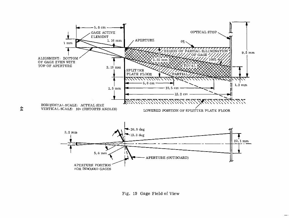
&kN?l. l$ mm 1 / APERTURE
ALIGNMENT: BOTTOM OF GAGE EVEN WITH TOP OF APERTURE
OPTICAL STOP, Ii-
~-n~-+?h-m~ HORIZONTAL SCALE: ACTUAL SIZE VERTICAL SCALE: 10x (DISTORTS ANGLES) LOWERED POSITION OF SPLIT/TER PLATE FLOOR
3.2 mm 26.8 deg
13.3 deg
22.1 mm --
- - - - - I--
APERTURE (OUTBOARD) e
APERTURE POSITION FOR INBOARD GAGES
Fig. 19 Gage Field of View

heating. This is visible on Fig. 32 where the 5 ,usec/cm sweep shows this event.
Most of the data were taken with the more convenient 2 psec/cm sweep and the timing
was such that this event was just off-scale.
4.3 THIN-FILM GAGE CONSTRUCTION
The platinum thin film heat transfer gages, used as thermal energy detectors for this
research, were constructed following the standard procedures described by Rabinowicz,
et al. , (Ref. 24) and will merely be outlined here.
The basic gage element was constructed on a fused quartz substrate approximately
4.8 x 2.5 x 1 mm thick as sketched in Fig. 20. The ends and a portion of the top
were painted with Hanovia Liquid Platinum Alloy 130-A (NEW) and baked following the
manufacturer’s instructions to provide means for attaching leads. A platinum strip
was then sputtered over the entire length of the gage creating an active element
1 x 3 mm as sketched. This element was then baked at 1100” F for 8 hr to age and
harden the film. It then had a resistance of 10 to 20 a and was slightly transparent
to visible light indicating a film thickness of less than 500 A. The element was then
glued to a convenient base, wires were soldered to the ends, and these solder joints
were painted with red Glyptal enamel.
PLATINUM PAINT
SPUTTERED PLATINUM
QUART Z SUBSTRATE
STRIP
Fig. 20 Basic Thin Film Gage Element
45

The next step for most gages was the evaporation of a dielectric layer of silicon
monoxide (SiO) for reasons to be discussed later. This was done in a 10 -5 Torr
vacuum using an Allen-Jones Electronics Corporation S13 chimney-type source at a
temperature nominally 1200” C. The gages were heated to 350°F and were located
5 in. away resulting in a deposition rate of about 1500 A/mm.
The last step was the application of a layer of aluminum black used as a blackening
agent. The aluminum black was applied in a manner quite similar to that used for
coating mirrors except that the evaporation was performed in a nitrogen atmosphere
at a pressure of 100 to 200 1-1. The result was a diffuse, black surface with a measured
absorptance of 0.98 f 0.01 in the visible and near IR spectrum. This coating was used
during the calibration of the silicon monoxide-coated gages but could not be used for
the shock tube measurements for reasons discussed in Sec. 4.6.
Gage Thermal Analysis. The thermal analysis of a thin film gage is essentially the
problem of one-dimensional transient heat conduction into a semi-infinite medium (i, e. ,
the quartz substrate). The inverse equation relating the surface temperature excess
T and the surface heat flux q is readily available in the literature [see Rabinowicz
et al. , (Ref. 24) or Vidal (Ref. 25)] and is
(4.1)
where k, p, and c P
are respectively the thermal conductivity, density, and specific
heat of the substrate, t is time and A is a dummy variable. This equation is appli-
cable to a thin film gage provided that the heat pulse does not completely penetrate the
substrate and provided the calorimetric effect of the thin film is small. It is well to
note here that q is the heat flux absorbed by the gage and not the flux incident on the
gage.
46

The surface temperature excess is determined by measuring the change of resistance
of the gage element. These are related by
R = RG(l + oT) (4.2)
where (Y is the temperature coefficient of resistivity of the sputtered platinum film.
A particularly convenient grouping of the gage physical properties is
(4.3)
because it will be shown below that this is the desired result of any gage calibration
procedure. Thus Eq. (4.1) can be written as
t 1 CYT = 2k’
I *dh. A=-x
(4.4) 0
For the special case of a constant heat flux, i, beginning at t = 0 this equation
becomes
(YT = $fi
4.4 GAGE BOX CIRCUIT ANALYSIS
(4.5)
The common method of determining a resistance change is to measure the voltage
change at constant current. This condition is approximated by the gage box circuit
shown in Fig. 21. Eight such gage boxes were used - one for each thin film gage in
the model. Typical component values are Eb = 6 V and I = 50 mA which requires
Rp to be about 100 a.
47

TO TEKTRONIX TYPE 2A61 DIFFERENTIAL AMPLIFIER @SPLAYS A-B)
O.l,uF
E
1 THIN FILM GAGE R =RG(l +aT)
Fig. 21 Schematic of Gage Box Circuit
The total (AC + DC) voltage across the gage is given by
EbRG(l + aT)
E = IR = Rp + RG(l + aT)
The AC component of this is
,e
I -
e = E(T) - E(0) = EbRp [Rp + RG][Rp + RG(l + aT)j (RG”T)
48

Now since crT is the order of 10 -6 or less, it is neglected in favor of unity in the
denominator whereupon the above equation reduces to
EbRp
e = (RP + RG)2 (RGcxT) = R IG:pRG (RG C~I’)
P (4.6)
where
IG = Eb
Rp + RG
The factor Rp/(Rp + RG) accounts for slight variations in the gage current and should
be included unless, of course, Rp >> RG .
Now combining Eqs. (4.4) and (4.6) results in
e =IR RpL G GRp+ RG2k’ I
0
and defining a calibration constant as
K = k’(R + RG)
IRR GGP
yields
e
49
(4.7)
(4.8)

.
For the special case of a constant heat flux, q , beginning at t = 0 , this equation
reduces to
ij = K$-
Equation (4.7) can be rewritten as
ICK = g G
4.9)
(4.10)
and we note that k’ is a property of the gage itself [ Eq. (4.3)] and that the factor
1 + R /R G P
is relatively insensitive to changes in R P since RP ’ R G’ Now because
a significant change in RG is sufficient reason to discard a gage, the product IGK
tends also to be a property of the gage and this fact was used in the data reduction to
account for slight (10%) changes in IG caused by battery aging or different values of
Rp in the various gage box circuits.
4.5 DATA REDUCTION
The first part of the data reduction procedure consists of obtaining the unknown heat-
flux history q(t) from a given arbitrary voltage signal e(t). If the time variation of
q(t) is known, then Eq. (4.8) may be integrated as for example in Eq. (4.9). Several
forms of the inverse of Eq. (4.8) [where q(t) is given explicitly in terms of e(h)] are
given by Vidal (Ref. 25), but this approach eventually results in the same kind of
mathematical manipulations as in the approach below.
The approach taken was to assume that the heat flux varied linearily over any arbitrarily
small (but uniform for simplicity) time interval 6t and further was continuous. This
assumption is in accord with the expected radiative history in the reflected shock region
(including the starting transient).
50

Defining a reduced, heat flux by
q*(t) = q$)
the assumed variation is given by
c(t) = a,(t - tm) + bm for tm ‘5 t I t
m + 6t
tm = m6t
m = 0,1,2,...
Continuity is given by
bm = am-l6t + bm-l m = 1,2,3 ,...
and b. is arbitrary.
At this, point inserting the above relations into Eq. (4.8) results in a sum of m
integrable integrals. The solution now becomes a matter of algebraic manipulations
and keeping track of the special cases for small m . The continuity relation allows
one to build up the solution because the heat flux at any point in time depends on pre-
vious history. Introducing the shorthand notation qm = q(t = tm) , the solution at
the discrete times tm = m 6t is given by:
4 = arbitrary (usually zero for experimental traces)
* 3 e(t,) q1= -- 2d-z
-+ci,
* 3 W,) 92 = --- - - -
2m 2(fi 1,q; ( 1 $ > q;
51

~=g!& phi7 q* - (m)3’2 (q; - q*) + 2qmm1 - G-2 0 0
m-l
-1 (m-n+l)3’2(<-241*1-l+< 2) m = 3,4,5 ,...
n=2
This system of equations has been programmed for an IBM 7094 digital computer.
The e(t,) input data is read from a Polaroid photograph of the oscilloscope display
of the gage output voltage. Ordinarily twenty to thirty input data points are read. An
initial condition on Eq. (4. 1) is that the surface temperature (and hence the AC output
voltage) must be zero at time zero. Thus the time origin must be chosen so that at
least the initial voltage is zero.
The computer output format included a plot of both the output and the input on the same
graph. Examples of these will be found in later sections of the report.
The heat flux absorbed by the gage, q , is related to the intensity at the gage, I , by
the following relation
% I=w=A ii Ap cos e/p2
(4. 11)
because the dimensions of the aperture are small compared to the separation distance,
P* Here A P
is the area of the aperture, 8 the angle between the line p and the
normal to the aperture (the gages were installed normal to this line), and G a
weighted gage absorptance defined by
(4. 12)
52

As discussed earlier in this report, it was decided to include the absorptance in the
theoretical predictions of the intensity so that the above equations might well be written
cyvIv dv = E;I =
0
(4. 13)
where each term represents the intensity insofar as the data reduction procedure is
concerned. The bracketed factor represents the solid angle subtended by the aperture
and was nominally 2 x 10 -3 sr (A P
= 1.2 X 5.6 mm, p = 5.6 cm, 8 = 13 or 26 deg).
4.6 GAGE CALIBRATION - HEAT LAMP
The thin film gages were calibrated by two independent methods - one using a heat
lamp and the other an electrical bridge circuit. In the heat lamp method a gage was
exposed to a radiation pulse of known intensity and the aforementioned computer pro-
gram used to calculate K .
This method requires that the absorptance of the gage surface be known. Because the
lamp radiation was mostly in the visible and near infrared spectral region where the
surface absorptance of the SO-coated gages varied (Fig. ll), a coating of aluminum
black was evaporated on the surface of these gages. This coating was adequate for
the 20 msec time scale of a lamp calibration but it was thermally thick and could not
be used for the shock tube measurements where the time scale was about 10 ,usec.
Fortunately metallic black coatings are quite easily removed. It was relatively simple
to apply a thermally thin layer of aluminum black to a bare platinum gage element and
thus this coating was used for both calibration and shock tube measurements for this
type of gage.
A schematic of the lamp calibration apparatus is shown by Fig. 22. The heat lamp
was a commercial quartz lamp with a gold plated reflector. The water cell filter
blocked much of the IR radiation and the aperture provided a reference point for gage
53

HEAT LAMP
MENISCUS LENS
WATER CELL FILTER
SHUTTER
APERTURE
THIN FILM GAGE
PHOTOTUBE MONITOR OF HEAT PULSE
OUTPUT OF GAGE 282
Fig. 22 Heat Lamp Calibration Apparatus and Typical Output Traces

location. The radiant flux at this aperture was measured with three different U. S.
Navy Radiological Defense Laboratory slug-type calorimeters and was found to be
2.52 W/cm2 after a 2-set lamp warm-up.
A typical gage output trace is shown by Fig. 22 together with a phototube monitor of
the heat pulse. Figure 23 shows the output of the computer program for this same
gage. The ordinate is q* = q/K for the solid curve. The time variation agrees well
with the phototube monitor and since the constant portion of the absorbed heat flux is
0.98 (2.52) W/cm2, the calibration constant is obtained directly as shown.
The heat lamp calibration subjected the gages to a heat pulse about 10% of the actual
shock tube values and this occurred over a time scale 2000 times longer. The result
was an output signal voltage (or aT product) about four times that realized in the
shock tube.
4.7 GAGE CALIBRATION.- BRIDGE
The second and independent calibration method used was to heat the gage internally by
the Joule heating from a current pulse passing through the sputtered platinum element.
This requires a bridge circuit to separate the large steady heating voltage from the
small signal caused by the gage element temperature (and hence resistance) change.
The bridge calibration could easily simulate the experimental heat fluxes over a time
scale about five times longer. This method is independent because the analysis
requires an entirely different set of assumptions and measurement parameters and
hence provides an absolute check on the validity of the lamp calibration.
The analysis of the bridge calibration will utilize the smaller schematic of Fig. 24
which includes the salient features of the actual circuit. Here the bridge as drawn is
initially balanced because balancing is relatively simple to do on the actual circuit.
Although it is not essential that both legs be identical, this will prove to be useful
feature .
55

-- - - 0.024
0.023 -
0.022 -
0.021-
0.020 -
0.019 -
0.018 -
0.017 -
0.016 -
0.015 -
0.014-
3 0.013-
0.012 -
O.Oll-
0.010 -
0.009 -
0.008-
0.007 -
0.006 -
0.005 -
0.004 -
0.003 -
0.002 -
O.OOl-
X
0 COMPUTEROUTPUT, q/K
X INPUTVOLTAGEPOINTS (SCALENOTSHOWN)
K - 9 _ 10.98)(2.52) q/K 0.0244 = 101
X
0. 0 I I I I I 1 -~-A---J 0 2000 4000 6000 8000 10,000 12,000 14,000 16,000
SWEEP TIME (psec)
Fig. 23 Computer Output for Gage No. 282
56

Eb (32-250 V)
P 1.2K
TO DELAY PULSE
.ED4 2D21 44
I 100.5 (8 W)
A /dk,,,W) \7.,,,W)
250 pF
THIN FILM
(RESISTANCE RG)
I PREAMPLIFIER OF OSCILLOSCOPE (DISPLAYS A-B)
*RESISTANCE SELECTED TO BE SLIGHTLY LARGER
r
THAN RG
t=o R
P
+
‘,Eb F
T- SALIENT PORTIONS OF CIRCUIT
Fig. 24 Bridge Calibration Circuit
57

The following expressions for the current in each leg may be derived in a straight-
forward manner:
I = Eb(R1 + RG)
Rp(R1 + RG) + (RI + RG + Rp)(Rl + R,
IL = Eb(R1 + RI
Rp(R1 + RG) + (RI + RG + RP) (RI + R)
The differential output voltage, e. is given by
e 0
= I.3 - ILRG
and by neglecting CJJT (of order 10S6) in favor of 1 + RI/RG (can be made of order 10)
in the denominator, we get upon eliminating the currents and simplifying
e 0
The power dissipated in the gage is given by
2 p = 12R =
EbRG(l + cuT)
(RI + RG + 2Rp)2
(4.14)
(4.15)
where the denominator has been simplified using the above argument. But here it is
consistent to neglect the (cxT) product in the numerator in favor of unity with the
result that the power dissipation is essentially constant. Noting that q .= P/A (where
A is the area of the gage element) provided that the sputtered film is uniform (more
will be said about this shortly), we now have a condition of constant heat flux and
Eq. (4.5) is applicable.
58

1 Substituting Eqs. (4.14) and (4.15) into Eq. (4.5) yields
(4.16)
where
p = ~~ (Eb13R1 A(RI + RG)(R1 + RG + 2Rp)3
Bymaking Rl>RG, the factor 6 becomes a very weak function of RG and so is
readily tabulated for a given R P’
a nominal A , and certain fixed values of E b’
The actual bridge circuit is also shown in Fig. 24. The large energy storage capacitor
maintains a constant voltage over the 80+sec test period. Switching is accomplished
by actuating the mercury wetted contact relay which closes in nanoseconds. It is
necessary to terminate the current pulse to prevent possible overheating and destruc-
tion of the gage. This is accomplished by firing the thyratron 80 psec or so after the
relay is closed by using a delay generator.
No inductance problems were encountered in building the bridge and composition
resistors were used throughout. The performance of the entire bridge was checked
using a bifilar-wound (low inductance) nichrome (a! essentially zero) resistor in
place of a gage and the expected zero trace was achieved.
It is difficult to measure RG directly because of the attendant heating that must occur.
This measurement is easily done on the balanced bridge by removing the gage and
measuring the value of the adjustable resistors in the other leg. It can be shown that
a bridge unbalance of 0.01 Q will result in a zero shift of 1.5 mV at Eb = 125 V and
such a zero shift is readily noticed.
59

An example of a typical bridge calibration is shown in Fig. 25. The inset shows the
actual oscilloscope trace from which eight points were read and plotted versus the
square root of time. The linearity of the plotted points proves that the output voltage
had the parabolic behavior indicative of a constant heat flux [ Eq. (4.5)] and,the bridge
was properly balanced because an extrapolation of the data points will fall quite near
I the plot origin.
The bridge calibration is amenable to checking the linearity of the gages because the
simulated heat flux is readily varied over a wide range by merely changing Eb . A
typical result of a linearity check on a gage was that k’ varied by about l 2% over a
simulated heat flux range of 5 to 42 W/cm:!. No linearity problems were anticipated
because the experimental heat fluxes were never large enough to cause a 1°C rise in
gage surface temperature in the available test time.
4.8 COMPARISON OF GAGE CALIBRATION RESULTS
A comparison of the results of the heat lamp and bridge calibration for eighteen gages
is given in the upper half of Fig. 26. Here we note that while the results for six gages
agree within & 5% and five more agree within + 12%) the remaining seven all show a
rather large, one-sided discrepancy. The lower half of Fig. 26 shows the lamp results
and it is seen that these are fairly consistent and the average is somewhat less than
twice the value calculated using handbook bulk property values - a common occurrence
with sputtered platinum thin film gages. Thus it would appear that the lamp calibra-
tion is correct and that the discrepancy lies in the results obtained from the bridge
calibration.
This discrepancy is explained by considering the effect of a non-uniform gage element
in both calibration methods. The bridge is especially susceptible to effects caused by
non-uniformities in the sputtered film because here the local heating depends on the
local resistance. A microscopic examination of many gage elements revealed that
occasionally the sputtered platinum film tended to pull away or thin out at the ends of
60

Fig. 25
I THYRATRON FIRES - I
5 AMPLIFIER ‘;’ TRANSIENT
GAGE NO. 140 RG = 20.38 SZ Eb = 125.0 V
A = 0.033 cm2
SLOPE = 0.663 mV/G SLOPE = 0.663 mV/G p = 152.7 mV W/cm2 p = 152.7 mV W/cm2
k, = 152.7 X (20. 38)2 k, = 152.7 X (20. 38)2 0.663 0.663
= 0.96 x lo5 "7 = 0.96 x lo5 “7 cm cm
SIMULATED HEAT FLUX = 18.5 W/cm2 SIMULATED HEAT FLUX = 18.5 W/cm2
Example of Bridge Calibration Including Actual Oscilloscope Trace and Data Reduction
61

1. 0 1
0.8
1.2
1.0
0.8
0.6
H
-k l fH
HHHH HHHH HH
H#+
-----
0.4 ,’ k
------mm -- ---
I
‘VALUECALCULATEDFROMHANDBOOK
0.2 - BULK PROPERTY VALUES
t
GAGE
Fig. 26 Comparison of Results of Lamp and Bridge Calibration
62

the active element during the aging process. A general analysis of the bridge calibra-
tion method for a non-uniform gage is tedious and it will suffice here to postulate that
the gage element consists of two parts differing in resistance and area.
We assume that the gage active element consists of two parts, a and b , that are
electrically in series so that the total gage resistance is given by
R = R,(l + aT)a + Rb(l + aT)b = RG + (FM), + (RQT)~ (4.17)
where
RG =Ra+R b
The analysis of the effect of a two-part gage on the bridge calibration is quite similar
to that done earlier and the result is
e 0 = (Ebj3 R R: R JT
1 G (R1 + RG + 2Rp) 3 [(@a + (jgb]
Now we further assume that the physical constant, k’ , is identical in both parts. This
is reasonable considering the relative constancy in the lamp calibration results for
many gages. The above expression becomes
k’ = * [(5-Ja + (qb] where p is given by Eq. (4. 16). By introducing
R A R* = 2 , A* = 2 where A = Aa & %
RG
63

the above expression becomes
P(RG)’ k’=v 1
J (4.18)
and except for the factor in brackets, this equation is identical to Eq. (4. 16), the
corresponding result for a uniform gage. Since the bridge calibration method tacitly
assumed a uniform gage, this bracketed factor represents an unknown correction that
should have been applied, but was not. This factor has a minimum value of unity for
A* = R* (i. e., a uniform gage) and is greater than unity for all other possible values
of A* and R* between zero and unity. A thin spot in the sputtered film would mean
that it is possible for a large fraction of the resistance to occur over a relatively small
fraction of the total area and hence the bracketed factor could easily be as large as a
factor of two. Thus any amount of gag,e non-uniformity will make the value of k’
obtained by the bridge calibration too small. A reduction in k’ by one-half is not
unreasonable.
The results of the lamp calibration are not affected by a non-uniform gage element.
This can be proven by using Eq. (4.17) instead of Eq. (4.2) in the gage box circuit
analysis and again assuming that the physical constant k’ is identical in both parts.
We will not go through the equations here because a logical argument will yield the
same result.
The heating of the gage surface in the lamp method is uniform even though the gage
resistance is not because here the heat source is external to the gage and not the gage
element itself as it is in the bridge method. Thus the surface temperature rise of
each part of the gage is identical [ Eq. (4. l)] and the parts act in series. If k’ is
identical then all the equations in the gage box circuit analysis are unchanged and hence
the lamp calibration is valid. Even if the values of k’ were different, there would be
no effect in the data reduction procedure. Admittedly Eq. (4. 10) would no longer hold,
but one could merely treat Eq. (4.8) as the defining equation for K and since the heating
64

mode is the same in both the lamp calibration and the-shock tube experiments, the
data reduction procedures using the K so defined would be valid.
Thus the conclusion is reached that the discrepancy in the comparison of the gage
calibration results stems from uncorrected gage non-uniformities which caused the
bridge results to be too low while having no important effect on the lamp calibration
results and no effect on the data reduction provided (as was done) the heat lamp cali-
bration results are used. These conclusions are borne out by Fig. 26.
The bridge calibration was employed as an independent check on the lamp calibration
and since from Fig. 26 the values of k’ lamp’kbridge are either essentially unity or
greater, the absolute validity of the lamp calibration is verified. The bridge calibra-
tion is still a valid gage linearity check because the unknown factor of Eq. (4. 18) is
not a function of the magnitude of Joule heating but rather its distribution.
4.9 GAGE TIME RESPONSE CHECK
The only yet unsolved facet of the gage calibration procedures is a check of the time
response since the time scales used in the lamp and bridge calibrations were both
greater than that used in the shock tube.
The gage time response was obtained by irradiation with a 15-,usec pulse of visible
light obtained from a xenon flash tube. The gage output was fed into the computer
data reduction program and the computer output compared against the pulse shape
obtained using a photomultiplier tube. Examples of this are given by Figs. 27 and 28
where the solid lines are the computer output while the dashed lines are the normalized
pulse shape plotted on the same time scale. Figure 27 shows the time response of a
bare gage (i. e. , no coating on the platinum element) and here the pulse shape is
reproduced quite well with a time lag of about 1 psec. Since this time is equivalent to
the risetime of the oscilloscope differential amplifiers, it is considered quite accept-
able. Figure 28 shows the results of a gage coated with a 4-min evaporation of SiO
and which exhibited the largest time lag of a number of gages with various coatings.
65

26C
24C
22c
20(
18(
Ii- ' 16C
%
-2 140
z
g 120
100
80
60
40
20
\\ 1 X
X X x \ x
X X ' xx
X X \ \ .
X
X
X X
\
0 COMPUTEROUTPUT
I I I I I I I I I 2 4 6 8 10 12 14 16 18 20 22 24
SWEEP TIME (,usec)
X INPUTVOLTAGE POINTS (SCALENOTSHOWN)
Fig. 27 Xenon Flash Results for Bare Gage
66

-1 --11 I I I I I I 480 p\
460 / /
440 -
420 -
400 -
380 -
360 -
340 -
320 - z yl 300-
wfj 280-
5 260 -
z 240-
E 220- lx g 200- Y
180 -
160 -
140 -
120 -
100 -
80 -
60 -
40 -
20 -
O& 0
X
X
X
/ I -1.. --L -~ .I 2 4 6 8 10
-
XENONFLASH \ ENVELOPE b\
X x\x X
X \
X \
\ X \
X \
\
\
\
\
0 COMPUTEROUTPUT \ \
x INPUTVOLTAGE POINTS .s (SCALE NOT SHOWN)
I -I-- I I I I I 12 14 16 18 20 22 24
SWEEP TIME (psec)
Fig. 28 Xenon Flash Results for Gage With 4 min. of Silicon Monoxide
67

Here the delay is about 2 or 3 psec and some distortion of the pulse shape is apparent.
However, this is not serious when compared to the 15-psec test time and such per-
formance was considered acceptable.
An EG&G.FX-12 xenon flash tube was pulsed by using a lumped parameter delay line
with a total energy storage of 1.4 J (8 pF, 600 V). No circuit schematic is given here
because the required parameters vary with individual flash tubes and tube life and one
must resort to trial and error adjustments to obtain the desired pulse shape. The
flash tube light output was gathered by a parabolic mirror and concentrated by a con-
densing lens with the result that the peak heat flux was about 500 W/cm2. This flux
varied from flash to flash and so this time response check was not used as a calibra-
tion method. This variation could be minimized by increasing the total energy in the
delay line but at a considerable sacrifice in flash tube life.
4.10 NOISE PROBLEMS
Noise is a perennial problem in any experimental investigation and this research was
no exception. Several noise sources were identified and eliminated while at least one
other source was suppressed but not entirely eliminated. The noise problems can be
divided into two areas: those that occurred when windows were used and those which
occurred only when no windows were used. We shall logically begin with the former.
The effects of one large and erratic noise source are given by Fig. 29 which shows
noise traces from three thin film gage channels together with a sketch of the model
configuration at that time. A copper disc was used instead of a window to ensure that
no radiation or test gas entered the gage cavity. The noise on the three traces cor-
related quite well with the incident shock position as shown in the figure. The impor-
tant thing to note is that there was no noise associated with event D - the time when
the incident shock struck the splitter plate floor. Noting that this was the only event
where the incident shock reflected back uniformly, it was suspected that the noise was
caused by magnetic pickup from vortices generated by asymmetries in the flow. It
might be added that the thin film gages and associated circuitry were already supposedly
well-shielded magnetically with Netic and Co-Netic metal.
68

CHANNEL
3
5
6
VERTICAL SENSITIVITY (mV/cm)
0.2
0.2
0.5
EVENT A : SHOCK STRIKES EVENT C : SHOCK STRIKES EVENT D : SHOCK STRIKES EVENT E : SHOCK STRIKES
A CD E
SHOT: 284 WINDOW: COPPER (NO TEST GAS OR RADIATION
ENTERED GAGE CAVITY)
Fig. 29 Correlation of Noise Traces With Incident Shock Position
69

The solution was to mount a ring around the model in the manner sketched in Fig. 30
to stop the flow uniformly in the region outside the splitter plates. The results are
shown in the upper-half of Fig. 30 where a dramatic noise reduction was realized.
Later in the experiment some erratic noise became evident in the traces at event D
when higher (to 50 pV/cm) oscilloscope gains were used. These were cured by physi-
cally relocating the gage circuit cable connectors to a point where they could be mag-
netically shielded more effectively. At this time the noise level of the thin film traces
was reduced to a value very nearly the inherent preamplifier noise. This is shown by
Fig. 31 which shows traces from six channels during one of the last window shots. The
missing two channels were off-scale as a result of an occasional disturbance from the
trigger bank of the arc tube driver which was later completely eliminated by reducing
the current loops in the trigger bank circuit.
Thus it is concluded that the noise caused by magnetic pickup was greatly reduced by a
model designed to eliminate asymmetries in the flow but that careful attention to magnetic
shielding was still necessary to eliminate the erratic vestige that remained at very high
instrumentation gains. It was not necessary to employ the SiO dielectric layer for gages
used behind a window and indeed over half of the window data presented in the next sec-
tion was taken with the aluminum black on platinum type of gage.
We now turn our attention to the noise problems uniquely associated with the model in
a windowless configuration and Fig. 32 is indicative of the early noise problems. Here
it is seen that only one channel (Channel 4) appears acceptable while the other seven
all show varying degrees of excessive noise. The traces of Channels 1, 3, and 8 went
completely off-scale at the time the incident shock struck the bottom of the splitter
plates (event D of Fig. 29) and this is also the initial time when radiation from the
reflected shock region was incident on the gages. The gains of 0.5 to 2.0 mV/cm
were at least ten times less sensitive than the maximum gains ultimately employed.
Heretofore the effectiveness of the SiO insulation was determined by dipping the gage
into mercury and measuring the resistance to the active element. This provided no
70

I’
VERTICAL SENSITIVITY CHANNEL (mV/cm
1 0.2)
2 0.2 I
3 0.2 I
5 0.2 I 6 1.0 f
7 1.0
8 0.2 I
A SHOCK STRIKES B SHOCK STRIKES
RING POSITION ---- ----
SHOT: 285 WINDOW: COPPER (NO TEST GAS OR RADIATION
ENTERED GAGE CAVITY)
Fig. 30 Noise Traces After Addition of Ring
71

CHANNEL
2 (OFF SCALE)
4 (OFF SCALE)
CAVITY PROFILE
-+I I-- 2 ,usec, ALL SWEEPS
SHOT 355, MS = 25.2 , P1 = 200 p
ALL GAGE CHANNELS AT 50 pV/cm
Fig. 31 Examples of Traces Obtained Behind Suprasil Window
72

VERTICAL SENSITIVITY CHANNEL (mV/cm)
1 1.0
2 0. 5
3
4
8
2.0
1. 0
0.5
1. 0
1. 0
0.5
SHOT: 288 WINDOW: NONE
I
TEST GAS HITS
l-
‘-+ +wec
EVENT D
Fig. 32 Examples of Traces Obtained Without Window
73

information about pinholes or fissures in the SiO layer because the mercury did not
wet this layer. Therefore a plasma check, shown schematically by Fig. 33, was
instigated to. provide a more meaningful test. The method of performing this check
was to determine the plasma potential of the gage (i. e. , the voltage at I = 0, typi-
cally -10 V) and then to bias the gage more positive and note the current.
The results of this plasma check on the gages used in Shot 288 (Fig. 32) were as
follows :
l The gages in all channels except Channel 4 drew 10 to 70 times as much
current as Channel 4 when biased + 10 V from their plasma potential.
l The gages corresponding to the traces that showed high frequency noise
(Channels 1, 2, 5, and 6) were erratic during the plasma check.
At this time these results indicated that the plasma check could determine the effective-
ness of the SiO insulation and hence the SiO evaporation procedure was much modified
until gages that drew less than 5 X 10 -9 A at 12-V bias were commonplace. The final
evaporation procedure was the one already described.
Unfortunately only about 20% of the gages of this generation yielded relatively noise-
free traces in the windowless model at the higher (to 50 c.lV/cm) oscilloscope gains
ultimately employed. Therefore, the plasma check must be considered as a necessary
but not sufficient test. This then is the state of the art at the time of this writing.
Many unsuccessful attempts were made to correlate the construction details or varia-
tion of the SiO evaporation parameters. These parameters included source tempera-
ture, separation distance, evaporation time and two separate evaporations (an artifice
used to minimize pinholes caused by foreign materials). No notable improvement in
this 20% acceptance figure was realized during any of these perturbations.
Further the gages in general were not durable and often a steady increase in noise was
experienced. Some lasted for only several shots while a few yielded consistently good
results for a dozen shots or more. Many gage failures were attributed to a separation
74

r -mm--------- 1
I I I I I I I I L-
ALUMINUM CATHODE s
)
I BELL JAR
I
f
’ P = 125 p m I
I GLOW DISCHARGE
7 Ii .I+ I
GAGB GAGB I I
I I t ALUMINUM
ANODE I I
I I
INSULATION INSULATION I I -mm-- I- ---s---
1,
I ELECTRON FLOW
l d---- 20mA
50K
HV -1500 v
POWER SUPPLY
I A
ESV VTVM VTVM
Fig. 33 Schematic of Plasma Insulation Check Apparatus Fig. 33 Schematic of Plasma Insulation Check Apparatus
75 75

of the SiO and the platinum from the quartz substrate. Before the SiO evaporation the
sputtered platinum film was hard and could be removed only with great difficulty, but
after the SiO evaporation the film was rather easily removed by scraping with a sharp
instrument. Possible causes for this degradation include stresses caused by the con-
densing SiO, free silicon embrittlement of the platinum, or as was suggested, reduc-
tion of an intermediate platinum oxide compound which provided the initial strong
bonding. Therefore, while this state of the art leaves something to be desired, never-
theless by building many gages and subjecting each one to a final test in the shock tube
it was possible to obtain meaningful results. Figure 34 shows examples of gage traces
that yielded good data in the windowless model. We now turn to a discussion and possi-
ble explanation of the noise source(s) of the 80% of the gages that were rejected.
Figure 35 shows examples of the traces from rejected gages in the windowless model.
The top five traces indicate the common initially-negative behavior while the bottom
two show the opposite and much less oommon initially-positive noise bump. All these
bumps occurred at the time the incident shock struck the floor of the splitter plates
and one would suspect that they were caused either by some interaction with the
ionized gas in the gage cavity at PI or by some residual magnetic pickup. The latter
was eliminated by noting that this behavior was not seen when windows were used and
further was cured several times by merely painting the surface of the rejected gage
with red Glyptal enamel and observing the noise trace on the ensuing shot.
The gas in the gage cavity becomes ionized by photoionization at the onset of radiation
as a result of the vacuum ultraviolet radiation that was formerly blocked by the
Suprasil window. That the gas becomes ionized at this time was proven by placing
two small plates at the gage location and about 1 cm apart. With 22 V across the
plates, several milliamperes of current were drawn at a time beginning when the
incident shock struck the floor of the splitter plates. Also this is the time when
faulty gages went off-scale (Channels 1, 3, and 8 of Fig. 32). Therefore the gages
must operate in a transient, room-temperature plasma while exposed to vacuum
ultraviolet radiation. This is the essence of the windowless problem and because it
is a difficult situation to create in a bench-type experiment, one must resort to a trial
and error experimentation in the shock tube itself.
76

GAIN SHOT CHANNEL (mV/cm)
291
292
2 0.2
3 0.2
304 8 0.2
308 4 0.2
310 6 0.2
342 5 0.2
359 6 0. 1
366 6 0.1
373 5 0. 1
Fig. 34 Examples of Traces From Acceptable Gages in the Windowless Model
77

GAIN SHOT CHANNEL (mV/cm)
309 6 0.2
315 5 0.2
357 1 0.1
367 4 0.05
373 1
342 6 0.2
0.05
376 5 0.1
/
/ -- + +- 2 t--c
Fig. 35 Examples of Traces From Rejected Gages in the Windowless Model
78

The windowless noise phenomena discussed above are not unique to this experiment
and several authors have expressed their views on the subject; Gaydon and Hurle
(Ref. 26 ) note this effect when thin film gages are exposed to an ionized flow and con-
clude that the initially-negative behavior is caused by charge acquisitian rather than a
shorting effect. In a similar situation Marrone and Hartunian (Ref. 27 ) considered
the problem as a shorting effect and cured it. by an evaporated layer of SiO. It is noted
here that a 0.1 rn* negative signal could be caused by a decrease in gage resistance of
only 0.01% for a 20-Q gage at 50 mA and this corresponds to suddenly paralleling the
gage with 200 kQ.
Clearly more work needs to be done on the problem of making total radiation measure-
ments (including the vacuum ultraviolet) in a transient and cold plasma.
79

Section 5
DISCUSSION OF RESULTS
Experimental radiative intensity data have been obtained at two shock tube conditions.
These conditions are (1) T = 14,70O”K, p/p, = 3.18 x 10m2
g/cm3.
where p, = 1.29 x 1o-3
At the first condition, data were obtained with and without a window and also
with a window in combination with a filter which transmits only in the infrared. At
the second condition data were obtained with and without a window. The data are pre-
sented in Figs. 36 through 40. The test conditions in the shock tube were difficult to
control precisely and the data presented in these figures were adjusted to the tempera-
ture indicated on the respective figures. The adjustment to the data were made accord-
ing to the variation in intensity with temperature as indicated by the results in Fig. 5.
Any data which required an adjustment greater than 50% were not considered. The
adjustment to the data on the average was about 15%.
The data obtained behind a window at the first test condition are presented in Fig. 36.
The transmission curve for the window used to obtain these data is presented in Fig. 14.
The data presented in Fig. 36 were obtained with three different model configurations.
The first condition is the normal one as depicted in Fig. 19. For the second condition
the floor plate was lowered by 0. 10 in. The reason for lowering the floor plate was
to check the possible effect of truncating the field of view of the gages and possible
cooling of the test gas by conduction to the floor plate. Lowering the floor plate
decreases both the field of view truncation and thermal cooling. For the third condi-
tion the plate was kept in the lowered position and the quartz window at the aperture
was moved back and placed immediately in front of the gage. With this configuration
it was possible to obtain data behind a window with the gas expanding into the cavity.
A comparison of the data obtained with this configuration to the data obtained with the
original configuration provides an experimental check on the effect of expansion wave
in the test gas. The effect of field of view truncation, thermal cooling, and the
80

/
0
/ ’ *
i, 8 0 V
d 8
/+
/f-----CONTINUUM ONLY
I 0 0 DATA WITH FLOOR PLATE IN ORIGINAL POSITION
I
z i- DATA WITH PLATE LOWERED 0.10 in.
v DATA WITH PLATE LOWERED 0.10 in. AND WITH + WINDOW AT GAGE
U 2 4 6 8 10 12
GEOMETRIC PATH LENGTH, 6 (cm)
Fig. 36 Radiant Intensity Data Obtained Behind a Quartz Window: T = 14,700”K P/P, = 3.45 x 10⁻²
81

propagation of the expansion wave into the test gas is not discernable in the data pre-
sented in Fig. 36. From these results it is concluded that the above effects are not
important with the present data scatter.
The gages used to obtain these data were coated with aluminum black so that the sur-
face absorption was uniform and at a value of approximately 0.98. The continuum
prediction was obtained from Fig. 12 while the line prediction was obtained from
Fig. lob. A comparison of the theoretical prediction of the lines plus continuum
intensity show that the predictions are approximately a factor of two higher than the
data. On the other hand, the continuum only prediction is in good agreement with the
data. The variation of the intensity data with geometric path length is in good agree-
ment with the prediction. Furthermore, the intensity variation is nearly linear which
indicates that for the frequencies transmitted by the window, the gas is optically thin.
The discrepancy between the theoretical prediction and the experimental data was
consistently present in all of the data obtained (Figs. 36 through 40). Possible
reasons for this discrepancy will be discussed later.
In Fig. 37 are presented data which were obtained behind a window in series with a
filter. The transmission of the filter is shown in Fig. 14. The corresponding
theoretical predictions were obtained by taking into account the transmission charac-
teristics of both the window and the filter. Again, it is seen that the data are somewhat
below the lines plus continuum prediction.
Data obtained without a window are presented in Fig. 38. As the geometric path length
is increased the data increases and then apparently levels off. At the present time it
is believed that the data at the longer path lengths (1 > 9 cm) are not valid through no
explanation can be offered at this time. The data obtained at the shorter path lengths
are seen to be in better agreement with the continuum only prediction than the total
lines plus continuum prediction. These predictions employed the surface absorptance
values presented in Fig. 11 (No. 2). A comparison of the windowless data with the
window data of Fig. 36 shows the importance of the vacuum ultraviolet. The nonlinear
behavior of the intensity with the geometric path length indicates the importance of
self absorption.
82

5 x lo2
CONTINUUM ONLY CONTINUUM ONLY
0 DATA WITH FLOOR PLATE IN ORIGINAL POSITION 0 DATA WITH FLOOR PLATE IN ORIGINAL POSITION
I -I- DATA WITH PLATE LOWERED 0.10 in.
0 2 4 6 8 10 12 GEOMETRIC PATH LENGTH, 6 (cm)
Fig. 37 Radiant Intensity Obtained Behind a Quartz Window and Filter: T = 14,700” K P/P, = 3.45 x 10⁻²
83

CONTINUUM
8
/ / 0 0 /o “/ / 0 8 8 8
I
/ - CONTINUUM ONLY
/
/O
/
/
I 0
I
I
I O
I I I I 0 2 4 6 8 10 12
GEOMETRIC PATH LENGTH (cm)
Fig. 38 Radiant Intensity Obtained Without a Window: T = 14,700”K; P/P, = 3.45 x 10⁻²
84

Similar window and windowless data for the second shock tube test condition are pre-
sented in Figs. 39 and 40. The window data are in good agreement with the continuum
only prediction. The windowless data at the long path lengths appear to be somewhat
low. The total theoretical prediction for this case is consistently higher than the data.
A comparison of the window and windowless again indicates the importance of the
vacuum ultraviolet.
There are several possibilities for explaining the discrepancies between the data and
the theoretical predictions. The first is that the shock tube temperatures are some-
what lower than those obtained from the shock tube using the measured value of the
incident shock speed. If the gas temperature is approximately 5 to 7% lower than the
values given by the shock tube tables, the agreement between theory and data would
be quite good. The possibility that the temperature of the gas in the reflected shock
region is less than expected is currently being examined. An alternate explanation to
explain the discrepancy between theory and data is that the line radiation is over-
predicted. As discussed in Sec. 3.2, there is considerable uncertainty on the half-
widths of the line profiles. This uncertainty in the half-widths and the oscillator
strengths results in uncertainties in the line radiation predictions of about 30 to 50%.
It is currently thought that the line predictions may be too high but the uncertainty in
the line prediction is not large enough to account for the discrepancy between theory
and experiment.
85

2x 10’
104
2 x lo3
LINES PLUS CONTINUU
/h- CONTINUUM ONLY
/
I I
0 2 4 6 8 10 12
GEOMETRIC PATH LENGTH, 6 (cm)
Fig. 39 Radiant Intensity Data Obtained Behind a Quartz Window: T = 17,OOO”K; p/p, = 3.18 x 1O-2
86

LINES PLUS CONTINUUM
CONTINUUM ONLY
/ 0
0 0
0 /
8
0
/ 0
0
104
/
0 0 0
I
Oo O 0 8
8
0
0
0 I I I I I I
I 2 4 6 8 10 12
GEOMETRIC PATH LENGTH, 6 (cm)
Fig. 40 Radiant Intensity Data Obtained Without a Window: T = 17,000” K; P/P, = 3.18 x 1O-2
87

Section 6
CONC LUSIONS
From the results of this investigation we conclude first of all that the vacuum ultra-
violet is a significant contributor to the integrated radiative heating to entry vehicles.
Secondly, we conclude that self-absorption is an important mechanism in reducing the
radiative heating. Finally, we conclude that our present knowledge of radiative energy
transfer is such that we can predict the integrated intensity to within a factor of two.
Although this is a significant improvement to the order of magnitude uncertainty
which existed previously, additional theoretical and experimental work is necessary
to reduce this uncertainty to acceptable levels.
88
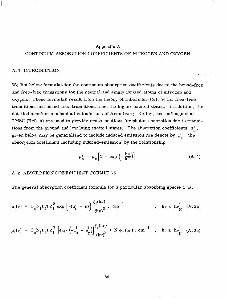
Appendix A
CONTINUUM ABSORPTION COEFFICIENTS OF NITROGEN AND OXYGEN
A. 1 INTRODUCTION
We list below formulas for the continuum absorption coefficients due to the bound-free
and free-free transitions for the neutral and singly ionized atoms of nitrogen and
oxygen. These formulas result from the theory of Biberman (Ref. 9) for free-free
transitions and bound-free transitions from the higher excited states. In addition, the
detailed quantum mechanical calculations of Armstrong, Kelley, and colleagues at
LMSC (Ref. 3) are used to provide cross-sections for photon absorption due to transi-
tions from the ground and low lying excited states. The absorption coefficients ph,
given below may be generalized to include induced emission (we denote by PC, the
absorption coefficient including induced-emission) by the relationship
‘“: = p, 1 hv 1 - exp - k~ ( )I (A. 1)
A. 2 ABSORPTION COEFFICIENT FORMULAS
The general absorption coefficient formula for a particular absorbing specie i is,
pi(v) = CoNiFiTZf exp [ -(ub - u) 1 tithv) -1 ~, cm (W3
; hv < hv’ g @.W
. pi I.Li(V) = CoNiriTZf [exp (-Ui - Ui)] 2 + Ni@i(hv) ; cm-l , hv 2 hvig (A. 3b)
89

where the frequency hv’ ( I is
at which we break from Eq. (A. 2a) to Eq. (A. 2b) is
dependent on the absorbing species. The various terms in Eqs. (A. 2) are defined as
follows :
co =
Ni =
T =
zi =
u =
(hv) =
Si(hV) =
The parameter
constant = 6.26 X 10 -20
number density of species i , particles/cm3
gas temperature, “K
ionic charge on the residual ion, dimensionless
hv/kT , dimensionless
frequency variable, eV
Biberman function for species i (plotted in Fig. 41).
ri is defined by
where 1: and 1: are the partition function for the parent atom and residual atom of
species i, respectively. Formulas for 1; and 1; are given below. We have found
somewhat better agreement between Biberman’s equation and the Armstrong data by
using a constant value of lYi based on the ground state statistical weights of the parent
and residual atom. The function $i(hv) accounts for absorption from the ground and
low excited states. Formulas for cji are given for the various species.
A. 2.1 Nitrogen
Neutral Atom, N . For neutral nitrogen atoms, the function [(hv) may be found
plotted in Fig. 41.
90

The remaining parameters and functions pertinent to this species are listed below:
N
2 = 4 + 10 exp + 6exp (-$$)
0
N
c = 9 + 5 exp (-A$)
1
The function +N(hv) is conveniently defined in terms of the following auxiliary functions
@2 = 8.6 x lo-l8 6
(> c’d’ exp Hu, - u,)l
@3 = 6.4 X lo-l8 exp [-(u - ul)] 0
44 = 7.9 x lo-l8 .A- c ) 10
Then
@N = $1 hv g
5 hv < hv 2
@N = @I++2 hv2 < hv < hvl
@N = +1+ +2 + @3 hvl < hv < hvo
@N = #l + +2 + $3 + @4 hv > hvo
91

The boundary frequencies which define hv g’
hv2, hvl, hvo (and, correspondingly,
ug,“2’“p uo) are
hv = 4.22 eV g
hv2 = 10.8 eV
hvl = 12.0 eV
hvO = 14.3 eV
Singly Ionized Atom, N+. The function [ N+(hv) f or singly ionized nitrogen atoms is
plotted in Fig. 41. The remaining parameters and functions pertinent to this species
are listed below:
%+ = 1.33 ; z
N+ = 2.0
1: c N =
1 = 9 + 5 exp (- +-$)
c N+
1 = 6 + 12 exp (- $$)
Again we define the functions,
$2 = 9.5 x lo-l8 exp Hu, - u,)l
$3 = 7.4 x lo-l8 ew Hu, - u,)l
$4 = 5.8 x lo-l8

Then
hv g
c: hv < hv2
hv2 < hv < hv 1
%I+ = @I+ @2 + (P3 hvl < hv < hvo
%+ = @1+@2+@3+@4 hv < hvo
The boundary frequencies which define hv g’
hug , hvl , hvo (and, correspondingly,
Ug’ U2’“l’ uo) are
hv = 11.2 eV g
hv2 = 25.2 eV
hv 1 = 27.7 eV
hvO = 29.6 eV
A. 2.2 Oxygen
Neutral Atom, 0. The function tO(hv) for neutral oxygen atoms is plotted in Fig. 41.
The remaining parameters and functions are listed below:
zO = i.o;ro = 1
c
0 = 9 + 5 exp
0 (- J$.-$) + exp (- +$)
c
0
1 = 4 + 10exp (-F) + 6exp(-9)
93

Again we define the functions
+1 = 0
42 = 0
G3 = 0
$4 = 4.0 x lo-l8 -2
( ) 2
Then
$0 = $1 hv g
5 hv $ hv2
40 = 9, hv2 < hv < hvl
@O = G3 hvl < hv < hvo
@O = $4 hv > hvo
The boundary frequencies which define hv g’
hv2, hvI , hug, (and, correspondingly,
Ug’U2’U~’ uo), are
hv = 4.25 eV g
hv2 = 8.43 eV
hvl = 11.6 eV
hvO = 13.6 eV
Singly Ionized Atom, O+. The function 5 O+W f or singly ionized oxygen atoms is
plotted in Fig. 41. The remaining functions and parameters are listed as follows.
94

Z 0+
= 2.0; r 0+
= 4.5
g+ = c 0 = 4 + 10 exp 1
(- 2s) -t 6 exp (- $$)
c
0+
1 = 9+5exp(-F)+exp(-g)
Again we list
Then
4 0+ = e1 hv g
5 hv < hv2
+ 0+
= #2 hv2 < hv < hv 1
@J 0+
= $3 hvl < hv < hv 0
@ 0+
= $4 hv > hvo
The boundary frequencies which define hv , hv2 , hu, , hvo , (and, correspondingly, is
ug 3 u2 3 u1 , uo) are
hv g
= 12.1eV
hv2 = 20.0 eV
hvl = 31.8 eV
hvO = 35.1 eV
95
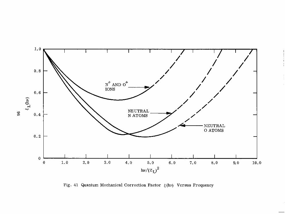
0.8
0.6
I I /
/ / / / / /
/ /
/ /
/ / /
NEUTRAL ’ /’ /
/ -NEUTRAL
0 ATOMS
I
/
/
/
2.0 3.0 4.0 5.0 6.0 7.0 8.0 9.0 10.0
hu/( ZL)2
Fig. 41 Quantum Mechanical Correction Factor <(hv) Versus Frequency

Appendix B
STREAM TUBE CHEMISTRY CALCULATION
The rate-governed production of species was calculated using a Lockheed numerical
computer code on a Univac 1107 digital computer. The computer code, itself, is a
version of the more or less standard stream-tube rate chemistry method. For
detailed description the reader is referred to J. G. Hall et al. (Ref. 28) one of sev-
eral references describing the method and application. A fundamental assumption
underlying this method is that the principle evolution of specie components takes
place in the direction of the streaming fluid motion (streamline directions) and that
the small transverse contributions (across streamlines) can be neglected in many
kinds of inviscid non-equilibrium flow processes.
The coupled array of differential species production processes is numerically inte-
grated along a streamline subject to a prescribed pressure or velocity distribution.
This distribution is obtained from a prior (equilibrium) flow calculation. The motion
of the fluid element is thus described by the designated distribution in conjunction with
the one dimensional stream-line momentum equation:
where x is the streamline coordinate. Hence, the motion of the fluid element (or,
in general, the position in space and time of the evolving chemical constituent species)
is governed by the results of an auxiliary calculation. This considerably simplifies
the code problem to one of forward integration of the coupled chemical rate processes
within a fluid element following a designated trajectory in space and time.
The specific version of the code used in the present, calculations is described in con-
siderable detail in Vinokur et al. (Ref. 29). Briefly an array of 10 component species
97

of rrairn (considered, initially, as an undisturbed binary mixture of 79 parts molecular
nitrogen to 21 parts molecular oxygen) is treated using 7 basic differential rate proc-
esses and 3 algebraic species conservation statements. In formulation the system
follows closely the work of G. Emanuel (Ref. 30). The 7 basic rate processes are
augmented by consideration of multiple third body collision partners of variable
efficiency. This consideration essentially increases the number of differential rate
processes to 20 (Ref. 29).
The state of the gas at any position is described by a simple equation of state appro-
priate for a multi-component mixture of ideal constituents,
P(x) = PWQX) 2 iii(X) i=l
along with an energy (enthalpy) relation,
ii(x) = f iii(X) [ - - CpiT(x) + eDi + eIi 1 i=l
L(x) = @total) - U(i)2
which completes the system along with the array of differential species production
processes written symbolically,
1 diii(x) CL(x) * - = ~
is9 dx
In the foregoing equations, p , p , and T are the stream pressure, density and kinetic
temperature, ni the ith constituent molar ratio, Cpi the specific heat capacity of
98

the ith constituent at constant pressure, eD and e1 i i the ith component dissocia-
tion and ionization energies, u the streaming velocity and Gsi the usual rate of pro-
duction term for the th i species. The barred designation indicates appropriate
non-dimensional form of the variables (Ref. 29). The gas itself is considered
instantaneously fully excited in rotational and vibrational degrees of freedom, equili-
brated to the translational mode.
Forward rate constants were adopted from the lists in J. G. Hall et al. (Ref. 28) and
M. H. Bortner (Ref. 31). Equilibrium constants were developed from the spectroscopic
data of Herzberg (Ref. 32), Moore (Ref. 19) and listed nergy states of Gilmore (Ref. 33).
Program output includes temperature, density, pressure, enthalpy, velocity and the
molar ratios for the 10 component species all as a function of streamline position.
The components considered for air are: 02, N2, NO, 0, N, NO+, N 2+’
O+, N+, and
free electrons.
99

REFERENCES
1. R. E. Meyerott, J. Sokoloff, and R. W. Nicholls, “Absorption Coefficients of Air, ”
Geophysical Research Paper 58, GRD-TN-60-277, Jul 1960
2. B. Kivel and K. Bailey, “Tables of Radiation From High Temperature Air, ”
AVCO Research Report 21, Dee 1957
3. B. H. Armstrong, S. Brush, H. Dewitt, R. R. Johnston, P. S. Kelley, and
0 . R. Platas, “Opacity of High-Temperature Air,” AFWL-TR 65-17, Air Force
Weapons Laboratory
4. M. C. Nardone, R. G. Breene, S. S. Zelden, and T. R. Riethof, “Radiance of
Species in High Temperature Air, ” GE-MSD Document R63SD23, Jun 1963
5. . . G E Hahne, “The Vacuum Ultraviolet Radiation From N+- and O+- Electron
Recombination in High-Temperature Air, ” NASA TN-D-2794, Ames Research
Center, Moffett Fieidki Calif. , Jun 1965 -.
6. . H Hoshizaki, “Equilibrium Total Radiation Measurements in Air at Super-
Orbital Entry Velocities, I’ Third Hypervelocity Techniques Symposium, Denver,
Mar 1964
7. R. M. Nerem and George H. Stickford, “Shock Layer Radiation During Hyper-
velocity Re-Entry, ” AIAA J. , 3, No. 6, loll- 1018 (1965)
8. D. M. Tellep and D K. Edwards, “Radiant Energy Transfer in Gaseous Flows,”
LMSD-288139, Lockheed Missiles & Space Company, Sunnyvale, Calif.,
January 1960
9. L. M. Biberman and G. E. Norman, Recombination Radiation and Brehmstrahlung
of a Plasma (Free-bound and Free-free Electron Transitions in a Field of Positive
Ions), Vol. 3, 221-245, 1963
100

10. A. Burgess and M. J. Seaton, “A General Formula for Calculation of Atomic
Photo-Ionization Cross Sections, ” Monthly Notices Roy. Astron. Sot. , 120, No. 2,
121-151 (1960)
11. L. M. Biberman, V. S. Vorobev, and G E. Norman, “Energy Emitted in Spectral
Lines by a Plasma at Equilibrium,” Optics and Spec. , l4, No. 3, 176-179 (1963)
12. V. S. Vorobev and G. E. Norman, “Energy Radiated in Spectral Lines by an
Equilibrium Plasma, II,” Optics and Spec., I7, No. 2 (1964)
13. L. H. Aller, Astrophysics, The Ronald Press Co., New York, 1963
14. G. M. Lawrence and B. D. Savage, “Radiative Lifetimes of UV Multiplets in
Boron, Carbon, and Nitrogen, If Phys. Rev., 141, No. 1 (1966)
15. B. M. Glennon, M. W. Smith, and W. L. Wiese, “Atomic Transition Probabilities,
H to Ne,” National Bureau of Standards, NSRDS-NBS4 (in print)
16. H. R. Griem, Plasma Spectroscopy, McGraw-Hill Book Co., New York, 1964
17. J. C. Stewart and K. D. Pyatt, “Theroetical Study of Optical Properties, ”
AFSWC-TR-61-71, Vol. I, Sep 1961
18. G. N. Plass, “Models for Spectral Band Absorption, ” 5. Opt. Sot. Am., 48,
No. 10, 690-703 (1958)
19. C. E. Moore, “Atomic Energy Levels, ” NBS Circular 467, Jun 1949
20. L. M. Biberman, et al., “Radiation Heating in Hypersonic Flow, ” Kosmich.
Issled . , 2, No. 3, 441-554 (1964) (trans. from the Russian)
21. N. H. Johannesen and H. Hoshizaki, “Effect of Radiation on Flow Properties
Behind Strong Shock Waves in Air, ” Nov 1962
22 . J. Wilson, “Ionization Rate of Air Behind High Speed Shock Waves, ” AVCO
Research Laboratory, Research Report 222, Ott 1965
23. J. D. Laird, and K. Heron, “Shock Tube Gas Dynamic Charts,” Part I: Equilibrium
Argon-Free Air From 3000 to 4O,OOO”K, AVCO RAD Technical Memorandum
RAD-TM-64-12, Apr 1964.
101

24. Rabinowicz, Jessey, and Bartsch, “Resistance Thermometer for Heat Transfer
in a Shock Tube, *I GALCIT Hypersonic Research Project, Memorandum 32,
Jul 1956
25 R J Vidal, “Model Instrumentation Techniques for Heat Transfer and Force . . .
Measurements in a Hypersonic Shock Tunnel, If CAL Report AD-917-A-1, Feb 1956
2 6. A. G. Gaydon, and I. R . Hur le, The Shock Tube in High-Temperature Chemical
Physics, New York, Reinhold Pub. Corp., 1963
27. P. V. Marrone and R. A. Hartuman, “The Performance of Thin-Film Thermome-
ters in Partially Ionized Shock-Tube Flows, I’ CAL Report AD-1118-A-5, AFOSR
TN 59-1046, Nov 1959
28. J. G. Hall, A. Q. Eschenroeder, P. V. Marrone, “Inviscid Hypersonic Air
Flows With Coupled Non-Equilibrium Processes, ‘I J. Aero. Sci. , 3, (1962)
29. M. Vinokur, W. E. Nicolet, A. C. Buckingham, H. Hoshizaki, “Project Fire
Flow Field Prediction and Analysis, ‘I LMSC M-12-65-1, Lockheed Missile &
Space Company, 1965
30 G Emanuel, “Problems Underlying the Numerical Integration of the Chemical . .
and Vibrational Rate Equations in Non-Equilibrium Flow, I’ AEDC TDR 63-82, 1963
31. M. H. Bortner, “Chemical Kinetics in a Re-entry Flow Field, I’ General Electric
Research Report R63SD63, 1963
32. G. Herzberg, Molecular Spectra and Molecular Structure, I, Spectra of Diatomic
Molecules, 20 ed D. Van Nostrand, Princeton, N. J., 1950 ,’
33. F. R. Gilmore, Rand Technical Report, RM 3748 - PR, 1963
102 NASA-Langley, 1966 c@335

“The aeronautical and space activities of the United States shall be conducted so as to contribute . . . to the expansion of hsman knowl- edge of phenomena in the atmosphere and space. The Administra/io, shall provide for the widest prac/icabie and appropriate dissemination of information concerning its activities and the resnh thereof.”
-NATIONAL AERONAUTICS AND SPACE ACT OF 1958
NASA SCIENTIFIC AND TECHNICAL PUBLICATIONS
TECHNICAL REPORTS: Scientific and technical information cbnsidered important, complete, and a lasting contribution to existing knowledge.
TECHNICAL NOTES: Information less broad in scope but nevertheless of importance as a contribution to existing knowledge.
c TECHNICAL MEMORANDUMS: Information receiving limited distri- butioh because of preliminary data, security classification, or other reasons.
CONTRACTOR REPORTS: Technical information generated in con- nection with a NASA contract or grant and released under NASA auspices.
TECHNICAL TRANSLATIONS: Information published in a foreign language considered to merit NASA distribution in English.
TECHNICAL. REPRINTS: Information derived from NASA activities and initially published in the form of journal articles.
SPECIAL PUBLICATIONS: Information derived from or of value to NASA activities but not necessarily reporting the results .of individual NASA-programmed scientific efforts. Publications include conference proceedings, monographs, data compilations, handbooks, sourcebooks, and special bibliographies.
Details on the availability of these publications may be obtained from:
SClENTlFlC AND TECHNICAL INFORMATION DIVISION
NATIONAL AERONAUTICS AND SPACE ADMINISTRATION
Washington, D.C. PO546