radiation from a moving charge - australian national …geoff/hea/2_radiating_charges.pdf= c 0e2n...

Radiation from a Moving Charge

1 The Lienard-Weichert radiation field

For details on this theory see the accompanying background notes onelectromagnetic theory (EM_theory.pdf)

Much of the theory in this chapter can be applied to many cases ofradiating charges. Its main use will be in the application to synchro-tron radiation.

Other reading: Rybicki & Lightman, Radiative Processes in Astro-physics, on which the following development is mainly, but not en-tirely, based. In particular, the emissivity in the Stokes parameters isnot dealt with in R&L.

High Energy Astrophysics: Radiating charges © Geoffrey V. Bicknell

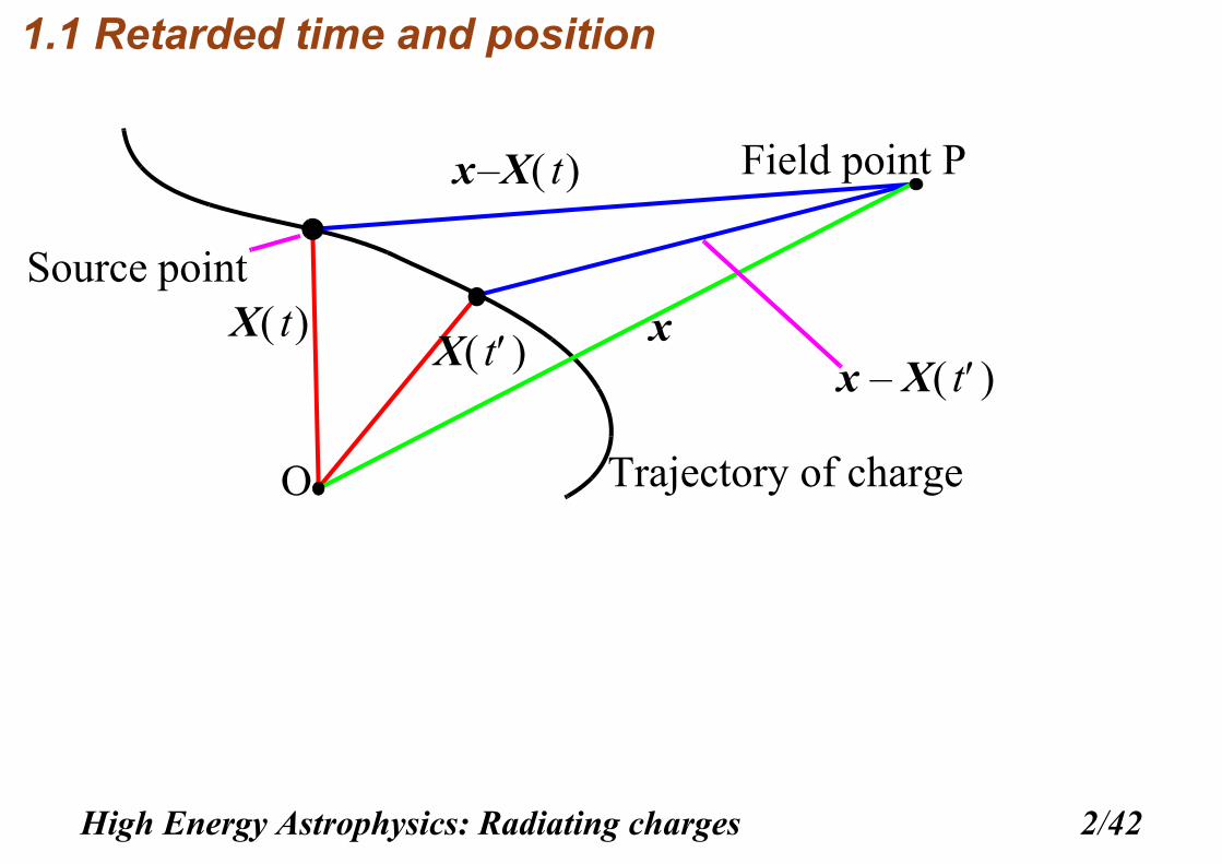
1.1 Retarded time and position

O

xX t

X t

x X t –

x X t –

Field point P

Trajectory of charge

Source point

High Energy Astrophysics: Radiating charges 2/42

In the above diagram:

(1)

O Arbitrary coordinate origin=

P Field point=

t time=

t Retarded time=

x Position vector of field point=

X t Position vector of moving charge (source point)=

X t Position vector of moving charge at retarded time=


Retarded time and retarded position vector

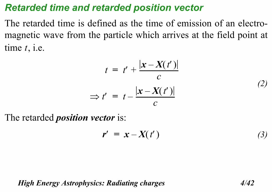
The retarded time is defined as the time of emission of an electro-magnetic wave from the particle which arrives at the field point attime , i.e.

(2)

The retarded position vector is:

(3)

t

t t x X t –c

------------------------+=

t tx X t –

c------------------------–=

r x X t –=


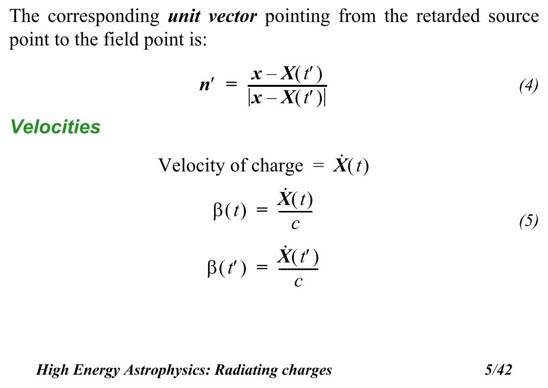
The corresponding unit vector pointing from the retarded sourcepoint to the field point is:

(4)

Velocities

(5)

n x X t –x X t –------------------------=

Velocity of charge X· t =

t X· t c

----------=

t X· t c

------------=


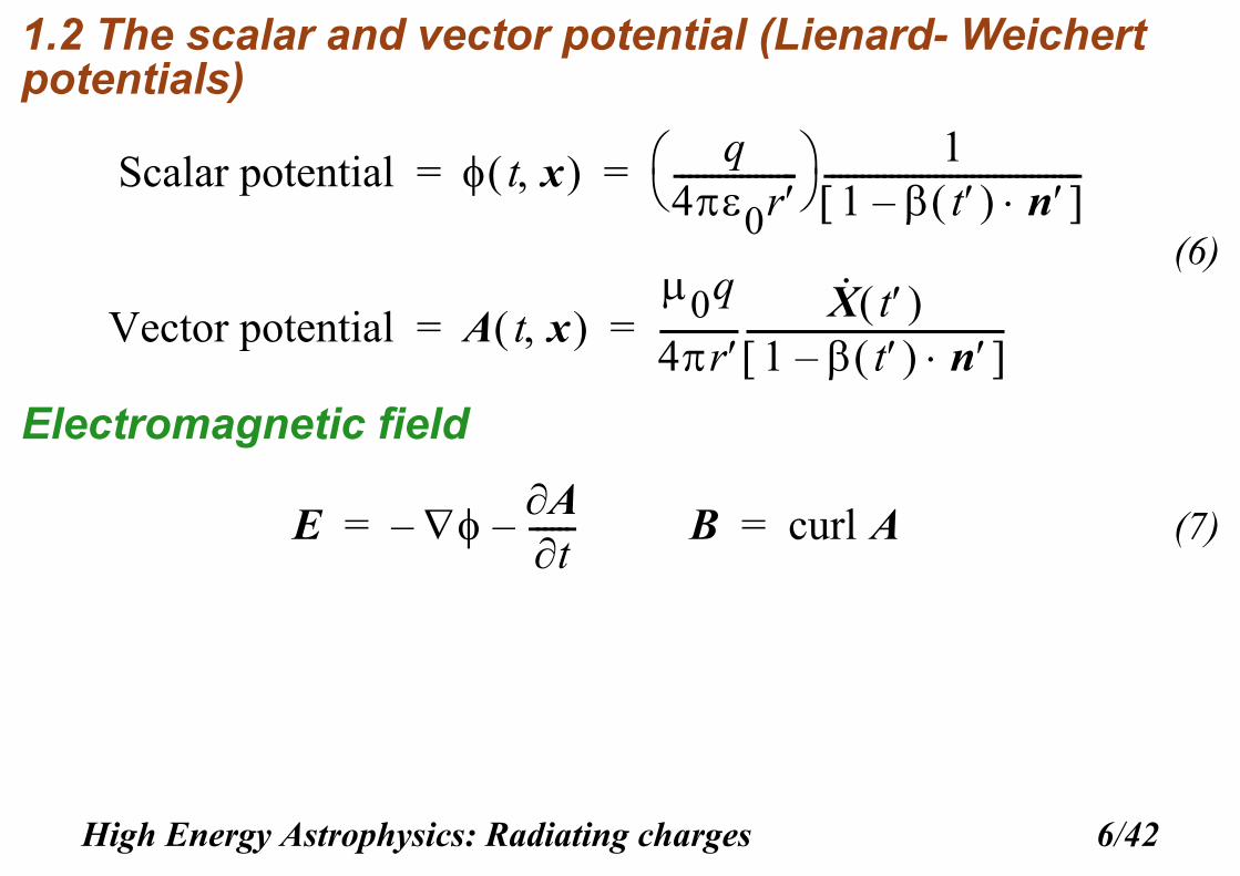
1.2 The scalar and vector potential (Lienard- Weichert potentials)

(6)

Electromagnetic field

(7)

Scalar potential t x q40r----------------- 1

1 t n– -----------------------------------= =

Vector potential A t x 0q

4r-----------

X· t 1 t n–

-----------------------------------= =

E –At

------–= B curl A=


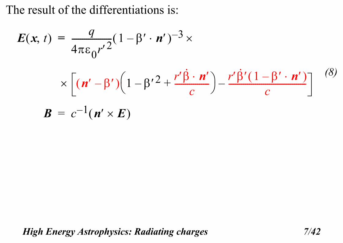
The result of the differentiations is:

(8)

E x t q

40r2-------------------- 1 n– 3– =

n – 1 2–r· n

c-----------------+

r· 1 n– c

--------------------------------------–

B c 1– n E =


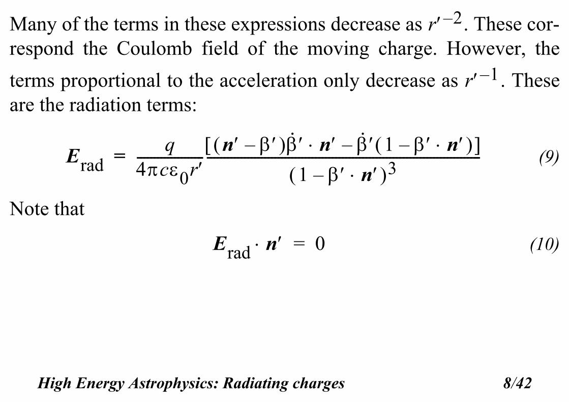
Many of the terms in these expressions decrease as . These cor-respond the Coulomb field of the moving charge. However, the

terms proportional to the acceleration only decrease as . Theseare the radiation terms:

(9)

Note that

(10)

r 2–

r 1–

Eradq

4c0r--------------------

n – · n · 1 n– – 1 n– 3

---------------------------------------------------------------------------------=

Erad n 0=


Poynting flux

The Poynting flux of the Lienard-Weichert electromagnetic field isgiven by:

(11)

This can be understood in terms of equal amounts of electric and

magnetic energy density ( ) moving at the speed of light in

the direction of . This is a very important expression when itcomes to calculating the spectrum of radiation emitted by an accel-erating charge.

SE B0

--------------E n E

c0------------------------------ c0 E2n E n E– = = =

c0E2n= for the radiation component

0 2 E2

n


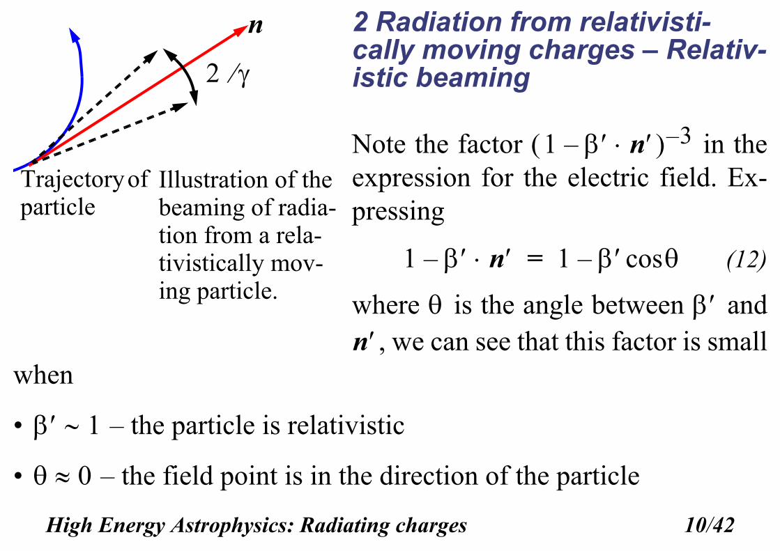
2 Radiation from relativisti-cally moving charges – Relativ-istic beaming

Note the factor in theexpression for the electric field. Ex-pressing

(12)

where is the angle between and, we can see that this factor is small

when

• – the particle is relativistic

• – the field point is in the direction of the particle

Trajectory of particle

2

n

Illustration of the beaming of radia-tion from a rela-tivistically mov-ing particle.

1 n– 3–

1 n– 1 cos–=

n

1

0


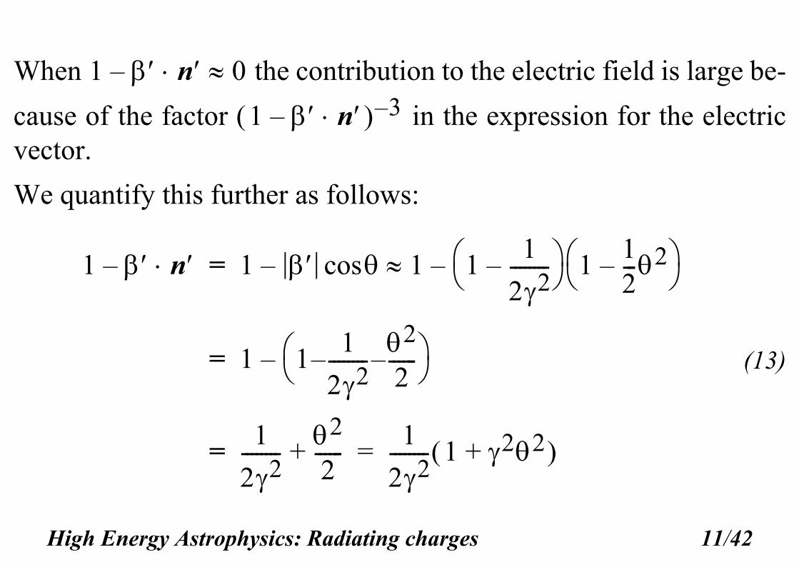
When the contribution to the electric field is large be-

cause of the factor in the expression for the electricvector.

We quantify this further as follows:

(13)

1 n– 0

1 n– 3–

1 n– 1 1 11

22--------–

112---2–

–cos–=

1 11

22--------

2

2------––

–=

1

22--------

2

2------+=

1

22-------- 1 22+ =


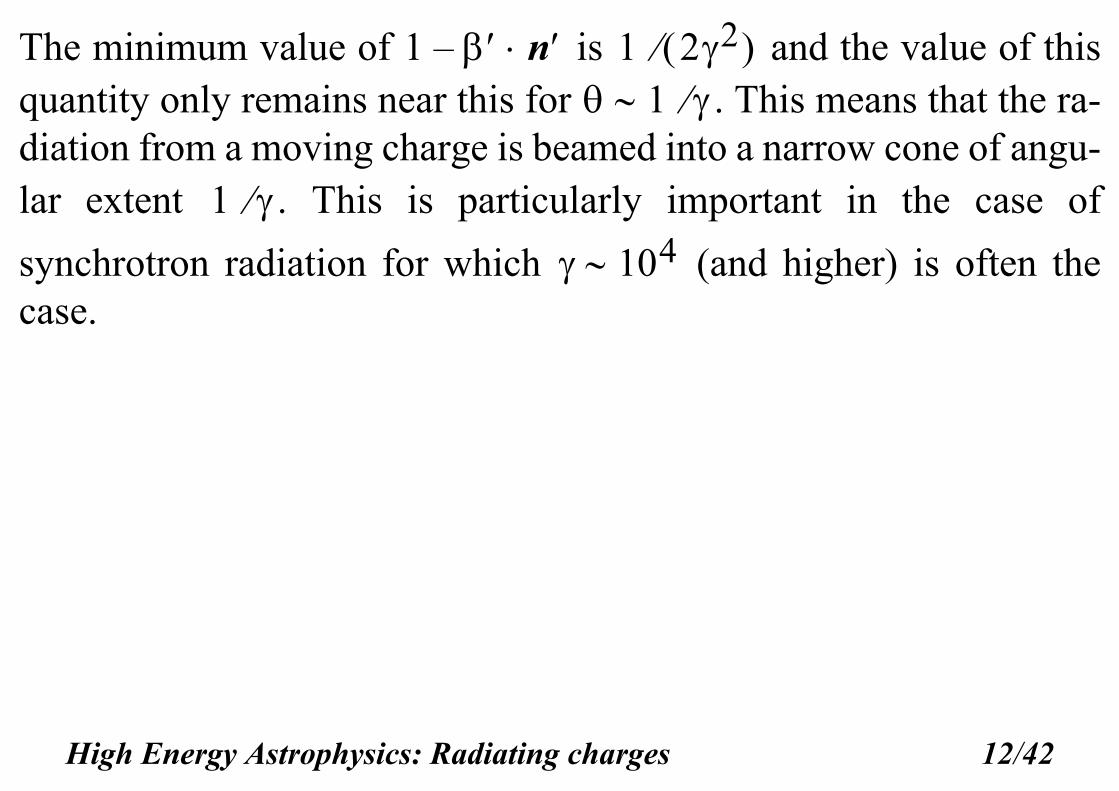
The minimum value of is and the value of thisquantity only remains near this for . This means that the ra-diation from a moving charge is beamed into a narrow cone of angu-lar extent . This is particularly important in the case of

synchrotron radiation for which (and higher) is often thecase.

1 n– 1 22 1

1

104


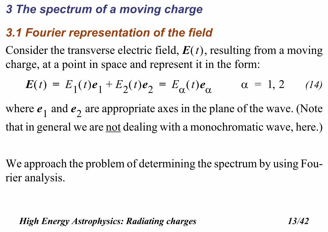
3 The spectrum of a moving charge

3.1 Fourier representation of the field

Consider the transverse electric field, , resulting from a movingcharge, at a point in space and represent it in the form:

(14)

where and are appropriate axes in the plane of the wave. (Note

that in general we are not dealing with a monochromatic wave, here.)

We approach the problem of determining the spectrum by using Fou-rier analysis.

E t

E t E1 t e1 E2 t e2+ E t e= = 1 2=

e1 e2


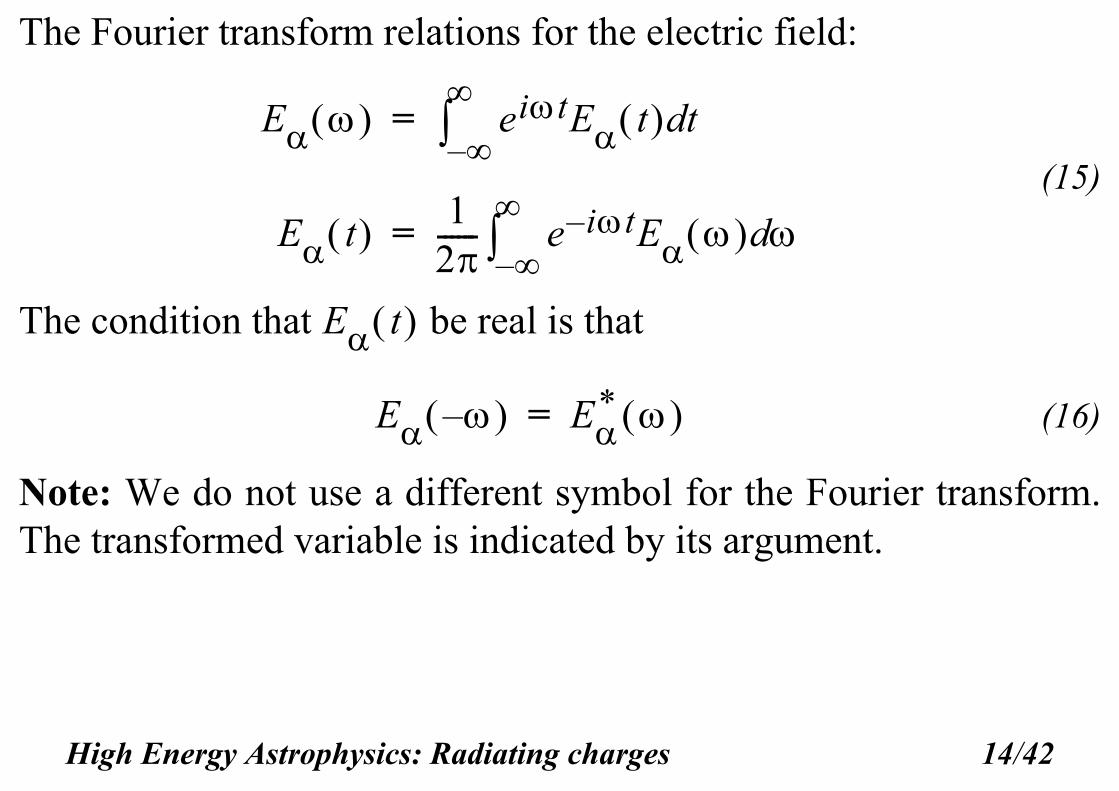
The Fourier transform relations for the electric field:

(15)

The condition that be real is that

(16)

Note: We do not use a different symbol for the Fourier transform.The transformed variable is indicated by its argument.

E eitE t td–

=

E t 12------ e it– E d

–

=

E t

E – E* =


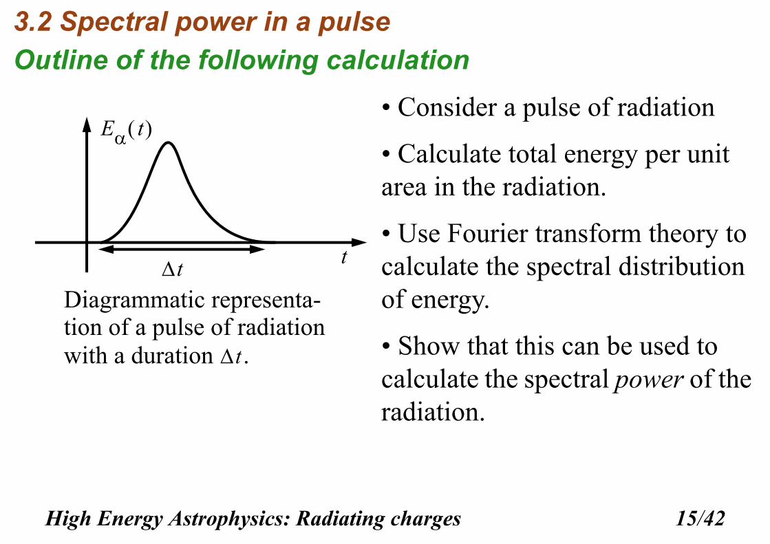
3.2 Spectral power in a pulse

Outline of the following calculation

• Consider a pulse of radiation

• Calculate total energy per unit area in the radiation.

• Use Fourier transform theory to calculate the spectral distribution of energy.

• Show that this can be used to calculate the spectral power of the radiation.

E t

t

Diagrammatic representa-tion of a pulse of radiation with a duration .t

t


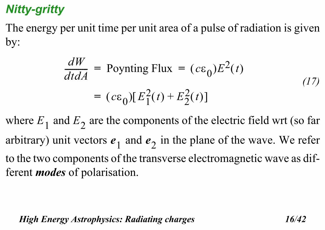
Nitty-gritty

The energy per unit time per unit area of a pulse of radiation is givenby:

(17)

where and are the components of the electric field wrt (so far

arbitrary) unit vectors and in the plane of the wave. We refer

to the two components of the transverse electromagnetic wave as dif-ferent modes of polarisation.

dWdtdA------------ Poynting Flux c0 E2 t = =

c0 E12 t E2

2 t + =

E1 E2

e1 e2


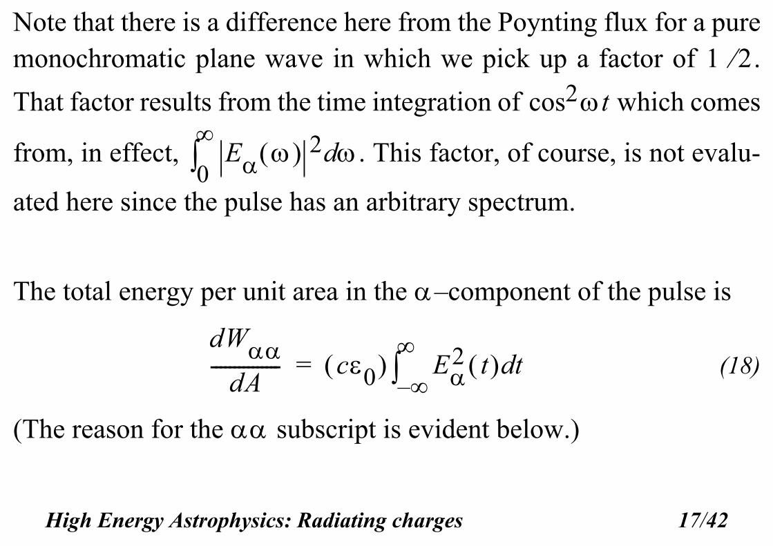
Note that there is a difference here from the Poynting flux for a puremonochromatic plane wave in which we pick up a factor of .

That factor results from the time integration of which comes

from, in effect, . This factor, of course, is not evalu-

ated here since the pulse has an arbitrary spectrum.

The total energy per unit area in the –component of the pulse is

(18)

(The reason for the subscript is evident below.)

1 2

tcos2

E 2 d0

dWdA

--------------- c0 E2 t td

–

=


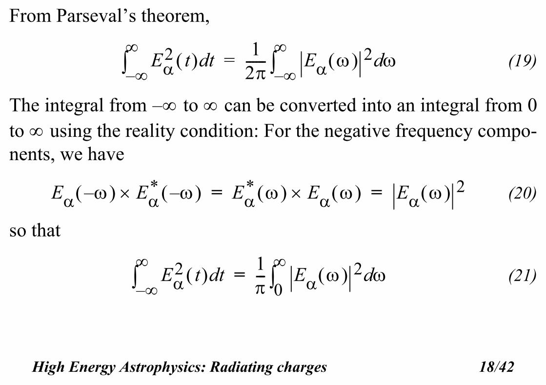
From Parseval’s theorem,

(19)

The integral from to can be converted into an integral from 0to using the reality condition: For the negative frequency compo-nents, we have

(20)

so that

(21)

E2 t td

–

12------ E 2 d

–

=

–

E – E* – E

* E E 2= =

E2 t td

–

1--- E 2 d

0

=


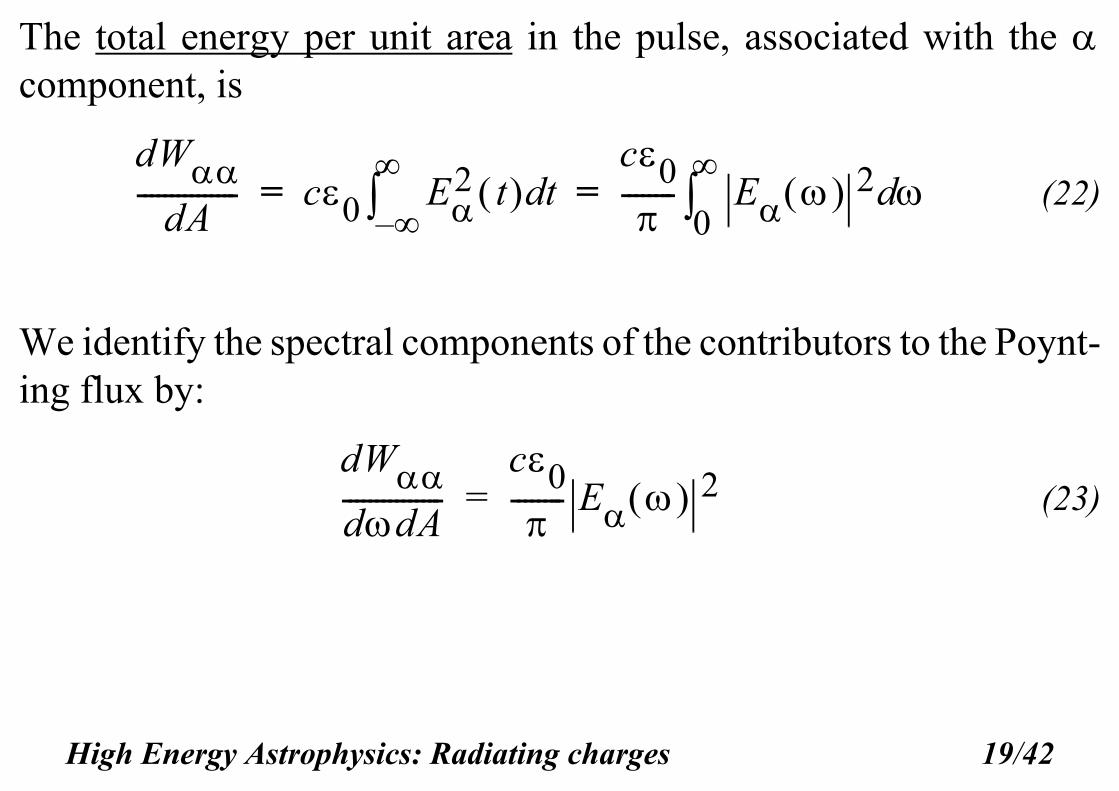
The total energy per unit area in the pulse, associated with the component, is

(22)

We identify the spectral components of the contributors to the Poynt-ing flux by:

(23)

dWdA

--------------- c0 E2 t td

–

c0

-------- E 2 d0

= =

dWddA---------------

c0

-------- E 2=


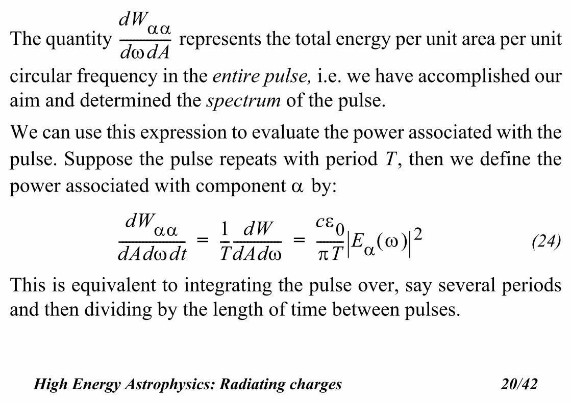
The quantity represents the total energy per unit area per unit

circular frequency in the entire pulse, i.e. we have accomplished ouraim and determined the spectrum of the pulse.

We can use this expression to evaluate the power associated with thepulse. Suppose the pulse repeats with period , then we define thepower associated with component by:

(24)

This is equivalent to integrating the pulse over, say several periodsand then dividing by the length of time between pulses.

dWddA---------------

T

dWdAddt--------------------

1T---

dWdAd--------------

c0T-------- E 2= =


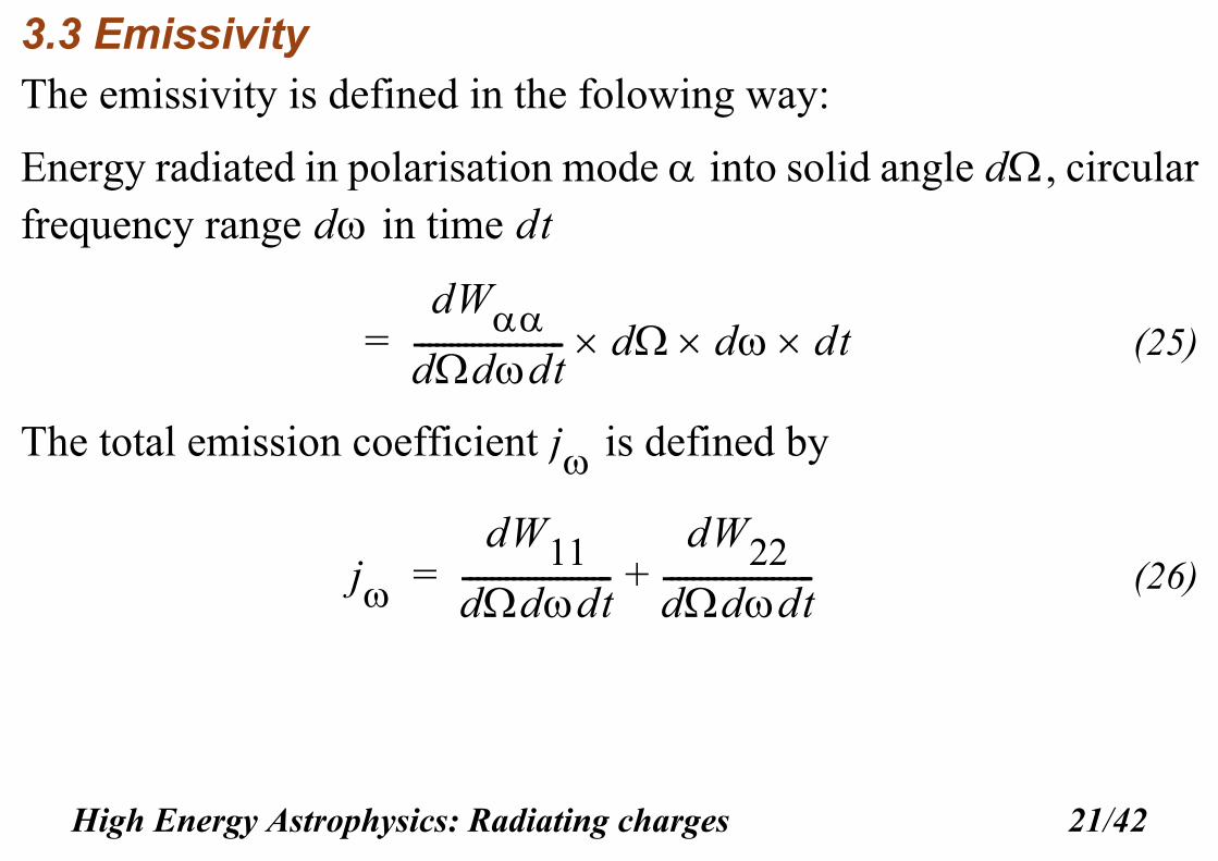
3.3 EmissivityThe emissivity is defined in the folowing way:

Energy radiated in polarisation mode into solid angle , circularfrequency range in time

(25)

The total emission coefficient is defined by

(26)

dd dt

dWdddt--------------------- d d dt=

j

j

dW11dddt---------------------

dW22dddt---------------------+=


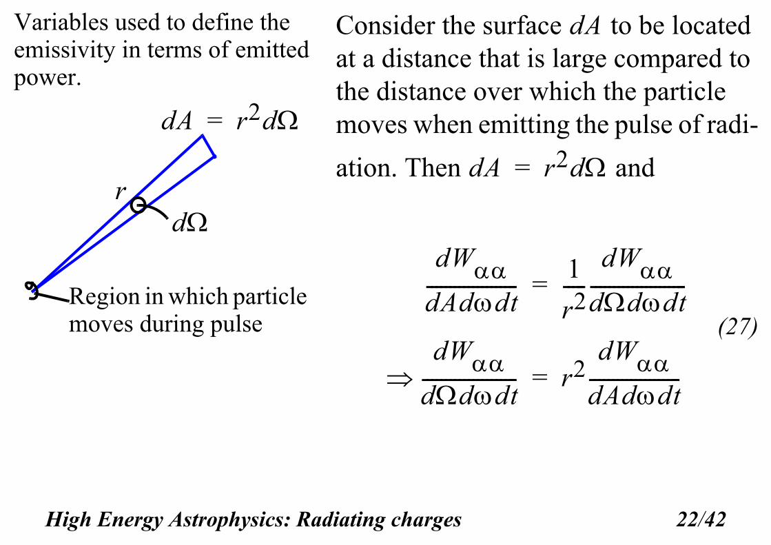
Consider the surface to be located at a distance that is large compared to the distance over which the particle moves when emitting the pulse of radi-

ation. Then and

(27)

Variables used to define the emissivity in terms of emitted power.

Region in which particle moves during pulse

dA r2d=

dr

dA

dA r2d=

dWdAddt--------------------

1

r2-----

dWdddt---------------------=

dWdddt--------------------- r2

dWdAddt--------------------=


Emissivity corresponding to the component of pulse.

(28)

3.4 Independence of radiusNote that

(29)

e

dWdddt---------------------

c0r2

T-------------- E 2=

c0r2

T--------------= E E

* (Summation not implied)

dWdddt--------------------- r2 E 2


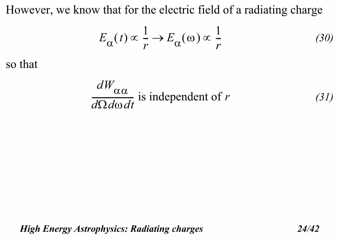
However, we know that for the electric field of a radiating charge

(30)

so that

(31)

E t 1r--- E 1

r---

dWdddt--------------------- is independent of r


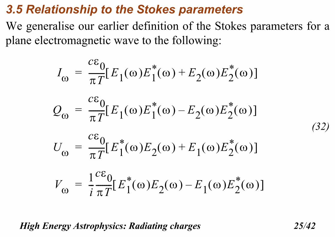
3.5 Relationship to the Stokes parametersWe generalise our earlier definition of the Stokes parameters for aplane electromagnetic wave to the following:

(32)

I

c0T-------- E1 E1

* E2 E2* + =

Q

c0T-------- E1 E1

* E2 E2* – =

U

c0T-------- E1

* E2 E1 E2* + =

V1i---

c0T-------- E1

* E2 E1 E2* – =


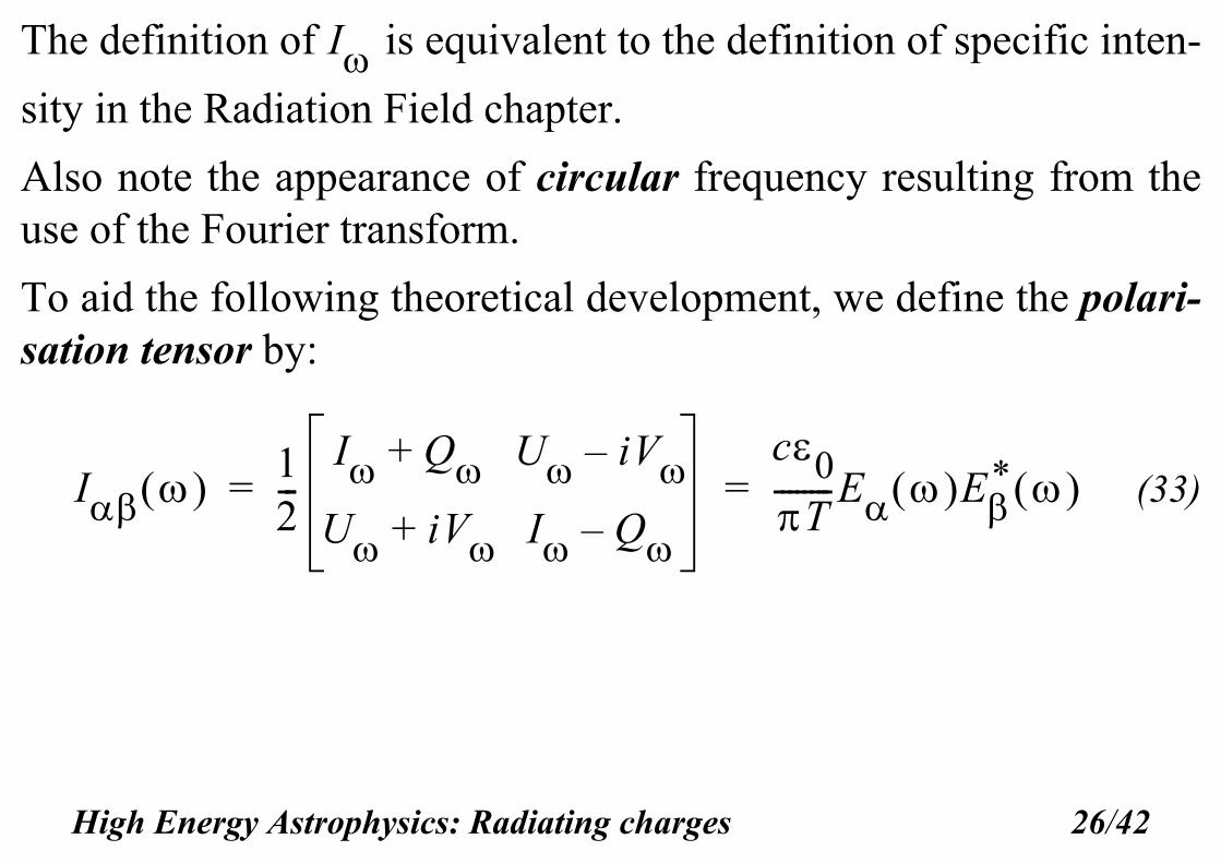
The definition of is equivalent to the definition of specific inten-

sity in the Radiation Field chapter.

Also note the appearance of circular frequency resulting from theuse of the Fourier transform.

To aid the following theoretical development, we define the polari-sation tensor by:

(33)

I

I 12---

I Q+ U iV–

U iV+ I Q–

c0T--------E E

* = =


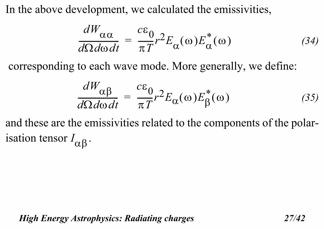
In the above development, we calculated the emissivities,

(34)

corresponding to each wave mode. More generally, we define:

(35)

and these are the emissivities related to the components of the polar-isation tensor .

dWdddt---------------------

c0T--------r2E E

* =

dWdddt---------------------

c0T--------r2E E

* =

I


In general, therefore, we have

(36)

dW11dddt--------------------- Emissivity for

12--- I Q+


12--- I Q–


12--- U iV–

dW21dddt---------------------

dW12*

dddt--------------------- Emissivity for

12--- U iV+ =


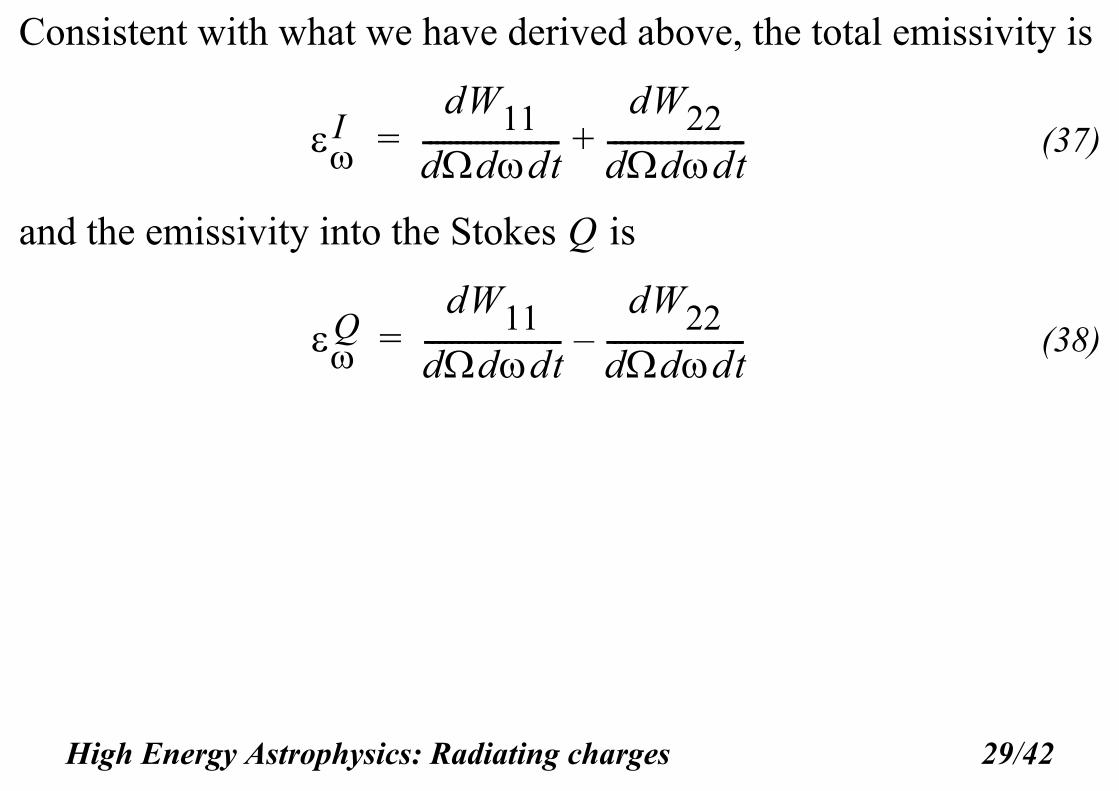
Consistent with what we have derived above, the total emissivity is

(37)

and the emissivity into the Stokes is

(38)

I

dW11dddt---------------------

dW22dddt---------------------+=

Q

Q

dW11dddt---------------------

dW22dddt---------------------–=


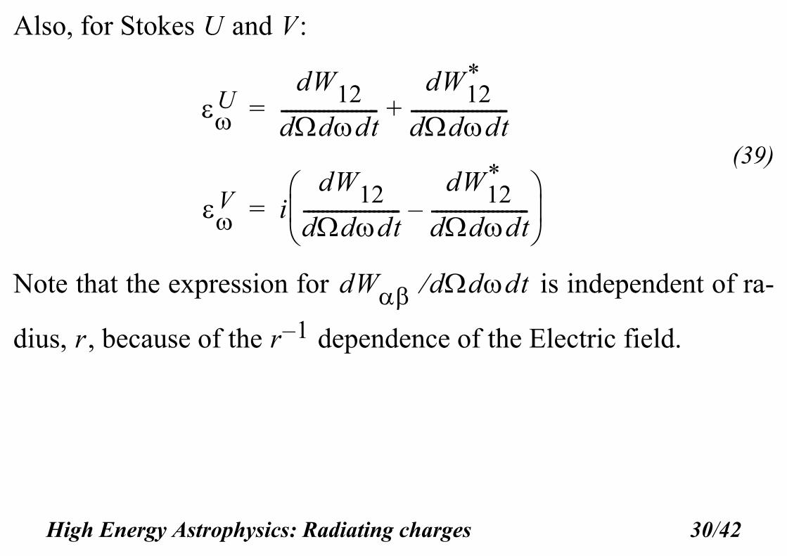
Also, for Stokes and :

(39)

Note that the expression for is independent of ra-

dius, , because of the dependence of the Electric field.

U V

U

dW12dddt---------------------

dW12*

dddt---------------------+=

V i

dW12dddt---------------------

dW12*

dddt---------------------–

=

dW dddt

r r 1–


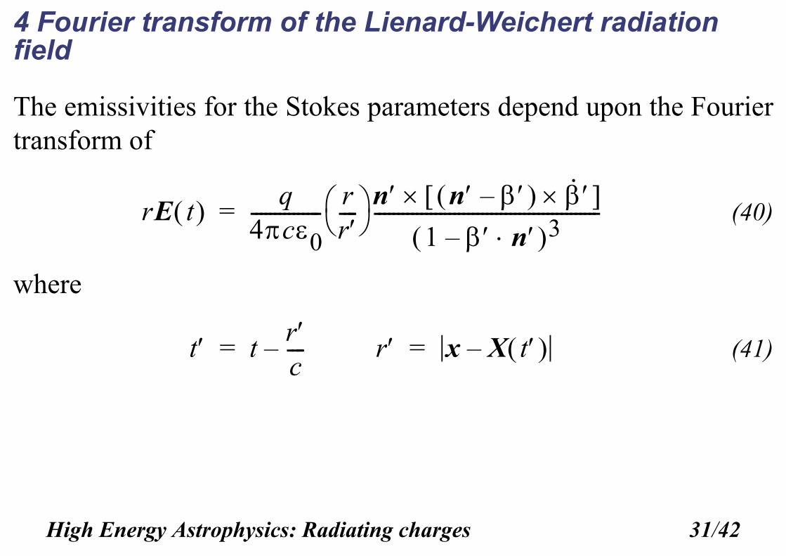
4 Fourier transform of the Lienard-Weichert radiation field

The emissivities for the Stokes parameters depend upon the Fouriertransform of

(40)

where

(41)

rE t q4c0---------------

rr---- n n – ·

1 n– 3------------------------------------------------=

t trc----–= r x X t –=


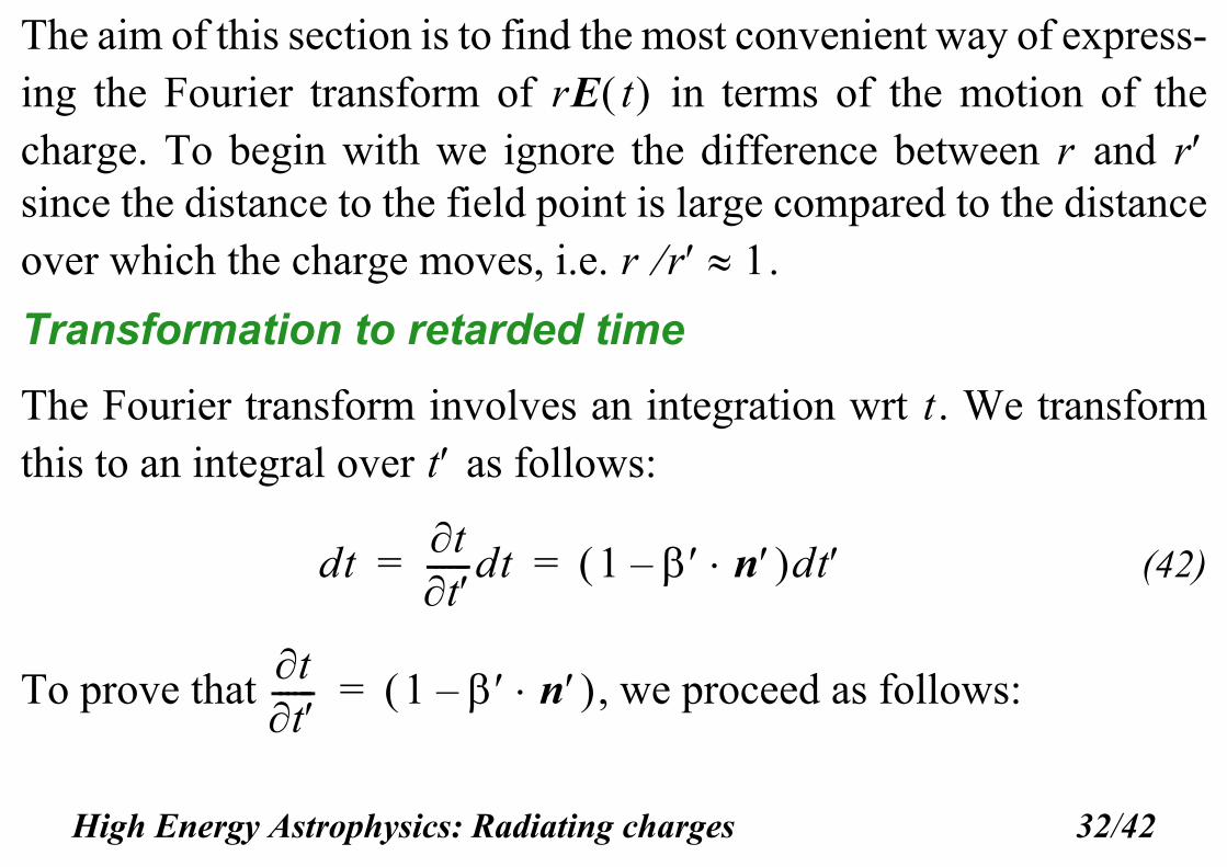
The aim of this section is to find the most convenient way of express-ing the Fourier transform of in terms of the motion of thecharge. To begin with we ignore the difference between and since the distance to the field point is large compared to the distanceover which the charge moves, i.e. .

Transformation to retarded time

The Fourier transform involves an integration wrt . We transformthis to an integral over as follows:

(42)

To prove that , we proceed as follows:

rE t r r

r r 1

tt

dttt

------dt 1 n– dt= =

tt

------ 1 n– =


The relationship between field point time and source point time (re-tarded time) is given by:

(43)

Differentiate wrt :

(44)

Now,

t

t t x X t –c

------------------------+=

t

tt

11c---

t

x X t –+=

t

x X t –t

xi Xi t – xi Xi t – 1 2/=


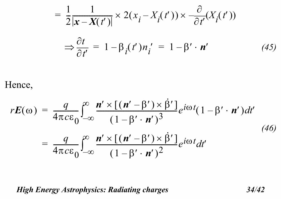
(45)

Hence,

(46)

12---

1x X t –------------------------ 2 xi Xi t –

t

– Xi t ( )=

tt 1 i t ni– 1 n–= =

rE q4c0---------------

n n – · 1 n– 3

------------------------------------------------eit 1 n– td–

=

q4c0---------------

n n – · 1 n– 2

------------------------------------------------eit td–

=


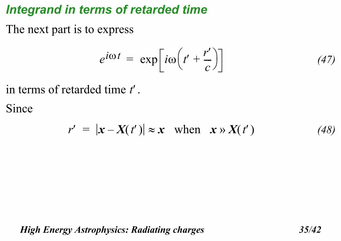
Integrand in terms of retarded time

The next part is to express

(47)

in terms of retarded time .

Since

(48)

eit i t rc----+

exp=

t

r x X t – x when x X t »=


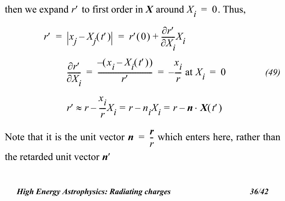
then we expand to first order in around . Thus,

(49)

Note that it is the unit vector which enters here, rather than

the retarded unit vector

r X Xi 0=

r xj Xj t – r 0 rXi

--------Xi+= =

rXi

--------xi Xi t – –

r--------------------------------

xir---- at Xi– 0= = =

r rxir----Xi– r niXi– r n X t –= =

nrr--=

n


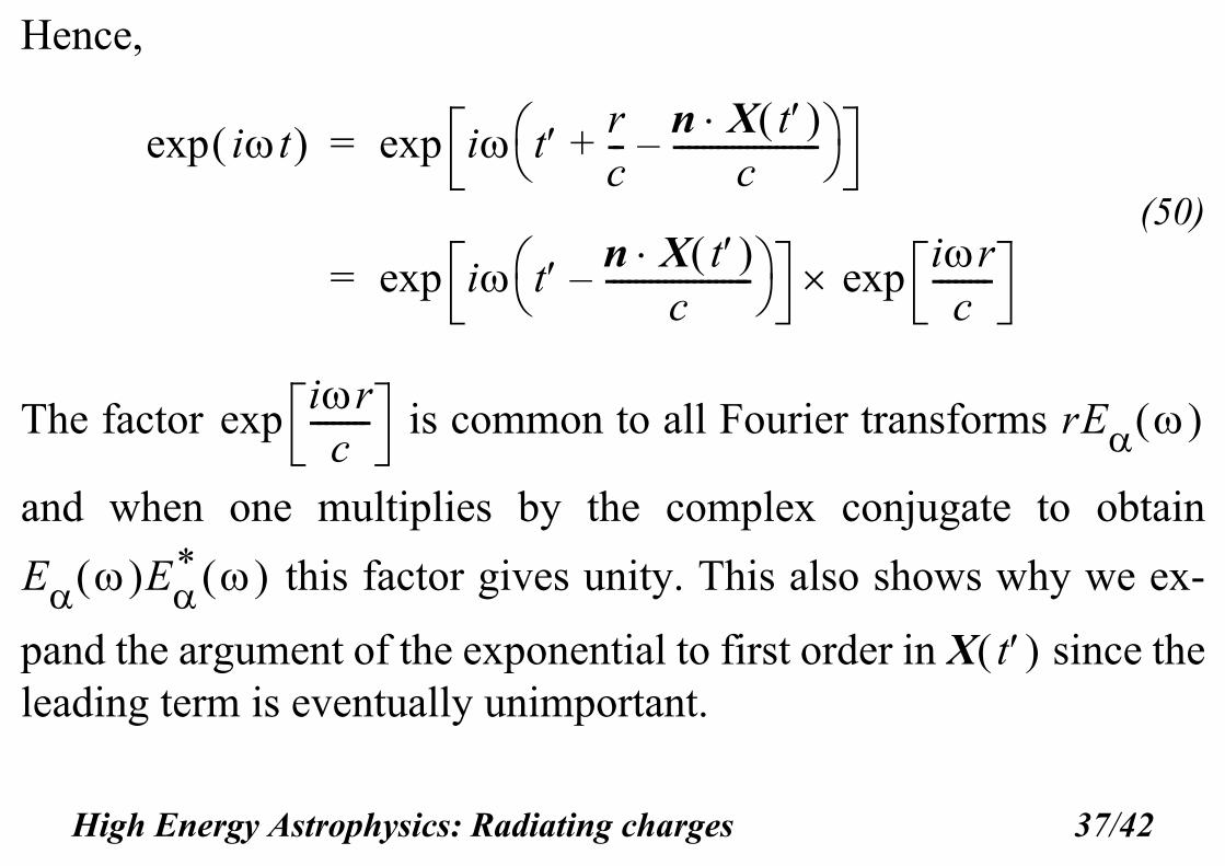
Hence,

(50)

The factor is common to all Fourier transforms

and when one multiplies by the complex conjugate to obtain

this factor gives unity. This also shows why we ex-

pand the argument of the exponential to first order in since theleading term is eventually unimportant.

it exp i t rc--

n X t c

--------------------–+ exp=

i t n X t c

--------------------– ir

c--------expexp=

irc

--------exp rE

E E*

X t


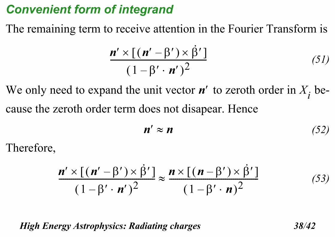
Convenient form of integrand

The remaining term to receive attention in the Fourier Transform is

(51)

We only need to expand the unit vector to zeroth order in be-

cause the zeroth order term does not disapear. Hence

(52)

Therefore,

(53)

n n – · 1 n– 2

------------------------------------------------

n Xi

n n

n n – · 1 n– 2

------------------------------------------------n n – ·

1 n– 2---------------------------------------------


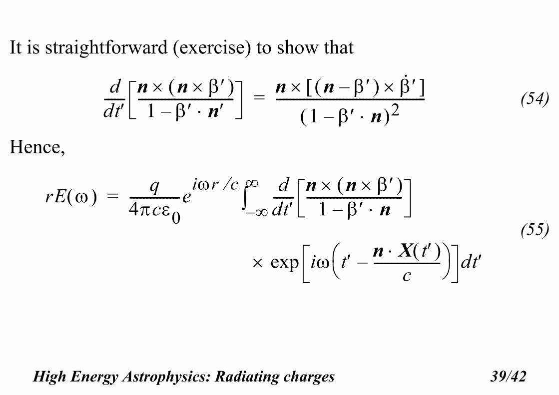
It is straightforward (exercise) to show that

(54)

Hence,

(55)

ddt------

n n 1 n–

-----------------------------n n – ·

1 n– 2---------------------------------------------=

rE q4c0---------------e

ir c ddt------

n n 1 n–

-----------------------------–

=

i t n X t c

--------------------– exp dt


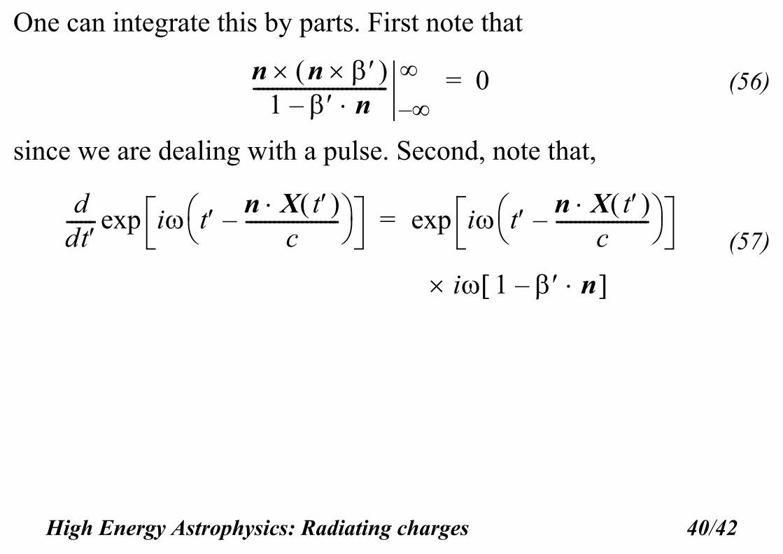
One can integrate this by parts. First note that

(56)

since we are dealing with a pulse. Second, note that,

(57)

n n 1 n–

-----------------------------–

0=

ddt------ i t n X t

c--------------------–

exp i t n X t c

--------------------– exp=

i 1 n–


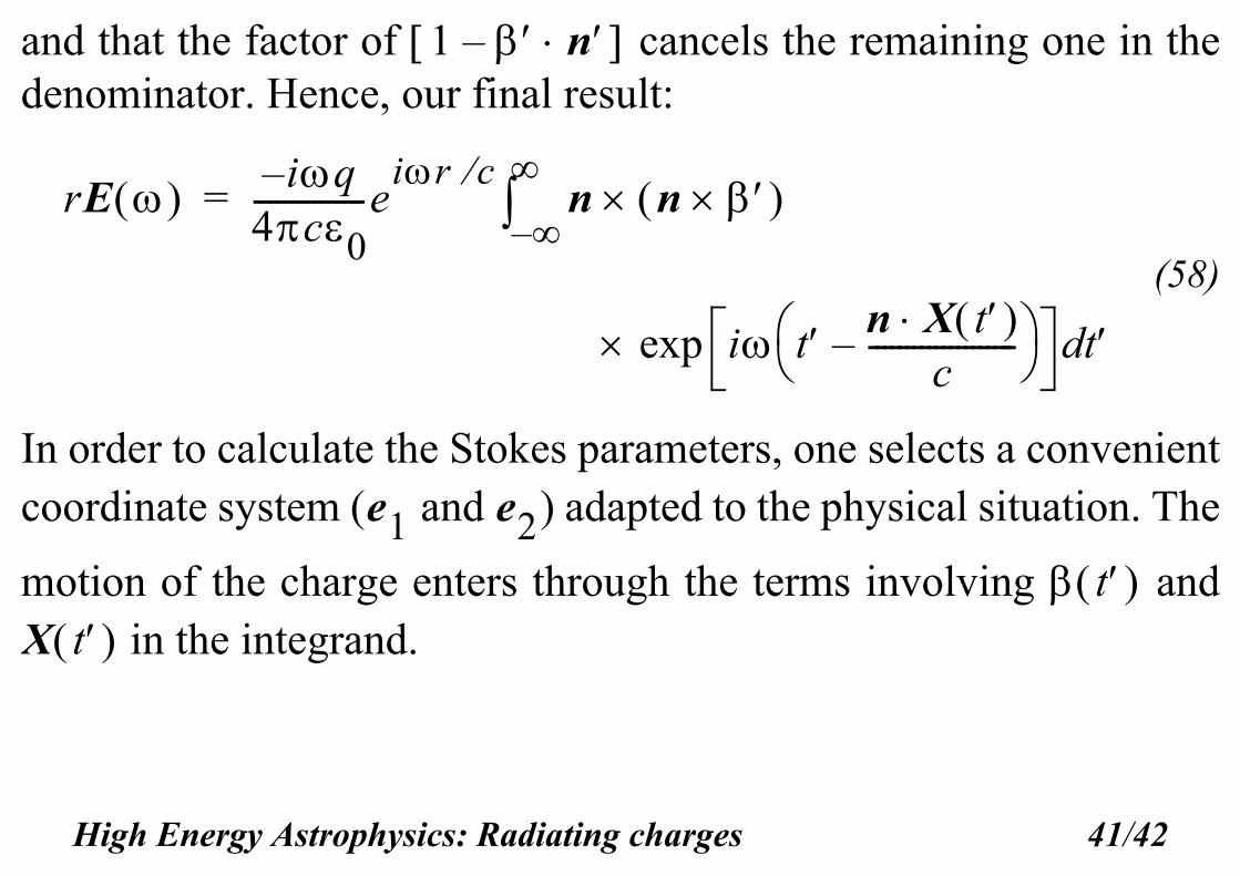
and that the factor of cancels the remaining one in thedenominator. Hence, our final result:

(58)

In order to calculate the Stokes parameters, one selects a convenientcoordinate system ( and ) adapted to the physical situation. The

motion of the charge enters through the terms involving and in the integrand.

1 n–

rE iq–4c0---------------e

ir cn n

–

=

i t n X t c

--------------------– exp td

e1 e2

t X t


Remark on relativistic beaming

The feature associated with radiation from a relativistic particle,namely that the radiation is very strongly peaked in the direction ofmotion, shows up in the previous form of this integral via the factor

. This dependence is not evident here. However, whenwe proceed to evaluate the integral in specific cases, this dependenceresurfaces.

1 n– 3–


radiation from a moving charge - australian national …geoff/hea/2_radiating_charges.pdf= c 0e2n...

Documents