radiation heat transfer in a particulate medium using a
TRANSCRIPT

Louisiana State UniversityLSU Digital Commons
LSU Master's Theses Graduate School
2015
Radiation Heat Transfer In A Particulate MediumUsing A Ray Tracing MethodManish B. PatilLouisiana State University and Agricultural and Mechanical College, [email protected]
Follow this and additional works at: https://digitalcommons.lsu.edu/gradschool_theses
Part of the Mechanical Engineering Commons
This Thesis is brought to you for free and open access by the Graduate School at LSU Digital Commons. It has been accepted for inclusion in LSUMaster's Theses by an authorized graduate school editor of LSU Digital Commons. For more information, please contact [email protected].
Recommended CitationPatil, Manish B., "Radiation Heat Transfer In A Particulate Medium Using A Ray Tracing Method" (2015). LSU Master's Theses. 3516.https://digitalcommons.lsu.edu/gradschool_theses/3516

ii
RADIATION HEAT TRANSFER IN A PARTICULATE
MEDIUM USING A RAY TRACING METHOD
A Thesis
Submitted to the Graduate Faculty of the
Louisiana State University and
Agricultural and Mechanical college
in partial fulfillment of
requirements for the degree of
Master of Science in Mechanical Engineering
in
The Department of Mechanical and Industrial Engineering
by
Manish B. Patil
Bachelor of Mechanical Engineering, University of Mumbai, 2009
May 2016

1
ACKNOWLEDGEMENTS
My education at LSU would not have been possible without the support of Dr. Shengmin
Guo, my guide, mentor and my major advisor. He gave me confidence and support
during my course works and other endeavors at LSU. I would like to thank him whole
heartedly for not only guiding me through my projects, but also for helping me improve
as a person. I also would like to express my special thanks to Dr. Muhammad Wahab and
Dr. Ram Devireddy for being a part of my committee, and providing a valuable feedback
on my work and career as well.
I want to thanks my labmates and friends Susheel Singh, Pranaya Pokharel and Mohana
Durga Prasad for their support. I also thank my friends and relatives, here and back in
India who supported me through all my ups and downs in my life; and for keeping me
motivated all the time.
This study is supported by Louisiana Board of Regents and LaSPACE grant LEQSF-
EPS(2014)-RAP -12 and NSF-Consortium for innovation in manufacturing and materials
(CIMM) program (grant number # OIA-1541079 ). I would like to thank them for their
generous support.
Finally, I dedicate this work to my Aai, Baba and my brother Dhanu for being with me
all the time with their never ending love and prayers.
ii

2
TABLE OF CONTENTS
ACKNOWLEDGEMENTS ................................................................................................ ii
LIST OF TABLES .............................................................................................................. v
LIST OF FIGURES ........................................................................................................... vi
ABSTRACT ........................................................................................................................ x
CHAPTER 1: INTRODUCTION ....................................................................................... 1
1.1 Radiation Heat Transfer in Particulate Medium .................................................... 1
1.2 Parameters of Radiative Transport in a Particulate medium : ................................ 2
1.3 Methods to evaluate scattering phase functions in particulate medium: ................ 7
1.4 Roseland Diffusion Approximation: ...................................................................... 8
1.5 Introduction to the integro-differential equation in interacting medium. ............... 9
CHAPTER 2: RATIONALE AND OBJECTIVE ............................................................ 11
2.1 Rationale: .............................................................................................................. 11
2.2 Objectives: ............................................................................................................. 13
2.3 Theoretical framework for the problem: ............................................................... 14
CHAPTER 3: LITERATURE REVIEW .......................................................................... 21
3.1 Background on radiative transport in packed bed systems : ................................. 21
3.2 Background on selective laser melting process: .................................................. 28
CHAPTER 4: BED GENERATION METHOD AND MONTE CARLO PROCEDURE
........................................................................................................................................... 30
4.1 Simulation of packed beds: ................................................................................... 30
4.2 Types of packed beds: ............................................................................................ 32
4.3 Procedure used to create the random packing: ...................................................... 34
4.4 The schematic diagram for the randomly packed bed program: ........................... 36
4.5 Porosity of the packed beds ................................................................................... 37
4.6 Monte Carlo Method : ........................................................................................... 40
4.7 Properties of metallic powder bed while using the Mote Carlo simulation: ......... 43
4.8 Laser Power Sources: ........................................................................................... 50
iii

3
CHAPTER 5: RESULTS .................................................................................................. 52
5.1 Analysis of Radiative Transport in Thick Particulate Beds - ................................ 57
5.2 Analysis of Radiative Transport in Thin particulate layers : ............................... 71
CHAPTER 6: CONCLUSION ......................................................................................... 90
REFERENCES ................................................................................................................. 91
APPENDIX ....................................................................................................................... 94
VITA ............................................................................................................................... 126
iv

4
LIST OF TABLES
Table 1: Input parameters for validation case (Thick bed) ............................................... 57
Table 2: Input parameters for simple cubic bed ................................................................ 61
Table 3: Input parameters for Rhombohedral packing ..................................................... 64
Table 4: Input parameters for the comparison of two flux method, present monte carlo
and unit cell type monte carlo method .............................................................................. 75
v

5
LIST OF FIGURES
Figure 1: (a) Interaction of photon and particle (b) scattering, transmission and
absorption. (Modest, 2003) ................................................................................................. 3
Figure 2: Types of scattering .............................................................................................. 5
Figure 3: Specular and Diffuse Reflection (Modest,2003) ................................................. 8
Figure 4 : Schematic diagram for absorbing, emitting and scattering medium .................. 9
Figure 5: Laser beam shining over a porous bed .............................................................. 14
Figure 6: Forward and backward scatted components with collimated laser source and
reflection from bottom surface.......................................................................................... 19
Figure 7 : Experimental setup for radiation heat transfer through packed bed systems
(Chen and Churchill,1987)................................................................................................ 23
Figure 8: Comparison of previous models and experimental data for the transmittance
through packed bed systems (Tien et al.,1987)................................................................. 24
Figure 9. Independent versus Dependent scattering regimes using the particle size
parameter and the volume fraction. (Tien et al.,1987). ..................................................... 25
Figure 10: Square or simple cubic packing of spherical particles .................................... 32
Figure 11:Rhombohedral Packing of spherical Particles. ................................................. 33
Figure 12: Random Packing of spherical particles in cube............................................... 33
Figure 13: Different packed beds arrangements generated using random packing
algorithm. .......................................................................................................................... 35
Figure 14: Schematic diagram for random packing algorithm ......................................... 36
Figure 15 : Porosity calculation in four simple cubic and rhombohedral spheres ............ 37
Figure 16 : 0.5 x 0.5 mm simple cubic bed with 0.1mm particle size .............................. 37
Figure 17 : Porosity as a function of bed height in a simple cubic packing configuration38
Figure 18: 0.54 x 0.54 mm Rhombohedrally packed bed with 0.1 mm particle size ..... 38
Figure 19 Porosity as a bed height in rhombohedral packing ........................................... 39
vi

6
Figure 20 : 0.54 x 0.52 x0.54 mm randomly packed bed with 0.7 to 1 mm particle size . 40
Figure 21: Porosity as a function of bed height in random packing ................................ 40
Figure 22: Spiral Input function for laser source .............................................................. 42
Figure 23: Specular Reflection ......................................................................................... 43
Figure 24: Scattering phase function for diffuse reflection generated using Henyey-
Greenstein phase function (at g = -0.7) using random numbers. ...................................... 44
Figure 25: Coordinate system for packed bed .................................................................. 47
Figure 26: Schematic diagram for Monte Carlo Method. ................................................ 49
Figure 27 Collimated and Diffuse source ......................................................................... 50
Figure 28: Gaussian source over a packed bed ................................................................. 50
Figure 29: Gaussian power source for laser beam (100 W) , 0.4 mm diameter ............... 51
Figure 30: Uniformly distributed source (100W), Diameter: 0.4 mm ............................. 51
Figure 31: Transmission of radiation in simple cubic packing ........................................ 52
Figure 32: 2d Simulation for diffuse reflection with (~ 40 photons) ................................ 53
Figure 33: 2d Simulation for specular reflection with (~ 40 photons) ............................. 53
Figure 34 : 2d simulation for Isotropic scattering in packed spherical bed using
Henyey-Greenstein Phase Function (g = 0) ...................................................................... 55
Figure 35:2d Simulation for backward scattering in packed, spherical beds using
Henyey-Greenstein Phase Function (g = -0.7) ................................................................. 55
Figure 36: 2d Simulation for Forward scattering in packed beds using Henyey-Greenstein
Phase Function (g = + 0.7) ................................................................................................ 56
Figure 37 Comparison with the experimental results ....................................................... 58
Figure 38 Radiative heat Transfer in simple cubic arrangement ...................................... 62
Figure 39: Transmission in Rhombohedral packed bed ................................................... 65
Figure 40 Transmission in Different bed configurations (Specular Reflection) ............... 66
Figure 41:Energy Absorbed by the beds with different types of packing arrangements .. 67
vii

7
Figure 42 Substrate Reflection simulation ....................................................................... 67
Figure 43 : (a) Radiation Energy Flux and (b) Absorption Profile in randomly packed
bed at different porosities ( Specular Reflection) ............................................................. 68
Figure 44 : Effect of Porosity in randomly packed bed (Specular reflection) .................. 69
Figure 45 : Optimum porosity for maximum radiative transport ..................................... 70
Figure 46 Absorbing and reflecting substrates ............................................................... 72
Figure 47 Specular and diffuse reflection in thin layers with perfectly absorbing substrate
........................................................................................................................................... 73
Figure 48 Unit cell type of Monte Carlo ........................................................................... 74
Figure 49 Simple Cubic Packing : Present Monte-Carlo, Two flux method and unit cell
Monte Carlo over perfectly reflecting substrate. .............................................................. 76
Figure 50 Rhombohedral packing : Present Monte-Carlo, Two flux method and unit cell
Monte Carlo over perfectly reflecting substrate. .............................................................. 77
Figure 51 Small Particulate thick layer: Present Monte-Carlo, Two flux method and unit
cell Monte Carlo over perfectly reflecting substrate ......................................................... 78
Figure 52: Reflecting Substrate ........................................................................................ 79
Figure 53: Effect of different bottom boundary conditions in thin layers ........................ 80
Figure 54: Comparison between Absorbing boundary and reflecting boundary .............. 81
Figure 55: Effect of substrate reflection on energy absorbed by the bed ......................... 82
Figure 56 : 2d simulation showing the angle of incidence on a packed bed (~ 40 photons)
........................................................................................................................................... 83
Figure 57: Energy Absorbed by the bed at different angle of incidence .......................... 84
Figure 58: Total Energy absorbed by the bed against angle of incidence ....................... 84
Figure 59 Effect of Angle of Incidence ............................................................................ 85
Figure 60: Energy absorbed by the substrate against angle of incidence (Diffuse
reflection) .......................................................................................................................... 86
Figure 61 Complete energy distribution for the bed ......................................................... 87
viii

8
Figure 62 : Effect of variation in power inputs for a thin layer ........................................ 88
Figure 63:Gaussian source and Uniform source ............................................................... 89
ix

9
ABSTRACT
In the present work, a complete 3D simulation of ray tracing model is developed for
studying the radiation heat transfer, associated with laser based additive manufacturing,
in both thick and thin particulate beds by using the Monte Carlo method. Additional
program is developed for creating different types of packing structures such as simple
cubic, rhombohydral and random packing. The scattering mechanisms in the particulate
beds for large opaque spheres are evaluated using the specular and diffuse reflection
methods. Further, a novel approach has been added to the model to include isotropic,
forward and backward scattering mechanisms for a medium which consists of particles
with very small size parameters. Henyey Greenstein phase function is used to evaluate
the scattering for extremely small, particulate porous beds.
For thick layers, a thorough study has been carried out on the effect of porosity, bed
thickness, power inputs and different bed configurations. Whereas for thin layers, the
substrate conditions are studied in detail. Then they are analyzed for variation in energy
absorbed. The effects of reflective and absorbing boundary conditions are also studied.
For the incoming beam both uniform and Gaussian distributions with different angles of
incidence has been simulated. The effect of various size parameters on the radiative
transport has also been compared for both thick and thin layers. Finally, for thin layers,
the model is compared with the two flux method and the unit cell Monte-Carlo method.
x

1
CHAPTER 1: INTRODUCTION
1.1 Radiation Heat Transfer in Particulate Medium
Radiative heat transfer in a particulate medium is a classic problem that has been studied
for several decades. When an incoming wave of photons travel through the interacting
medium made up of small particles, it affects the direction, intensity, and the wavelength
of the incident wave (Modest, 2003). In this process, some photons are absorbed,
reflected, transmitted and sometimes emitted by the particles. These types of media are
defined as an absorbing, emitting and scattering media. The radiative transport in such
mediums is significantly affected by the optical and physical properties of the particles in
the medium. However, the optical properties are also subjected to change with change in
wavelength of incoming beam. The optical properties that affects the radiation transport
are refractive indices (m), absorptance, reflectivity, transmittance and scattering, whereas
the physical properties of particle are its shape, size parameter (x), surface roughness,
orientation, arrangement, volume density and opacity. It can be observed that, some of
these mediums have dominant absorption properties, some of them show very high
scattering behavior, and some others have almost no scattering effect. The most common
examples of such mediums are porous beds of metallic and nonmetallic substances,
oceans, human skin, planetary atmospheres with gases and dust particles etc. (Modest,
2003).
The physics of radiation transport can be effectively explained by the movement of
photons in a medium. The photons that come out from the particle after the interaction
are known as scattered photons. In other words, when the electromagnetic waves

2
encounters discontinuity in the refractive index, it is known as scattering (Larkin et. al.,
1959). Scattering can be a result of reflection, refraction, and diffraction as shown in
Figure 1 (a). If the photon moves in opposite direction to the incoming beam then it is
known as backward scattering and if it moves in same direction, it is known as forward
scattering. In diffraction, photon never comes in actual contact with the particle but its
direction of propagation is affected by the presence of the particle where as in refraction
photon travels through the particle, loses its energy and comes out of the particle in some
different direction (Howell et. al, 2010). As soon as a photon enters in a medium, the
change in the direction of the photon can be seen. This change is caused by the refractive
index of the medium. Generally speaking higher the refractive index, higher loss of
energy in travelling medium. It can be observed that the metals have quite high refractive
index compared with gases (Modest, 2003).
1.2. Parameters of Radiative Transport in a Particulate medium :
1.2.1 Particles in the medium
The radiation heat transfer in the particulate medium takes place on the basis of type of
transparency of the particle. The particles are classified as opaque, transparent or
semitransparent materials. The opaque particle is defined as a medium which is thick
enough so that the electromagnetic waves cannot penetrate through it. The surface of the
opaque particle can only reflect the radiative energy completely or partially. On the other
hand, the ideal transparent particle can easily transmit the wave through its body. In these
particles the change in direction of the wave depends solely upon the index of refraction
of the medium. It also has very high transmissivity and thus energy can travel to a
substantial distance in the medium. A semitransparent particle behaves in between

3
transparent and opaque particle. A particle is considered as semitransparent when the
electromagnetic wave can penetrate the particle till some appreciable distance. In these
particles, the depth of penetration also depends on the wavelength of the radiation. For
example, some small wavelengths are barely able to penetrate through the liquid glass.
Therefore, the liquid glass is not considered semitransparent for such wavelengths
(Modest, 2003).
Figure 1: (a) Interaction of photon and particle (b) scattering, transmission and
absorption. (Modest, 2003)
1.2.2 Types of Scatterings
The mechanism of radiation heat transport also significantly depends on the scattering
characteristics of the medium. These characteristics can further be classified as single or
multiple scattering, elastic or inelastic scattering and dependent or independent scattering
( Tien et. al.,1987).
a) Single and multiple scattering :
When a single photon is scattered by a particle then the scattering is known as single
scattering, whereas in multiple scattering, a gross effect of the large number of photons is

4
considered. Due to the randomness in the behavior of a single photon in the single
scattering, it is very difficult to determine the exact path followed by the photon.
Therefore the existence of the photon at particular location is defined by the probability
distribution function, whereas in multiple scattering, the combined effect of photonic
behavior is taken in to account, and the path followed by the photon is given in form of
statistical mean so that randomness can be averaged out.
b) Elastic and inelastic scatterings :
The elastic scattering is defined as, a process when the original wavelength of incoming
light remains unchanged after photon-particle interaction. The kinetic energy of incoming
wave is conserved in elastic scattering process. Whereas in inelastic scattering, the
wavelength and the energy of scattered radiation differs from the incoming radiation.
Hence, the kinetic energy of incoming wave is not conserved in inelastic scattering which
also makes the radiation heat transfer analysis less complex. The inelastic scattering is
also known as a Raman scattering effect. It is mentioned by Modest et, al., (2003) that
Raman scattering effect is very small from radiation heat transfer point of view so
inelastic scattering can be neglected. In the present work the scattering process in
assumed elastic.
c) Dependent and Independent Scattering :
The scattering in particulate medium is classified in dependent and independent
scattering regimes depending on the presence of neighboring particles. Dependent
scattering takes place when a scattered photon is affected by its neighboring particles.
Whereas, in independent scattering, the particles are sufficiently far away from each other

5
so that the proximity of the neighboring particle doesn't affect the interaction. Dependent
scattering is dominant in fluidized and packed beds, microsphere insulations, soot layers,
fuel pallets of nuclear reactor, packed-sphere and heat generators, whereas the examples
of independent scattering are fogs and clouds, pulverized coals, soots particles in flame,
paints and pigments etc. (Tien et. al.,1987).
1.2.3 Particle Size:
The most important physical properties of a particle are its size parameter and refractive
index. The size parameter (x) for the spherical particle is given by and complex
refractive index (m) is given by n+ ik where d is a diameter of the particle. The real part
n is the ratio of particle refractive index to the medium and an imaginary part k is the
extinction coefficient of complex refractive index of the particle. The refractive index for
dielectric materials is very small , but for metals it is quite high. (Tien et. al.,
1987).
Figure 2: Types of scattering
The limits of different size parameters (x) and extinction coefficient (k) helps to decide
the type of scattering theory to be used in the analysis. For very small particles, when
, Rayleigh scattering gives accurate results. Whereas for the larger particles

6
, geometric optics theory is suitable. Mie scattering theory is used for all size
parameters which also includes medium size particle, where the geometric optics is not
applicable. For large spheres , the extinction paradox shows that a large amount
of energy is extinct due to diffraction by the particle. The projected area for a large
particle ( d2) for absorption and reflection is almost doubled than the exposed surface
area. Hence, diffraction plays a dominant role when the particle size increases. This
results in the dominance of scattering in forward direction. So, for a large sphere,
Babinet's principle shows that almost all the energy is scattered forward within a narrow
cone ( , as shown in Figure 2 (c). Hence, the diffraction
from a large particle is either neglected or considered as transmission in heat transfer
applications. However, when large particles (both metals and dielectrics) are opaque,
transmission is not possible, and the ray which refracts towards a particle is absorbed by
the particle and if there is a forward scattering in opaque particle, it is only due to the
refraction. Therefore the refraction index of the material is also considered while
evaluating the size parameter for opaque spheres. Additional assumption ) is
taken into account for a large and opaque particle scattering (Modest, 2003).
For metals if x > 10 and k is significantly large then the particle is considered as
a large particle;
For dielectrics if x > 10000 and k is fairly small then the particle is considered
as a large particle. (Modest, 2003).

7
1.3. Methods to evaluate scattering phase functions in particulate medium:
1.3.1 Small and Medium Particle Size (Mie scattering) :
Mie scattering theory is usually used for all particle size parameters, however, the large
calculations make the analysis complex for large particles. In order to find the scattering
for particles using Mie scattering theory, it’s necessary to figure out various efficiency
factors. They are, absorption efficiency factor ( ), Scattering efficiency
factor ( ) and extinction efficiency factor ( ).
Also, . Where, is absorption cross section of the particle,
is the scattering cross section and stand for the extinction cross section of the
particle. The Mie theory shows that, for the large opaque particle extinction efficiency
approaches to 2 as the size parameter (x) increases. Present work deals with large opaque
particulate bed. In that case, the size parameter is significantly large so secular and
diffused reflections mechanism from the large particles are useful in current work.
1.3.2 Large Particle Size (Specular and Diffuse Reflection):
The scattering from the large opaque sphere is treated as either specular reflection or a
diffuse reflection. In specular reflection, the energy is scattered from the given single
point on the spherical surface whereas it for diffuse reflection the part of surface area of
the sphere is taken into account.
In the specular reflection the scattering phase function is given by the following
formula,
Where , is a scattering angle, is a hemispherical
reflectance or a fraction energy reflected by the particle and Scattering efficiency in a
specular reflection is . In a diffuse reflecting sphere, the phase function is
8
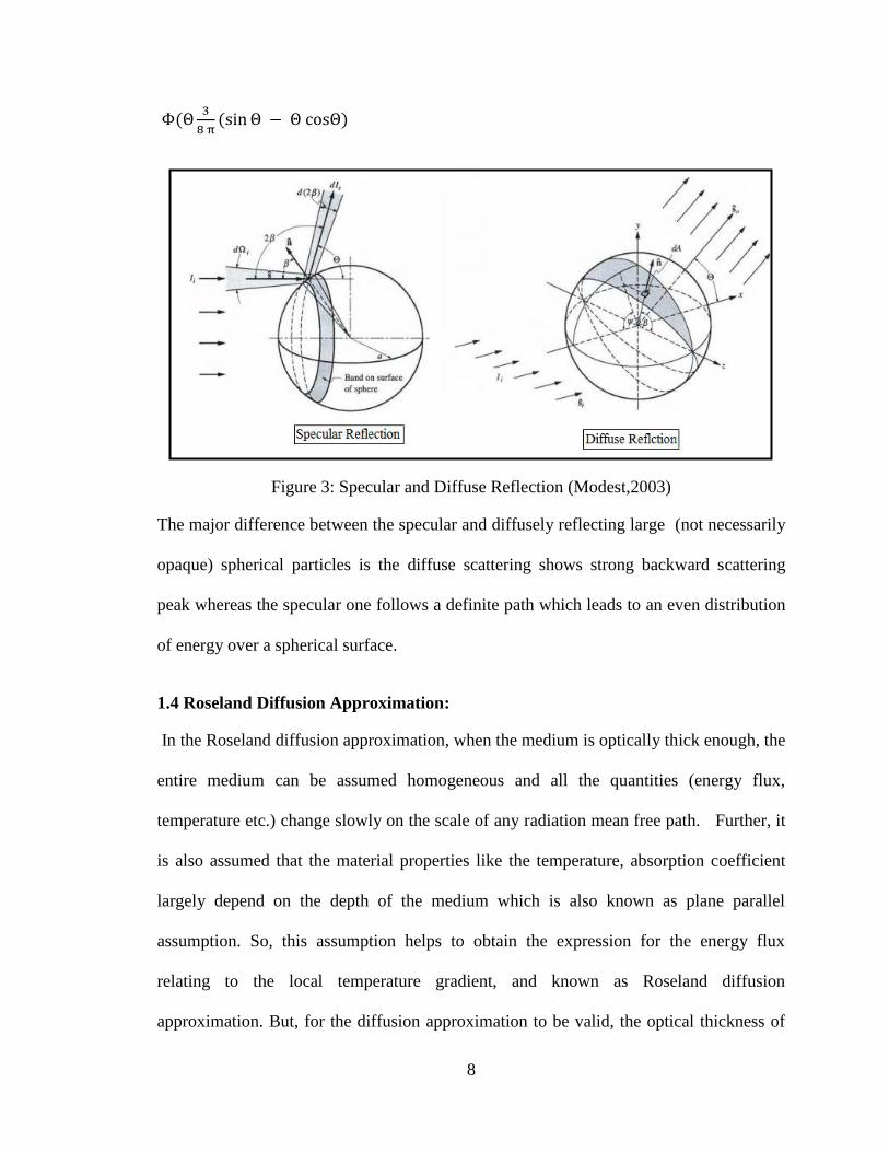
Figure 3: Specular and Diffuse Reflection (Modest,2003)
The major difference between the specular and diffusely reflecting large (not necessarily
opaque) spherical particles is the diffuse scattering shows strong backward scattering
peak whereas the specular one follows a definite path which leads to an even distribution
of energy over a spherical surface.
1.4 Roseland Diffusion Approximation:
In the Roseland diffusion approximation, when the medium is optically thick enough, the
entire medium can be assumed homogeneous and all the quantities (energy flux,
temperature etc.) change slowly on the scale of any radiation mean free path. Further, it
is also assumed that the material properties like the temperature, absorption coefficient
largely depend on the depth of the medium which is also known as plane parallel
assumption. So, this assumption helps to obtain the expression for the energy flux
relating to the local temperature gradient, and known as Roseland diffusion
approximation. But, for the diffusion approximation to be valid, the optical thickness of

9
the bed should be (τo>>1) and dimensionless optical thickness τo = ( σ+ α )L. Where σ is
the scattering coefficient, α is absorption coefficient and L is a length of the bed.
1.5 Introduction to the integro-differential equation in interacting medium.
Figure 4 : Schematic diagram for absorbing, emitting and scattering medium
When an incoming radiation intensity passes through an interacting (absorbing
emitting and scattering) medium, the radiation heat transfer is given by the following
equation (refer, Figure 4).
Where, ,
are solid angles of incident
and leaving radiation intensity.
10
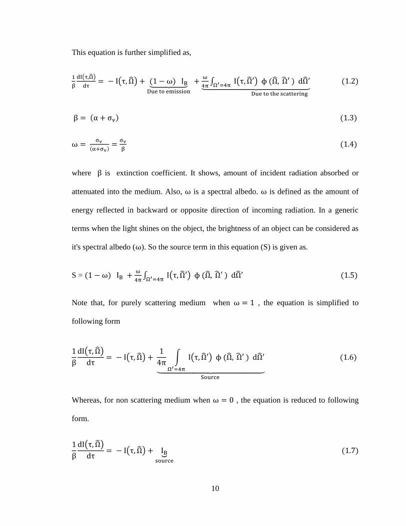
This equation is further simplified as,
where is extinction coefficient. It shows, amount of incident radiation absorbed or
attenuated into the medium. Also, is a spectral albedo. is defined as the amount of
energy reflected in backward or opposite direction of incoming radiation. In a generic
terms when the light shines on the object, the brightness of an object can be considered as
it's spectral albedo ( ). So the source term in this equation (S) is given as.
S =
Note that, for purely scattering medium when , the equation is simplified to
following form
Whereas, for non scattering medium when , the equation is reduced to following
form.

11
CHAPTER 2: RATIONALE AND OBJECTIVE
2.1 Rationale:
Selective laser melting and laser sintering are commonly used processes nowadays in
industry. These rapid manufacturing processes use the laser beam to melt the layer of
metallic powders, and produce the components of complex shapes. Optical thickness of
such powder layer is very thin, up to 100 microns, and the metallic powders can be a
mixture of particles of one or more metals. The metallic powder also has a high
reflectivity which causes the laser beam to travel along a long path into the layer until it
gets completely absorbed in the bed or reflected by the substrate. The layers can have a
large particle up to 50 microns. Hence, along the height direction, a thin layer can only
contain two to three particles at a time. In such condition, the substrate plays a very
important role by absorbing and reflecting the incoming energy.
It’s well known that, metal particles are highly anisotropic scatters due to the large
amount of radiative energy is back-scattered by the opaque particles. Therefore, porous,
particulate bed behaves like a highly anisotropic scattering medium. The results obtained
for the radiation transport in absorbing and anisotropically scattering turbid water bodies
by Daniel et. al.(1979), showed that the use of single point scattering phase function in
the two-flux model produces highly inaccurate results. Further, Brewster and Tien (1982)
demonstrated that for the size parameter (x=1), the error in the results obtained by two
flux method in anisotropic point scattering medium is 10% , and increases up to 40% for
higher size parameters. For the optical thickness (τo >2) the transmittance is under
predicted by 30 to 50%. Moreover, Viskanta and Menguc (1981) also confirmed the
errors in two flux methods in anisotropic medium while working on the radiative

12
properties of pulverized coal and fly-ash. Further in 1991, Singh and Kaviany(1991)
mentioned that the two flux method is incapable of handling the collimated laser
condition for large spherical particles in the packed bed. Gusarov et.al.,(2009), who
studied the radiation transport in thin metallic layers also concluded that, when the
particles in the powder bed are having a reflective properties like a small metallic
spheres, the laser beam penetrates into the powder bed at much higher depths due to the
multiple reflections in the open pore system. They showed that in thin layers the two flux
method considerably over-estimate the deposited energy. The deviation in the energy at
the boundary is due to the high value of porosity at the bed boundary. For the structures
like simple cubic packing the porosity fluctuates rapidly and also approaches to unity as
in between two sub-layers which are discussed in detail in section 4.5. This causes a huge
fluctuation in energy density within the layer.
Analytical models assume the Roseland diffusion approximation, and treat the powder
bed as a homogeneous absorbing and scattering continuum. The Roseland approximation
assumption is only suitable for thick beds. In thick beds particle size much smaller than
the optical thickness of the bed, and the boundary effect can also be neglected.
Sometimes, even for thick packed beds of particulate medium, the analytical models fail
to predict the accurate results for transmission due to the weak intensity transmitted
through the bed. Therefore, for thin particulate layers which are close to the Roseland
optical thickness limit, the analytical models are not capable of capturing the details and
produce the highly unreliable results.
Hence, some concrete model is required to estimate the energy absorbed by thin layers.
The Monte-Carlo Method is very useful in such kind of situations, because it is capable

13
of capturing the minute details at the boundary of thin beds where the Roseland
approximation is no longer useful. It is quite possible to track down the location of the
photon in the particulate bed using current high performance computers, and get good
idea of radiative transport in porous medium. Also, problems are associated with two flux
method for spherically packed thin particulate layer, highly encourage to use the Monte-
Carlo Method. However, the complexity of tracking the individual photons, scattering
phase function in a 3 dimensional systems and large computation time makes the analysis
difficult.
2.2 Objectives:
In order to study accurate radiation transport in selective laser melding process, following
objectives has been set.
1. To build a concrete model to figure out difference in rate of radiation heat transfer
between thick and thin particulate layers.
2. To find out the change in the radiation heat transfer for different type of packing
structures (simple cubic, rhombohedral or random packing).
3. To figure out effect of porosity on the rate of radiation heat transfer in packed beds,
and the transmission using specular and diffuse reflections.
4. To capture the radiative heat flux over the particle surface and the energy absorbed by
the bed.
5. To find out the radiative heat transfer effects at the boundaries using a high resolution
technique.

14
6. To carry out three dimensional simulation of radiative heat transfer analysis in thin
layers.
7. To study the effect of absorbing and reflecting substrates in thin layers
8. To analyze the effect of different laser beam configurations projected over a packed
bed.
9. To figure out the effectiveness of the Monte Carlo method for the radiation heat
transfer in thin particulate layers.
2.3 Theoretical framework for the problem:
Figure 5: Laser beam shining over a porous bed
When the incident laser radiation shines over a powder bed, the total intensity (I)
travelling through the powder bed is taken as sum of defused part ( ) and collimated part
( ). The collimated component also behaves very similar to the diffused component and
satisfies the transport equation.
So, in the original Radiative Transport Equation (RTE) ( equation 1.2), substitute the
following term

15
I = [ Ic + Id
Also, note that the collimated component is defined in form of a heat flux
Ic = [1- ] , Where is a dirac's delta function, which converts
the source in to a point source.
Substituting the equation 2.1 in to 1.2,
After some manipulations we get the following governing equation,
Now before going further it is important to note that for thin layers (bed with low optical
thickness), the intensity of the laser radiation is significantly high. Hence, there will be a
considerable amount of reflection from the substrate. Therefore, it is required to add the
reflected term in our original source term (Source Term s1 in equation 2.3).
Also, the reflected term will be contributed by collimated part , diffused and emitted
parts. The reflected term (source term 2) is given below,

16
+
which is a property of angle of
incident and reflection. If a lambertian reflectance is assumed then the substrate will
reflect diffusively.
Now our complete equation will be
Let's simplify our equation 2.5. By neglecting the term (c) from the source term 2,
because that terms are very small compared with collimated term (b). It is very complex
to figure out the term (a), because diffused component at the substrate i.e is
unknown. Furthermore, using an appropriate boundary conditions and some simple
assumptions, term (b) can be figured out and added as a reflected component in the
equation.

17
So, Let
and assuming perfect reflectance , The
equation can be written as
2.3.1 Two Flux Method to solve the RTE : -
So, by transforming the above equation in positive and negative fluxes,
also , after some simplifications
Forward intensity:
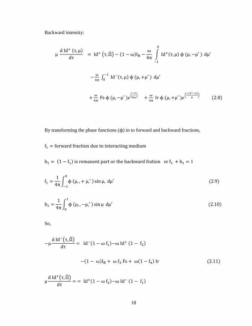
18
Backward intensity:
By transforming the phase functions ( ) in to forward and backward fractions,
or 1
So,

19
The schematic below gives the brief idea of six different components taken in each
equation:
Figure 6: Forward and backward scatted components with collimated laser source and
reflection from bottom surface.
If it is assume that,
1. Contribution from the emissive parts ( ) are negligible compared with the
collimated part and its reflected component ( ). The term can be
dropped from our equations.
2. If the scattering in the bed is isotropic then f1 =f2 and f3 = f4 .
3. Spectral albedo (w) fractions f1 and f3 are constants.

20
Finally, we end up with the following linear coupled equations
And the boundary conditions are = and g

21
CHAPTER 3: LITERATURE REVIEW
3.1 Background on radiative transport in packed bed systems :
The literature review done by Chen and Churchill in 1963, shows the different
approaches and techniques used by various researches in early years for solving radiative
heat transfer problem in packed bed system. Before 1950's the researchers like Nusselt et.
al., (1913), Damkholer et al., (1937) and Argo et al., (1953) treated this problem as an
alternating layers of solid and gas which are perpendicular to the direction of heat
transfer. Roseland et al., (1936) considered diffusion of photons when photon travels in a
random path through a porous medium. Whereas, Hamaker et. al., (1947) successfully
implemented the two flux method for radiant heat transfer using three coupled differential
equations. These works were broadly focused to figure out the expression for function F
in the radiant conductivity ( ) of the medium . Where is the Stefan-
Boltzman constant, d is diameter of the particle in the bed and T is the bulk temperature
of the bed. They came up with different expressions for the function F in relation with
temperature, particle size, mean path free length, absorption cross section and index of
refraction. (Chen et. al., 1963)
A problem of heat transfer by radiation through insulating materials was initially
evaluated by Larkin and Churchill in 1959 using theoretical and experimental
approaches. The focus of their investigation was on the lightweight insulating porous
materials such as styrofoam, polystyrene, polyurethane and fiberglass, which has a large
amount of void space basically filled up with gas. Theoretical part of their work was
basic two flux method which considers forward and backward fraction of radiant energy
travelling through the porous medium. For the insulating materials, they concluded that

22
only 5 to 20% heat transfer takes place through the radiation. In the weakly absorbing
materials, increase in bulk density decreases the radiant heat transfer. Also, when there is
an increase in backward scattering cross section per unit volume of insulation (N) (which
is also a function of scattering coefficient and pore size), the radiation heat transfer
deceases. (Larkin et al.,1959).
In 1963, Chen and Churchill studied the dominance radiant heat transfer in optically
isothermally packed thick beds consists of glass, aluminum oxide, steel and silicon
carbide spheres and irregular grains. They also used two-flux model and compared their
results with the experimental work. Their experimental setup is shown in the Figure 7. In
this setup, the intensity of the heat flux transmitted through a packed bed made up of
metallic or glass particles. The signal is measured at various depths of the bed using the
thermopile detector. The results of their experimental work have been used by many
researchers to compare their theoretical models for a packed bed system. Figure 8 shows
the sample experimental results for the steel spheres by Drolen et. al.,(1987). They also
the derived expression for the function F to determine the radiant conductivity is
Where absorption cross section per unit volume of packing, b is a back
scattering cross section per unit volume of the packing and d is a the diameter of the
particle. They showed that at very high temperatures (more than 1600oF) the radiation
heat transfer is significant from 50 to 85% in thick packed beds consists of large
transparent glass spheres ( up to 5mm thick). Even if for the opaque particles like silicon
carbide, back scattering is a major mechanism for a heat transfer and it is significant up to
33%. So, finally they concluded that the high temperatures and particle size make

23
radiative transport effective regardless the type of material in an isothermally packed bed
(Chen and Churchill, 1963).
Figure 7 : Experimental setup for radiation heat transfer through packed bed systems
(Chen and Churchill,1987).
24
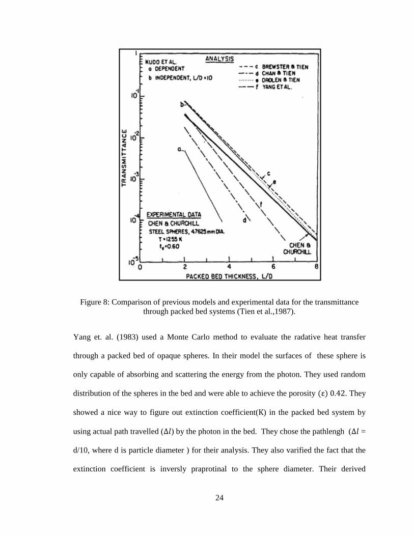
Figure 8: Comparison of previous models and experimental data for the transmittance
through packed bed systems (Tien et al.,1987).
Yang et. al. (1983) used a Monte Carlo method to evaluate the radative heat transfer
through a packed bed of opaque spheres. In their model the surfaces of these sphere is
only capable of absorbing and scattering the energy from the photon. They used random
distribution of the spheres in the bed and were able to achieve the porosity . They
showed a nice way to figure out extinction coefficient( ) in the packed bed system by
using actual path travelled ( ) by the photon in the bed. They chose the pathlengh ( =
d/10, where d is particle diameter ) for their analysis. They also varified the fact that the
extinction coefficient is inversly praprotinal to the sphere diameter. Their derived

25
function (F) for the radiant conductivity (Kr) was
. Comparision of their
model with chen et. al.,(1963) experiments is shown in Figure 8.
Tien et al.,(1987) complied the previous work on scattering in particulate media and
analyzed the dependent and independent theories for packed beds. They pointed out that
size parameter ( ) and clearance to wavelength ratio and volume fraction ,
which is related to the geometric parameter are the most important factors during
the scattering process. Further on the basis of criteria, they classified the
independent and dependent scattering in to two distinct regimes using a size parameter
versus volume fraction curve as shown in the Figure 10 by Tien et al., (1987), however
this criteria is further refuted by Singh et al.,(1991) for packed and fluidized bed.
Figure 9. Independent versus Dependent scattering regimes using the particle size
parameter and the volume fraction. (Tien et al.,1987).

26
For the radiation heat transfer in a packed beds, Singh and Kaviany,(1991) compaired the
independent scattering theory with the direct simulations using the Monte-Carlo
technique. Their analysis was for the opaque, transparent and semi-transparent spherical
particles in the bed. They showed that independent scattering fails drastically for the
lower porosities or packed beds and even when the C/ criteria is satisfied. They also
concluded that the independent theory shows good results for very high porous mediums
( ), but it also fails to predict the behavior at the boundary. With the promising
results given by the Monte Carlo technique they concluded that it is worth for more
research (Singh et. al.,1991).
Solution for the inverse radiation problem for an inhomogeneous medium using a Monte
Carlo technique is discussed by Subramaniam et. al., (1990). In their work, they advised
to use the step isotropic phase function for highly forward scattering particles. They also
pointed out that if the accurate extinction coefficient is known then the results by the
Monte Carlo methods will be more accurate ( Subramaniam et. al, 1990).
The problem of packed beds with large sized semitransparent particles using discrete
ordinate method is solved by Singh et. al., (1991). The results obtained by the desecrate
ordinate method showed a good accord with Monte Carlo method. They also introduced
the scaling factor in order to get the dependent scattering results from independent
scattering method by their optical thickness.
Lu et al.,(2004) compared Reverse and forward Monte Carlo methods for transient
radiative heat transport in non-absorbing, emitting and scattering media. They concluded

27
that reverse Monte Carlo method is very time efficient and quite accurate when compared
with desecrate ordinate method.
Comparison between homogeneous phase and the multiphase approaches for dispersed
media is investigated by Randrianalisoa et.al., (2010) using continuum based approaches.
They found that, in order to evaluate transmittance and reflectance, homogeneous phase
approach is most suitable one. Also for the multiphase approaches, it was difficult to
capture the small details of backscattering in case of transparent and semitransparent
particles. Further, for the large size particles the deviation of radiative properties from the
independent scattering model is significant and ray tracing models such as Monte- Carlo
methods can be more effective in such cases. (Randrianalisoa et. al., 2010)

28
3.2 Background on selective laser melting process:
Selective laser melting (SLM) is a rapid manufacturing process used to build the complex
metallic components by melting the fine metallic powders by high energy laser beam.
Higher mechanical properties are achievable with this process, also the joints-free parts
are stable and less defective compared to the conventionally welded parts. A laser beam
can generate a temperature up to 2000oC, and melt aluminum, titanium and iron based
powders process. A CO2 laser and Nd-yttrium aluminum garnet (YAG) fiber lasers are
used in most machines. The power of laser beam can vary from 25 to 100 Watt, however
some machines can go as high as 500 Watt. Typical thickness of power layer ranges from
20 to 100 microns. (Verhaeghe et. al., 2009). Recent development in SLM machines
shows that some new generation single mode Ytterbium fiber lasers of near infrared
spectral range from 1050-1100 nm are in use for better quality and performance.
Yadroitsev et al, (2010) studied the effects of powder layer thickness, scanning speed,
laser power for a selective laser melting process from a single track method to analyze
stability of laser melting. Their observations showed that high scanning speeds creates
the instabilities and give rise to the balling effect. Optimum scanning speed increases
with increase the laser power and mechanical properties also vary significantly with
change in the direction of scanning (Yadroitsev et. al., 2010).
Various important parameters and their effect on melting process has been discussed by
Thijis et. al., (2010). He mentions that the laser beam creates a molten pool, and due to
the surface tension the pool takes a cylindrical or semi-spherical shape. Fragmentation of
remelted tracks, instabilities like distortions, porosities and the balling effects during the
solidification are the well-known defects of SLM process. The optimal parameters such

29
as laser power, thickness of layer, scanning speed and substrate material are the critical
factors for the stability of the process.
Gusarov et al.,(2004) used a two flux method, developed a model for radiation heat
transfer metallic powders used in selective laser melting process. Using dependent
scattering they studied specularly and diffusely reflecting particles. They concluded that
dependent scattering can be neglected while evaluating phase function and albedo for
metallic powders. Also due to the several reflections in the porous bed the laser energy
can transmit at higher depths in the powder beds. It is clear that the absorption capacity of
the powder bed increases with increase in the layer thickness. They also noted that,
specular reflection gives higher values for energy density and absorptance than the
diffused reflection due to the dominance of backward scattering in specular reflection
(Gusarov et al., 2004).
Further in 2010, the numerical analysis given by Gusarov et al., (2010) for a case in
which the radiation heat transfer in powder beds with a substrate irradiation is evaluated.
They showed that for the smaller thickness of the powder layer the absorbtivity of the
substrate is significant but it shows the local maximum value as the increase in optical
thickness. As it is known that higher reflection rates reduce the absorption capacity of the
bed but they are required for the uniform heating of layer ( Gusarov et al., 2010).
30
CHAPTER 4: BED GENERATION METHOD AND MONTE CARLO
PROCEDURE
4.1 Simulation of packed beds:
The packed bed usually consists of heterogeneous mixture of randomly filled solid
particles of spherical, cylindrical or irregular shapes. They are used in many
manufacturing as well as chemical processing applications such as selective laser
melting, laser sintering high performance cryogenic insulations, pebble bed in nuclear
reactors etc. (Yang et. al., 1983).
It is known that the packing structure of the porous bed, which is a function of
size of particle ) and porosity ( ) , largely affects the rate
and mechanism of heat, mass and momentum transfer in packed beds. Traditionally, three
types of packing structures have been used by the previous researchers; these structures
are random closed, random loose and random poured (Reyes et. al., 1990). These palings
structures were classified on the basis of porosity or a void fraction. Void fraction is
defined as the fraction of packing volume that consists of voids, whereas solid fraction is
obtained by subtracting void fraction from the unity (Yang et al., 1983). Physically the
solid faction is the density of the bed. The number of particles in contact is also one of
the most important properties which affect the overall structure of the bed. The
probability of number of contacts a particle can have in the bed is defined as the number
frequency by Yang et al., (1983). The large number of neighbors increases the number of
interactions. Hence, it is worth putting some efforts on the various clustering features of
the bed.

31
Several efforts have been made by researchers in past to artificially simulate packed beds.
Computer code originally created by Jodry et al., (1981) can evaluate the solid fraction
and coefficient of extinction in randomly packed beds. The code has been used to
generate a randomly closed packed bed of density 0.64. This code was further modified
as PACKUET and used by Yang et al., (1983) for rigid spheres with same diameters and
fixed porosity of 0.42 in their analysis. Later on, Singh and Kaviany et al.,(1990) also
used PACKS which was the improved version of PUCKET and able to achieve a variable
porosity arrangement varying from 0.42 to 1. (Singh et al.,1991).
The purpose of this study is to analyze the effect of heat transfer within thin metallic
layers having a particle size applicable for the powder bed of laser additive
manufacturing. The artificial packed beds of spherical particles have been created using
MATLB program. The particles in the packed beds can be arranged in different ways to
make the beds more realistic. The variation in particle sizes and the inter-particle
clearance can be adjusted in order to study the behavior of the beds. The program can
generate simple cubic, rhombohedral and randomly packed beds of spherical particles.
The effect of reducing the layer thickness to the radiation heat transfer is also studied.

32
4.2 Types of packed beds:
4.2.1 Simple cubic packing of spheres:
The simple cubic packing arrangement is
shown in Figure 10. This is the most simple
configuration acheiced by placing the
particle precisely above previvously
generated particle. In this type of packing,
the number of layers in the bed (N) are
exactly equal to the L/d ratio. Where, L is
the thickness of the bed and d is the particle
size. All the particles in the bed are
spherical, and have equal diameters. The
maximum volume density can be obtained form this type of arrangement is 0.535. It is
possible to increase the horizontal and verticle distance between the two particles (in x,y
and z direciton) to obtain high porous bed, however increasing the distnce in z direction
will keep the particles hanging in the air. The focus of the study is on the radiative heat
transfer simulation of packed beds contains small metallic particles. When the one or
more particles are not touching each other, the condition doesn't look appropriate for the
analyis, however such hanging configuration is suitable for certain multi-phase flow
cases, such as the clouds and different planetory atmosphes.
Figure 10: Square or simple cubic packing
of spherical particles

33
4.2.2 Rhombohedral Packing of spheres in the beds :
Rhombohedral packing is the most dense packing structure can be achieved when the
equal diameter (d) spherical particles are
packed in the cube. The distance between the
two layers is given by The
construction of a rhombohedrally packed bed
is depicted in Figure 11. This type of packing
is generated using layer by layer approach.
The volume density of such type of packing
arrangement can be up to 0.74.
4.2.3 Random Packing of spheres in the bed:
A close look at the metallic power beds
shows that most of the particles are of
unequal sizes. Their arrangement is also not
uniform. Sometimes two or more particles
touch each other. The top boundary of the
bed is also irregular and particles unevenly
pop out from the top boundary. Such type of
configuration is also known as random
packing. A typical random packing is
shown in Figure 12.
Figure 11:Rhombohedral Packing of
spherical Particles.
Figure 12: Random Packing of spherical
particles in cube.

34
4.3 Procedure used to create the random packing:
The algorithm given below creates the random packing of particles in a cubic space.
These particles may touch each other but they cannot overlap. Particles can be supported
by other particles depending on the randomness in their generation. A unique fixed center
algorithm approach was adopted to facilitate various configurations of random packing in
this study.
1.The MATLAB code initially generates fixed mesh for the centers using the given
diameter range ( ) , the size
of the bed and inter-particle clearance in all three directions. The mesh is generally very
dense and smaller than the diameter of the particle.
2. After fixing the location of centers, the program randomly generates first particle
within range at the first center.
3. Further, the program generates another center at the next specified location (usually at
(d1+d2)/2 in x direction) within the given range of diameters. If the newly generated
center lies inside any previously existing spheres, then the program moves to the next
center.
4. If the center doesn't fall inside any diameter of any previously generated spheres then
the distance between the all previous centers and the newly generated center is calculated
to figure out the closest center and has a largest diameter.
5.If the newly generated diameter interacts with that maximum closest diameter then the
program modifies the diameter to its minimum set value or moves to the next center.

35
6.If the newly generated diameter is too far away from the sum of maximum closest
diameter and inter particle clearance then also the program modifies the diameter to its
maximum set value or can move to the next center.
7. Probably function also helps generate the smaller or larger size spheres, which are not
within the range but will help fill out the void space.
8. Figure 13 shows the different types of random packing configurations obtained using
the program.
Figure 13: Different packed beds arrangements generated using random packing
algorithm.
Similar type of approach is used for the generation of rhombohedral packing. For the first
layer, the distance between the two particles (h) is simply set to in x and y
directions. For second layer, the sphere center to center distance is again increased by
in z direction and the remaining sphere are generated. The same action is
repeated for remaining layers to get a complete rhombohedraly packed bed.
36
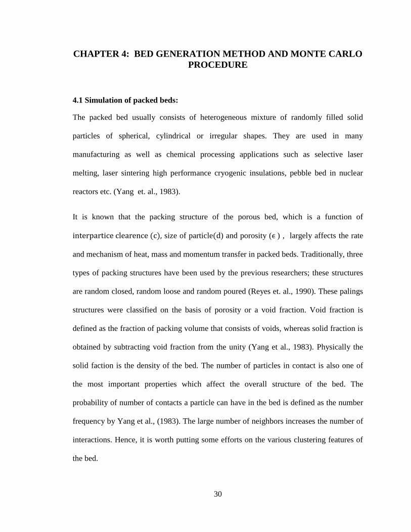
4.4 The schematic diagram for the randomly packed bed program:
Figure 14: Schematic diagram for random packing algorithm
This algorithm generates the particles of random sizes within the specified diameter
range. Also, based on the assigned probability value, there exist some chances of having
the smaller or larger particles in the bed. The input diameters can be adjusted to produce
a simple cubic structure. Also, the particles may or may not touch each other depending

37
on the clearance provided, however every particle can be set to touch at least a one
closest neighboring particle in the bed.
4.5 Porosity of the packed beds
Porosity of the bed is one of the most important factors in radiation heat transfer. Porosity
increases with the interparicle clearance. A high value porosity increases the dominance
radiation heat transfer over a conduction in a porous system.
Figure 15 : Porosity calculation in four simple cubic and rhombohedral spheres
The simple cubic type has a cube shaped structure with the spherical particle at the each
corner as shown in Figure 15. A 0.5 x 0.5 x 0.5 mm sized bed is generated using the
simple cubic method. The bed is packed by using 0.1 mm diameter spherical particles.
Figure 16 : 0.5 x 0.5 mm simple cubic bed with 0.1mm particle size
38
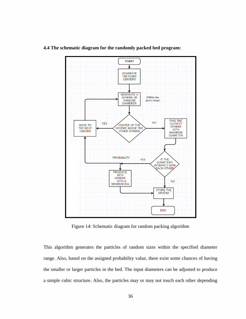
The porosity of this configuration is plotted as a function of bed thickness in Figure 17.
It can be seen from the plot that value of porosity in cubic packing fluctuates very
largely. After each layer the porosity approaches to one. This happens due to the point
contact between the two adjacent layers.
Figure 17 : Porosity as a function of bed height in a simple cubic packing configuration
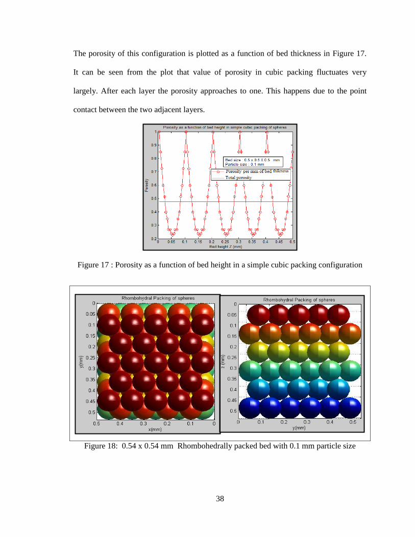
Figure 18: 0.54 x 0.54 mm Rhombohedrally packed bed with 0.1 mm particle size

39
In approximately 0.54 mm sized cube. The porosity obtained from this arrangement is
plotted in Figure 19. The plot shows that, the rhombohedral packing porosity fluctuates
form its mean value but does not reach to unity like simple cubic arrangement. Also, the
minimum porosity points have a value close to 0.25.
Figure 19 Porosity as a bed height in rhombohedral packing
The random packed bed made up of particle size between 0.07 to 0.1 mm and has a
dimensions of 0.5x0.52x0.54mm is shown in Figure 20, and the porosity plot is
illustrated in Figure 21. The local value of porosity (red line) in the main body of the
filled space remains below the mean value of the bed which is 0.58. This indicates that
the actual value of the porosity inside the bed in less than the average value. The
deviation is because of the highly irregular top layer and bottom layer.

40
Figure 20 : 0.54 x 0.52 x0.54 mm randomly packed bed with 0.7 to 1 mm particle size
Figure 21: Porosity as a function of bed height in random packing
4.6 Monte Carlo Method :
Study of radiation heat transfer for the particulate medium has been conducted by many
researchers in the past. Numerous models have been developed since then to simulate
heat transfer in packed beds. The Monte Carlo technique is a one of the numerical
methods based on the statistical approach. This Method has been proven very effective
for an evaluation of radiative energy transport.

41
The implementation procedure of Monte-Carlo Method in this study is given below
The particles in the powder bed are assumed perfect spheres; however, the
diameter of the particles can be different.
The collimated laser beam strikes perpendicular (0o) to the bed or at different
angles (30o, 45
o or 60
o) to the z- axis of the bed. Further, the beam can also be
adjusted for non-collimated way.
100,000 photons bundles are fired and traced inside the bed
The input laser beam can have a uniform, conical or Gaussian distribution. The
Gaussian distribution is achieved by program known as guassianbeam.m
The diameter and the intensity of the laser beam can be adjusted as per the
requirements. For this analysis beam 50 W to 100 W power beams are used.
Each photon in the bundle is fired at the different locations and the intensity at the
top boundary of the bed (x,y,0). This is achieved by using the sprialinput.m
MATLAB function. This function initially fires the first photon exactly at the
center of the bed and then fires the remaining photons in going spirally outward
manner as shown in Figure 22.
Figure 22: Spiral Input function for laser source

42
The x, y and z dimensions of the bed are divided into number of grid sizes nx, ny
and nz respectively.
For this evaluation, 100 x 100 x 100 grid points are selected. The minimum grid
dimension in z-direction is known as a resolution of the system. For example, if
the depth of the bed is 1.5 mm with 100 gird points, then the resolution comes out
to be 0.015 mm or 15 microns.
The photon travels a length of resolution at the given directions. After every
travel, the program checks for the location of the photon.
If the photon is found inside the particle, the program quickly figures out it's
point of entry, and runs an another subfunction (storephoton.m) to store the
energy at that point on the spherical surface.
The original energy of the photon is reduced by subtracting the absorbed energy
and the remaining energy is assigned to the photon
After that the photon is set back to the original point of intersection and then it is
scattered using the scattering phase function.
Either diffused or specular reflection is used to mimic the scattering mechanism in
the spherical particle.
If the photon reaches to the bottom surface of the bed, it is either absorbed
completely or partially, and reflected back to the bed.
If the photon comes out of the bed from any other direction except the bottom, it
is not tracked further but the bed in x and y directions are chosen sufficiently
large to avoid the energy loss though the sides.

43
The photon bundles are tracked inside the bed as long as it gets completely
absorbed by the particles or come out of the bed.
After the last bundle, the total energy of the bed is normalized by dividing the
stored energy by number of photons fired.
The schematic diagram of the complete Monte Carlo procedure is shown in
Figure 25.
4.7 Properties of metallic powder bed while using the Mote Carlo simulation:
4.7.1 Scattering:
As discussed earlier, in a specular reflection (Figure 23) the photon gets reflected
in exactly opposite direction to the angle (β) made by direction vector of
incoming photon and the surface normal (n) at that point of intersection, however,
the azimuth angle is chosen randomly between 0 to 2 in a way that it won't
interact with the same sphere after the reflection. The surface normal at any point
(x1,y1, z1 ) is given by the following formula.
Figure 23: Specular Reflection

44
In diffused interaction, the reflection given by the phase function formula
given below.
Figure 24: Scattering phase function for diffuse reflection generated using Henyey-
Greenstein phase function (at g = -0.7) using random numbers.
The phase function plot (Figure 24) shows that the fraction of incident radiation
reflected in backward and forward direction. From Figure 24 it is visible that the
large area under the curve (μ from -1 to 0 ) signifies the dominance of back
scattering over a forward scattering in diffuse reflection.
This type of backscattering can be also achieved by using Hanyey Greenstein
(HG) Phase function (red points shown in Figure 24 ). The HG phase function is
discussed in detail in the next section.

45
4.7.2. Photon path Length :
The path length is defined as the attenuation of the light with respect to the optical
distance travelled. The path length in the porous bed is given by the probability density
function.
P (l) =
(4.3)
Different ideas have been proposed by different researchers for the attenuation of
radiative energy in Monte Carlo radiation models. If the bed is made up of homogeneous
medium, like a skin layers or water, the photon uniformly loses its energy while
travelling inside such internal scattering mediums. Hence in such models, the photons
are scattered as point scatterers and they are attenuated using the equation 4.3.
However, in the present study, the model consists of comparably large metallic particles
than water molecules. The photon only loses its energy when it comes in contact with
surface of the particle. It keeps travelling in the specified direction until it is fully
attenuated.
In this model, the minimum resolution size of the grid in z direction is taken as a
constraint path length of the system. It is given by the following equation
l = Lz/nz
Where, Lz is optical thickness of the material and nz is the number of grid points in Z
direction. The idea behind keeping the path equal to the resolution of the grid is quite
simple. Firstly, resolution is the minimum length scale of this system up to which it is
possible zoom in and the track the photon. Secondly, the particles in the bed are relatively
large. Therefore it is assumed that if the photon comes in contact with the particle, it will

46
definably interact with the particle. It will not happen that the photon skips the particle in
the incoming direction and moves to the next particle. So, it is possible to assume that
the extinction coefficient is only a function of type packing arrangements and the particle
geometries.
The reduction in the path length for opaque ( only absorbing and reflecting ) particles
seems quite unfeasible. If the particle surface is smooth enough then remaining
unabsorbed energy of the photon will always travel away from the sphere. In Euclidian
space-time, the outward unit normal vector (n) coming from the spherical geometry will
never intersect the same sphere. Hence, for the shorter path lengths the photon will stay
in the same node or grid point for longer time and will lose the energy more than once at
the same point.
4.7.3 Movement of photon in the particulate medium :
The photon is reflected using the direction cosines ( ). Where the angle
changes is from 0 to and the azimuthal angle 0 to radians is
shown in Figure 24.
;

47
Figure 25: Coordinate system for packed bed
The initial location of the photon is set at the top boundary (z = 0 ) and at the center of x
and y coordinates of the bed (at = and = ).
For the collimated type of beam configuration the azimuthal direction is fixed at
, and then the program fires the collimated rays at the different angles assigned in
.
The next location of the photon in the Cartesian coordinate system is updated using
following equations,
Where are the old locations in x, y and z directions.

48
For the present study the following boundary conditions are considered for the bottom
surface of the bed.
1. Perfectly reflecting boundary like a mirror
2. Completely absorbing (black) boundary
3. Partially absorbing boundary.
The substrate reflection is very important component in a thin layer analysis. In a
selective laser melting, the base surface of the powder layer is not smooth. Therefore, the
reflection from the bottom surface is assumed independent of incoming angles of the
photon. The Lambardian type of reflection is quite good approximation for present study.
The cosine components taken for reflection are and R
4.7.4 Reflection from the base of thin layers:

49
4.7.5 The schematic diagram for Monte Carlo method
Figure 26: Schematic diagram for Monte Carlo Method.

50
4.8 Laser Power Sources:
Figure 27 Collimated and Diffuse source
For the present analysis, two major configurations of the laser source are generated using
the MATLAB program. The power source is either located exactly at the center of the
spherical particle or at the slight offset locations form the centers. The power source
consists of bundle of photons, which are fired one by one in to the bed based on the value
of their intensity at the respective points (at x and y locations).
Figure 28: Gaussian source over a packed bed

51
The Normal distribution function is used to simulate the Gaussian power source. The
50 Watt power Gaussian beam is shown in Figure 29 . The dimensions of the bed are
1mm x 1mm.
Figure 29: Gaussian power source for laser beam (100 W) , 0.4 mm diameter
Figure 30 shows the uniformly disturbed circular laser beam of 50 W with 0.4 mm
diameter over a 1mm x 1 mm size bed . For the equal diameters, the uniformly
distributed plane circular source contributes more power than a Gaussian source.
Figure 30: Uniformly distributed source (100W), Diameter: 0.4 mm

52
CHAPTER 5: RESULTS
In the present study, three dimensional simulations of different types of scattering
mechanisms on thick and thin packed spherical particulate beds have been carried out
using the Monte-Carlo technique. Some images have been captured directly from the 2d
simulation in order to visualize and understand the scattering mechanism in the packed
bed system. The conditions, y is set to y/2 and are imposed on the 3d
simulation in order to get these 2d simulation images.
Figures 32 & 33 show the mechanism of specular and diffuse reflection over surfaces of
spherical particles. The symmetric image in specular reflection shows the definite
behavior and fixed path followed by photons in the medium. This is because of the angle
of the reflection is exactly opposite and equal to the angle made by surface normal and
the incident radiation. If the surface of the spherical particle is very smooth, then the
specular reflection is possible. However, if the surface of the particle is rough then the
surface normal points out to a random direction, and the photon is reflected to some
arbitrary direction with a condition that it doesn't
strike the same particle.
The another important point to notice about the 2d
simulation is when the particles touch each other, the
photon can barely pass or even may not pass to the
second layer. This is not true for the 3d simulation.
In the three dimensional system, there is always an
open passage exists between two adjacent layers
Figure 31: Transmission of
radiation in simple cubic
packing

53
which will allow photons to pass through the gap and transmit energy to the next layer
as shown in Figure 31. Let's define this gap as an 'open pore system'. Now it is clear that,
the collimated rays can penetrate the simple cubic bed at very large depths, however, 2d
evaluation for packed sphere system can create large errors.
Figure 32: 2d Simulation for diffuse reflection with (~ 40 photons)
Figure 33: 2d Simulation for specular reflection with (~ 40 photons)

54
It is discussed in the earlier sections that if the size parameter (x) is very small (1 >> x)
the particle follows the Rayleigh scattering. Studies have shown that, small metal
particles have strong forward scattering peaks due to the diffraction. A very small
aluminum particle (1 >> x) shows an isotropic scattering behavior. For the opaque
spheres like an aluminum particles, it is very difficult to simulate diffraction and generate
the forward or isotropic scattering behaviors in a packed sphere systems, however, the
efforts has been made to replicate the actual process of 'small particle scattering' using
Hanyey- Greenstein phase function . It is given by the following equation:
Where, g is the variation parameter (-1 < g <1) and is scatted angle.
In this method, as soon as a photon comes in contact with a particle, its energy is
absorbed at the surface of the particle based on the reflectivity of spherical material and
remaining energy is reflected towards angle generated by the Henyey - Greenstein phase
function. Basically, the scattering angle is generated from the center point of the particle.
Even though the simulation shows the moment of photon from the center of the sphere,
the particles are assumed completely opaque and path travelled by photon inside the
particle is not related to any type of internal transmission.
Simulation result for the Isotropic scattering in packed spherical packed bed is shown in
Figure 34. This is achieved by the choosing the variation parameter g = 0 in the phase
function equation (5.1). By using random numbers between 0 to 1 and the
rays are scattered almost equally in forward and backward direction.

55
Figure 34 : 2d simulation for Isotropic scattering in packed spherical bed using
Henyey-Greenstein Phase Function (g = 0)
Figure 35:2d Simulation for backward scattering in packed, spherical beds using
Henyey-Greenstein Phase Function (g = -0.7)

56
Figure 36: 2d Simulation for Forward scattering in packed beds using Henyey-Greenstein
Phase Function (g = + 0.7)
When variation parameter (g) is adjusted to negative value, the phase function gives
strong backward scattering peak and vice versa. Figure 35 & 36 show the backward and
forward scatterings obtained in simulation using the variation parameter (g) = - 0.7 and
(g) =+0.7 respectively.
It can be also observed for large particles that the diffuse reflection always shows a
strong backward scattering, and most of the energy is reflected in backward direction.
Therefore, the variation parameter (g) = -7 has been adjusted in such a way that backward
scattering obtained by the Greenstein function closely matches with the diffuse reflection.

57
5.1 Analysis of Radiative Transport in Thick Particulate Beds -
5.1.1 Comparison with previous MC models and experimental work.
A very few experimental results are available for evaluation of radiative transport in a
packed sphere system. Figure 37 shows the comparison between the results obtained
using the present Monte Carlo method and the experimental data obtained by Chen and
Churchill (1963). The results of previous studies conducted by Singh and kaviany (1990)
and yang et al.(1983) are also included in this plot. During the experiments, the diameter
of a steel particle was taken as 0.476 cm and the temperature (T) was 1366K. For the
theoretical purposes, the emissivity value suggested by Breswster et. al., was 0.4. The
same emissivity has been used by Singh and Kaviany for their studies, and also in the
present work. The reflectivity is taken as 0.6. The table given below shows the input
parameters used for current analysis.
Table 1: Input parameters for validation case (Thick bed)
Input Values Packed Bed
Type of bed
Configuration Random Packing,
Scattering Mechanism Specular Reflection
Optical thickness and Bed
dimensions (X,Y,Z) and
grid size
4 x 4 x 5 (cm) and (100 x 100 x 100) grid points
Diameter of the particle 0.44 - 0.47 cm
Porosity 0.52
Reflectivity 0.6
Emissivity of Particles
(E) 0.4
Laser (Type, diameter ) Uniform source, 0o collimated ,
Type of Substrate Perfectly absorbing ( = 0)
Photon path Length Resolution
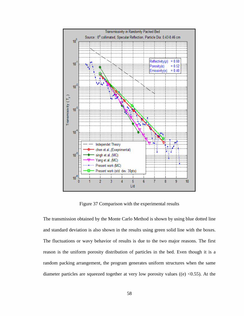
58
Figure 37 Comparison with the experimental results
The transmission obtained by the Monte Carlo Method is shown by using blue dotted line
and standard deviation is also shown in the results using green solid line with the boxes.
The fluctuations or wavy behavior of results is due to the two major reasons. The first
reason is the uniform porosity distribution of particles in the bed. Even though it is a
random packing arrangement, the program generates uniform structures when the same
diameter particles are squeezed together at very low porosity values ((e) <0.55). At the

59
end or at the beginning of each layer the porosity reaches to very high value and there is
insufficient area available for the absorption of the energy. The second logical reason can
be given is, during the specular reflection, photon always follows a predefined path
which creates a localized energy absorption points and produce a non-uniform energy
distribution over a sphere. This can be reduced by either using diffuse reflection and
increasing number of grid points or increasing the number of photon packets. Due to the
computing limitations and time constraints the grid size is fixed to 100 points in x y z
directions and number of packets used are 100000.
Another important issue with the results obtained from the Monte Carlo procedure is the
top and bottom boundaries of the bed where porosity almost approaches unity. In a
randomly packed bed, the particles arbitrarily pop out from the top layer of the bed.
Sometimes, a laser beam finds a complete particle exactly below it or sometimes a part of
it. This creates some differences in the profile obtained at the boundaries of beds even for
the same input conditions and equal porosities. This can be taken cared by using a proper
beam diameter and a particle size. However, this situation is very close to reality, and the
behavior of photons at the boundaries cannot be challenged.
Further, in order to understand the trend of fluctuation for thick beds and to obtain the
readable results, the weighted average is used by Singh and Kaviany,(1991). However,
small weighted averages also fluctuate due to curvy and sinusoidal type profile and the
unknown number of layers in random packing, whereas large weighted averages
includes top and bottom boundaries and makes the results deviate largely from the true
profile obtained using Monte Carlo method. Another possible alternative is the 'thick bed
approximation'. This assumes that the bed is thick enough to neglect the effects at the

60
boundary, so that the actual transmission profile for thick bed can be obtained. Therefore,
for thick bed approximation, some data points at the top and at the bottom boundaries can
be neglected. The weighted average starts from the maximum transmission point of the
first layer and ends with the maximum transmission point at the last layer. Even though it
is pointed out by Singh and Kaviany (1991) that the Monte Carlo procedure lie to some
extent, thick bed approximation stands as a valid argument for averaging and obtaining
mean profile (green squared solid line Figure 36). Furthermore, the proximity of actual
Monte Carlo profile (blue dotted line in Figure 36) to the experimental results (red solid
line) gives good confidence over Monte Carlo procedure. The independent theory or two
flux method (black dotted line in Figure 36), falls short results in predicting a radiative
heat transfer in packed spherical opaque bed.
Yang et. al.,(1983) used the diffuse source boundary condition for the problem, which is
also pointed out by Singh and Kaviany,(1991). Due to the diffuse source at inlet
boundary the laser beam extincts much faster, and leads to a significant difference in rate
of transmission when compared with experimental results. However, in the present
Monte Carlro simulation, the collimated source at the inlet boundary takes care of this
issue. The laser beam hits the top boundary at an angle of 0o
to z axis, and travels along
the depth of the bed until it hits the first particle which also increases the rate of
transmission.
Finally, the emissivity of the steel spheres used is unclear due to oxide coatings (Chen
and Churchill), however, for the present case emissivity (e= 0.4) gave the fair results.

61
5.1.2 Effect of different scattering mechanisms (Simple Cubic packing)
Lot of energy has been spent on the implementation of different types of scattering
mechanisms. The effect of these scattering mechanisms over a packed sphere system is
studied in this section. Following input parameters has been considered during the
analysis.
Table 2: Input parameters for simple cubic bed
Input Values Packed Bed
Type of bed Configuration Simple cubic Packing,
Scattering Mechanism Specular / diffuse/ Isotropic/ Forward and
Backward Optical thickness and Bed
dimensions (X,Y,Z) and
grid size
0.4 x 0.4 x 0.8 (mm) and (100 x 100 x 100) grid points
Diameter of the particle 0.1 mm
Porosity 0.476
Reflectivity 0.7
Laser (Type, diameter ) Uniform source, 0
o collimated , 50W,
diameter = 2.5 mm
Type of Substrate Perfectly absorbing ( = 0)
Photon path Length Resolution
It has already been discussed in the introduction section that metal particles are
considered large when the size parameter is x > 10. If the diameter of the particle is
assumed 100 microns then size parameter (x = ) will give the wavelength of the
laser beam greater than 31.4 µm. As the wavelength increases with respective to the
diameter, the isotropic scattering or the forward scattering can be more effective. For the
selective laser melting processes, the wavelength of the laser beam usually varies from 1
to 10 µm. This gives the diameter of the particle (d) > 3.18 µm so that the particle to
become large. Therefore, for the particles which are larger than d = 30 to 40 µm the

62
specular or diffuse reflection is effective, whereas for the extremely small particles the
Henyey Greenstein function can be applied.
Figure 38 Radiative heat Transfer in simple cubic arrangement
From, Figure 38 It can be clearly seen that there is no huge difference between the
results obtained using specular or diffuse reflection. However, the different slopes of
specular reflection slightly high transmission rate to the diffuse reflection in the porous
beds. Another interesting fact showed by the results is that the specular and diffuse
reflection falls between the range of isotropic (g =0) and backward scattering (g =-0.7)

63
regimes. It is quite clear from the result that, both specular and diffuse reflection show a
high backward scattering behavior. The forward scattering results(g =+0.7) shows
extremely high transmission, which is quite expected. At present, no experimental data is
available to compare the results for this section for extremely small particles in thick
layers. However, the results are compared with Sing and Kaviany (1991) for specular
reflection with the same input conditions. The specular and diffuse reflection scattering
mechanisms results from the present analysis show good harmony with their results.
Finally, the Heyney Greenstein phase function to replicate the forward, backward and
isotropic scattering in extremely small particulates and thick bed, needs a set of
experimental data and for validation. Until then the soundness of the modified part is
questionable. The results for this part are obtained just out of a mere curiosity.
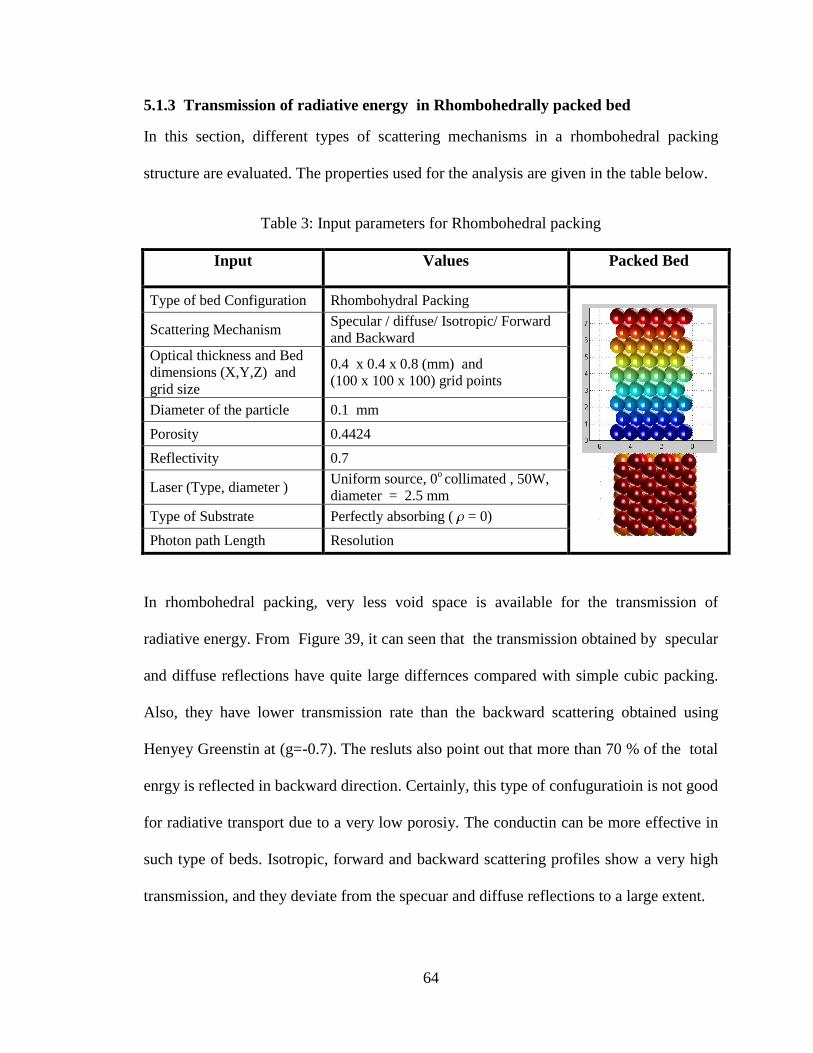
64
5.1.3 Transmission of radiative energy in Rhombohedrally packed bed
In this section, different types of scattering mechanisms in a rhombohedral packing
structure are evaluated. The properties used for the analysis are given in the table below.
Table 3: Input parameters for Rhombohedral packing
Input Values Packed Bed
Type of bed Configuration Rhombohydral Packing
Scattering Mechanism Specular / diffuse/ Isotropic/ Forward
and Backward Optical thickness and Bed
dimensions (X,Y,Z) and
grid size
0.4 x 0.4 x 0.8 (mm) and (100 x 100 x 100) grid points
Diameter of the particle 0.1 mm
Porosity 0.4424
Reflectivity 0.7
Laser (Type, diameter ) Uniform source, 0
o collimated , 50W,
diameter = 2.5 mm
Type of Substrate Perfectly absorbing ( = 0)
Photon path Length Resolution
In rhombohedral packing, very less void space is available for the transmission of
radiative energy. From Figure 39, it can seen that the transmission obtained by specular
and diffuse reflections have quite large differnces compared with simple cubic packing.
Also, they have lower transmission rate than the backward scattering obtained using
Henyey Greenstin at (g=-0.7). The resluts also point out that more than 70 % of the total
enrgy is reflected in backward direction. Certainly, this type of confuguratioin is not good
for radiative transport due to a very low porosiy. The conductin can be more effective in
such type of beds. Isotropic, forward and backward scattering profiles show a very high
transmission, and they deviate from the specuar and diffuse reflections to a large extent.
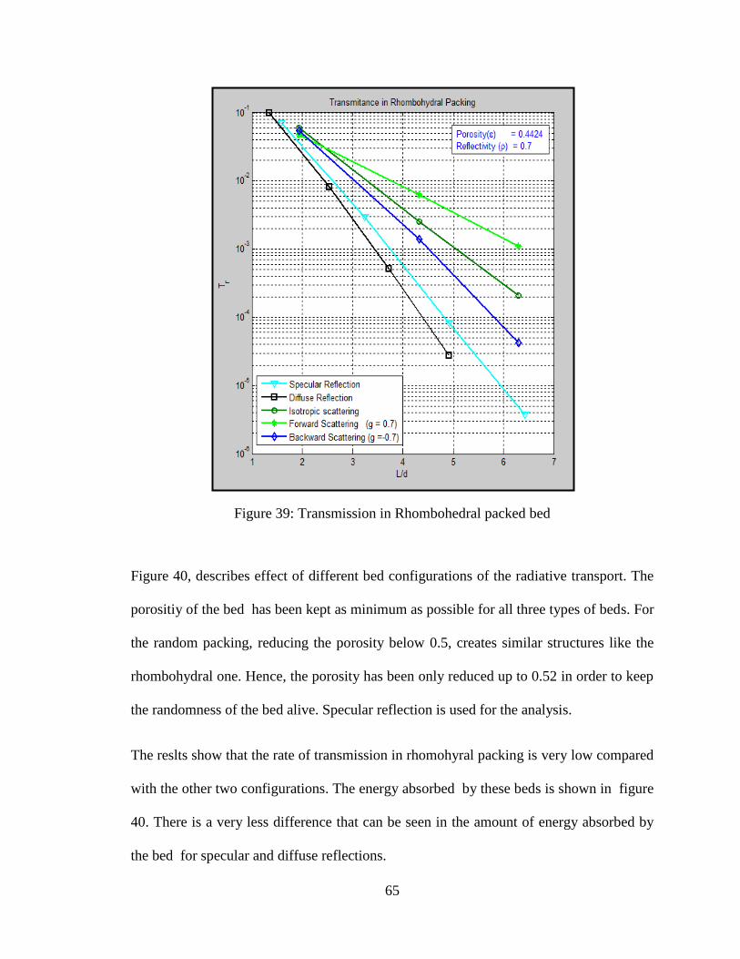
65
Figure 39: Transmission in Rhombohedral packed bed
Figure 40, describes effect of different bed configurations of the radiative transport. The
porositiy of the bed has been kept as minimum as possible for all three types of beds. For
the random packing, reducing the porosity below 0.5, creates similar structures like the
rhombohydral one. Hence, the porosity has been only reduced up to 0.52 in order to keep
the randomness of the bed alive. Specular reflection is used for the analysis.
The reslts show that the rate of transmission in rhomohyral packing is very low compared
with the other two configurations. The energy absorbed by these beds is shown in figure
40. There is a very less difference that can be seen in the amount of energy absorbed by
the bed for specular and diffuse reflections.

66
Figure 40 Transmission in Different bed configurations (Specular Reflection)
The plots shown in Figure 41 indicate that the energy flux passing through the random
bed is much higher compared with the other two types of beds. This can be an effect of
little higher porosity in the random bed. Tin order to shed some more light on this issue,
the effect of porosity in the random bed configuration is studied in next section.

67
Figure 41:Energy Absorbed by the beds with different types of packing arrangements
5.1.4 Effect of porosity in thick particulate beds
The effect of porosity on the radiation transport
in packed spherical system is analyzed in this
section. The variation in porosity for simple
cubic bed is obtained by increasing or decreasing
the clearance between two adjacent layers
vertically and horizontally (Figure 41). For
randomly packed beds, the porosity is adjusted by
reducing the number particles and their
diameters. Figure 42 a & b are plotted to see the radiative energy flux and the ratio of
absorbed energy to the total absorbed energy by the bed at different porosity values. The
specular reflection is used during this evaluation, and the substrate is kept completely
absorbing. The area under the curve in the absorption profile shows the distribution of
absorbed energy by the bed. For very higher porosities, the energy absorption is not
uniform and the maximum absorption of energy takes place at the random places where
Figure 42 Substrate Reflection
simulation
s

68
the particles are located. This happens because of the collimated nature of the beam and
the less number of particles in bed. So, most of the energy is absorbed at the particles
close to the top boundary of the bed and remaining most of the remaining energy is
simply lost in to the atmosphere due to the reflection. Therefore, the absorption profile
shows a sharp peak for higher porosities whereas for the lower porosities, the area under
the curve is distributed fairly evenly.
(a) Radiation Energy Flux (b) Absorption Profile
Figure 43 : (a) Radiation Energy Flux and (b) Absorption Profile in randomly packed
bed at different porosities ( Specular Reflection)
Figure 43 are the 2d plots of the energy absorbed by the bed for the different porosity
values. 100 W uniform laser power source is used for the present analysis. It is found
that energy absorbed with the specular reflection is little higher than the diffuse one. This
is because diffuse reflection backscatters more amount of energy in the bed.

69
Figure 44 : Effect of Porosity in randomly packed bed (Specular reflection)

70
Another important observation can be drawn from the porosity evaluation is, when the
porosity value is reduced form one to zero, the energy absorbed by bed increases to its
maximum value which is somewhere in a middle of the total porosity range. This means
there should be an optimum porosity point at which the maximum absorption of the
energy can occur in the bed. Figure 44 gives a good idea of about optimum porosity
point. 50 W laser source and a diffuse type of reflection is used over a randomly packed
bed, and reflectivity value taken for this case is 0.7. The data points (blue) are also
connected using a curve fitting (red) in figure 44. The optimum porosity for this case is
somewhere close to 0.66 and the maximum possible absorption obtained is 32Watt.
Figure 45 : Optimum porosity for maximum radiative transport
71
5.2 Analysis of Radiative Transport in Thin particulate layers :
It is known that the thickness of layer in selective laser melting is quite thin. It can vary
from 50 to 200 microns. Also, the metal particles in the layer are large enough (20-30
microns) so that approximately 2-10 particles can accommodate in a layer thickness (in z
direction). Hence, the porous boundaries of the bed play very important role in entire
radiative heat transfer process. The Roseland diffusion approximation for thick beds can
no longer be useful for such cases where the optical thickness of the bed lies very close to
transition region. The results obtained in this section show that the radiation reflected
from the substrate behaves quite similar to the incoming radiation approaching from the
top boundary. This affects few more layers below the boundaries in both directions.
The effect of absorbing and reflecting substrate for different thicknesses of thin layers is
studied using the specular reflection ( =0.78). The total bed thickness kept constant i.e.
100 µm and the particle diameter is gradually changed form 10 microns to 33 microns in
order to see the variation in particle size using mirror and absorbing boundary conditions.
The simple cubic arrangement is used. Hence, 33 microns particle diameter will give 3
layers, 20 microns will give 5 layers and so on. Usually in SLM process, the wavelength
(λ) of the laser beam is around 1 µm . So, the size parameter (x = πd /λ) is approximately
103. And, if the size parameter is large enough( x >10) , either specular or diffuse
reflection on the particles can be used.
Figure 46 shows the comparison between the profiles obtained by the perfectly absorbing
and perfectly reflecting substrates for different layers. The large energy input added by
the reflective boundary to the bed is visible.

72
Figure 46 Absorbing and reflecting substrates
The normalized energy flux is plotted against the depth of the bed. It can be seen form
the results that the normalized energy flux attenuates very quickly with the increase in
number of layers in the bed. The less number of particles in the depth direction helps to
achieve somewhat even energy distribution in the bed from both the directions. Substrate
reflection is very dominant if for less number of layers in bed. Reflected energy from the
substrate behaves very similar to incident energy and tries to pierce the bed from the
bottom.

73
5.2.1 Specular and diffuse reflection in thin layers and perfectly absorbing
substrate
It is very important to check how specular and diffuse scattering mechanisms behave in
thin layers. Hence, they are compared in Figure 47 using different number layers in
simple cubic packing. The attenuation of the Normalized energy for the diffuse reflection
occurs little faster than the specular one, but the difference is hardly noticeable (dotted
and solid lines).
Figure 47 Specular and diffuse reflection in thin layers with perfectly absorbing substrate

74
5.2.2 Comparison with two flux method and Unit Cell Monte Carlo method
Before moving any further, lets first understand the nature of possible bed configurations
for thin layers. The 'densely packed thin layers' which consist of only 3 to 10 number of
metal particles can either generate the simple cubic type of packing if the porosity is
assumed high or the rhombohedral if it is assumed very low. The boundaries of simple
cubic and rhombohedral packing behave very differently during the radiative heat
transfer process.
The unit cell type of Monte-Carlo method is shown in Figure 48. In this method basically
divides the bed into several grid points and every particle is acts as one grid point. The
photon has assigned a specific attenuation coefficient (β) and the phase function ( ) which
decides the path and its length before the attenuation. Whereas the present ray tracing
model actually generates a spherical particle which occupies several grid points in the
domain The rays can be traced over a entire surface of the spherical particles.
Figure 48 Unit cell type of Monte Carlo

75
The problem with unit cell Monte Carlo and two-flux method is that they are resistant to
see the porosity as a function of depth and take it as a constant throughout the medium.
They also treat the entire bed as a homogeneous scattering medium. Further, the
collimated radiation angle is no longer effective as soon as the photon enters the medium
(Figure 48).
Therefore, when the medium is thin enough with less number of particles, the results
obtained with these methods are highly questionable. In order to understand it in detail
the analysis has been carried out on the bed of 1 mm layer thickness using the both types
of packing structures.
For the comparison, total bed thickness is kept constant (i.e.1mm) and the particle
diameter is gradually reduced from 0.5 mm to 0.1 mm. In such a way that 2,3,4,5 and 10
number of layers are obtained in the simple cubic structure. The table below shows the
details of input parameters used in analysis
Table 4: Input parameters for the comparison of two flux method, present monte carlo
and unit cell type monte carlo method
Input Values
Type of bed Configuration Simple cubic Packing
Scattering Mechanism Diffuse Reflection
Bed height/Thickness 1 mm
No of layers 3, 4, 5 and 10
Particle diameters 0.5,0.33,0.25,0.2 and 0.1 mm
Porosity 0.4424
Reflectivity( ) and spectral albedo ( ) 0.78
Laser (Type, diameter ) Uniform source, 0o collimated , diameter = 0.4 mm
Type of Substrate Perfectly Reflecting ( = 1) / Mirror

76
The results acquired with the given input conditions are shown in Figure 49. The
normalized Energy flux is plotted against the depth of the bed.
Figure 49 Simple Cubic Packing : Present Monte-Carlo, Two flux method and unit cell
Monte Carlo over perfectly reflecting substrate.
A large difference in the exact ray tracing over the large spherical particles (Present MC)
and the two flux method is visible in the plot. The open pores exposed straight to the
collimated (0o) incident radiation in simple cubic structure create two peaks. The Forward
peak (at z ~0.1) is the effect of straight collimated beam and the backward peak (at z ~
0.9) is the effect of substrate reflection. The 'open pore system' in simple cubic packing is
the primary reason for the two peaks. Further, increasing the number of layers and
subsequently the number of particles (in depth direction) accelerates the attenuation. This

77
shows that the two flux method and unit cell type of Monte-Carlo methods are not
capable of predicting the behavior of radiative heat flux in thin layers.
However, before moving to the any conclusion it is important to check the results in the
rhombohedral packing where the porosity is very low, and the issue of the 'open pore
system' can no longer active. And therefore, the same input conditions are used to obtain
the plots for Rhombohedral packing. From Figure 50, it is can be seen that, energy
attenuates fairly quickly before reaching the substrate, and plot doesn't don't have large
peaks at the end. However, even for such a densely packed structure two flux method and
unit cell Monte-Carlo fail to predict the appropriate behavior of radiative energy flux in
the particulate medium.
Figure 50 Rhombohedral packing : Present Monte-Carlo, Two flux method and unit cell
Monte Carlo over perfectly reflecting substrate.

78
Another argument can be raised by saying that, the particles in the layer used for analysis
by Gusarov et. al.,2004 are very small (20-30 µm). To fix this issue the particle size is
reduced to 30 µm and in 1 mm bed thickness. The results obtained are shown in Figure
51.
Figure 51 Small Particulate thick layer: Present Monte-Carlo, Two flux method and unit
cell Monte Carlo over perfectly reflecting substrate
For a small diameters particles (less than 30 µm), the bed is no longer a thin bed . So, It
can be treated thick bed. Previously it has been discussed that, the two-flux
approximation over predicts the heat flux for thick layers. The results again confirm the
same phenomena of two flux method.

79
5.2.2. Partially absorbing substrate:
In this section, the behavior of the partially reflecting bottom boundary is carried out. The
graphic image taken from the simulation of reflecting boundary (Figure 51) helps to
visualize the reflection process in the simulation.
Figure 52: Reflecting Substrate
Results showed in Figure 53 are a comparison between the completely absorbing,
completely reflecting and partially reflective substrate ( substrate = 0.5). The diameter of
the particle is kept 0.1 mm for this analysis, and two layers are used. The effect partial
substrate reflection (a green dotted line) which lies between the perfectly absorbing
boundary (red continuous line) and the perfectly reflecting boundary (blue dotted line). It
can be also determined from the plot that the reflection effect is very dominant for bottom
layers, and it diminishes rapidly similar to the incoming collimated beam. The
explanation can be given for this rapid decay of energy is that the angle of incident of the
incoming beam is 0o or perpendicular to the bed length in the present case, and therefore
the incoming radiation can be absorbed by the top hemisphere of the opaque particle or
reflected in backward direction. The major part of the energy which penetrates the top

80
layer, travels straight down to the bottom of the bed due to collimated energy input
condition, and gets absorbed by the bottom hemispheres of the particles which are close
to the bottom boundaries.
Figure 53: Effect of different bottom boundary conditions in thin layers

81
(a) Reflecting/mirror boundary (b) Absorbing (black) boundary
Figure 54: Comparison between Absorbing boundary and reflecting boundary
The 2d images ( Figure 54) are the comparison between the energy absorbed by the bed
for perfectly absorbing and perfectly reflecting boundary. The particles are arranged in
simple cubic manner in 3 layer bed. It can be also seen from the results that the mirror
boundary reflects around 5-7 Watt energy out of 23 watt of the total absorbed energy.
In order to evaluate this effect of substrate reflection on the basis of energy absorbed, the
reflectivity of the substrate is plotted against the energy absorbed in Figure 55. The cases
are evaluated for the 2 and 3 layers of simple cubic beds. The results show that the linear
increment in absorbed energy as the reflectivity increases. The energy absorbed by the
substrate is approximately 30% of the total energy absorbed by the bed in simple cubic
type of packing when the angle of incidence is parallel to the z axis.

82
Figure 55: Effect of substrate reflection on energy absorbed by the bed

83
5.2.2 Effect of Angle of incidence :
If the beam is collimated straight down or perpendicular to the bed (0o), the opaque
sphere can have a large reflection in the backward direction at the top boundary.
Therefore, there is a loss of energy due to back scattering is quite significant.
Figure 56 : 2d simulation showing the angle of incidence on a packed bed (~ 40 photons)
Thus, the angle of incident creates a significant impact on the energy absorbed and
transmission in a packed bed system. Figure 56 shows the 2d simulation of collimated
radiation with an incoming beam which make 45o
angle with the z axis.
In order to study the effect of the angle of incidence on the energy absorbed by the bed
and the substrate, the detailed analysis has been carried out in this section. The 3 layers
simple cubic type of bed is used and the laser beam is shined on the surface of the bed at
different angles (0 o
,8 o
,25 o
,36 o
,45 o
and 53o). The results are shown in Figures (57,58
&59)

84
Figure 57: Energy Absorbed by the bed at different angle of incidence
Figure 58: Total Energy absorbed by the bed against angle of incidence

85
Figure 59 Effect of Angle of Incidence

86
It can be determined from the results that, the backscattering caused by the collimated
incidence and the angle of incidence work together to decide the penetration of the laser
energy into the porous bed. By gradually increasing the angle of incidence it can be
observed that, the effect of backscattering slowly decreases and the energy cannot travel
at the higher depths (Figure 58 & 59). This results in lower absorption of energy by the
substrate when the angle of incidence is large. Whereas steep angle of incidence does
exactly the opposite (Figure 61). However, the energy loss due to the back scatting at
steeper angles is less dominant then the energy absorbed at that angle.
Figure 60: Energy absorbed by the substrate against angle of incidence (Diffuse
reflection)

87
The total energy absorbed by the bed and substrate is maximum when the angle of
incidence is between from 10 to 200 (Figure 61 red curve).
Figure 61 Complete energy distribution for the bed

88
5.2.4 Variation in power Input :
Variation in the power input for 3 layers with perfectly reflective substrate is plotted in
Figure 61. The total thickness of the bed is taken as 1 mm. and the particle diameter is
0.33 mm. Diffuse reflection is used for the present analysis. The result shows the amount
of energy flux travelled through the bed as power input increases from 50 w to 200w.
The symmetrically scaled profiles for the energy flux show that, on an average the
photons follow a standard path through the bed. For the ideal conditions like the large
number of photon packets, no matter how much energy the photons carry with them, they
will always follow the 'standard averaged path'. Therefore the large numbers of photon
bundles make the Monte-Carlo method very effective.
Figure 62 : Effect of variation in power inputs for a thin layer

89
5.2.5 Effect of Types of Power Source:
Normalized energy flux for using Gaussian beam and Uniform beam is plotted in Figure
63. The Gaussian source has a quite less energy input to the bed due to the non-uniform
intensity of the photons fired at different locations over the bed. Hence, the both beams of
the same diameter (0.2 mm) gives different results after normalization, however, the ratio
of energy absorbed by the bed to the total energy absorbed by the bed remains the same.
Figure 63:Gaussian source and Uniform source

90
CHAPTER 6: CONCLUSION
This study provides an insight for radiative transport for thick and thin layers. For the
thick layers made up of opaque particles, the Monte Carlo results predict the rate
transmission very close to the experimental data. In case of thin layers, the boundary
effect is very dominant from both directions. The reflected radiation generates another
peak for the energy flux at the bottom of the powder bed. It can be also concluded from
the results that the two flux method and unit cell type ray tracing method are not
sufficient for the evaluation radiative transport in porous medium applicable for selective
laser melting.
The type of bed configuration, location of laser beam, angle of incidence, particle size
type of reflection mechanism, substrate condition and the porosity are the deciding
parameters for the radiative transport in particulate medium.
High value of the porosity at the start and at the bottom of the bed impacts largely to
radiative energy transport. Therefore, transmission of radiative energy flux in the
particulate media is a major function of the porosity and also the arrangement of the
particles in the bed.
The Monte- Carlo simulation is very effective to visualize, the motion of photons inside
the particulate medium.
If the sufficient experimental data is available for extremely small, and anisortopically
scattering medium particulate medium, then it is possible to validate the modified
forward and backward, point scattering model.
91
REFERENCES
Nusselt, W., 2. buyer. Revisions-ver., No. 13 and 14, p. 85 (1913).
Damkohler, G. "The influence of current, diffusion and heat transfer on the output of
reactions II The isothermal, first class homogeneous reactions." Z. Elektrochem.
Angew. Phys. Chem 43 (1937): 1-8.
Hamaker, H. C. "Radiation and heat conduction in light-scattering material."Philips
Research Reports 2.6 (1947): 420-425.
Argo WB, Smith JM. 1953. Heat transfer in packed beds. Chemical Engineering
Progress 49: 443-451 ISI.
Larkin, B. K., & Churchill, S. W. (1959). Heat transfer by radiation through porous
insulations. AIChE Journal, 5(4), 467-474.
Chen, J. Q., & Churchill, S. W. (1963). Radiant heat transfer in packed beds.A.I.Ch.E.
Journal, 9(1), 35-41.
Daniel, K. J., N. M. Laurendeau, and F. P. Incropera. "Prediction of radiation absorption
and scattering in turbid water bodies." Journal of Heat Transfer101.1
(1979): 63- 67.
Jodrey, W. Steven, and Elmer M. Tory. "Simulation of random packing of
spheres." Simulation 32.1 (1979): 1-12.
Viskanta, R., A. Ungan, and M. P. Menguc. "Predictions of radiative properties of
pulverized coal and fly-ash polydispersions." Am. Soc. Mech. Eng.,(Pap.);(United
States) 81 (1981).
Brewster, M. Q., and C. L. Tien. "Examination of the two-flux model for radiative
transfer in particular systems." International Journal of Heat and Mass
Transfer 25.12 (1982): 1905-1907.
Yang, Y. S., Howell, J. R., & Klein, D. E. (1983). Radiative heat transfer through a
randomly packed bed of spheres by the Monte Carlo method. Journal of
Heat Transfer, 105(2), 325-332.
Cartigny, J. D., Yamada, Y., & Tien, C. L. (1986). Radiative transfer with dependent
scattering by particles: part 1—theoretical investigation. Journal of heat
transfer, 108(3), 608-613.
Yamada, Y., Cartigny, J. D., & Tien, C. L. (1986). Radiative transfer with dependent
scattering by particles: Part 2—experimental investigation. Journal of heat
transfer, 108(3), 614-618.

92
Tien, C. L., & Drolen, B. L. (1987). THERMAL RADIATION IN PART1CULATE
MEDIA WITH DEPENDENT AND INDEPENDENT SCATTERING. Annual
Review of Heat Transfer, 1(1).
Drolen, B. L., & Tien, C. L. (1987). Independent and dependent scattering in packed-
sphere systems. Journal of Thermophysics and Heat Transfer, 1(1), 63-68.
Avrillier, S., Tinet, E., & Delettre, E. (1990). Monte Carlo simulation of collimated beam
transmission through turbid media. Journal de Physique,51(22), 2521-2542.
Reyes, S. C., & Iglesia, E. (1991). Monte Carlo simulations of structural properties of
packed beds. Chemical engineering science, 46(4), 1089-1099.
Howell, J. R. (1998). The Monte Carlo method in radiative heat transfer. Journal of Heat
Transfer, 120(3), 547-560.
Singh, B. P., & Kaviany, M. (1991). Independent theory versus direct simulation of
radiation heat transfer in packed beds. International journal of heat and mass
transfer, 34(11), 2869-2882.
Singh, B. P., & Kaviany, M. (1992). Modelling radiative heat transfer in packed
beds. International Journal of Heat and Mass Transfer, 35(6), 1397-1405.
Subramaniam, Shanker, and M. Pinar Mengüç. "Solution of the inverse radiation problem
for inhomogeneous and anisotropically scattering media using a Monte Carlo
technique." International Journal of Heat and Mass Transfer 34.1 (1991): 253-
266.
Wang, X. C., Laoui, T., Bonse, J., Kruth, J. P., Lauwers, B., & Froyen, L. (2002). Direct
selective laser sintering of hard metal powders: experimental study and
simulation. The International Journal of Advanced Manufacturing
Technology, 19(5), 351-357.
Howell, J. R., Siegel, R., & Menguc, M. P. (2002). Thermal radiation heat transfer. CRC
press.
Thomas, G. E., & Stamnes, K. (2002). Radiative transfer in the atmosphere and ocean.
Cambridge University Press.
Modest, Michael F. "Radiation heat transfer." MacGraw-Hill, New York (2003).
Modest, M. F. (2003). Backward Monte Carlo simulations in radiative heat
transfer. Journal of heat transfer, 125(1), 57-62.
Leathers, R. A., Downes, T. V., Davis, C. O., & Mobley, C. D. (2004). Monte Carlo
radiative transfer simulations for ocean optics: a practical guide (No.
NRL/MR/5660-04-8819). NAVAL RESEARCH LAB WASHINGTON DC
APPLIED OPTICS BRANCH.

93
Lu, Xiaodong, and Pei-feng Hsu. "Reverse Monte Carlo method for transient radiative
transfer in participating media." Journal of heat transfer 126.4 (2004): 621-627.
Gusarov, A. V., & Smurov, I. (2005). Thermal model of nanosecond pulsed laser
ablation: Analysis of energy and mass transfer. Journal of applied physics, 97(1),
014307.
Gusarov, A. V., & Kruth, J. P. (2005). Modelling of radiation transfer in metallic
powders at laser treatment. International Journal of Heat and Mass
Transfer,48(16), 3423-3434.
Verhaeghe, F., Craeghs, T., Heulens, J., & Pandelaers, L. (2009). A pragmatic model for
selective laser melting with evaporation. Acta Materialia, 57(20), 6006-6012.
Howell, John R., M. Pinar Menguc, and Robert Siegel. Thermal radiation heat transfer.
CRC press, 2010
Randrianalisoa, Jaona, and Dominique Baillis. "Radiative transfer in dispersed media:
Comparison between homogeneous phase and multiphase approaches." Journal of
Heat Transfer 132.2 (2010): 023405.
Thijs, L., Verhaeghe, F., Craeghs, T., Van Humbeeck, J., & Kruth, J. P. (2010). A study
of the microstructural evolution during selective laser melting of Ti–6Al–
4V. Acta Materialia, 58(9), 3303-3312.
Yadroitsev, I., & Smurov, I. (2010). Selective laser melting technology: from the single
laser melted track stability to 3D parts of complex shape. Physics Procedia, 5,
551-560.
Gusarov, A. V., & Smurov, I. (2010). Radiation transfer in metallic powder beds used in
laser processing. Journal of Quantitative Spectroscopy and Radiative
Transfer, 111(17), 2517-2527.
Forgan, D. An Introduction to Monte Carlo Radiative Transfer.

94
APPENDIX
1. MATLAB Code for generating Randomly Packed Bed.
function [cop2,Pr,Lz] = Randomly_Packied(d2,d1,xt,yt,zt,nx,ny,nz)
%% Created by: Manish Patil, Oct 2015 ([email protected]) %% ### Handles : d1-d2 , goblin ,Vy_canis %%% this program densely, randomly packs the random particles in the
cube (xt yt zt) provided %%% d1= biggest diameter you needed in the %%% d2 =minimum dia required %%% Goblin : Change this to d1,d1/2, d1/4 for porosities %%% Vy canis: To pack the bed with more random particles than the range %%% Vy canis=1 will give a uniformity in randomness,1 > Vy canis > 0.1
will be random. %%% porosity calculator is also attached %%% Make sure you also download centers_1 function %%% Also download Bubbleplot3 from mathworks to plot the bed.
%% Tip of the day:- don't forget Disable clear all command if you are
calling a function % clc % clear all % close all; % d2 = 0.1; % d1 = 0.09; % zt =0.5; % xt =0.5; % yt =0.5; % nx = 100; % ny = 100; % nz = 100; %% Vy_canis =0.9; %% 1 will create highly dense symmetric beds like
rhombohyrral goblin =d1/2; %%d1/2 ;change goblin for reduce the porosity, the rest
is fine exon1=((d2+goblin)/2);% top clearance cop1 = centers_1(goblin,nx,ny,nz,xt,yt,zt,0,0,exon1);% for h1 = 1:1:length(cop1) cop1(h1,4) = 0; end
i=1;k1=1; %%%% not working at i = 13 for i = 1:1:length(cop1)-1
cop1(i,4) = (d2-d1)*rand+ d1; if i >1 % all pervious particles j=1;
net_min =100;

95
while j < i; % closest center which contains a particle
if cop1(j,4)> 0 ; %% if particle exist in previous locations
Ir = [cop1(j,1),cop1(j,2),cop1(j,3)]; Pv = [cop1(i,1),cop1(i,2),cop1(i,3)]; ctc = sqrt(sum(([Ir - Pv]).^2)); %% current ctc %
always fixed % now find the net distance from radius % ctc can also be less than min diameter requirement
i.e. less than d1 net= ctc - (cop1(j,4)/2);
% to find a minimum distance from the newly generated
center if net < net_min net_min = net; end
end j=j+1; end % Now net mini is a minimum distance
if net_min <0 cop1(i,4) = 0; % make the place vacant elseif net_min> d2/2 % very large distance % keep the current particle
cop1(i,4)= d2; %%%% d2/2 % or increase it to the maximum
possible size(d2) to reduce the porosity
elseif net_min < d1/2 && net_min >0 % u =rand;
if u > Vy_canis %%%% change to 0.8 if need even smaller
particles from 0 to d1/2
cop1(i,4)= (2*net_min);
else cop1(i,4)= 0;
end else % it is within d1 and d2 range so modify the particle cop1(i,4)= (2*net_min); end i= i+1; end %% To increase the speed of the program % Not sure % if cop1(i,4)>0; % top1(k1,1) = i; % k1= k1+1;

96
% end
end
k=1;
for j = 1:1:length(cop1)
if cop1(j,4)> 0; cop2(k,:) = cop1(j,:); k=k+1; end end
cop2(:,4) = cop2(:,4)./2; % clear cop1; % %% to check the porosity of the bed % Lx = (( xt- goblin )+(d2-d1)*rand+ d1); Ly = (( yt- goblin )+(d2-d1)*rand+ d1); Lz = max(cop2(:,3))+((d2-d1)*rand+ d1)/2; Pr = 1 - sum(((4/3)*pi).*(((cop2(:,4))).^3))/(Lx*Ly*Lz); Pr
%%%%%%%%%%% This function creates a simple cubic bed %%%%%%%%%%%%%%%%%%
1.1 Plot Randomly Packed Bed.
%%%%%%%%%%%%%%%%%%%%%%%%%%%%%%%%%%%%%%%%%%%%%%%%%%%%%%%%%%%%%%%%%%%%%%%
%%% figure (50); for j2 = 1:1:length(cop2) m = cop2(j2,1); n = cop2(j2,2); o = cop2(j2,3); l =(cop2(j2,4)); bubbleplot3(m,n,o,l) %%%%%%%%%%%% to plot the random bed shg; %%%%%%%%%%%%%%%% To plot the random bed end hold on % bubbleplot3(0.1,0.1,0.1,0.01) view(90, 180) grid on hold on; title('Randomly Packed spheres'); xlabel ('x(mm)') ylabel('y(mm)') zlabel('z (mm)') shading interp; camlight right; lighting phong;

97
1.2 Porosity plot for Randomly Packed Bed :
%%%%%%%%%%%%%To find a porosity as a function of depth %%%%%%%%% %% It takes lot of time, Turn this part of code off (ctrl+R) when not
necessary %%% figure (97); ana1 = 0; ana2 = 0; ana3 = 0; Arjun = [ana1 ana2 ana3];
dr = Lz/nz; gopi =1; kanha = zeros(nz,1);
for a3 = 1:1:nz a3
for a2 = 1:1:ny for a1 = 1:1:nx
while gopi <= length(cop2)
Bheem = sqrt(sum(([cop2(gopi,1) cop2(gopi,2) cop2(gopi,3)]-
Arjun).^2));
if Bheem < cop2(gopi,4)/2
kanha(a3,1)= kanha(a3,1)+1;
end gopi = gopi+1; end gopi =1;
ana1 =ana1+dr;
Arjun = [ana1 ana2 ana3]; end ana1 =0;
ana2 =ana2+dr; Arjun = [ana1 ana2 ana3]; end ana2 =0; ana3 =ana3+dr ; Arjun = [ana1 ana2 ana3]; kanha(a3,1)= 1-(kanha(a3,1)/(nx*ny)); plot((dr*a3),kanha(a3,1),'red -o') xlabel ('Optical Thickness') ylabel ('Porosity') shg hold on; end

98
plot((1:1:nz)*dr , kanha); hold on; Pr1 = ones(length(kanha))*Pr; plot((1:1:nz)*dr, Pr1); end %%%%%%%%%%% Randomly_packied ends %%%%%%%%%%%%%%%%%%

99
2.0 MATLAB Code for Generating Simple Cubic Bed :
%%%%%%%%%%% This function creates a simple cubic bed %%%%%%%%%%%%%%%%%%
function [mr] = centers_1(dia,nx,ny,nz,xt,yt,zt,cxy,cz,exon ) %% % clc % clear all % close all; % dia = 0.1; % zt =0.5; % xt =0.5; % yt =0.5; % nx = 100; % ny = 100; % nz = 100; % cxy = 0; % cz =0; % exon=0; %% exon = distacne from the top to start the first particle
rd = dia/2; hx= rd;
k1= [];k2=[]; k3 = []; % centers of particles o1= 1;
for it = 0:xt/(nx):xt;
if it >= hx k1 = [k1 hx]; o1= o1+1; hx = hx+dia+cxy; end end
hy =rd; o2 =1; for it = 0:yt/(ny):yt; if it >= hy k2 = [k2 hy]; o2= o2+2; hy = hy+dia+cxy; end end
hz = rd; % exon = zt/(nz) default value o3 =1; for it = 0:zt/(nz):zt; if it >= hz+(exon) k3 = [k3 hz+exon]; o3= o3+1; hz = hz+dia+cz+(exon); exon = 0;
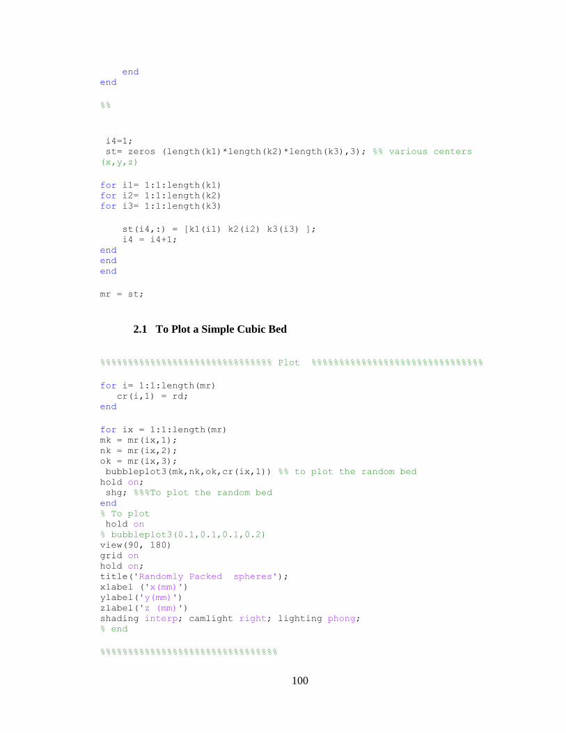
100
end end
%%
i4=1; st= zeros (length(k1)*length(k2)*length(k3),3); %% various centers
(x,y,z)
for i1= 1:1:length(k1) for i2= 1:1:length(k2) for i3= 1:1:length(k3)
st(i4,:) = [k1(i1) k2(i2) k3(i3) ]; i4 = i4+1; end end end
mr = st;
2.1 To Plot a Simple Cubic Bed
%%%%%%%%%%%%%%%%%%%%%%%%%%%%%%% Plot %%%%%%%%%%%%%%%%%%%%%%%%%%%%%%%
for i= 1:1:length(mr) cr(i,1) = rd; end
for ix = 1:1:length(mr) mk = mr(ix,1); nk = mr(ix,2); ok = mr(ix,3); bubbleplot3(mk,nk,ok,cr(ix,1)) %% to plot the random bed hold on; shg; %%%To plot the random bed end % To plot hold on % bubbleplot3(0.1,0.1,0.1,0.2) view(90, 180) grid on hold on; title('Randomly Packed spheres'); xlabel ('x(mm)') ylabel('y(mm)') zlabel('z (mm)') shading interp; camlight right; lighting phong; % end
%%%%%%%%%%%%%%%%%%%%%%%%%%%%%%%%
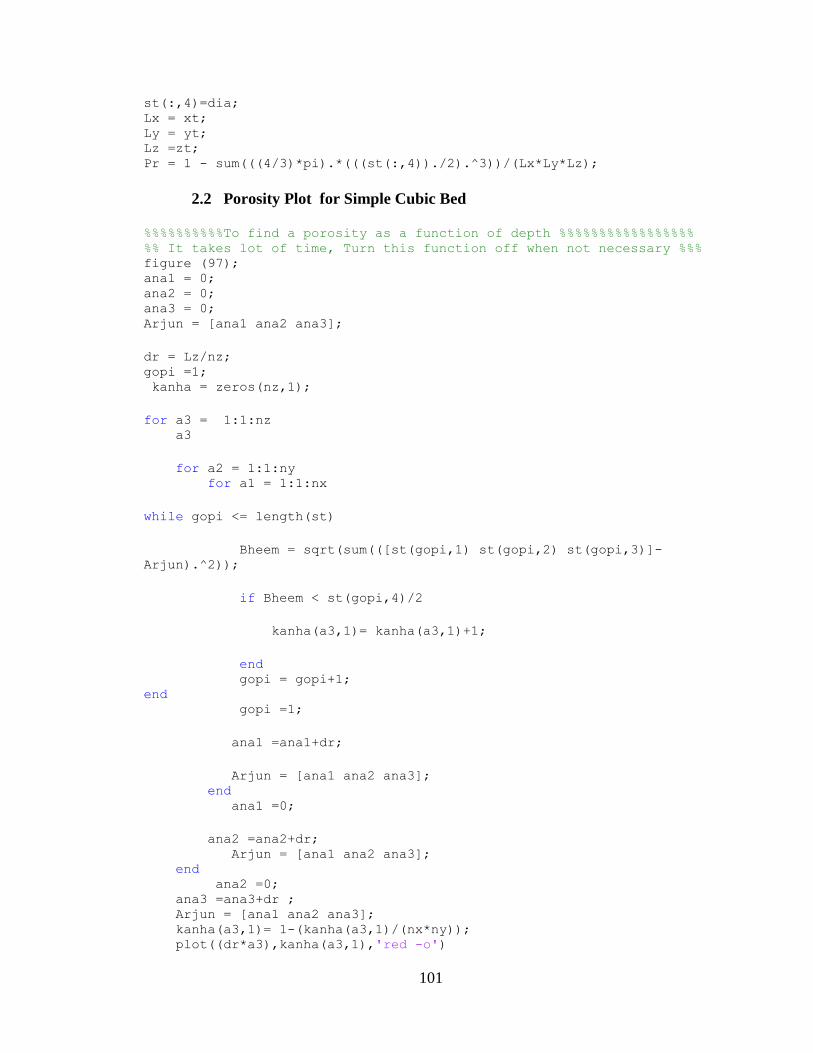
101
st(:,4)=dia; Lx = xt; Ly = yt; Lz =zt; Pr = 1 - sum(((4/3)*pi).*(((st(:,4))./2).^3))/(Lx*Ly*Lz);
2.2 Porosity Plot for Simple Cubic Bed %%%%%%%%%%To find a porosity as a function of depth %%%%%%%%%%%%%%%%% %% It takes lot of time, Turn this function off when not necessary %%% figure (97); ana1 = 0; ana2 = 0; ana3 = 0; Arjun = [ana1 ana2 ana3];
dr = Lz/nz; gopi =1; kanha = zeros(nz,1);
for a3 = 1:1:nz a3
for a2 = 1:1:ny for a1 = 1:1:nx
while gopi <= length(st)
Bheem = sqrt(sum(([st(gopi,1) st(gopi,2) st(gopi,3)]-
Arjun).^2));
if Bheem < st(gopi,4)/2
kanha(a3,1)= kanha(a3,1)+1;
end gopi = gopi+1; end gopi =1;
ana1 =ana1+dr;
Arjun = [ana1 ana2 ana3]; end ana1 =0;
ana2 =ana2+dr; Arjun = [ana1 ana2 ana3]; end ana2 =0; ana3 =ana3+dr ; Arjun = [ana1 ana2 ana3]; kanha(a3,1)= 1-(kanha(a3,1)/(nx*ny)); plot((dr*a3),kanha(a3,1),'red -o')

102
xlabel ('Optical Thickness') ylabel ('Porosity') shg hold on; end
plot((0:1:nz)*dr , kanha); hold on; Pr1 = ones(length(kanha))*Pr; plot((1:1:nz)*dr, Pr1); end
%%%%%%%%%%%%%%%%%%%%%%%%%%%%%%%%%%%%%%%%%%%%%%%%%%%%%%%%%%%%%%%%%%%%%

103
3. MATLAB code for generating a Rhombohydral Packing
function [st,Pr,Lz] = Rhombohydral_Packing(dia,xt,yt,zt,nx,ny,nz) % clc % clear all % close all; % dia = 0.1; % % zt =0.5; % xt =0.5; % yt =0.5; % nx = 100; % ny = 100; % nz = 100;
%%%%%%%%%%%%%%%%%%%%%%%%%%%%%%%%%%%%%%%%%%%%%%%%%%%%%%%% rd = dia/2; k1= [];k2=[]; k3 =[]; % centers of particles st = []; ht = (sqrt(3))*(dia/2);
rx2= dia/2; rx1= dia/2; rx3= dia/2; u5 = 1; o3 =1; while rx3 < zt it3 = rx3;
o2 =1; while rx2< yt it2 = rx2;
if rx2 ==dia/2 guass = 1; elseif rx2 == dia guass =0; end
o1= 1; while rx1 < xt; if rx1 ==dia/2 rieman = 1; elseif rx1 == dia rieman =0; end it1 =rx1;
st(u5,:)=[it1 it2 it3] ; u5=u5+1; rx1 = rx1+dia;
end

104
if rieman ==1 rx1=dia; else rx1 = dia/2; end
rx2= rx2+ht;
end if guass ==1 rx2=dia; else rx2 = dia/2; end
rx3 = rx3+ht;
end
st(:,4)=dia./2; Lx = max(st(:,1))+(dia/2); Ly = max(st(:,2))+(dia/2); Lz = max(st(:,3))+(dia/2); Pr = 1 - sum(((4/3)*pi).*(((st(:,4))).^3))/(Lx*Ly*Lz);
3.1 To Plot a Rhombohydral Bed % figure (50); % for j2 = 1:1:length(st) % m = st(j2,1); % n = st(j2,2); % o = st(j2,3); % l =(st(j2,4)); % bubbleplot3(m,n,o,l) %%%%%%%%%%%% to plot the random bed % shg; %%%%%%%%%%%%%%%%To plot the random bed % end % hold on % % bubbleplot3(0.1,0.1,0.1,0.01) % % view(90, 180) % view (-180,90) % grid on % hold on; % title('Rhombohydral Packing spheres'); % xlabel ('x(mm)') % ylabel('y(mm)') % zlabel('z (mm)') % shading interp; camlight right; lighting phong; % % % to check the porosity of the bed % % Pr = 0.2596; % % end % %%

105
% end % close all
3.2 Porosity Plot for a Rhombohydral Bed % %%%%%%%%%%%To find a porosity as a function of depth
%%%%%%%%%%%%%%%%% % %% It takes lot of time, Turn this function off when not necessary
%%% % figure (97); % ana1 = 0; % ana2 = 0; % ana3 = 0; % Arjun = [ana1 ana2 ana3]; % % dr = Lz/nz; % gopi =1; % kanha = zeros(nz,1); % % for a3 = 1:1:nz % a3 % % for a2 = 1:1:ny % for a1 = 1:1:nx % % while gopi <= length(st) % % Bheem = sqrt(sum(([st(gopi,1) st(gopi,2) st(gopi,3)]-
Arjun).^2)); % % if Bheem < st(gopi,4)/2 % % kanha(a3,1)= kanha(a3,1)+1; % % end % gopi = gopi+1; % end % gopi =1; % % ana1 =ana1+dr; % % Arjun = [ana1 ana2 ana3]; % end % ana1 =0; % % ana2 =ana2+dr; % Arjun = [ana1 ana2 ana3]; % end % ana2 =0; % ana3 =ana3+dr ; % Arjun = [ana1 ana2 ana3]; % kanha(a3,1)= 1-(kanha(a3,1)/(nx*ny)); % plot((dr*a3),kanha(a3,1),'red -o') % xlabel ('Optical Thickness') % ylabel ('Porosity')
106
% shg % hold on; % end % % plot((1:1:nz)*dr , kanha); % hold on; % Pr1 = ones(length(kanha))*Pr; % plot((1:1:nz)*dr, Pr1); end

107
4. MATLAB Code to Create a Gaussian Beam
This function creates a Gaussian beam
function [Z] = Guassianbeam(s_p,s_r,xt,yt,nx,ny)
dx = xt/(nx-1); dy = yt/(ny-1); x0 =xt/2; y0 =yt/2;
sigma_x = 2*s_r; %radius of laser beam. It should always be greater
than min grid size and less than width (xt or yt) sigma_y = 2*s_r; A = s_p; [X,Y] = meshgrid(0:dx:xt, 0:dy:yt);
for theta = 0:(pi/xt):2*pi; a = cos(theta)^2/2/sigma_x^2 + sin(theta)^2/2/sigma_y^2; b = -sin(2*theta)/4/sigma_x^2 + sin(2*theta)/4/sigma_y^2 ; c = sin(theta)^2/2/sigma_x^2 + cos(theta)^2/2/sigma_y^2; Z = A*exp( - (a*(X-x0).^2 + 2*b*(X-x0).*(Y-y0) + c*(Y-y0).^2)) ;
end %% to eliminate the very small numbers in matrix so it's easy to use; for j =1:1:nx for i= 1:1:ny if Z(i,j)<0.01; % 0.01 Z(i,j)=0; end
end end figure(10) surf(X,Y,Z); % shading interp; view(-90,90) hold on; zlabel('Power (W)') title('Guassian Distribution of Laser Beam (100W)') ylabel('y(mm)') xlabel('x(mm)') % view(0,0) end
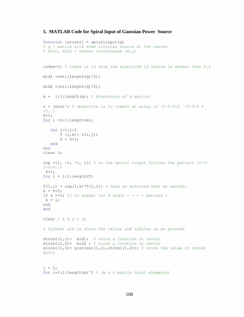
108
5. MATLAB Code for Spiral Input of Gaussian Power Source
function [store1] = spiralinput(q) % q = matrix with some circular source at the center % mid1, mid2 = center coordinates (x,y)
index=1; % index is to stop the algorithm if source is weaker than 0.1
mid1 =ceil(length(q)/2);
mid2 =ceil(length(q)/2);
m = 1:1:length(q); % dimensions of q matrix;
n = [m;m]'; % objective is to create an array of (1-1-2+2 +3-3-4 4
+5..) k=1; for i =1:1:length(m);
for j=1:1:2 T (1,k)= n(i,j); k = k+1; end end clear k;
cop =[1, -1, -1, 1]; % as the spiral output follows the pattern (1-1-
2+2+3..) k=1; for i = 1:1:length(T)
T(1,i) = cop(1,k)*T(1,i); % here we achieved what we wanted. k = k+1; if k ==5; %( to repeat our 4 digit + - - + pattern ) k = 1; end end
clear i k x y n j;
% further aim is store the values and indices as we proceed
store1(1,1)= mid1; % store x location or center store1(1,2)= mid2 ; % store y location or center store1(1,3)= q(store1(1,1),store1(1,2)); % store the value of center
point
j = 1; for i=1:1:length(m)^2 % (m x n matrix total elements)

109
if T(1,i)>0; stop = 1; fk =1; else stop = -1; fk=-1; end
if mod(i,2)==1; % modify y coordinate
while abs(T(1,i))>= abs(stop); mid2 = mid2+fk; store1(j+1,1)= (mid1); % x location store1(j+1,2)= (mid2) ; % y location store1(j+1,3)= q(store1(j+1,1),store1(j+1,2)); j = j+1;
if store1(j,3)<0.1; index = index+1; end
if T(1,i)>0; stop = stop+1; else stop = stop-1; end
end
else % modify x coordinate
while abs(T(1,i))>= abs(stop); mid1 = mid1+fk; store1(j+1,1)=mid1; % x location store1(j+1,2)=mid2; % y location store1(j+1,3)= q(store1(j+1,1),store1(j+1,2));
j= j+1; %% imp conditions
if store1(j,3)<0.1; index = index+1; end
if T(1,i)>0; stop = stop+1; else stop = stop-1 ; end
end

110
end
if index > 6; break; end end end

111
6. Other Functions
%% To convert 3d matrix to 2d function[Ta] = threeDtotwoD(Q1) sz = size(Q1); sz = sz(1,3); for j=1:1:sz Ma= Q1(:,:,j); Ta(j,:)= sum(Ma,1); end end
%% To convert 3d matrix to 1d
function[Ta] = threeDtooneD(Q1) sz = size(Q1); sz = sz(1,3); for j=1:1:sz Ma= Q1(:,:,j); Ta(j,1) = sum(sum(Ma)); end end
%% to store the results in 3d matrix
function [c1,c2,c3] = storephoton(xt,yt,zt,nx,ny,nz,x,y,z)
dx = 0:(xt/(nx-1)):xt; dy = 0:(yt/(ny-1)):yt; dz = 0:(zt/(nz-1)):zt;
for i= 1:1:length(dx) if x <= dx(i); c1= i; break; end end clear i; for i= 1:1:length(dy) if y <= dy(i); c2 = i; break; end end clear i; for i= 1:1:length(dz) if z <= dz(i); c3= i; break;
112
end end clear i end
%% to calculate New angles after reflection %%
function [p,q,r] = New_Angles(Mu_x, Mu_y, Mu_z, Mu, Zai)
if ((sqrt(1-Mu_z^2))> 10^-10)
matrix2 = [Mu_x*Mu_z/(sqrt(1-Mu_z^2)), -Mu_y/(sqrt(1-Mu_z^2)),
Mu_x;Mu_y*Mu_z/(sqrt(1-Mu_z^2)), Mu_x/(sqrt(1-Mu_z^2)), Mu_y;-(sqrt(1-
Mu_z^2)), 0, Mu_z]; [((sqrt(1-Mu^2))*cos(Zai));((sqrt(1-Mu^2))*sin(Zai));Mu]; matrix1 = [((sqrt(1-Mu^2))*cos(Zai));((sqrt(1-Mu^2))*sin(Zai));Mu]; matrix1 = matrix2*matrix1; p = matrix1(1); q = matrix1(2); r = matrix1(3); else
p = ((sqrt(1-Mu^2))*cos(Zai))*sign(Mu_z); r = Mu*sign(Mu_z); q = ((sqrt(1-Mu^2))*sin(Zai))*sign(Mu_z); end end

113
7. Main Code for Radiation Transport in Packed Bed clc; clear all; close all; %% 0 - disable 1 - enable & %%%% others must be 0
dia =0.05; specular =0; diffuse = 1; HG = 0;
RANDOM_BED = 1; %%% Specify d1 & dia RHOMBO_BED = 0; %%% Specify dia CUBIC_BED = 0; %%% Specify dia
Uniform_source = 1; Guassian_source =0;
BED_show = 1; LIVE_PLOT =1; LIVE_PLOT_WITH_NORMAL=0;
%% Optical Properties of Material w = 0.7; %% reflectivity ( default absorbtivity = 1-
reflectivity ) Emissivity = 0; %% ( default absorbtivity = 1-reflectivity ) Rho_surf = 0; %% if 1 all reflection if 0 all absorb
%% BED Dimensions
N =10; % Number of rays zt =0.8; % Depth of the bed in mm (zt+ exon make sure to
acomodate full particle) yt =0.8; % mm; xt =0.8; % mm; ny =100; % Number of grid points in y coordinates nz =100; % Number of grid points in z coordinates nx =100; % Number of grid points in x coordinates
exon =0.00;%(zt/nz); % From Where to start the first layer ? (1
or 2 resolutions)
%% particle Dimensions; % dia =0.5; % mm rd = dia/2; % mm cxy =0.00; %Inter particle clearance in x and y
directions; cz =0.00; % keep it 0 for the realistic purpose. Tr = zeros(nz,1); Trp1 = zeros(nz,1); %% choose type of packing of the bed - (Random/ Uniform / rhombohydral) % Using simple cubic packing then Call particle centers;

114
if CUBIC_BED ==1 && RHOMBO_BED ~=1 && RANDOM_BED ~=1 ; mr = centers_1(dia,nx,ny,nz,xt,yt,zt,cxy,cz,exon); mr = sortrows(mr,3); Porosity =(1-(length(mr)*(4/3)*pi*(rd)^3)/(xt*yt*zt)); for i= 1:1:length(mr) cr(i,1) = rd; end Lz = zt+exon; end %% %%%%%%% if Using Random packing %
if RANDOM_BED ==1; d1 = 0.07; % Small diameter change d1 and d2 for various porosities.
Random d2 = dia; % large diameter keeping d1 = d2 will be problematic ~ random
porosity (0.85)
[mr1,Porosity,Lz] = Randomly_Packied(d2,d1,xt,yt,zt,nx,ny,nz); mr1 = sortrows(mr1,3); mr = [mr1(:,1) mr1(:,2) mr1(:,3)]; cr = mr1(:,4); %%% diameter end
%% %%%%% if Using Random RhombohydralPacking if RHOMBO_BED ==1 && RANDOM_BED ~=1 && CUBIC_BED ~=1; [mr1,Porosity,Lz]= Rhombohydral_Packing(dia,xt,yt,zt,nx,ny,nz); mr1 = sortrows(mr1,3); mr = [mr1(:,1) mr1(:,2) mr1(:,3)]; cr = mr1(:,4); end Porosity
%%%%%%%
%%%%%%%%%%%%%%%%%%%%%%%%%%%%%%%%%%%%% live plot 1 if BED_show ==1 figure (56); grid off for j2 = 1:1:length(mr) m = mr(j2,1); n = mr(j2,2); o = mr(j2,3); l =(cr(j2,1)); bubbleplot3(m,n,o,l) %%%%%%%%%%%% to plot the random bed shg; %%%%%%%%%%%%%%%%To plot the random bed % view(90, 180) % shading interp; % camlight right; lighting phong end shading interp; camlight right; lighting phong hold on; end

115
if LIVE_PLOT ==1 scatter3(0,yt,0,0.001,'o') shg hold on scatter3(xt,yt,zt,0.001,'o') shg % hold on; scatter3(0,0,0,0.001,'o') alpha(0.05) view(180,180) hold on; shg view(120,140) end
% close all; %%%%%%%%%%%%%%%%%%%%%%%%%%%%%%%%%%%%%%%%%%%%%%%%%%%%%%%%%%%%%%%%%%%%%%%
%%%%
%% hold on; LBD1 = (Lz)/dia; % Length to dia ratio
%% define source function s_r =0.04; % Gaussian beam Source Diameter in s_r*10 = mm ; s_p =100; % Watt Source Power (point source) ;
%% Miain code initialize parameters:- [G] = Guassianbeam(s_p,s_r,xt,yt,nx,ny); % creating a Gaussian beam
source Ip = spiralinput(G); % spiral input of Gaussian beam to system; L = length(Ip); Q = zeros(nx,ny,nz); % power matrix for storing power(weights) at any
location x0 =xt/2; % sournce location y0 =yt/2; z0 =0; h =1; Resol = (Lz/nz); Radius_of_particle = rd; if 2*Resol < dia;
%% Miain code:-
h =1; Ni = 0; Nx=0; li = 0; lm = 0; for i = 1:1:N; i
% Source x =xt*(Ip(h,1)/nx); y =yt*((Ip(h,2)/ny)); z =z0; %(location of laser
beam)
116
%% choose type of source (Uniform or Guassian) if Guassian_source==0 && Uniform_source ==1; s_p1 = s_p; % uniform source end if Guassian_source==1 && Uniform_source ==0; s_p1 =Ip(h,3); % Gaussian Source end
Mu_z = 1; % incident angle for the laser beam (1 = 90 deg) phi =2*pi*rand;%0 %isotropic source Source TEMP (0 to 2pi)
Mu_x = sqrt(1-Mu_z^2)*cos(phi); %initial x-direction cosine Mu_y = sqrt(1-Mu_z^2)*sin(phi); %initial y-direction cosine
BTR = 1; o_c =[0 0 0]; n_c =[0 0 0]; P_old = ([x,y,z]');
while BTR >= 1
s = Resol; x = x+s*(Mu_x); y = y+s*(Mu_y); z = z+s*(Mu_z); P = [x y z]; Nx=Nx+1; lm = lm+s;
if LIVE_PLOT ==1; figure(56); scatter3(x,y,z,0.1,'o') shg view(180,180); hold on; end
if 0 <= x && x <= (xt) && 0 <=y && y <= yt && 0 <=z && z <(Lz)
%%%%%%%%%%_ Transmissivity Patch1%%%%%%%%% [x1,x2,x3] = storephoton(xt,yt,Lz,nx,ny,nz,x,y,z); Trp1(x3,1) = Trp1(x3,1)+1; clear x1 x2 x3; %%%%%%%%%%
i1 =1; j1=1; %% j1 = 1 check while i1 < length(mr) % to check the location of closest center
test = sqrt(sum(([mr(i1,:)- P]).^2)); % distance from the
closest center
117
if test <= (cr(i1,1)) j1 =i1;
i1= length(mr)+1; n_c = mr(j1,:);
else test=10; n_c =[0 0 0]; end i1= i1+1;
end
if sum(o_c-n_c)~=0; %%%% checking for same center not ? o_c = n_c;
if test <= (cr(j1,1)) ;
god = cr(j1,1)-test; god1 = god*(Mu_x); god2 = god*(Mu_y); god3 = god*(Mu_z);
x = x-god1; y = y-god2; z = z-god3;
Ni=Ni+1; li=li+s; %% %%%%% sys1 [x1,x2,x3] = storephoton(xt,yt,Lz,nx,ny,nz,x,y,z); Q(x1,x2,x3)= Q(x1,x2,x3)+(1-w)*s_p1; % absorbed energy
during the process; s_p1 = w*s_p1; %% remaining energy Tr(x3,1) = Tr(x3,1)+1; % % %%% sys2 % riemann =rand; % if riemann >= w % [x1,x2,x3] = storephoton(xt,yt,Lz,nx,ny,nz,x,y,z); % Q(x1,x2,x3)= Q(x1,x2,x3)+s_p1; %absorbed energy
during the process; % s_p1 = 0; %% remaining energy % Tr(x3,1) = Tr(x3,1)+1 ; % end % % %%% sys3 % %%%%%%%%%%%%%%%%%%%%%%%%%%%%%%%%%%% with emission effect % riemann =rand; % if riemann > w %% reflect % [x1,x2,x3] = storephoton(xt,yt,Lz,nx,ny,nz,x,y,z);

118
% Q(x1,x2,x3)= Q(x1,x2,x3)+(1-Emissivity)*s_p1; %
absorbed energy during the process; % s_p1 = Emissivity*s_p1; %% emission; % Tr(x3,1) = Tr(x3,1)+1; % end %%%%%%%%%%%%%%%%%%%%%%%%########### live plot2 if LIVE_PLOT ==1; figure(56) scatter3(x,y,z,10,'o') view(180,180); shg; hold on; end
%%%%%%%%%%%%%%%%%%%%%%%%%%%%%%%%%%%%%%%%%%%%
%% Choose type of reflection (Diffused/ specular or isotropic
scattering)
%%%%%%%%%%%%%%%%############### FOR Specular Reflectrion if specular == 1 && diffuse ==0 && HG ==0;
if s_p1 ~=0; syms xu yu zu ; Vn1 = (xu-mr(j1,1))^2+(yu-(mr(j1,2)))^2+(zu-
mr(j1,3))^2-(cr(j1,1))^2; Gr_Vn1 = gradient(Vn1, [xu,yu,zu]); Gr_Vn1= subs(Gr_Vn1,{xu,yu,zu},[x,y,z]); eval (Gr_Vn1); Mag_Vn1 = sqrt((Gr_Vn1(1,1))^2+ (Gr_Vn1(2,1))^2+
(Gr_Vn1(3,1))^2); Mag_Vn1 = eval(Mag_Vn1); normal1 = Gr_Vn1/Mag_Vn1; normal1 = eval(normal1); %% Unit normal vector Pr = sqrt(sum((P_old-[x;y;z]).^2)); %% To find
angle between unit normal and incoming vector Nr= sqrt(sum((normal1).^2)); clear xu yu zu Vn1 Gr_Vn1 Mag_Vn1; Bet = acos((sum((normal1).*(P_old-
[x;y;z])))/(Pr*Nr)); %% Specular reflection
% % % Bet =
atan2(norm(cross(normal1,P_old)),dot(normal1,P_old));
Mu = cos(pi-2*Bet); phi = 2*pi*rand; z_old = P_old(3,1); if (x - mr(j1,1))< 0 %%% backward hemisphere if z_old > z %% top hem Zai = rand*(pi);% 0; else %% bottom hem Zai = pi+(rand*(pi)); end else %%% Forward hemisphere

119
if z_old > z %% top hem Zai = pi+(rand*(pi)); else %% top hem Zai = rand*(pi); %%%0; end end [Mu_x,Mu_y,Mu_z]=
New_Angles(Mu_x,Mu_y,Mu_z,Mu,Zai);
%%%%%%%%%%%%%%%%% live plot-1 %% to Plot the surface normal from
the spheres if LIVE_PLOT_WITH_NORMAL ==1 figure (56) uc1=normal1(1,1); uc2=normal1(2,1); uc3=normal1(3,1); quiver3 (x,y,z,uc1,uc2,uc3,0.5); hold on; end %%%%%%%%%%%%%%%%%%%%
Ursa =1; king=1; leo = [Mu_x Mu_y Mu_z]; while Ursa == 1 ; %% to make sure that photon doesnt penetrate the
sphere
n_p = [x+Resol*(Mu_x) y+Resol*(Mu_y)
z+Resol*(Mu_z)]; pax = sqrt(sum(([mr(j1,:)-n_p]).^2)); if pax < cr(j1,1) %% going again in same
sphere king=king+1; %%% Mu will remain the same Zai = 2*pi*rand; Mu_x = leo(1,1); %%setting the original
value Mu_y = leo(1,2); Mu_z = leo(1,3);
[Mu_x,Mu_y,Mu_z]=New_Angles(Mu_x,Mu_y,Mu_z,Mu,Zai);
else Ursa =0;
end if king ==5000; Ursa = 0; s_p1=0; end end end
%%%%%%%%%%%%%%%%%%%%%%%%% Imp %% don't disable
%%%%%%%%%%%%%%%%%%%%%%%%%%%

120
P_old = ([x,y,z]'); %%%%%% imp %% don't disable end
%%%%%%%%%%%%%%%%%%%% Specular REflcetion ends
%%%%%%%%%%%%%%%%%%%%%%%%%% %% if specular == 0 && diffuse ==0 && HG ==1; %%%%%%%%%%%%%%%%%%%%%####### Small particles ALL TYPE OF SCATTERING
USING GREENSTIN Function % % g = +0.01;%%%%%-0.7 for diffused backscattering; Mu =(1+g^2-((1-g^2)./(1+g-2*g*rand)).^2)./(2*g); x= mr(j1,1); y= mr(j1,2); z =mr(j1,3);
Zai = 2*pi*rand; [Mu_x,Mu_y,Mu_z]=New_Angles(Mu_x,Mu_y,Mu_z,Mu,Zai);
%%%%%%%%%%%%%%%%%%%%%%%%% imp %% dont disable
%%%%%%%%%%%%%%%%%%%%%%%%%%% P_old = ([x,y,z]'); %%%%%% imp %% don't disable end %% %%%%%%%%%%%%%%%%%%%%%%%%%%%%%%%%% FOR DIFFUSE REFLECTION if specular == 0 && diffuse ==1 && HG ==0; Zai = 2*pi*rand; Mu = 1-2*rand; %Isotopic scattering.
[Mu_x,Mu_y,Mu_z]=New_Angles(Mu_x,Mu_y,Mu_z,Mu,Zai); %new direction
Ursa =1; king=1; leo = [Mu_x Mu_y Mu_z]; while Ursa == 1 %%% Ursa will take care that the photon will not go
into particle
n_p = [x+Resol*(Mu_x) y+Resol*(Mu_y)
z+Resol*(Mu_z)]; pax = sqrt(sum(([mr(j1,:)-n_p]).^2)); if pax < cr(j1,1) %% going again in same
sphere king=king+1; Mu = 1-2*rand; Zai = 2*pi*rand; Mu_x = leo(1,1); %%setting the original
value Mu_y = leo(1,2); Mu_z = leo(1,3);
[Mu_x,Mu_y,Mu_z]=New_Angles(Mu_x,Mu_y,Mu_z,Mu,Zai);
else Ursa =0;

121
end if king ==5000; Ursa = 0; s_p1=0; end end end %%%%%%%%%%%%%%%%%%%%%%%%%%%DIFFUDE REFLECTION ENDS HERE
%%%%%%%%%%%%%%%%%%%%%%%%%%%%%%%%%%%%%%%
end end
%%%%%%%%%%%%%%%%%%%%%%%%%%%%%%%%%%%%%%%% FOR Periodic Boundary boundary elseif x <0 && 0 <=y && y <= yt && 0 <=z && z <(Lz) ; x = xt; P_old = ([x,y,z]'); elseif x > (xt) && 0 <=y && y <= yt && 0 <=z && z <(Lz) ; x = 0; P_old = ([x,y,z]'); elseif 0 <= x && x <= (xt) && 0 < y && 0 <=z && z <(Lz) ; y = yt; P_old = ([x,y,z]'); elseif 0 <= x && x <= (xt) && y > yt && 0 <=z && z <(Lz) ; y = 0; P_old = ([x,y,z]'); %%%%%%%%%%%%%%%%%%%%%%%%%%%%%%%%%%%%%%%%%%%%%%%%%%%%%%%%%%%%%
elseif 0 <= x && x <= (xt) && 0 <=y && y <= yt && z >= (Lz) %%%
&& z <=(Lz)
z = Lz; %%%%%%%%%%%%%%%%%%%%%%%%%%%%%%%%%%%% live plot 2; % figure(56) % scatter3(x,y,z,10,'o','red') % view(180,180); % shg; % hold on; %%%%%%%%%%%%%%%%%%%%%%%%%%%%%%%%%%%%%%%%%%%%%%%%% [x1,x2,x3] = storephoton(xt,yt,Lz,nx,ny,nz,x,y,z); Q(x1,x2,x3)= Q(x1,x2,x3)+(1-Rho_surf)*s_p1; %
absorbed energy during the process; Tr(x3,1) = Tr(x3,1)+1;
s_p1 = Rho_surf*s_p1; %% remaining energy
Mu = -sqrt(rand); %Lambertian reflection. Zai = 2*pi*rand;%isotopic scattering [Mu_x,Mu_y,Mu_z]=New_Angles(Mu_x,Mu_y,Mu_z,Mu,Zai);
denabola = 1; Queen = 1; while denabola ==1 && s_p1~=0; Queen =Queen +1;

122
springfield = z+Mu_z*s;
if springfield > Lz
Mu = -sqrt(rand); %Lambertian reflection. Zai = 2*pi*rand;%isotopic scattering [Mu_x,Mu_y,Mu_z]=New_Angles(Mu_x,Mu_y,Mu_z,Mu,Zai);
else denabola = 0; end if Queen> 5000; denabola= 1; s_p1=0; end end if s_p1< 0.001 BTR =0; end
%% %%%%%%%%%%%%%%%%% %%%%%%%%%%%%%%%%%% Dont disable P_old = ([x,y,z]'); %%%%%%%%%%%%%%%%%%%%%%%%%%%%%%%%%% else BTR =0; end
if s_p1< 0.001 BTR =0; end end
h = h+1; if L < (h) h=1; end
end %% else 'diameter of the particle (rd)is too small for resolution.(d)' break; end
Ext_coef =(Ni/Nx)/s Non_ext = Ext_coef*dia
% % % % % % % % clearvars -except Q N d resolution xt yt zt; Q1 =(Q/(N)); % normalize; check = max(max(max(Q1)));
123
%%%For 1D plot hold on;
[T1] = threeDtooneD(Q1); base_e = T1(end) T1(end)=0; check =(max(T1));
T1 =(T1./(check)); dz = 0:((Lz)/(nz-1)):(Lz); LBD = 0:((LBD1)/(nz-1)):LBD1; % sd = (LBD1/nz): (LBD1/nz):LBD1;
%% %%%%%%%%%%% Plot For Transmissivity % % Layers = 32; %% number of effective layers in the bed; z_ind = ((1.5*(1-Porosity))/ ((1-Porosity)/0.524)^(1/3))*Layers; dz2 = 0:((z_ind)/(nz-1)):z_ind;
% crv = 0;%Tr(end); % Tr1 = Tr/(N); Tr1(end)=0; Tr1 = Tr1/max(Tr1); % % Tr1 = Tr1./sd'; % %%%%%%%%%%%%%%%%%%%%%%%%%%%% % Trp2 = (Trp1)-crv; % Trp2 = Trp2/(N); % Trp2 = Trp2/max(Trp2); % % % Trp2 = Trp2./sd'; %%%%%%%%%%%%%%%%%%%%%%%%%%%% close all; % sparton2() hold on semilogy(dz2,Trp2./dz2','-b*'); hold on; semilogy(dz2,Tr1./dz2','-g*'); grid on; hold on;
%%%%%%%%%%%%%%%%%%%%%%%%%Flor for %%%%%%%%%%%%%%%%%%%%%%%%%%%%%%% Tr2 = Tr1.*sd'; Tr2 = Tr1(1:end-15);%Tr1(5:end-15) sd2 = sd(1:end-15); %Tr1(5:end-15) % sparton(Tr2,sd2,dz2); % Validaton cases % sparton(Tr1,sd,dz2) % Validaton cases xlabel('Tau_ind'); ylabel('Nondimensional Energy flux') title('Effect of Particle size') figure (20); plot (dz,T1','blue') %%%%%%%%%%%%%%%%%%%%%%%%%%%%%%%%%%%%%%%%%%%%%%%%%%%%%%%%%%%%%
%%

124
% % % % % % % % For 2D Plot. figure(21) clear i j1 j2 ; [T] = threeDtotwoD(Q1); T =(T./(check));
[X1,Z1] = meshgrid( 0:(xt/(nx-1)):xt,0:(Lz/(nz-1)):Lz); subplot(2,2,1) surf (X1,Z1, T); view(320,-235); %% 3d view; shading interp; % colorbar() ylabel('Optical thickness z(mm)') xlabel('width x(mm)'); zlabel('Absorbed Energy/Toal Energy (E/Etotal)')
subplot(2,2,4) surf(X1,Z1, T); view(360,180) %% Side view; % shading interp; ylabel('Optical thickness z(mm))') xlabel('width x(mm)'); zlabel('Absorbed Energy/Toal Energy (E/Etotal)')
subplot(2,2,2) surf (X1,Z1, T); view(-360,270); %% top view; ylabel('Optical thickness z(mm)') xlabel('width x(mm)'); zlabel('Absorbed Energy/Toal Energy (E/Etotal)') % colorbar() % shading interp; hold on; title ('Angle of Incidence = 66 deg ')
subplot(2,2,3) surf (X1,Z1, T); view(90,360) ylabel('Optical thickness z(mm)') xlabel('width x(mm)'); zlabel('Absorbed Energy/Toal Energy (E/Etotal)') shading interp;
% %%%%%%%%%%%%%%%%%%%%% others %%%%%%%%%%%%%%%%%%%%%%%%%%%%%%
% To plot the Y cross section hold on; Y_cross(Q1,xt,zt,nx,nz,50); %% (at y = 50) hold on;
%%%%%%%%%%%%%%%%%%%%%%%%%%%%%%%%%%%%%%%%%%%%%%%%%%%%%%%%%%%%%%%%%%%%%%%
%%%%%
125
%% FOR 3d Plot % % % % % % clearvars -except Q xt yt zt ; % figure(22); % % u = size (Q); % u1 = u(1,1); % u2 = u(1,2); % u3 = u(1,3); % % v1 = xt/u1; % v2 = yt/u2; % v3 = zt/u3; % % M = max(max(max(Q))); % % % for m1 = 1:1:u1 % for m2= 1:1:u3 % for m3 = 1:1:u2 % Mk= (Q(m1,m2,m3)/M); % if Mk > 0.1 % % % %% for red shading %
scatter3((m1*v1),(m2*v2),(m3*v3),Q(m1,m2,m3),...%'s','filled',... % 'MarkerFaceColor',[(Mk) 0 0],'MarkeredgeColor',[(Mk) 0
0] ) % set(gca,'Color',[1 1 1]) % hold on; % shg; % end % [m1 m2 m3] % end % end % % % % shading interp; % end % xlabel(' x(mm)'); % ylabel('y(mm)'); % zlabel('z(mm)'); % colorbar(off); % view(-90,360) % for the top view % view(270,90) % for the side view % % % % % % % In scatter plot % % scatter3(x1,x2,x3,s_p1,'.') % % set(gca,'Color',[0 0 0]) % % grid on; % % shg; % % hold on
%%%%%%%%%%%%%%%%%%%%%%%%%%%%%%%%%%%%%%%%%%%%%%%%%%%%%%%%%%%%%%%%%%%%%%%
%%%
save Transm_check1.mat Q1 T1 Tr Ni Nx li lm s Porosity Lz dia LBD1 dz2
cxy mr cz dz s_r w xt yt zt exon N

126
VITA
Manish B. Patil was born in Mumbai, India on October 1986. He received his diploma
in Mechanical Engineering from SBM polytechnic, and pursued his bachelor's degree in
Mechanical Engineering from the University of Mumbai in June 2009. After his
graduation he joined C-met engineering India Ltd. as a hydraulic engineer. Later on in
December 2011, he worked with Eirich India Ltd. In order to learn advance techniques
in fluid mechanics and heat transfer, he decided to pursue Master of Science degree. He
joined mechanical engineering department at LSU in Fall 2012. During his master's at
LSU, he also worked as a graduate research and teaching assistant. He organized and co-
chaired the 16th
annual Mechanical Engineering graduate student conference in Spring
2016. He expects to receive his master’s degree in Mechanical Engineering in May 2016.