radiation models in fixed beds

Radiation Models in Fixed Beds

A Major Qualifying Project Report

Submitted to the Faculty of the

Worcester Polytechnic Institute

In partial fulfillment of the major requirements for the

Degree of Bachelor of Science in Chemical Engineering

By

Nathan Caso

Project Advisor

Anthony Dixon

April 2017

1

Table of Contents Abstract ......................................................................................................................................................... 3

Chapter 1: Introduction ................................................................................................................................ 4

Chapter 2: Background ................................................................................................................................. 6

2.1 – ANSYS Fluent .................................................................................................................................... 6

2.1.1 – Fluent Radiation Models ........................................................................................................... 6

2.1.2 – Discrete Ordinates .................................................................................................................... 6

2.1.3 – Surface to Surface Radiation ..................................................................................................... 7

2.1.4 – Under Relaxation....................................................................................................................... 9

2.2 ‐ Models of Effective Thermal Conductivity ........................................................................................ 9

2.2.1 – Zehner Schlünder (ZS) Model .................................................................................................. 10

2.2.2 – Zehner Bauer Schlünder (ZBS) Model ..................................................................................... 10

2.2.3 – Gaps......................................................................................................................................... 12

2.2.3 – Breitbach‐Barthels (BB) Radiation method ............................................................................. 12

2.2.4 – Sih‐Barlow (SB) Method: ......................................................................................................... 13

2.2.5 – Damköhler Equation ............................................................................................................... 13

2.3 – Modeling the Near Wall Effect ....................................................................................................... 13

2.3.1 – Tsotsas Modification ............................................................................................................... 14

Chapter 3: Methodology ............................................................................................................................. 15

3.1 – Fluent Models ................................................................................................................................ 15

3.1.1 – Setup ....................................................................................................................................... 15

3.1.2 Calculation ................................................................................................................................. 18

3.1.3 Extraction of Results .................................................................................................................. 18

3.2 – COMSOL Models ............................................................................................................................ 18

3.2.1 – NWE Modeling ........................................................................................................................ 19

3.2.3 – General Considerations ........................................................................................................... 19

Chapter 4: Results and Discussion .............................................................................................................. 22

4.1 – Discrete Ordinates versus Surface to Surface radiation ................................................................ 22

4.2 – Effect of Gaps ................................................................................................................................. 23

4.3 – Effect of Radiation .......................................................................................................................... 23

4.4 – ZBS versus CFD ............................................................................................................................... 24

4.5 – Zehner Schlünder versus CFD......................................................................................................... 26

4.6 – Sih‐Barlow versus CFD .................................................................................................................... 27

2

4.7 – Near Wall Effect ............................................................................................................................. 28

Chapter 5 – Conclusions and Recommendations ....................................................................................... 31

Chapter 6 – References ............................................................................................................................... 32

Chapter 7 – Appendices .............................................................................................................................. 33

Appendix A ‐ Variables list, N=4.5 ........................................................................................................... 33

Appendix B ‐ Parameters List, N=4.5 ...................................................................................................... 33

Appendix C – Void Fraction Data ............................................................................................................ 34

Appendix D – Interpolation Function values – N=4.5 ............................................................................... 1

Appendix E – Expanded Comparisons for N=3.5, 5.5, 6.5 ......................................................................... 2

3

Abstract

Modeling heat transfer in packed beds, important for process optimization and safety control, has been

done for conduction and convection with both the effective thermal conductivity method from

literature and computational fluid dynamics (CFD). This project adds radiation as a heat transfer mode

into both approaches. CFD simulations and literature equations were compared varying the model for

radiation, mitigating the near wall effect, and varying the effective thermal conductivity model. It was

found that one combination of literature methods accurately matches the results of the CFD

simulations, indicating that the effective thermal conductivity model, controlling for the near wall effect,

and using the Damköhler radiation model accurately predicts heat transfer behavior in packed beds.

4

Chapter 1: Introduction

Many important industrial chemical production processes including heating, cooling, drying, catalytic

reactions, and absorbers require knowledge of how heat is transferred in solid‐particle ‐ fluid mixtures.

Heat, mass transfer, and catalytic reaction rates are all proportional to surface area, which is often

maximized in unit operations by using a cylindrical tube filled with small particles, often referred to as a

“packed‐bed”, through which a fluid passes or remains stagnant in the case of a “fixed” bed. Industry,

government, and academia have invested resources into modeling temperature gradient behavior in

such particle beds to improve efficiency and prevent damage resulting from poor temperature control,

such as in the case of a runaway reaction (DiNino et al, 2013).

The late 20th and early 21st century saw increased awareness and understanding of one particular

modeling approach: effective thermal conductivity. The theory behind this method involves using the

measurable or predictable quantity of void fraction to calculate an all‐encompassing thermal

conductivity among multiple heat transfer modes as if a homogeneous mixture with a thermal

conductivity varying by radial position replaced the actual particles in the bed. The temperature gradient

generated by this approach also depends on the thermal conductivities of the fluid and solid particles,

surface emissivities, the absorption coefficient of the fluid, particle shape, and the area of surface

contact among particles. Effective thermal conductivity is inclusive of both stagnant conduction and

radiation as well as convective heat transfer with a moving fluid, but the scope of this project only

includes fixed beds with a non‐moving fluid medium. Proposed by Hengst in 1933, refined in a Chemical

Engineering context by Kunii and Smith in 1960, and improved and empirically verified in the 1970’s by

Schlünder and Zehner (1972), and Bauer (1978) (ZBS used further in this document refers to the works

of Zehner, Bauer, and Schlünder), this approach was shown to be effective at modeling temperature

gradients in stagnant packed beds.

There are several holes in the theory, however, including the near‐wall region predicament. In a packed

bed, particles are largely randomized in the center core region, but as one approaches the wall

boundary of the bed, the particles become geometrically organized resulting in an increase in void

fraction directly next to the wall. The result is a drop in thermal conductivity due to the dominance of

conduction through the fluid rather than solid to solid conduction (Thurgood et al., 2004). This effect is

particularly pronounced in beds of low tube to particle diameter ratio (notated as N in this study). ZBS’s

correlations do not realistically correlate void fraction to the expected change in thermal conductivity,

and binary‐region methods, such as that proposed by Tsotsas (2002), can introduce a non‐physical jump

in thermal conductivity in the transition from core to near‐wall regions.

Entering the 21st century and the digital revolution, a myriad of new technology‐based engineering tools

have become available. Computational Fluid Dynamics (CFD) software originally developed for

aeronautical and military applications based on the Finite Volume Method has become available for

widespread use, and Finite Element Method packages originally used for civil engineering have also

become common. Processing power has also dramatically increased, suggesting the feasibility of using

software to model engineering problems such as the aforementioned temperature gradients in packed

beds. The focus of this project will be on Resolved Particle CFD, instead of the effective medium

5

approach from conventional CFD. A project by Gurnon (2013) suggested that for N=4, CFD modeling

produces similar results to the effective thermal conductivity models developed by Zehner, Bauer, and

Schlünder for at least conduction through the fluid and between particles, neglecting radiation and

surface area contact.

The objective of this project is to extend past research by comparing radiation models in CFD to the

effective thermal conductivity model equations including radiation. ANSYS’s Fluent 16.2 CFD software

was used to simulate both radiative and conductive heat transfer in several 3‐dimensional annular

packed bed models of varying particle diameter to cylinder diameter ratio. COMSOL Multiphysics was

used to generate one‐dimensional temperature profiles based on models found in literature. Assuming

that CFD is accurate, the objective of this project is to draw conclusions about the models from

literature, and to find a combination of them that matches CFD.

6

Chapter 2: Background

2.1 – ANSYS Fluent

Fluent is ANSYS's computational fluid dynamics solver. It uses finite volume analysis to approximate

differential equation problems given boundary conditions. Fluent works by successively iterating

differential approximations among thousands of cells in a mesh until a parameter (in this study the net

heat transfer rate from the outer wall of an annular tube and the annular wall) desirably approaches

zero.

Fluent offers two processing modes: serial and parallel. Serial mode operates with one processor

running, and parallel mode allows the user to select the number of computer processors for use for

more computational power and faster calculations. Fluent also offers a double precision solver option

for higher accuracy in results at the expense of computational load.

2.1.1 – Fluent Radiation Models

Two radiation models were used in Fluent to generate temperature profiles: Discrete Ordinates (DO),

and the Surface to Surface (S2S) method (ANSYS Academic Research, Release 16.2).

2.1.2 – Discrete Ordinates

To understand Discrete Ordinates, one must understand the Radiative Transfer Equation (RTE):

→,→→,→

4→,→ ′ Ф → ∙→ ′

(1)

Table 1: RTE Parameters

→ Position vector

→ Direction Vector

→' Scattering direction vector

s Path Length

a Absorption Coefficient

n Refractive Index

7

σs Scattering Coefficient

σ Stefan‐Boltzmann Constant

I Radiation Intensity, a function of the position and direction

T Local Temperature

Ф Phase function

Ω’ Solid Angle

From the equation, in a small slice of distance, the change in intensity of radiation as a function of

position and direction depends term by term on absorption by a medium due to its “optical thickness”

or opacity, emission by the medium driven by its temperature, and scattering by the medium.

Discrete Ordinates takes this equation and solves it for a finite number of discrete angles associated

with a vector direction, →, in the Cartesian coordinate system. The RTE is transformed into a field

equation and solved as such:

∙ →,→ ,→ →,→

4→,→ ′ Ф → ∙→ ′

(2)

The user controls the number of directions by the fineness of the angular discretization with the

parameters Theta/Phi divisions and pixels. Increasing the value of these parameters increases the

number of transport equations that the model solves for, making the solution more accurate at the cost

of computational load.

Fluent offers several advanced options for calculation, such as Energy/DO Coupling, Non‐Gray model

bands, and semi‐transparent walls. These features were not used in this study so as to be consistent

with the assumptions in the second radiation method, S2S, explained below.

2.1.3 – Surface to Surface Radiation

The S2S model uses mesh‐dependent geometric view factors to account for radiative heat transfer in a

system. This model assumes all surfaces are gray and diffuse, meaning that surface properties are

independent of radiation wavelength and incident angle. Absorption, emission, and scattering by the

medium are also ignored. The equation is derived from a simple energy balance, assuming that

emissivity is equal to absorptivity, and that surfaces are opaque such that only reflection and

transmission are considered:

, ,

(3)

8

Table 2: Radiation Energy Balance

qk,out Energy flux out from surface k

εk Emissivity of surface k


T Temperature of surface k

ρ Fraction of incident flux that is reflected

qk,in Energy flux incident on surface k from its surroundings

In the last term in this equation, the energy incident on surface is dependent on the view factor

between and its surrounding surfaces, . The total flux is put in terms of the energy leaving all other

surfaces that are “visible” to surface :

, ,

(4)

Where is the corresponding area of surface or , and is the view factor between surfaces and .

Using the reciprocity of view factors (AjFjk = AkFkj) and substituting back into Equation 3, the radiosity of

surface is expressed as a function of the emissive power of surface ( and the radiosity

of other surfaces in N equations:

(5)

Which is of the Matrix equation form KJ = E, where K is an N x N matrix, J is the radiosity vector, and E is

the emissive power vector.

Iterating S2S model calculations is intended to take less time than other models such as Discrete

Ordinates. The drawback, however, is that prior to iterations, one must calculate all the view factors

between every surface. Fluent does this with the equation:

1

(6)

Where δij is equal to 0 if the surfaces are not “visible” to each‐other, and 1 if they are. To determine

what surfaces are visible to other surfaces, the Ray Tracing method is used, which follows a ray fired

9

from the center of each surface or face to determine which other surfaces are directly touched, and thus

are “visible”.

Fluent additionally allows users to “cluster” radiating surfaces should one want to decrease the

computational load of a calculation. This algorithm simply takes several faces and treats them as if they

were a single face. Increasing the value reduces the memory load of the view factor file at the cost of

some accuracy. The default setting of using the base faces with no clustering was used for this project.

2.1.4 – Under Relaxation

Under Relaxation factors allow for stabilization of iterative results by minimizing oscillations per the

following equation:

1

(7)

Table 3: Under Relaxation Equation Parameters

Sf Source to Flow

Sp Source from Particles

Uf Under Relaxation Factor

By under‐relaxing particle source terms, the probability of oscillating iterations or divergence is

decreased, at the cost of a more iterations being required to reach an accurate result.

2.2 ‐ Models of Effective Thermal Conductivity

The “so‐called” or effective thermal conductivity, , is an interpretation of thermal conductivity from

Fourier’s law, specifically for cylindrical packed beds. It is derived from the transient equation describing

heat transfer in a packed bed, in terms of radius :

1

1

Table 4: Radial Heat Transfer Energy Balance Parameters

(8)

qr Radial Heat flux at radius r

Bed porosity

ρs, ρg Density of solid and gas

cp, cg Heat capacity of solid and gas

10

Fourier’s law states that the heat flux in a system is proportional to its thermal conductivity. In the case

of a packed bed, the “so‐called” or effective thermal conductivity represents the conductivity of the

stagnant particle/gas mixture as if it were a homogeneous substance. It lumps the fluid/solid conduction

terms as well as radiation into a single term dependent on radial position and bed properties:

(9)

It is crucial to note that is a function of radial position. The encompassment of all heat transfer

modes makes it possible to solve or approximate the heat balance equation given boundary conditions,

thus providing a way to approximate temperature profiles and predict bed behavior. There are several

models in the literature that have been used to do this:

2.2.1 – Zehner Schlünder (ZS) Model

Zehner and Schlünder (1972) modeled effective thermal conductivity by considering a unit cell between

two adjacent particles, and used thermal resistance theory coupled with empirical correlations to define

effective thermal conductivity as such:

1 √1

2√1

1

1

1ln

1 12

1

1

(10)

Table 5: ZS Equation Parameters

λso Effective/so called thermal conductivity

λf Fluid medium thermal conductivity

λs Solid particle thermal conductivity

Bed porosity

B Deformation parameter

The deformation parameter depends on the void fraction, and was empirically defined in ZS’s paper:

1.251

(11)

The ZS model does not account for radiation, but serves as a baseline comparison to the latter models in

which radiation was added.

2.2.2 – Zehner Bauer Schlünder (ZBS) Model

11

Bauer and Schlünder (1978) improved on the previous ZS model by adding radiation, considering the

Knudsen regime/Smoluchowski effect, and adding a parameter for surface contact fraction. The

resulting equation is:

1 √11

√1∗

1∗

(12)

Where

∗ 2

∗1 ∗

∗

1 1∗

1

12

1 1

(13)

And

1 ∗ 1 1 ∗

(14)

Table 6: ZBS Equation Parameters

λD Gaseous thermal conductivity by the Smoluchowski effect

λr Thermal conductivity radiation parameter

λs* A parameter for increased surface area due to metallic oxidation. Equal to λs when the particles

are not metallic.

ϕ A parameter that allows for additional heat transfer through the solid path between contiguous

particles.

For the ZBS model, the radiation conductivity expression is as follows:

421

Table 7: ZBS Radiation Conductivity Parameters

(15)


Emissivity

Particle Diameter

12

T Local Temperature

It was made known by professor Anthony Dixon through private communication that λD had a negligible

effect on models of the geometry used in this study; therefore, this parameter was set to 1 and ignored

when the equation was solved. λS* was assumed to be equal to λS for this study.

2.2.3 – Gaps

To mimic the dimensions of the actual mesh that was used in Fluent, which included a small gap

between particles, an equation was derived using thermal resistance theory that added a small gap of

length 2 into the unit cell system, through which only fluid conduction and radiation heat transfer

occur. The derivation with gaps adds a second system in series to the normal unit particle cell circuitry to

account for the gap:

Figure 1: Circuitry Diagram for the Gaps Equation Derivation

The resulting equation for the effective thermal conductivity with gaps was found to be:

21 √1 ∗ √1 ∗

2

(16)

Where the term is half of the gap distance between two particles.

2.2.3 – Breitbach‐Barthels (BB) Radiation method

To compare the ZBS method to another model of radiation, Breitbach and Barthels’ (1990) factor for

radiation was explored. This “Factor”, , is another way of expressing λR:

4 (17)

In the case of BB radiation, is defined as such:

13

1 √1

√12

1

1 1

11

2 1

(18)

Where:

4

(19)

2.2.4 – Sih‐Barlow (SB) Method:

Sih and Barlow (1994) re‐derived the formula originally proposed by Zehner and Schlünder, and noted

that some mistakes had been found. Their resulting equation for λSO is as follows:

1 √1 1

√1 12

1 1

1 ln1

21

1

(20)

2.2.5 – Damköhler Equation

Sih and Barlow used yet another definition of λR, defined by Damköhler (1937):

4 (21)

Table 8: Damköhler Equation Parameters

F View Factor, approximately 1/3 according to

Damköhler


T Temperature

xR Effective length between particles (in meters), the

same as the particle diameter

2.3 – Modeling the Near Wall Effect

14

Thurgood et al (2004) demonstrated a problem with the ZS and ZBS models. In the near wall region,

defined by Thurgood as the region within one particle’s radius distance from a column wall, the void

fraction approaches one due to a more conformed arrangement and shape of the particles. It is

expected that the effective thermal conductivity approaches the thermal conductivity of the fluid.

However, according to the ZBS model, λso runs off to infinity, which does not accurately represent the

physical reality of the system. This happens because of the term √1 appearing in the denominator

of the “P” function in Equation 14.

2.3.1 – Tsotsas Modification

Tsotsas (2002) came up with a near wall region correction that can be used in a piecewise function. This

allows for one to define the effective thermal conductivity for the near wall region differently from the

core regions:

1 √1 √11

(21)

Where λ0 is equal to λso with λR set to zero. Thurgood also notes that the Tsotsas modification is not quite

accurate physically; there is a discontinuity where λSO jumps between two values in the border between

the near wall and core regions.

15

Chapter 3: Methodology

3.1 – Fluent Models

The modeling mesh used for the calculation of temperature profiles in ANSYS Fluent was a 3‐

dimensional cylinder with a tube running up the middle with a diameter of 0.1 inch. Between the outer

walls of the cylinder, there were spherically shaped particles with a 1 inch diameter. Two materials were

assigned to these regions: a fluid, Air, and a solid, Alumina. This study explored four different meshes,

varying the outer annular radius and increasing the number of particles within. The values used for the

outer diameter were 3.5, 4.5, 5.5, and 6.5 inches. Each mesh was created and supplied by the project

advisor, Professor Anthony Dixon (Ph. D) in the WPI Chemical Engineering Dept.

The meshes used either polyhedral cells as the highest order element (referred to as a polyhedral mesh),

or tetrahedral cells as the highest order. It was found later that the Discrete Ordinates radiation method

works well with both Polyhedral and Tetrahedral meshes, whereas the Surface to Surface radiation

model only works effectively with tetrahedral meshes. For the purposes of consistent units, inches were

converted into meters for comparison to COMSOL data later on.

3.1.1 – Setup

For the most accurate results, the double precision solver option was used in this study, unless the

occasion occurred where it was beneficial to reduce the net heat transfer balance rapidly on normal

precision and switch to double precision later for refinement. Parallel processing mode was used for the

majority of the time, unless analysis was conducted.

Each 3‐dimensional mesh was read into Fluent as a case file. It was necessary to adjust some of the

material and solver parameters for this study. A summary of these parameters can be found below:

(a). Material properties

i. Air:

Table 9: Air Properties

Thermal conductivity 0.0242

Density 1.225

Specific Heat 1006.43 ∙

Viscosity 1.7984 10

Absorption

Coefficient

0

Scattering

Coefficient

0

16

Refractive Index 1

ii. Alumina:

Table 10: Alumina Properties (typical of Catalyst Supports)

Thermal Conductivity 1

Density 1947

Specific Heat 1000 ∙

Absorption

Coefficient

0

Scattering Coefficient 0

Refractive Index 1

(b). Heat Transfer was enabled, and the settings for each radiation method can be found below:

i. Discrete Ordinates settings

Table 11: Alumina Properties

Theta Divisions 2

Phi Divisions 2

Theta Pixels 1

Phi Pixels 1

Energy/DO Coupling Off

Non‐Gray Model Bands None

Energy Iterations per

Radiation Iteration

1

ii. Surface to Surface settings

Table 12: Surface to Surface settings

Faces per Surface Cluster for Flow Boundary Zones 1

Ray Tracing vs. Hemicube Ray Tracing

Resolution 10

Residual Convergence Criterion 0.001

17

Energy Iterations per Radiation Iteration 10 or 1

Maximum Number of Radiation Iterations 5

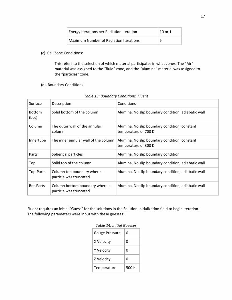
(c). Cell Zone Conditions:

This refers to the selection of which material participates in what zones. The “Air”

material was assigned to the “fluid” zone, and the “alumina” material was assigned to

the “particles” zone.

(d). Boundary Conditions

Table 13: Boundary Conditions, Fluent

Surface Description Conditions

Bottom

(bot)

Solid bottom of the column Alumina, No slip boundary condition, adiabatic wall

Column The outer wall of the annular

column

Alumina, No slip boundary condition, constant

temperature of 700 K

Innertube The inner annular wall of the column Alumina, No slip boundary condition, constant

temperature of 300 K

Parts Spherical particles Alumina, No slip boundary condition.

Top Solid top of the column Alumina, No slip boundary condition, adiabatic wall

Top‐Parts Column top boundary where a

particle was truncated

Alumina, No slip boundary condition, adiabatic wall

Bot‐Parts Column bottom boundary where a

particle was truncated

Alumina, No slip boundary condition, adiabatic wall

Fluent requires an initial "Guess" for the solutions in the Solution Initialization field to begin iteration.

The following parameters were input with these guesses:

Table 14: Initial Guesses

Gauge Pressure 0

X Velocity 0

Y Velocity 0

Z Velocity 0

Temperature 500 K

18

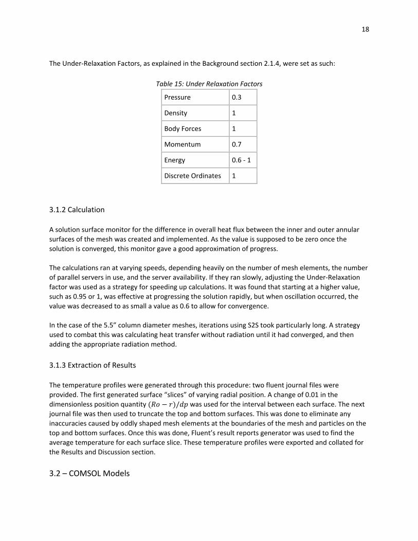
The Under‐Relaxation Factors, as explained in the Background section 2.1.4, were set as such:

Table 15: Under Relaxation Factors

Pressure 0.3

Density 1

Body Forces 1

Momentum 0.7

Energy 0.6 ‐ 1

Discrete Ordinates 1

3.1.2 Calculation

A solution surface monitor for the difference in overall heat flux between the inner and outer annular

surfaces of the mesh was created and implemented. As the value is supposed to be zero once the

solution is converged, this monitor gave a good approximation of progress.

The calculations ran at varying speeds, depending heavily on the number of mesh elements, the number

of parallel servers in use, and the server availability. If they ran slowly, adjusting the Under‐Relaxation

factor was used as a strategy for speeding up calculations. It was found that starting at a higher value,

such as 0.95 or 1, was effective at progressing the solution rapidly, but when oscillation occurred, the

value was decreased to as small a value as 0.6 to allow for convergence.

In the case of the 5.5” column diameter meshes, iterations using S2S took particularly long. A strategy

used to combat this was calculating heat transfer without radiation until it had converged, and then

adding the appropriate radiation method.

3.1.3 Extraction of Results

The temperature profiles were generated through this procedure: two fluent journal files were

provided. The first generated surface “slices” of varying radial position. A change of 0.01 in the

dimensionless position quantity / was used for the interval between each surface. The next

journal file was then used to truncate the top and bottom surfaces. This was done to eliminate any

inaccuracies caused by oddly shaped mesh elements at the boundaries of the mesh and particles on the

top and bottom surfaces. Once this was done, Fluent’s result reports generator was used to find the

average temperature for each surface slice. These temperature profiles were exported and collated for

the Results and Discussion section.

3.2 – COMSOL Models

19

COMSOL was set up with a 1‐dimensional axisymmetric steady‐state model to generate temperature

profiles based on the equations mentioned in the Background. The effective thermal conductivity

models, i.e. Equations 10 ‐ 21, were input as variables under the component section in COMSOL.

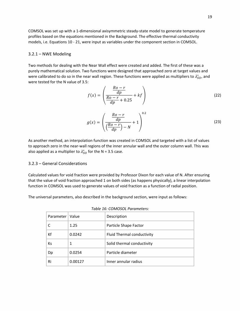
3.2.1 – NWE Modeling

Two methods for dealing with the Near Wall effect were created and added. The first of these was a

purely mathematical solution. Two functions were designed that approached zero at target values and

were calibrated to do so in the near wall region. These functions were applied as multipliers to ∗ , and

were tested for the N value of 3.5:

0.25

(22)

1

.

(23)

As another method, an interpolation function was created in COMSOL and targeted with a list of values

to approach zero in the near‐wall regions of the inner annular wall and the outer column wall. This was

also applied as a multiplier to ∗ for the N = 3.5 case.

3.2.3 – General Considerations

Calculated values for void fraction were provided by Professor Dixon for each value of N. After ensuring

that the value of void fraction approached 1 on both sides (as happens physically), a linear interpolation

function in COMSOL was used to generate values of void fraction as a function of radial position.

The universal parameters, also described in the background section, were input as follows:

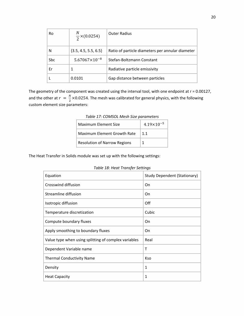
Table 16: COMOSOL Parameters:

Parameter Value Description

C 1.25 Particle Shape Factor

Kf 0.0242 Fluid Thermal conductivity

Ks 1 Solid thermal conductivity

Dp 0.0254 Particle diameter

Ri 0.00127 Inner annular radius

20

Ro

20.0254

Outer Radius

N {3.5, 4.5, 5.5, 6.5} Ratio of particle diameters per annular diameter

Sbc 5.67067 10 Stefan‐Boltzmann Constant

Er 1 Radiative particle emissivity

L 0.0101 Gap distance between particles

The geometry of the component was created using the interval tool, with one endpoint at r = 0.00127,

and the other at 0.0254. The mesh was calibrated for general physics, with the following

custom element size parameters:

Table 17: COMSOL Mesh Size parameters

Maximum Element Size 4.19 10

Maximum Element Growth Rate 1.1

Resolution of Narrow Regions 1

The Heat Transfer in Solids module was set up with the following settings:

Table 18: Heat Transfer Settings

Equation Study Dependent (Stationary)

Crosswind diffusion On

Streamline diffusion On

Isotropic diffusion Off

Temperature discretization Cubic

Compute boundary fluxes On

Apply smoothing to boundary fluxes On

Value type when using splitting of complex variables Real

Dependent Variable name T

Thermal Conductivity Name Kso

Density 1

Heat Capacity 1

21

Initial Value for Temperature 293.15 K

Inner Annular Temperature 300 K

Outer Annular Temperature 700 K

The solutions were displayed in graphical form with automatic y‐axis boundaries for temperature,

effective thermal conductivity, and void fraction, and the x‐axis was set to be a function of radial

position: – / . The comparisons created can be found in the Results and Discussion

section.

22

Chapter 4: Results and Discussion

4.1 – Discrete Ordinates versus Surface to Surface radiation

It was found that the Discrete Ordinates and Surface to Surface radiation methods produced practically

identical temperature profiles. This was the case for 3 out of the 4 values of N that were selected. For N

= 5.5, however, there was an irreconcilable simulation error (Seen in the appendices). Below is an

example of the similarity between S2S and DO, taken from N = 4.5:

Figure 2: Discrete Ordinates versus Surface to Surface methods, N=3.5

The Y‐axis in this graph shows the radial temperature, and the X‐axis shows a dimensionless form of

radial coordinate which ranges from 0 to N/2, where a lower value corresponds to a position closer to

the outer wall of the tube.

The close matching of the DO and S2S models indicates that they can be assumed to be generally

accurate and correct in predicting temperature behavior in these geometries.

300

350

400

450

500

550

600

650

700

0 0.5 1 1.5 2 2.5

T (K)

(Ro‐r)/dP

DO S2S

23

4.2 – Effect of Gaps

As mentioned in section 2.2.3, gaps were added to the ZBS model to be consistent between the CFD and

literature comparisons. It was found that the addition of gaps had a small, yet not quite negligible effect

on thermal conductivity. Thus, gaps were kept in the results for the remainder of the study. Figure 3

shows the difference in results that due to gaps in the ZBS model without radiation.

Figure 3: ZBS, Gaps versus no gaps, N=3.5

4.3 – Effect of Radiation

The ZBS method with the three radiation methods tested in this study (Damköhler, ZBS, and BB) are

compared in Figure 4. According to this result, only the Damköhler radiation method produces the

significant expected increase in temperature due to radiation, despite having some oscillations near the

walls that may represent problems with the equation or the need of mesh‐refinement. The other two

methods are only marginally different from the ZBS method without radiation, suggesting that they do

not accurately predict radiation behavior in stagnant packed beds.

300

350

400

450

500

550

600

650

700

0 0.2 0.4 0.6 0.8 1 1.2 1.4 1.6 1.8

T (K)

(Ro‐r)/dp

Derived Parallel nogap Derived Parallel gap

24

Figure 4: Comparison of ZBS varying Radiation Method, N=3.5

4.4 – ZBS versus CFD

Using the Damköhler radiation method, which shows the most promise for accuracy according to the

last result, CFD was compared to the ZBS model. There is a significant difference between the two; the

ZBS results are marginally lower than the CFD, as seen in Figure 5 for the N=3.5 case. However, when

corrected for the Near Wall Effect later on, the results matched with CFD very well over most of the

range, as seen in Figure 9.

300

350

400

450

500

550

600

650

700

0 0.2 0.4 0.6 0.8 1 1.2 1.4 1.6 1.8

T (K)

(Ro‐r)/dp

ZBS Radiation ZBS, No Radiation BB Radiation Damköhler Radiation

25

Figure 5: ZBS and Damköhler Radiation versus CFD, N=3.5

This and the result seen in Figure 9 indicates that the Damköhler radiation equation is a reasonably

accurate predictor of radiation behavior in packed beds, and further indicates that the ZBS base

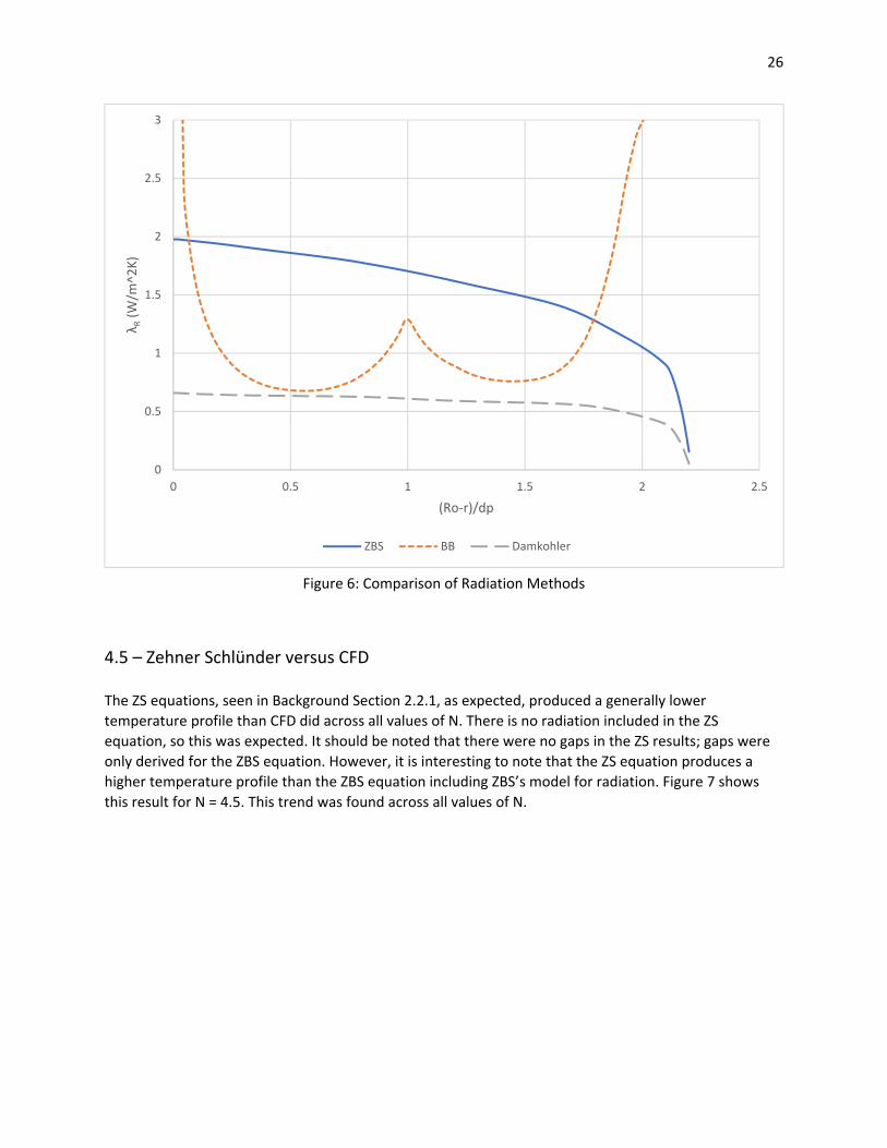
equation is also accurate. Figure 6 compares the variable λR as a function of radial position, and gives

some insight as to why Damköhler’s model is the most effective. While it is unknown what the

equivalent radiation thermal conductivity from CFD would have been, one can infer that the ZBS and BB

models are generally overestimates simply because of the mathematical parameters in the equation.

300

350

400

450

500

550

600

650

700

0 0.2 0.4 0.6 0.8 1 1.2 1.4 1.6 1.8

T (K)

(Ro‐r)/dp

DO S2S ZBS Damk

26

Figure 6: Comparison of Radiation Methods

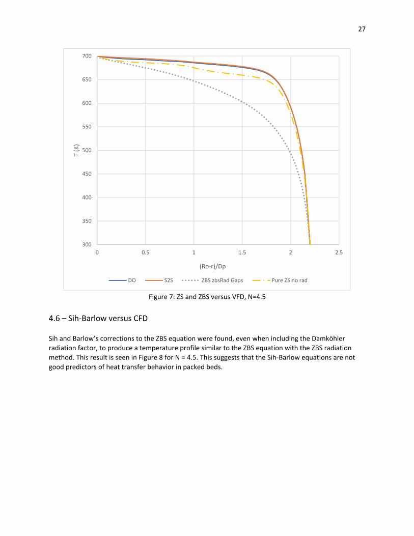
4.5 – Zehner Schlünder versus CFD

The ZS equations, seen in Background Section 2.2.1, as expected, produced a generally lower

temperature profile than CFD did across all values of N. There is no radiation included in the ZS

equation, so this was expected. It should be noted that there were no gaps in the ZS results; gaps were

only derived for the ZBS equation. However, it is interesting to note that the ZS equation produces a

higher temperature profile than the ZBS equation including ZBS’s model for radiation. Figure 7 shows

this result for N = 4.5. This trend was found across all values of N.

0

0.5

1

1.5

2

2.5

3

0 0.5 1 1.5 2 2.5

λ R(W

/m^2

K)

(Ro‐r)/dp

ZBS BB Damkohler

27

Figure 7: ZS and ZBS versus VFD, N=4.5

4.6 – Sih‐Barlow versus CFD

Sih and Barlow’s corrections to the ZBS equation were found, even when including the Damköhler

radiation factor, to produce a temperature profile similar to the ZBS equation with the ZBS radiation

method. This result is seen in Figure 8 for N = 4.5. This suggests that the Sih‐Barlow equations are not

good predictors of heat transfer behavior in packed beds.

300

350

400

450

500

550

600

650

700

0 0.5 1 1.5 2 2.5

T (K)

(Ro‐r)/Dp

DO S2S ZBS zbsRad Gaps Pure ZS no rad

28

Figure 8: Sih‐Barlow versus ZBS versus CFD, N=4.5

4.7 – Near Wall Effect

Out of the three methods tested for mitigating the Near Wall Effect, two produced results. The Tsotsas

equation was found to be incompatible with COMSOL due to its discontinuity, at least for the scope of

this project. The mathematical approach and interpolation function are compared below in Figure 9:

300

350

400

450

500

550

600

650

700

0 0.5 1 1.5 2 2.5

T (K)

(Ro‐r)/dP

DO S2S ZBS SB Damk ZBS zbsRad Gaps

29

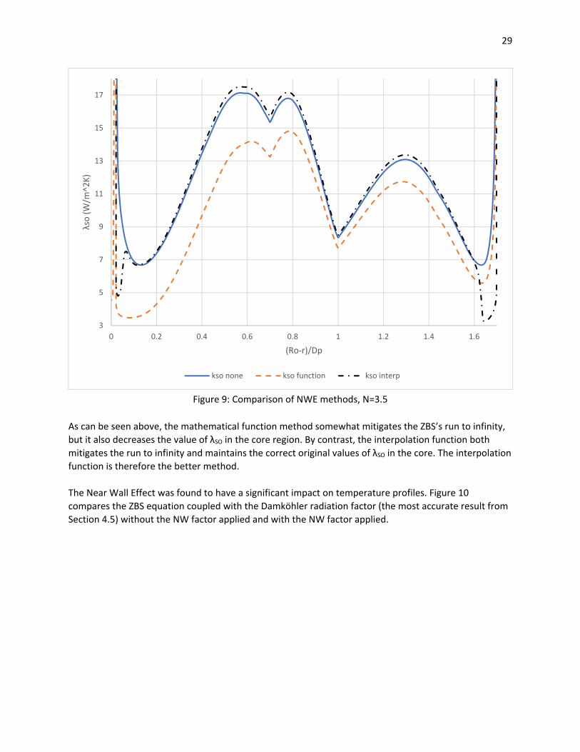
Figure 9: Comparison of NWE methods, N=3.5

As can be seen above, the mathematical function method somewhat mitigates the ZBS’s run to infinity,

but it also decreases the value of λSO in the core region. By contrast, the interpolation function both

mitigates the run to infinity and maintains the correct original values of λSO in the core. The interpolation

function is therefore the better method.

The Near Wall Effect was found to have a significant impact on temperature profiles. Figure 10

compares the ZBS equation coupled with the Damköhler radiation factor (the most accurate result from

Section 4.5) without the NW factor applied and with the NW factor applied.

3

5

7

9

11

13

15

17

0 0.2 0.4 0.6 0.8 1 1.2 1.4 1.6

λso (W/m

^2K)

(Ro‐r)/Dp

kso none kso function kso interp

30

Figure 10: ZBS/Damköhler/NWE versus CFD, N=3.5

It was found that the addition of the Near Wall Effect factor produced results that matched almost

identically with CFD for a great portion of the range tested. However, towards the inner tube wall, the

ZBS/Damk/NWE combination overpredicted the temperature relative to CFD. Figure 10 shows the result

for N=3.5.

The near wall effect has significant impact on the endpoint ranges for the temperature profiles; the

reduction in thermal conductivity corresponds to an increase in temperature. As mentioned earlier, the

near wall region is defined as the distance within 1 particle radius from any wall. For low values of N

(such as the values in this study), this region encompasses a significant portion of the entire distance.

Furthermore, small variations in the endpoint values can have compounding effects for the whole

domain, similar to how changing the slope of a line increasingly changes deviation from its original

location as distance from the origin increases.

300

350

400

450

500

550

600

650

700

0 0.2 0.4 0.6 0.8 1 1.2 1.4 1.6 1.8

T (K)

(Ro‐r)/dp

DO S2S ZBS Damk ZBS damk NWint

31

Chapter 5 – Conclusions and Recommendations

Based on the models tested in this study, it is reasonable to conclude that the Discrete Ordinates,

Surface to Surface, and ZBS/Damköhler/CasoNWF models accurately predict temperature behavior in

small stagnant packed beds. The ZBS radiation model, Breitbach‐Barthels, Zehner‐Schlünder, and Sih‐

Barlow models do not accurately predict temperature behavior in small stagnant packed beds.

However, there were significant simplifications made in this study. The further exploration in these

areas are possible expansions for further research. Possible topics for expansion include: variation of

particle shape from spheres, variation of bed size, the use of binary or ternary particle mixtures, the

presence of a different form of heat generation (i.e. a volumetric or catalytic reaction), and the removal

of the innertube or other alteration of geometry.

Other areas of recommended work include the expansion of CFD model size assuming the availability of

processing power. There are not likely any actual packed beds with an average of three to four particles

fitting in the column diameter, and the behavior of larger CFD models is yet unknown due to the

availability of computing power. As technology stands today, it is not practical to test large or actual‐

sized models, but it may be possible to do so in the future.

Despite the ZBS equations being widely cited, there are many other models for calculating effective

thermal conductivity. Work beyond ZBS was beyond the scope of this project, but more accurate results

may be awaiting whomever tries the correct combination of baseline equation, radiation conductivity

model, and method for mitigating the near wall effect. On the CFD side, there are several alternate

radiation methods that could be tested. This study may be hitting the tip of the iceberg of accurate

predictions of heat transfer in stagnant packed beds.

32

Chapter 6 – References

ANSYS® Academic Research, Release 16.2, Help System, Modeling Heat Transfer Guide, ANSYS, Inc.

Bauer, R., Schlünder, E. U., 1978. Part I: Effective radial thermal conductivity o fpackings in gas flow, Part

II: Thermal conductivity of the packing fraction without gas flow. International Chemical Engineering 18,

189–204.

Breitbach, G., Barthels, H., 1980. The radiant heat transfer in the high temperature reactor core after

failure of the afterheat removal systems. Nuclear Technology 49, 392–399.

DiNino, A., Hartzell, E., Judge, K., Morgan, A., 2013. Heating and Cooling in a Packed Bed, Worcester

Polytechnic Institute.

G. Damkohler, in Eucken and Jakob (eds.), 1937. Der Chemie‐Ingenieur, Vol. 3, Part 1, Akad. Verlag,

Leipzig.

Gurnon, A., Lirette, A., Schaaf, C., Vitello N., 2009. Effective Radial Thermal Conductivity in Fixed‐Bed

Reactor Tubes, Worcester Polytechnic Institute.

Hengst, G., 1934. Die Wärmeleitfähigkeit pulverförmiger Stoffe bei hohem Gasdruck, Ph.D. Thesis,

University of Munich.

Sih, S. S., and Barlow, J. W., 2004. "The prediction of the emissivity and thermal conductivity of powder

beds," Particulate Science and Technology, 22, pp. 291‐304.

Thurgood, C.P., Amphlett, J. C., Mann, R. F., Peppley, B. A., 2004. Radiative heat transfer in packed‐beds:

The near‐wall region. In: AIChE Spring National Meeting, New Orleans April 25–29, Paper No. T2007‐16e.

Tsotsas, E., In: Hewitt, G.F. (Ed.), 2002. Heat Exchanger Design Handbook. Begell House Publishing,

Section 2.8.2.

Zehner, P., Schlünder, E.U., 1970. Wärmeleitfähigkeit von Schüttungen bei mäƥigen Temperaturen,

Chemie Ingenieur Technik 42, 933–941.

33

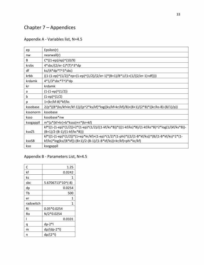
Chapter 7 – Appendices

Appendix A ‐ Variables list, N=4.5

ep Epsilon(r)

nw nearwall(r)

B C*((1‐ep)/ep)^(10/9)

krzbs 4*sbc/(2/er‐1)*(T)^3*dp

df ks/(4*dp*T^3*sbc)

krbb ((1‐(1‐ep)^(1/2))*ep+(1‐ep)^(1/2)/(2/er‐1)*(B+1)/B*1/(1+(1/((2/er‐1)+df))))

krdamk 4*1/3*sbc*T^3*dp

kr krdamk

a (1‐(1‐ep)^(1/2))

b (1‐ep)^(1/2)

p 1+(kr/kf‐B)*kf/ks

kssobase 2/p*((B*(ks/kf+kr/kf‐1))/(p^2*ks/kf)*log((ks/kf+kr/kf)/B)+(B+1)/(2*B)*((kr/ks‐B)‐(B/1)/p))

kssonorm kssobase

ksso kssobase*nw

ksogappll m*(a*(kf+kr)+b*ksso)+n*(kr+kf)

ksoZS kf*((1‐(1‐ep)^(1/2))+2*(1‐ep)^(1/2)/((1‐kf/ks*B))*(((1‐kf/ks)*B)/(1‐kf/ks*B)^2*log(1/(kf/ks*B))‐(B+1)/2‐(B‐1)/(1‐kf/ks*B)))

ksoSB kf*((1‐(1‐ep)^(1/2))*(1+ep*kr/kf)+(1‐ep)^(1/2)*(1‐phi)*((2/(1‐B*kf/ks))*(B/(1‐B*kf/ks)^2*(1‐kf/ks)*log(ks/(B*kf))‐(B+1)/2‐(B‐1)/(1‐B*kf/ks))+kr/kf)+phi*kc/kf)

kso ksogappll

Appendix B ‐ Parameters List, N=4.5

C 1.25

kf 0.0242

ks 1

sbc 5.6706713*10^(‐8)

dp 0.0254

Tb 500

er 1

radswitch 1

Ri 0.05*0.0254

Ro N/2*0.0254

l 0.0101

q dp‐2*l

m dp/(dp‐2*l)

n dp/(2*l)

34

N 4.5

Appendix C – Void Fraction Data N = 3.5 0.00127 0.99999999999 0.00254 0.79309213125 0.002794 0.76226660625 0.003048 0.7341451375 0.003302 0.70849335 0.003556 0.685034125 0.00381 0.66349688125 0.004064 0.64377650625 0.004318 0.6244233875 0.004572 0.604202 0.004826 0.58549058125 0.00508 0.5682303 0.005334 0.5523406875 0.005588 0.537589075 0.005842 0.52399760625 0.006096 0.5114662625 0.00635 0.4999069 0.006604 0.48934728125 0.006858 0.47964555 0.007112 0.470804275 0.007366 0.4628064625 0.00762 0.4556215375 0.007874 0.44913810625 0.008128 0.44221878125 0.008382 0.434702875 0.008636 0.4279484375 0.00889 0.421808375 0.009144 0.4163053125 0.009398 0.411496375 0.009652 0.407342625 0.009906 0.403785 0.01016 0.4007781875 0.010414 0.398320375 0.010668 0.396413 0.010922 0.3950179375 0.011176 0.394026625 0.01143 0.3935399375 0.011684 0.393585875 0.011938 0.394085625 0.012192 0.39505975 0.012446 0.396368375 0.0127 0.398159375 0.012954 0.400369125 0.013208 0.4029654375 0.013462 0.405947625 0.013716 0.409367125 0.01397 0.4131783125 0.014224 0.417361625 0.014478 0.4219135 0.014732 0.4268580625 0.014986 0.432156375 0.01524 0.43777424375 0.015494 0.44373750625 0.015748 0.450013875 0.016002 0.45661216875

0.016256 0.46354085 0.01651 0.4707831125 0.016764 0.47827720625 0.017018 0.4860779625 0.017272 0.4941867 0.017526 0.50255870625 0.01778 0.51116258125 0.018034 0.52005893125 0.018288 0.5292459125 0.018542 0.53867894375 0.018796 0.54833680625 0.01905 0.55828869375 0.019304 0.541926025 0.019558 0.52090960625 0.019812 0.50055635 0.020066 0.481400075 0.02032 0.46355211875 0.020574 0.44686538125 0.020828 0.431482125 0.021082 0.4173823125 0.021336 0.404387 0.02159 0.3924584375 0.021844 0.381466125 0.022098 0.37130175 0.022352 0.3620270625 0.022606 0.3536336875 0.02286 0.3460925625 0.023114 0.3394385625 0.023368 0.333719125 0.023622 0.3289189375 0.023876 0.325157125 0.02413 0.32246475 0.024384 0.3208545625 0.024638 0.3202685 0.024892 0.32066425 0.025146 0.3219095 0.0254 0.3239681875 0.025654 0.3268769375 0.025908 0.3307015625 0.026162 0.33544425 0.026416 0.3410864375 0.02667 0.3460789375 0.026924 0.3410376875 0.027178 0.3367096875 0.027432 0.3323676875 0.027686 0.327925375 0.02794 0.3241820625 0.028194 0.321175375 0.028448 0.318811125 0.028702 0.3170518125 0.028956 0.3159325625 0.02921 0.315398125 0.029464 0.3153948125 0.029718 0.3152575 0.029972 0.314944 0.030226 0.3151591875

0.03048 0.3158651875 0.030734 0.31706125 0.030988 0.3187788125 0.031242 0.3210373125 0.031496 0.3238091875 0.03175 0.32709575 0.032004 0.3309264375 0.032258 0.33533125 0.032512 0.3402668125 0.032766 0.3457174375 0.03302 0.351689 0.033274 0.358192125 0.033528 0.3644265625 0.033782 0.37074775 0.034036 0.377548125 0.03429 0.3848115 0.034544 0.3925763125 0.034798 0.4008024375 0.035052 0.409458625 0.035306 0.418549375 0.03556 0.4281049375 0.035814 0.43811488125 0.036068 0.44855105625 0.036322 0.4593749625 0.036576 0.47061485 0.03683 0.48230648125 0.037084 0.49439519375 0.037338 0.5068683 0.037592 0.51973211875 0.037846 0.53303450625 0.0381 0.54675913125 0.038354 0.56084161875 0.038608 0.57529270625 0.038862 0.5901455875 0.039116 0.605341075 0.03937 0.62086245625 0.039624 0.63680210625 0.039878 0.6531893625 0.040132 0.6698586625 0.040386 0.68687745625 0.04064 0.704375625 0.040894 0.7221398625 0.041148 0.7401959625 0.041402 0.7588906 0.041656 0.77768883125 0.04191 0.79692500625 0.042164 0.81661556875 0.042418 0.83635310625 0.042672 0.85666495625 0.042926 0.8769414875 0.04318 0.89778285 0.043434 0.918690175 0.043688 0.944253725 0.043942 0.999999999 0.044196 0.999999999

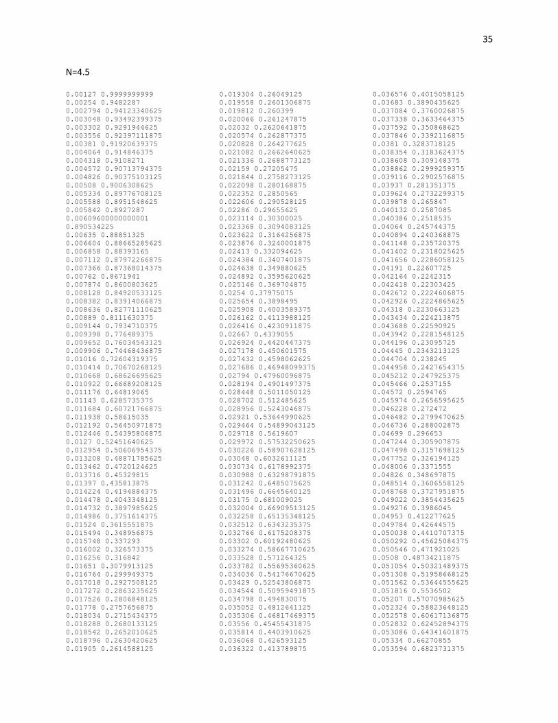
35

N=4.5 0.00127 0.9999999999 0.00254 0.9482287 0.002794 0.94123340625 0.003048 0.93492399375 0.003302 0.9291944625 0.003556 0.92397111875 0.00381 0.91920639375 0.004064 0.914846375 0.004318 0.9108271 0.004572 0.90713794375 0.004826 0.90375103125 0.00508 0.9006308625 0.005334 0.89776708125 0.005588 0.8951548625 0.005842 0.8927287 0.00609600000000001 0.890534225 0.00635 0.88851325 0.006604 0.88665285625 0.006858 0.88393165 0.007112 0.87972266875 0.007366 0.87368014375 0.00762 0.8671941 0.007874 0.8600803625 0.008128 0.84920533125 0.008382 0.83914066875 0.008636 0.82771110625 0.00889 0.8111630375 0.009144 0.7934710375 0.009398 0.776489375 0.009652 0.76034543125 0.009906 0.74468436875 0.01016 0.72604319375 0.010414 0.70670268125 0.010668 0.68626695625 0.010922 0.66689208125 0.011176 0.64819065 0.01143 0.6285735375 0.011684 0.60721766875 0.011938 0.58615035 0.012192 0.56450971875 0.012446 0.54395806875 0.0127 0.52451640625 0.012954 0.50606954375 0.013208 0.48871785625 0.013462 0.4720124625 0.013716 0.45329815 0.01397 0.435813875 0.014224 0.4194884375 0.014478 0.4043348125 0.014732 0.3897985625 0.014986 0.3751614375 0.01524 0.3615551875 0.015494 0.348956875 0.015748 0.337293 0.016002 0.326573375 0.016256 0.316842 0.01651 0.3079913125 0.016764 0.299949375 0.017018 0.2927508125 0.017272 0.2863235625 0.017526 0.2806848125 0.01778 0.2757656875 0.018034 0.2715434375 0.018288 0.2680133125 0.018542 0.2652010625 0.018796 0.2630420625 0.01905 0.2614588125

0.019304 0.26049125 0.019558 0.2601306875 0.019812 0.260399 0.020066 0.261247875 0.02032 0.2620641875 0.020574 0.262877375 0.020828 0.264277625 0.021082 0.2662640625 0.021336 0.2688773125 0.02159 0.27205475 0.021844 0.2758273125 0.022098 0.280168875 0.022352 0.2850565 0.022606 0.290528125 0.02286 0.29655625 0.023114 0.30300025 0.023368 0.3094083125 0.023622 0.3164256875 0.023876 0.3240001875 0.02413 0.332094625 0.024384 0.3407401875 0.024638 0.349880625 0.024892 0.3595620625 0.025146 0.369704875 0.0254 0.37975075 0.025654 0.3898495 0.025908 0.4003589375 0.026162 0.4113988125 0.026416 0.4230911875 0.02667 0.4339055 0.026924 0.4420447375 0.027178 0.450601575 0.027432 0.4598062625 0.027686 0.46948099375 0.02794 0.47960096875 0.028194 0.4901497375 0.028448 0.5011050125 0.028702 0.512485625 0.028956 0.5243046875 0.02921 0.53644990625 0.029464 0.54899043125 0.029718 0.5619607 0.029972 0.57532250625 0.030226 0.58907628125 0.03048 0.6032611125 0.030734 0.6178992375 0.030988 0.63298791875 0.031242 0.6485075625 0.031496 0.6645640125 0.03175 0.681009025 0.032004 0.66909513125 0.032258 0.65135348125 0.032512 0.6343235375 0.032766 0.6175208375 0.03302 0.60192480625 0.033274 0.58667710625 0.033528 0.571264325 0.033782 0.55695360625 0.034036 0.54176670625 0.03429 0.52543806875 0.034544 0.50959491875 0.034798 0.494830075 0.035052 0.4812641125 0.035306 0.46817469375 0.03556 0.45455431875 0.035814 0.4403910625 0.036068 0.426593125 0.036322 0.413789875

0.036576 0.4015058125 0.03683 0.3890435625 0.037084 0.3760026875 0.037338 0.3633464375 0.037592 0.350868625 0.037846 0.3392116875 0.0381 0.3283718125 0.038354 0.3183624375 0.038608 0.309148375 0.038862 0.2999259375 0.039116 0.2902576875 0.03937 0.281351375 0.039624 0.2732299375 0.039878 0.265847 0.040132 0.2587085 0.040386 0.2518535 0.04064 0.245744375 0.040894 0.240368875 0.041148 0.235720375 0.041402 0.2318025625 0.041656 0.2286058125 0.04191 0.22607725 0.042164 0.2242315 0.042418 0.22303425 0.042672 0.2224606875 0.042926 0.2224865625 0.04318 0.2230663125 0.043434 0.224213875 0.043688 0.22590925 0.043942 0.2281548125 0.044196 0.23095725 0.04445 0.2343213125 0.044704 0.238245 0.044958 0.2427654375 0.045212 0.247925375 0.045466 0.2537155 0.04572 0.2594765 0.045974 0.2656595625 0.046228 0.272472 0.046482 0.2799470625 0.046736 0.288002875 0.04699 0.296653 0.047244 0.305907875 0.047498 0.3157698125 0.047752 0.326194125 0.048006 0.3371555 0.04826 0.348697875 0.048514 0.3606558125 0.048768 0.3727951875 0.049022 0.3854435625 0.049276 0.3986045 0.04953 0.412277625 0.049784 0.42644575 0.050038 0.4410707375 0.050292 0.45625084375 0.050546 0.471921025 0.0508 0.48734211875 0.051054 0.50321489375 0.051308 0.51958668125 0.051562 0.53644555625 0.051816 0.5536502 0.05207 0.57070985625 0.052324 0.58823648125 0.052578 0.60617136875 0.052832 0.62452894375 0.053086 0.64341601875 0.05334 0.66270855 0.053594 0.6823731375

36

0.053848 0.70259895625 0.054102 0.72318696875 0.054356 0.74416965 0.05461 0.7656663625 0.054864 0.78746339375

0.055118 0.80968493125 0.055372 0.83229528125 0.055626 0.8552294375 0.05588 0.87865806875 0.056134 0.90256161875

0.056388 0.93061071875 0.056642 0.99999999999 0.056896 0.99999999999

N = 5.5 0.00127 0.99999999 0.00254 0.81985121875 0.002794 0.78800893125 0.003048 0.75925516875 0.003302 0.73317629375 0.003556 0.7094571875 0.00381 0.68765184375 0.004064 0.6673957125 0.004318 0.6487221125 0.004572 0.62840220625 0.004826 0.60568234375 0.00508 0.58481770625 0.005334 0.56588134375 0.005588 0.54841655625 0.005842 0.53245288125 0.00609600000000001 0.51523625625 0.00635 0.49901014375 0.00660399999999999 0.4838613875 0.006858 0.46978694375 0.007112 0.45692926875 0.007366 0.4450243125 0.00761999999999999 0.434044 0.007874 0.4240405 0.008128 0.413899625 0.008382 0.40140025 0.008636 0.386924875 0.00889 0.3714816875 0.009144 0.357160625 0.009398 0.34380025 0.009652 0.3315793125 0.009906 0.3203356875 0.01016 0.3100596875 0.010414 0.300645125 0.010668 0.2920855 0.010922 0.2843275625 0.011176 0.2773726875 0.01143 0.2712479375 0.011684 0.2659145625 0.011938 0.2612865 0.012192 0.2573975625 0.012446 0.25347625 0.0127 0.2491556875 0.012954 0.245644625 0.013208 0.2428474375 0.013462 0.240801375 0.013716 0.2395015 0.01397 0.239009625 0.014224 0.23921275 0.014478 0.240120375 0.014732 0.241675125 0.014986 0.243820375 0.01524 0.246573 0.015494 0.2498654375 0.015748 0.2536994375 0.016002 0.258082 0.016256 0.26300925 0.01651 0.26846375 0.016764 0.2744254375 0.017018 0.2809034375

0.017272 0.287911 0.017526 0.2954265 0.01778 0.3034305625 0.018034 0.3118806875 0.018288 0.3207864375 0.018542 0.330184625 0.018796 0.339993625 0.01905 0.3501970625 0.019304 0.360855375 0.019558 0.371966375 0.019812 0.3834639375 0.020066 0.3952985 0.02032 0.406996375 0.020574 0.41846825 0.020828 0.42897275 0.021082 0.438596425 0.021336 0.4468713375 0.02159 0.4545919875 0.021844 0.46127831875 0.022098 0.4677628875 0.022352 0.47395556875 0.022606 0.48002678125 0.02286 0.48183149375 0.023114 0.48096573125 0.023368 0.48047071875 0.023622 0.4809463625 0.023876 0.48209899375 0.02413 0.48255729375 0.024384 0.48029744375 0.024638 0.476678075 0.024892 0.473536375 0.025146 0.47129893125 0.0254 0.4683688875 0.025654 0.46649289375 0.025908 0.4655879125 0.026162 0.46560013125 0.026416 0.4663398875 0.02667 0.4670634875 0.026924 0.45930361875 0.027178 0.45123630625 0.027432 0.44212508125 0.027686 0.43313175 0.02794 0.422402625 0.028194 0.4121866875 0.028448 0.4028950625 0.028702 0.3946038125 0.028956 0.3873308125 0.02921 0.3809640625 0.029464 0.37558425 0.029718 0.3704074375 0.029972 0.363864625 0.030226 0.357066125 0.03048 0.351096625 0.030734 0.3459535625 0.030988 0.341545875 0.031242 0.3375296875 0.031496 0.3325015 0.03175 0.32823725 0.032004 0.3246535 0.032258 0.3217443125 0.032512 0.31953725 0.032766 0.318077625

0.03302 0.317374875 0.033274 0.3174110625 0.033528 0.3168921875 0.033782 0.3149076875 0.034036 0.311736375 0.03429 0.308600875 0.034544 0.3061095 0.034798 0.3042643125 0.035052 0.303008625 0.035306 0.3023500625 0.03556 0.302274875 0.035814 0.3028318125 0.036068 0.30399325 0.036322 0.30576375 0.036576 0.3082005625 0.03683 0.311202875 0.037084 0.3147615 0.037338 0.3188768125 0.037592 0.323562375 0.037846 0.32805575 0.0381 0.33279875 0.038354 0.33805875 0.038608 0.343840125 0.038862 0.350143875 0.039116 0.356955875 0.03937 0.36429575 0.039624 0.372154 0.039878 0.3805211875 0.040132 0.3893949375 0.040386 0.398760125 0.04064 0.4086298125 0.040894 0.4189731875 0.041148 0.4298109375 0.041402 0.44113058125 0.041656 0.45292598125 0.04191 0.4651656125 0.042164 0.47787391875 0.042418 0.49105620625 0.042672 0.50469303125 0.042926 0.5188359 0.04318 0.5334447 0.043434 0.5485275375 0.043688 0.564073625 0.043942 0.5801200875 0.044196 0.59668943125 0.04445 0.61386945625 0.044704 0.604282825 0.044958 0.5908742875 0.045212 0.57859358125 0.045466 0.5673930625 0.04572 0.55689221875 0.045974 0.547231375 0.046228 0.5372948625 0.046482 0.52714836875 0.046736 0.5165778375 0.04699 0.50636744375 0.047244 0.495754125 0.047498 0.48603338125 0.047752 0.47672241875 0.048006 0.4673011875 0.04826 0.4550513 0.048514 0.44223255

37

0.048768 0.430267625 0.049022 0.419401875 0.049276 0.4096775 0.04953 0.399280875 0.049784 0.387216875 0.050038 0.374921 0.050292 0.36282075 0.050546 0.3511603125 0.0508 0.3392864375 0.051054 0.32818025 0.051308 0.3177978125 0.051562 0.3081621875 0.051816 0.298911125 0.05207 0.2900644375 0.052324 0.2819861875 0.052578 0.2741383125 0.052832 0.2668863125 0.053086 0.2596801875 0.05334 0.2526370625 0.053594 0.2464113125 0.053848 0.2410046875 0.054102 0.2363961875 0.054356 0.2325415 0.05461 0.22945025 0.054864 0.2270895625 0.055118 0.22483675 0.055372 0.2231914375 0.055626 0.2221489375

0.05588 0.2217039375 0.056134 0.221839125 0.056388 0.22252225 0.056642 0.2233540625 0.056896 0.2244525 0.05715 0.2261055625 0.057404 0.2283271875 0.057658 0.2311369375 0.057912 0.234525875 0.058166 0.2385345 0.05842 0.2431986875 0.058674 0.2485510625 0.058928 0.254026625 0.059182 0.260105 0.059436 0.266874 0.05969 0.2743198125 0.059944 0.2824250625 0.060198 0.2911320625 0.060452 0.3004184375 0.060706 0.310312 0.06096 0.32081725 0.061214 0.3318900625 0.061468 0.34348775 0.061722 0.355653375 0.061976 0.3684153125 0.06223 0.38173125 0.062484 0.3955773125 0.062738 0.4099494375

0.062992 0.424906 0.063246 0.44041204375 0.0635 0.456406 0.063754 0.4728944875 0.064008 0.4899446375 0.064262 0.50752311875 0.064516 0.52555668125 0.06477 0.54409545625 0.065024 0.5631946 0.065278 0.58273649375 0.065532 0.60268851875 0.065786 0.62315699375 0.06604 0.64412000625 0.066294 0.66549119375 0.066548 0.68734836875 0.066802 0.7097223125 0.067056 0.732385425 0.06731 0.7555764625 0.067564 0.77915704375 0.067818 0.80291756875 0.068072 0.8271126 0.068326 0.85141498125 0.06858 0.87616998125 0.068834 0.90097874375 0.069088 0.9291597875 0.069342 0.999999 0.069596 0.99999 0.06985 0.9999999

N = 6.5 0.00127 0.99999999 0.00254 0.7915784125 0.002794 0.7623690375 0.003048 0.73592021875 0.003302 0.7118696 0.003556 0.689906775 0.00381 0.66987466875 0.004064 0.65173188125 0.004318 0.6351535 0.004572 0.6199713625 0.004826 0.60603886875 0.00508 0.59324526875 0.005334 0.581492575 0.005588 0.57070878125 0.005842 0.5608605125 0.00609600000000001 0.55186945 0.00635 0.54365575625 0.00660399999999999 0.5361692875 0.006858 0.5270274875 0.007112 0.51565599375 0.007366 0.50510376875 0.00761999999999999 0.49551391875 0.007874 0.48669779375 0.008128 0.47856575 0.008382 0.471136275 0.008636 0.46443963125 0.00889 0.45837646875 0.009144 0.4528867 0.009398 0.44803715 0.009652 0.443746925 0.009906 0.4399623875 0.01016 0.4367798125 0.010414 0.4341770625 0.010668 0.4320619375 0.010922 0.4304735 0.011176 0.429426625

0.01143 0.427763375 0.011684 0.425916375 0.011938 0.4245858125 0.012192 0.4236819375 0.012446 0.42158925 0.0127 0.41996875 0.012954 0.4182764375 0.013208 0.4139661875 0.013462 0.4083401875 0.013716 0.4010745625 0.01397 0.394842375 0.014224 0.3893715625 0.014478 0.3831576875 0.014732 0.377608375 0.014986 0.3728300625 0.01524 0.3688098125 0.015494 0.3645923125 0.015748 0.36040375 0.016002 0.354308125 0.016256 0.3477176875 0.01651 0.340804 0.016764 0.3340871875 0.017018 0.32819075 0.017272 0.323227375 0.017526 0.3189584375 0.01778 0.315510125 0.018034 0.3126089375 0.018288 0.3093990625 0.018542 0.3069206875 0.018796 0.3052225 0.01905 0.303995875 0.019304 0.302115 0.019558 0.301008125 0.019812 0.3006051875 0.020066 0.300920625 0.02032 0.301885875 0.020574 0.3035049375 0.020828 0.305711375 0.021082 0.308569875

0.021336 0.3116896875 0.02159 0.3146821875 0.021844 0.31705975 0.022098 0.3193238125 0.022352 0.322518625 0.022606 0.3265403125 0.02286 0.3312506875 0.023114 0.3357508125 0.023368 0.3410418125 0.023622 0.34706575 0.023876 0.353884875 0.02413 0.361358625 0.024384 0.3691914375 0.024638 0.376836375 0.024892 0.384116 0.025146 0.39136525 0.0254 0.3985596875 0.025654 0.406182875 0.025908 0.4143350625 0.026162 0.4230795625 0.026416 0.4322588125 0.02667 0.43928861875 0.026924 0.4350405625 0.027178 0.4299556875 0.027432 0.4262454375 0.027686 0.4233394375 0.02794 0.4210186875 0.028194 0.41932425 0.028448 0.41822 0.028702 0.417709625 0.028956 0.4178138125 0.02921 0.417754 0.029464 0.418081375 0.029718 0.4189736875 0.029972 0.4204610625 0.030226 0.422555875 0.03048 0.425183875 0.030734 0.42839775 0.030988 0.432169375

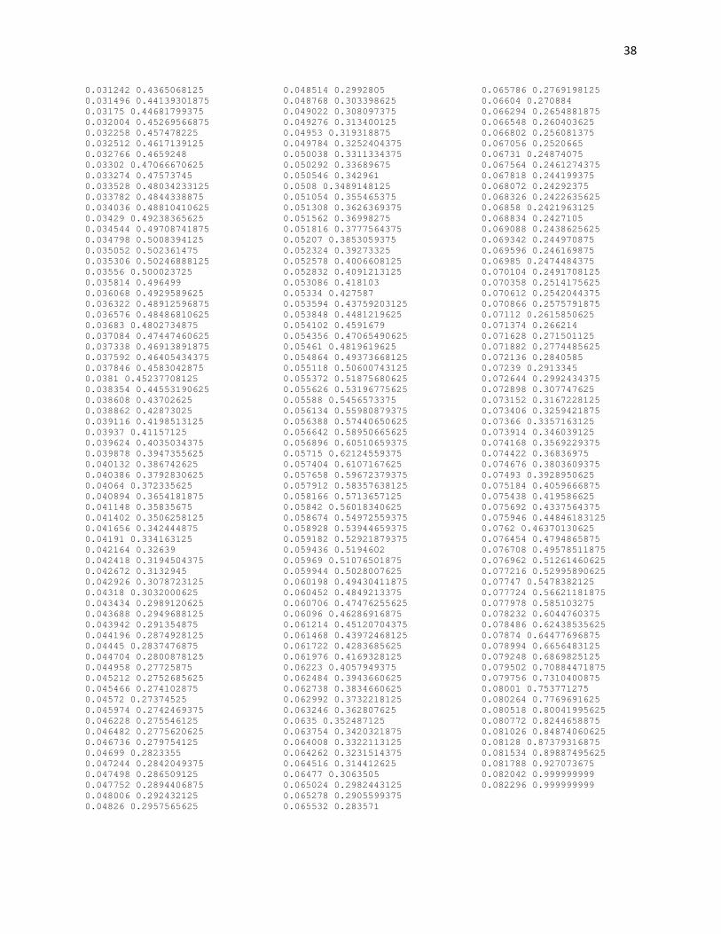
38

0.031242 0.4365068125 0.031496 0.44139301875 0.03175 0.44681799375 0.032004 0.45269566875 0.032258 0.457478225 0.032512 0.4617139125 0.032766 0.4659248 0.03302 0.47066670625 0.033274 0.47573745 0.033528 0.48034233125 0.033782 0.4844338875 0.034036 0.48810410625 0.03429 0.49238365625 0.034544 0.49708741875 0.034798 0.5008394125 0.035052 0.502361475 0.035306 0.50246888125 0.03556 0.500023725 0.035814 0.496499 0.036068 0.4929589625 0.036322 0.48912596875 0.036576 0.48486810625 0.03683 0.4802734875 0.037084 0.47447460625 0.037338 0.46913891875 0.037592 0.46405434375 0.037846 0.4583042875 0.0381 0.45237708125 0.038354 0.44553190625 0.038608 0.43702625 0.038862 0.42873025 0.039116 0.4198513125 0.03937 0.41157125 0.039624 0.4035034375 0.039878 0.3947355625 0.040132 0.386742625 0.040386 0.3792830625 0.04064 0.372335625 0.040894 0.3654181875 0.041148 0.35835675 0.041402 0.3506258125 0.041656 0.342444875 0.04191 0.334163125 0.042164 0.32639 0.042418 0.3194504375 0.042672 0.3132945 0.042926 0.3078723125 0.04318 0.3032000625 0.043434 0.2989120625 0.043688 0.2949688125 0.043942 0.291354875 0.044196 0.2874928125 0.04445 0.2837476875 0.044704 0.2800878125 0.044958 0.27725875 0.045212 0.2752685625 0.045466 0.274102875 0.04572 0.27374525 0.045974 0.2742469375 0.046228 0.275546125 0.046482 0.2775620625 0.046736 0.279754125 0.04699 0.2823355 0.047244 0.2842049375 0.047498 0.286509125 0.047752 0.2894406875 0.048006 0.292432125 0.04826 0.2957565625

0.048514 0.2992805 0.048768 0.303398625 0.049022 0.308097375 0.049276 0.313400125 0.04953 0.319318875 0.049784 0.3252404375 0.050038 0.3311334375 0.050292 0.33689675 0.050546 0.342961 0.0508 0.3489148125 0.051054 0.355465375 0.051308 0.3626369375 0.051562 0.36998275 0.051816 0.3777564375 0.05207 0.3853059375 0.052324 0.39273325 0.052578 0.4006608125 0.052832 0.4091213125 0.053086 0.418103 0.05334 0.427587 0.053594 0.43759203125 0.053848 0.4481219625 0.054102 0.4591679 0.054356 0.47065490625 0.05461 0.4819619625 0.054864 0.49373668125 0.055118 0.50600743125 0.055372 0.51875680625 0.055626 0.53196775625 0.05588 0.5456573375 0.056134 0.55980879375 0.056388 0.57440650625 0.056642 0.58950665625 0.056896 0.60510659375 0.05715 0.62124559375 0.057404 0.6107167625 0.057658 0.59672379375 0.057912 0.58357638125 0.058166 0.5713657125 0.05842 0.56018340625 0.058674 0.54972559375 0.058928 0.53944659375 0.059182 0.52921879375 0.059436 0.5194602 0.05969 0.51076501875 0.059944 0.5028007625 0.060198 0.49430411875 0.060452 0.4849213375 0.060706 0.47476255625 0.06096 0.46286916875 0.061214 0.45120704375 0.061468 0.43972468125 0.061722 0.4283685625 0.061976 0.4169328125 0.06223 0.4057949375 0.062484 0.3943660625 0.062738 0.3834660625 0.062992 0.3732218125 0.063246 0.362807625 0.0635 0.352487125 0.063754 0.3420321875 0.064008 0.3322113125 0.064262 0.3231514375 0.064516 0.314412625 0.06477 0.3063505 0.065024 0.2982443125 0.065278 0.2905599375 0.065532 0.283571

0.065786 0.2769198125 0.06604 0.270884 0.066294 0.2654881875 0.066548 0.260403625 0.066802 0.256081375 0.067056 0.2520665 0.06731 0.24874075 0.067564 0.2461274375 0.067818 0.244199375 0.068072 0.24292375 0.068326 0.2422635625 0.06858 0.2421963125 0.068834 0.2427105 0.069088 0.2438625625 0.069342 0.244970875 0.069596 0.246169875 0.06985 0.2474484375 0.070104 0.2491708125 0.070358 0.2514175625 0.070612 0.2542044375 0.070866 0.2575791875 0.07112 0.2615850625 0.071374 0.266214 0.071628 0.271501125 0.071882 0.2774485625 0.072136 0.2840585 0.07239 0.2913345 0.072644 0.2992434375 0.072898 0.307747625 0.073152 0.3167228125 0.073406 0.3259421875 0.07366 0.3357163125 0.073914 0.346039125 0.074168 0.3569229375 0.074422 0.36836975 0.074676 0.3803609375 0.07493 0.3928950625 0.075184 0.4059666875 0.075438 0.419586625 0.075692 0.4337564375 0.075946 0.44846183125 0.0762 0.46370130625 0.076454 0.4794865875 0.076708 0.49578511875 0.076962 0.51261460625 0.077216 0.52995890625 0.07747 0.5478382125 0.077724 0.56621181875 0.077978 0.585103275 0.078232 0.6044760375 0.078486 0.62438535625 0.07874 0.64477696875 0.078994 0.6656483125 0.079248 0.6869825125 0.079502 0.70884471875 0.079756 0.7310400875 0.08001 0.753771275 0.080264 0.7769691625 0.080518 0.80041995625 0.080772 0.8244658875 0.081026 0.84874060625 0.08128 0.87379316875 0.081534 0.89887495625 0.081788 0.927073675 0.082042 0.999999999 0.082296 0.999999999

39

Appendix D – Interpolation Function values – N=4.5 0.00127 0.0242 0.00254 0.0242 0.002794 0.04 0.003048 0.08 0.003302 0.1 0.003556 0.4 0.00381 0.9 0.004064 0.95 0.004318 0.99 0.004572 1 0.053594 1 0.053848 1 0.054102 1 0.054356 1 0.05461 1 0.054864 0.99 0.055118 0.95 0.055372 0.9 0.055626 0.4 0.05588 0.1 0.056134 0.08 0.056388 0.04 0.056642 0.0242 0.056896 0.0242

39

Appendix E – Expanded Comparisons for N=3.5, 5.5, 6.5

N=3.5 Correlations

300

350

400

450

500

550

600

650

700

0 0.2 0.4 0.6 0.8 1 1.2 1.4 1.6 1.8

Temperature (K)

(Ro‐r)/dp

DO S2S ZBS, SB, Damk ZBS, BB

ZBS, BB, NWE eq ZBS, ZBSrad ZS

39

N=5.5 Correlations

300

350

400

450

500

550

600

650

700

0 0.5 1 1.5 2 2.5 3

Temperature (K)

(Ro‐r)/dp



39

N=6.5 Correlations

The correlations for N=4.5 are all found in the results and discussion section.

300

350

400

450

500

550

600

650

700

0 0.5 1 1.5 2 2.5 3 3.5

T (K)

(Ro‐r)/Dp



radiation models in fixed beds

Documents