radiation of waves by spherical-circular …phd.dii.unisi.it/corsi/matdid/47_4-spherical.pdf · and...
TRANSCRIPT
(1)A.I. NOSICH
with contributions of (1)V.V. RADCHENKO and (2) S. RONDINEAU
(1) Institute of Radiophysics and Electronics NASU
Ulitsa Proskury 12, Kharkov 61085 - Ukraine
(2) IETR - UMR CNRS 6164
Université de Rennes 1, 35042 Rennes Cedex - France
RADIATION OF WAVES BY
SPHERICAL-CIRCULAR
MICROSTRIP ANTENNAS
AND LUNEBURG LENSES FED BY
ELECTRICAL AND MAGNETIC
DIPOLES

Principle of operation of printed antennas
σ = ∞
ε µ0 0
ВЭД ТМД
ε µ0 0ε µ
Je
Jm
ИЗЛУЧАЮЩИЙ ЭЛЕМЕНТ
ПОДЛОЖКА
ОСНОВАНИЕ
СТОРОННИЕ ТОКИ
rad ПОЛЕ ИЗЛУЧЕНИЯ
РЕЗОНАТОР
• Metal radiating element above the metal ground forms an open
resonator near whose natural frequencies the power of radiation(equivalently, radiation resistance) grows up ~ Q-factors
• Dielectric substrate provides mechanical rigidity of the structure
however may support unwanted surface waves
• Excitation if performed by an open coaxial cable or a slot
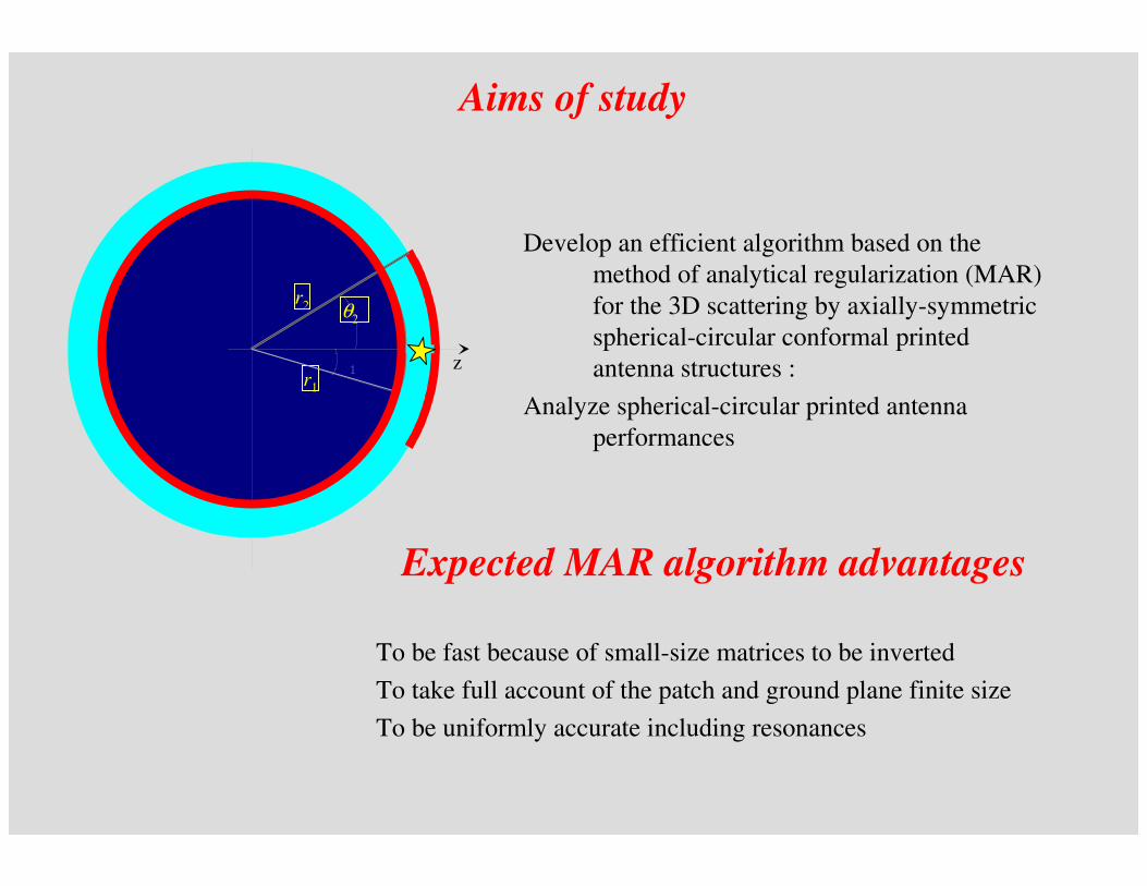
Develop an efficient algorithm based on the
method of analytical regularization (MAR)
for the 3D scattering by axially-symmetric
spherical-circular conformal printed
antenna structures :
Analyze spherical-circular printed antenna
performances
Aims of study
To be fast because of small-size matrices to be inverted
To take full account of the patch and ground plane finite size
To be uniformly accurate including resonances
Expected MAR algorithm advantages
r1
r2 θ2
z

Disadvantages of other approaches not based on
analytical regularization
FDTD and MoM fail near
the natural frequencies
because of staircasing and
lack of convergence
MAR guarantees high
accuracy even near the
high-Q natural frequencies
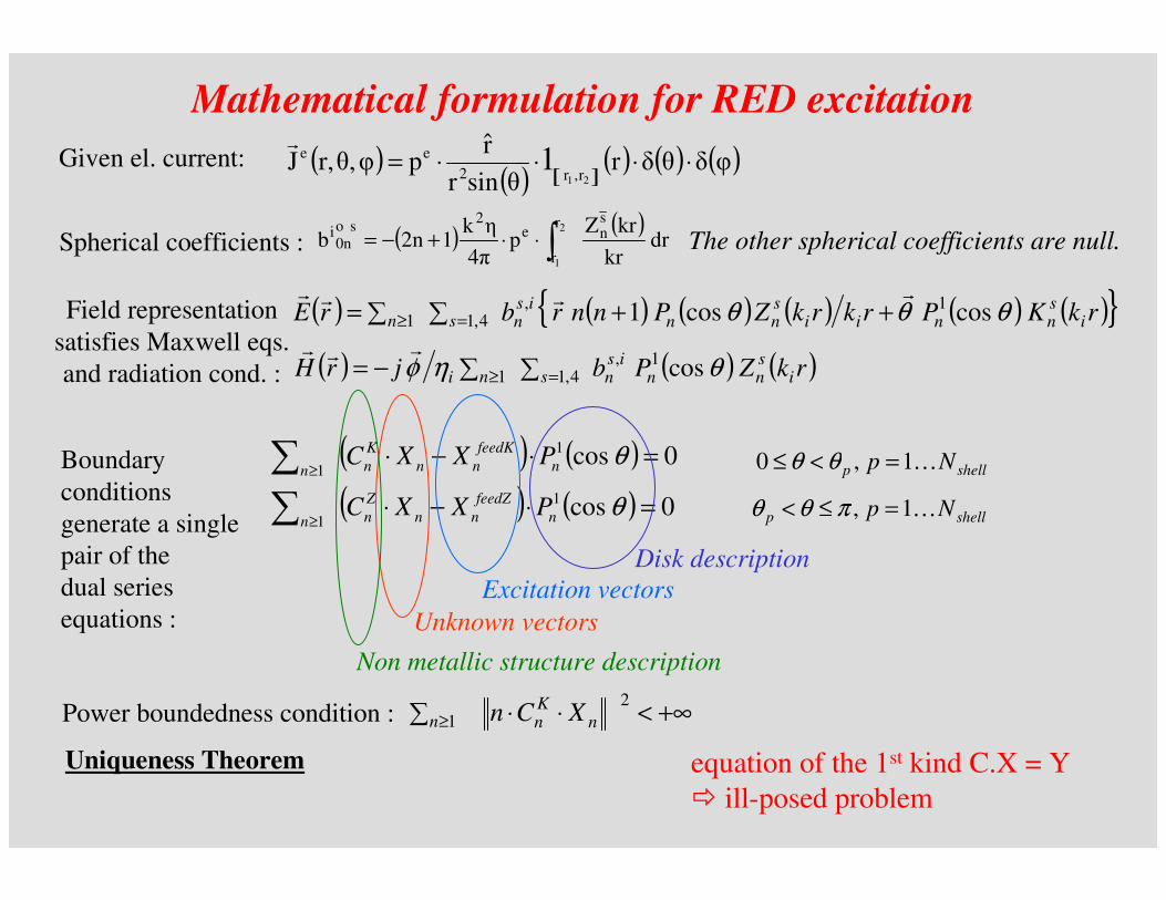
Mathematical formulation for RED excitation
( )( ) [ ]
( ) ( ) ( )φδθδrθsinr
r̂pφθ,r,J
21 r,r2
ee 1 ⋅⋅⋅⋅=�
Given el. current:
( ) ( )dr
kr
krZp
4π
ηk12nb
sn
r
r
e2
s o0n
i 2
1∫⋅⋅+−= The other spherical coefficients are null.Spherical coefficients :
( ) ( ) ( ) ( ) ( ) ( ){ }rkKPrkrkZPnnrbrE isnnii
snn
isnsn θθθ coscos1 1,
4,11
�
��
�
++∑∑= =≥
( ) ( ) ( )rkZPbjrH isnn
isnsni θηφ cos1,
4,11 ∑∑−= =≥
�
�
�
Field representation
satisfies Maxwell eqs.
and radiation cond. :
Boundary
conditions
generate a single
pair of the
dual series
equations :
( ) ( ) 0cos1
1=⋅−⋅∑ ≥
θn
feedK
nn
K
nnPXXC
( ) ( ) 0cos1
1=⋅−⋅∑ ≥
θn
feedZ
nn
Z
nnPXXC
shellp Np …1,0 =<≤ θθ
shellp Np …1, =≤< πθθ
Excitation vectors
Unknown vectors
Non metallic structure description
Disk description
Power boundedness condition : +∞<⋅⋅∑ ≥
2
1 nKnn XCn
Uniqueness Theorem equation of the 1st kind C.X = Y
� ill-posed problem
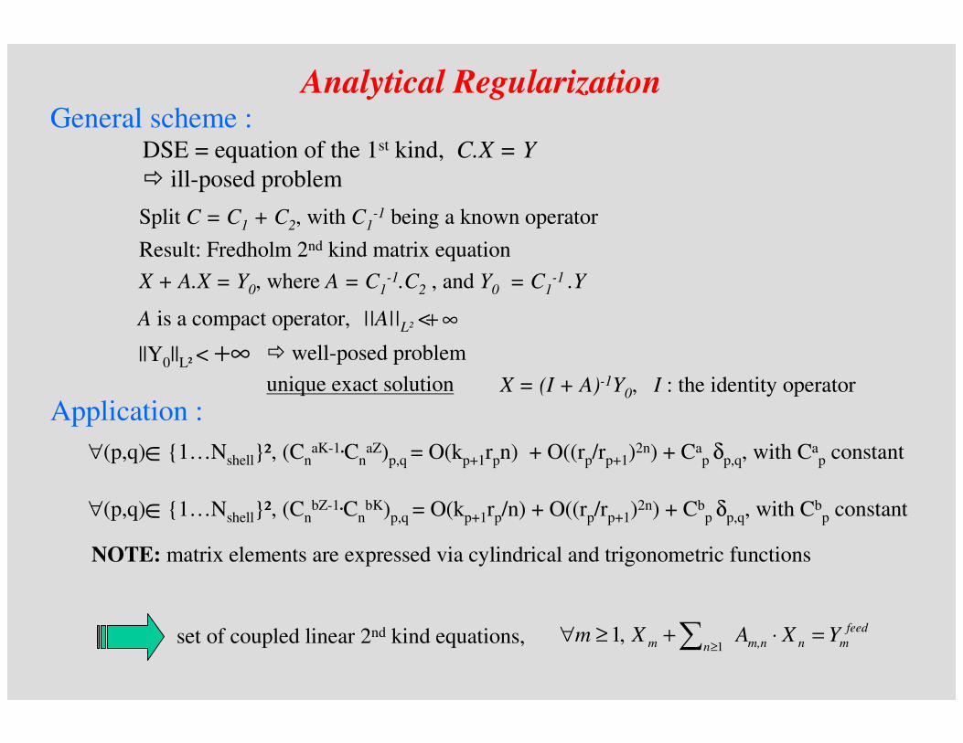
Analytical RegularizationGeneral scheme :
Split C = C1 + C2, with C1-1 being a known operator
A is a compact operator, ||A||L² <
X + A.X = Y0, where A = C1-1.C2 , and Y0 = C1
-1 .Y
Result: Fredholm 2nd kind matrix equation
∞+
||Y0||L² < ∞+unique exact solution X = (I + A)-1Y0, I : the identity operator
� well-posed problem
Application :
NOTE: matrix elements are expressed via cylindrical and trigonometric functions
DSE = equation of the 1st kind, C.X = Y
� ill-posed problem
∀(p,q) {1…Nshell}², (CnaK-1.Cn
aZ)p,q = O(kp+1rpn) + O((rp/rp+1)2n) + Ca
p δp,q, with Cap constant∈
∀(p,q) {1…Nshell}², (CnbZ-1.Cn
bK)p,q = O(kp+1rp/n) + O((rp/rp+1)2n) + Cb
p δp,q, with Cbp constant∈
set of coupled linear 2nd kind equations, feed
mnm,nnm YXAXm =⋅+≥∀ ∑ ≥1,1

Algorithm properties
Algorithm convergence rate is examined by plotting the relative error er(N) in the L2² norme :
( )²
N
²
1-NN
r
2
2
X
XXNe
L
L−
=
For a d-digit accuracy, take N = max|krmax| + Const d.(rmax/h) + 5
Typically, N < 120 for standard studies � Inversion of a small well-posed linear system
� Low CPU time & memory capacity consuming
Truncate at order N �
AAlimN
N
=+∞→
as ( ) 0NelimN
=+∞→�
Finite-size matrix equation � XN + AN.XN = Y0N
( ) ( )22 L
N
L
1
N
AAAIX
XXNe −⋅+≤
−=
−
,1 Nm ≤≤

Application to SCMA study, centered RED feeding
Very fast algorithm: far field computation time
- 1s with non optimized MAR-based program,
per frequency point
- 16h41m with HFSS 8 software (kr2=0.75 to 10,
fast sweep option with 3 frequency points, 41389 cells)
- problems of convergence with CST 3 µwave
Studio software
θ1 = 180°, θ2 = 18°, r1/r2 = 0.97
εr1 = εr3=1, εr2 = 1.3
µr1 = µr2 = µr3 = 1
0 50 100 150 20010
-6
10-4
10-2
100
102
k.r2=4
k.r2=10
k.r2=20
k.r2=30
k.r2=50
k.r2=75
k.r2=95
Order of truncation N
er(N)
Convergence, error(N)
r1
r2 θ2
z

Application to SCMA study, centered RED feeding
Effect of éléments of spherical-ground SCMA on the input resistance
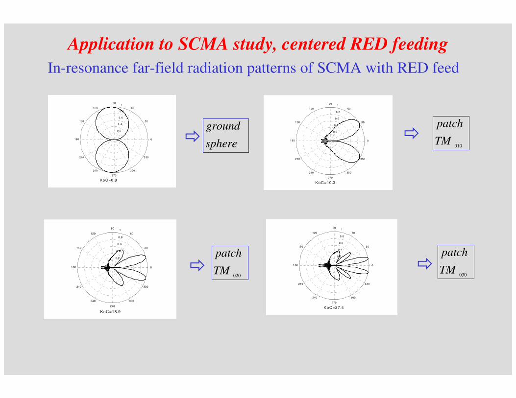
Application to SCMA study, centered RED feeding
In-resonance far-field radiation patterns of SCMA with RED feed
0.2
0.4
0.6
0.8
1
30
210
60
240
90
270
120
300
150
330
180 0
KoC=0.8
0.2
0.4
0.6
0.8
1
30
210
60
240
90
270
120
300
150
330
180 0
KoC=10.3
0.2
0.4
0.6
0.8
1
30
210
60
240
90
270
120
300
150
330
180 0
KoC=18.9
0.2
0.4
0.6
0.8
1
30
210
60
240
90
270
120
300
150
330
180 0
KoC=27.4
010TM
patch
�
�
�
�030
TM
patch
sphere
ground
020TM
patch

Application to SCMA study, centered RED feeding
Effect of each element of SCMA on the directivity
The ground improves the directivity�
θ2 = 18°,
r1/r2 = 0.97,
εr1 = εr3= 1.00,
εr2 = 1.30
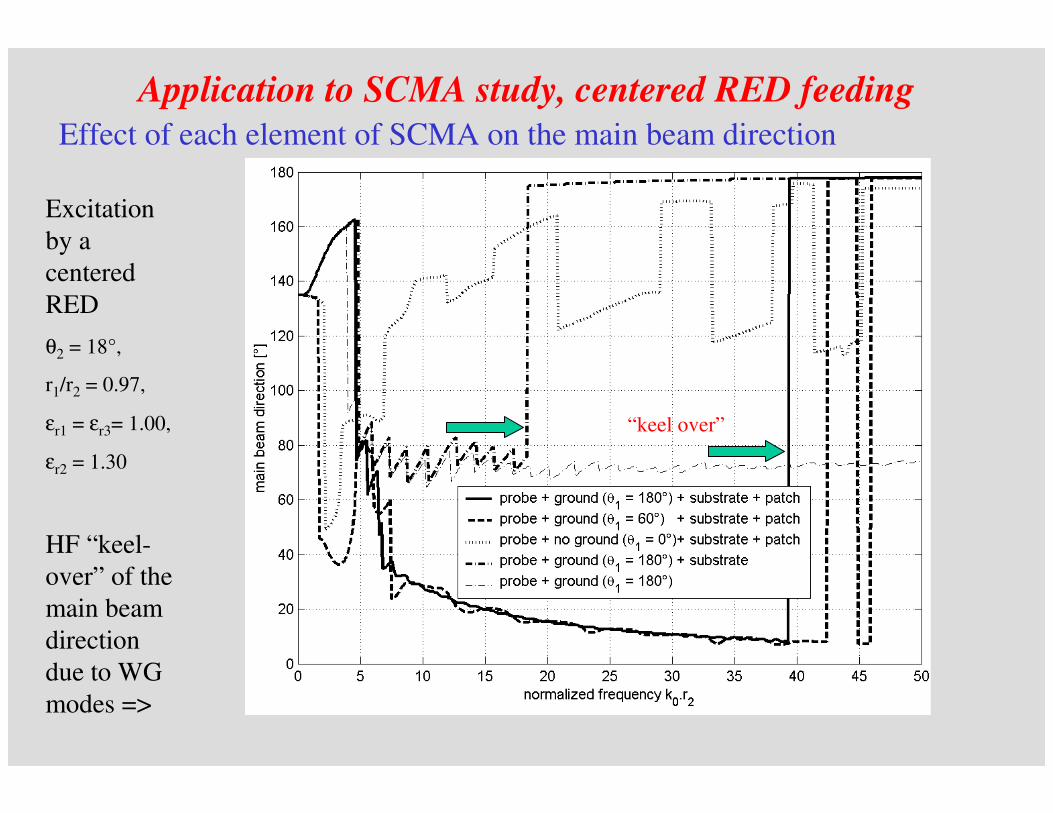
Application to SCMA study, centered RED feeding
Effect of each element of SCMA on the main beam direction
Excitation
by a
centered
RED
θ2 = 18°,
r1/r2 = 0.97,
εr1 = εr3= 1.00,
εr2 = 1.30
HF “keel-
over” of the
main beam
direction
due to WG
modes =>
“keel over”
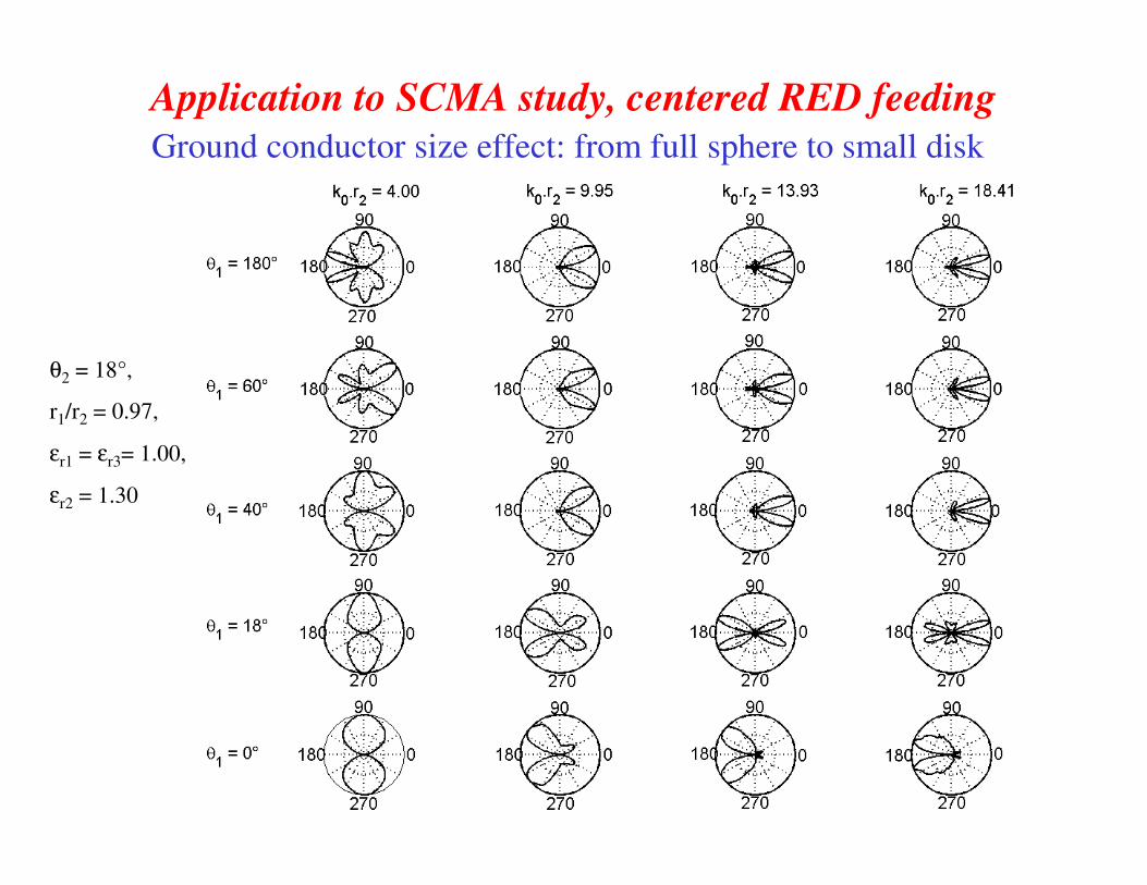
Application to SCMA study, centered RED feeding
Ground conductor size effect: from full sphere to small disk
θ2 = 18°,
r1/r2 = 0.97,
εr1 = εr3= 1.00,
εr2 = 1.30
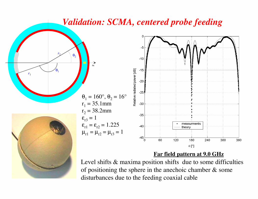
Validation: SCMA, centered probe feeding
θ1 = 160°, θ2 = 16°
r1 = 35.1mm
r2 = 38.2mm
εr3 = 1
εr1 = εr2 = 1.225
µr1 = µr2 = µr3 = 1
r1
r2 θ2
z
Far field pattern at 9.0 GHz
Level shifts & maxima position shifts due to some difficulties
of positioning the sphere in the anechoic chamber & some
disturbances due to the feeding coaxial cable
θ1
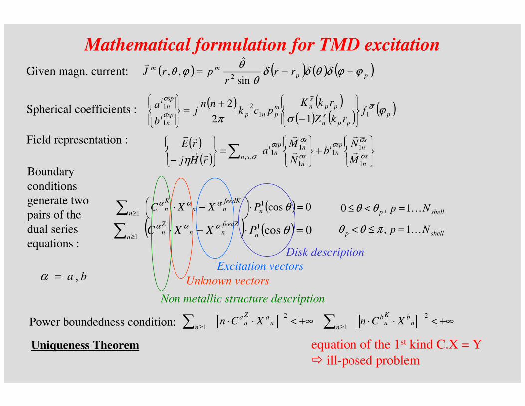
Mathematical formulation for TMD excitation
( )( )
+
=
−∑ s
n
snsp
ni
sn
snsp
ni
sn M
Nb
N
Ma
rHj
rEσ
σσ
σ
σσ
ση 1
11
1
11
,,�
�
�
�
�
�
�
�
Field representation :
Uniqueness Theorem equation of the 1st kind C.X = Y
� ill-posed problem
Given magn. current: ( ) ( ) ( ) ( )ppmm rr
rprJ ϕϕδθδδ
θ
θϕθ −−=
sin
ˆ,,
2
�
Spherical coefficients :( ) ( )
( ) ( ) ( )p
ppsn
ppsnm
pnpsp
ni
sp
ni
frkZ
rkKpck
nnj
b
aϕ
σπσ
σ
σ
11
2
1
1
12
2
−
+=
Boundary
conditions
generate two
pairs of the
dual series
equations :
( ) 0cos1
1=⋅
−⋅∑ ≥
θαααn
feedK
nn
K
nn
PXXC
( ) ( ) 0cos1
1=⋅−⋅∑ ≥
θαααn
feedZ
nn
Z
nn
PXXC
shellp Np …1,0 =<≤ θθ
shellp Np …1, =≤< πθθ
Excitation vectors
Unknown vectors
Non metallic structure description
Disk description
ba ,=α
Power boundedness condition: +∞<⋅⋅∑ ≥
2
1n
aZ
na
nXCn +∞<⋅⋅∑ ≥
2
1n
bK
nb
nXCn
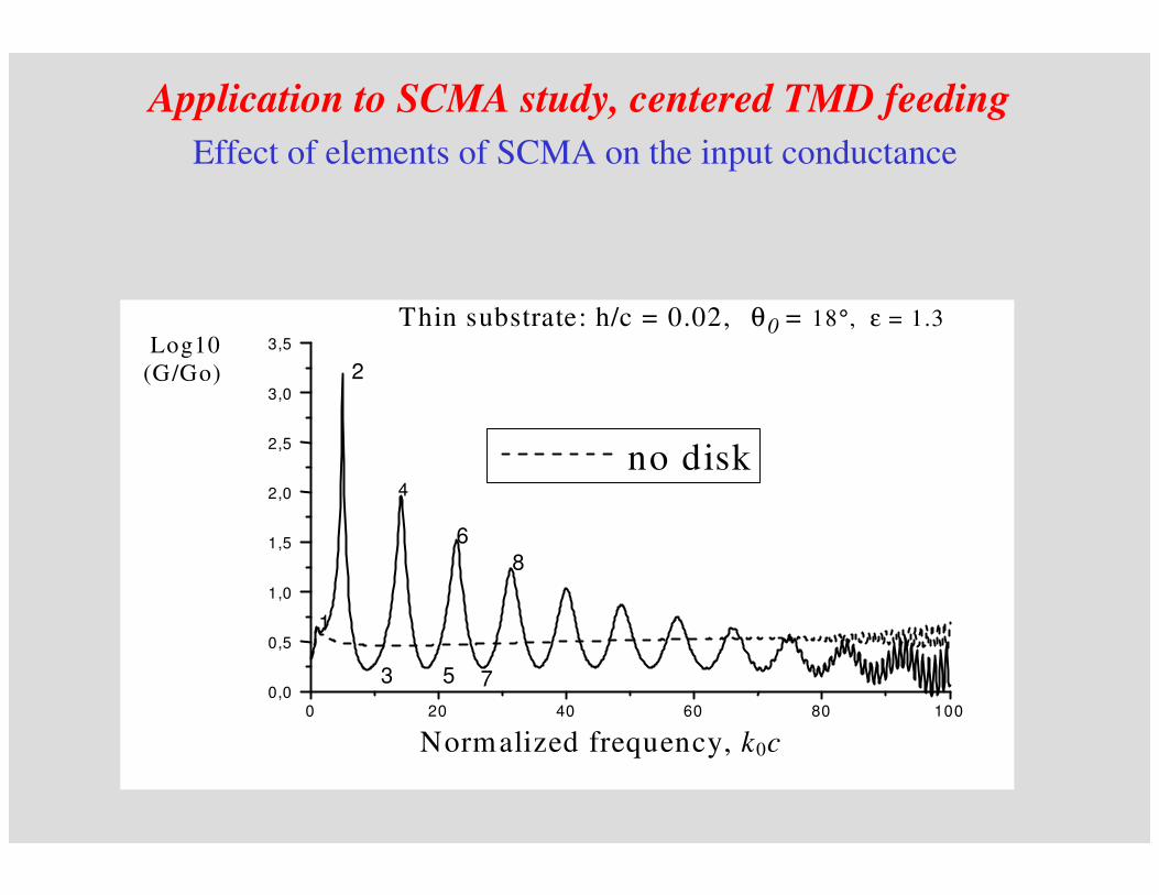
Application to SCMA study, centered TMD feeding
Effect of elements of SCMA on the input conductance
Thin substrate: h/c = 0.02, 0θ = 18°, ε = 1.3
0 20 40 60 80 100 0,0
0,5
1,0
1,5
2,0
2,5
3,0
3,5
Log10
(G/Go)
Normalized frequency, k0c
no disk
1
2
3
4
5
6
7
8

Application to SCMA study, centered TMD feeding
In-resonance far-field radiation pattern of SCMA with TMD feed
0.2
0.4
0.6
0.8
1
30
210
60
240
90
270
120
300
150
330
180 0
KoC= 1 a/c= 0.98 To=18° ep=1.3
fi=0°
fi=90°
0.2
0.4
0.6
0.8
1
30
210
60
240
90
270
120
300
150
330
180 0
K oC=5 a/c=0.98 To= 18° ep= 1.3
fi= 0°
fi= 90°
0.2
0.4
0.6
0.8
1
30
210
60
240
90
270
120
300
150
330
180 0
KoC=14.2 a/c=0.98 To=18° ep=1.3
fi=0°
fi=90°
0.2
0.4
0.6
0.8
1
30
210
60
240
90
270
120
300
150
330
180 0
KoC=22.8 a/c=0.98 To=18° ep=1.3
fi=0°
fi=90°
120qTM
patch
130qTM
patch
sphere
ground
110qTM
patch
�
� �
�

Application to SCMA study, centered TMD feeding
Effect of elements of SCMA on the directivity of radiation
0 5 10 15 20 25 30 35 40 45 50 0
5
10
15
20
25
30
35
40
Normalized frequency, k0c
D - - - no disk

Application to SCMA study, centered TMD feeding
Effect of elements of SCMA on the main beam direction
0 5 10 15 20 25 30 35 40 45 50 0
20
40
60
80
100
120
140
160
180
Normalized frequency, k0c
Θmax - - - no disk
“keel over”

Conclusions
MAR-based simulation is a very fast and accuratemethod to study SCMA radiation and related problems.
This study :
- highlights effects of the ground conductor size and curvature,
- reveals several types of resonances connected with patch,
ground, and dielectric substrate,
- reveals the effect of the ”keel over” of the main radiation beam
at high frequencies
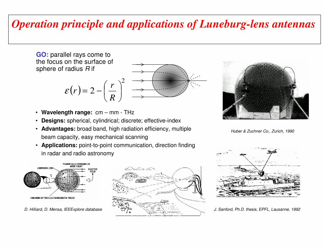
Operation principle and applications of Luneburg-lens antennas
( )2
2
−=
R
rrε
GO: parallel rays come to the focus on the surface of sphere of radius R if
• Wavelength range: cm – mm - THz
• Designs: spherical, cylindrical; discrete; effective-index
• Advantages: broad band, high radiation efficiency, multiple
beam capacity, easy mechanical scanning
• Applications: point-to-point communication, direction finding
in radar and radio astronomy
J. Sanford, Ph.D. thesis, EPFL, Lausanne, 1992D. Hilliard, D. Mensa, IEEExplore database
Huber & Zuchner Co., Zurich, 1990
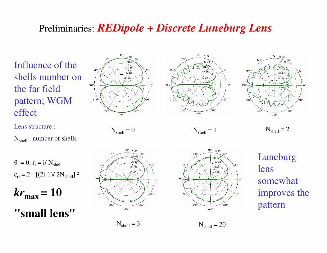
Preliminaries: REDipole + Discrete Luneburg Lens
Nshell = 3 Nshell = 20
Nshell = 0 Nshell = 1 Nshell = 2
Luneburg
lens
somewhat
improves the
pattern
Influence of the
shells number on
the far field
pattern; WGM
effect
Lens structure :
Nshell : number of shells
θi = 0, ri = i/ Nshell
εri = 2 - [(2i-1)/ 2Nshell] ²
krmax = 10
"small lens"

Preliminaries: TMDipole + Discrete Luneburg Lens
Influence of the
shells number on
the far field
pattern; WGM
effect
Lens structure :
Nshell : number of
shells
krmax = 10
"small lens"
εri = 2- [(2i-1)/ 2Nshell] ²
N=3N=0
N=1
N=2
N=20
Luneburg lens
improves pattern,
however not
dramatically
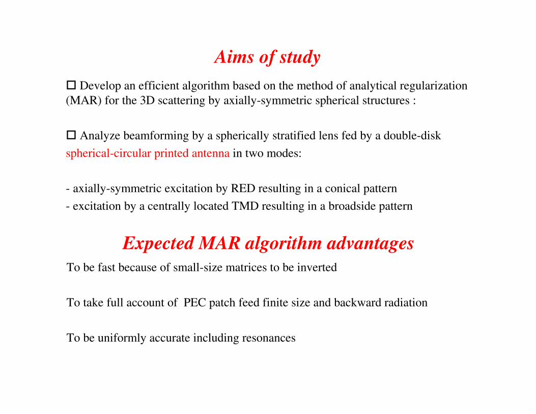
� Develop an efficient algorithm based on the method of analytical regularization
(MAR) for the 3D scattering by axially-symmetric spherical structures :
� Analyze beamforming by a spherically stratified lens fed by a double-disk
spherical-circular printed antenna in two modes:
- axially-symmetric excitation by RED resulting in a conical pattern
- excitation by a centrally located TMD resulting in a broadside pattern
Aims of study
To be fast because of small-size matrices to be inverted
To take full account of PEC patch feed finite size and backward radiation
To be uniformly accurate including resonances
Expected MAR algorithm advantages

Analyzed geometry: Dipole + SCMA + DLL
1
Nshell
Nshell +1
rNshell
θin
2
...
Conformal patches
Lens: concentric
spherical layers
of dielectrics
Patches: PEC,
zero-thickness,
co-axially placed
spherical disks,
0≤θ ≤π
θoutGiven driving
current:
centered
RED or
TMD,
as a probe or
a slot model
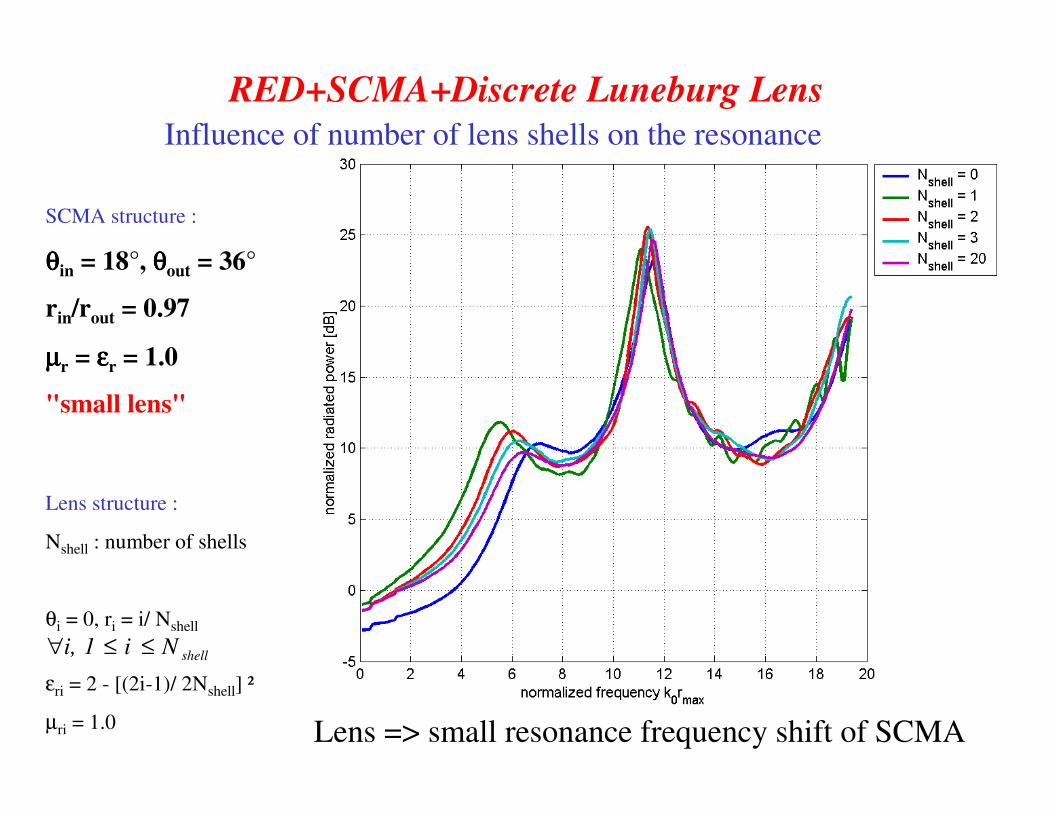
RED+SCMA+Discrete Luneburg Lens
Influence of number of lens shells on the resonance
SCMA structure :
θθθθin = 18°, θθθθout = 36°
rin/rout = 0.97
µµµµr = εεεεr = 1.0
"small lens"
Lens => small resonance frequency shift of SCMA
Lens structure :
Nshell : number of shells
θi = 0, ri = i/ Nshell
εri = 2 - [(2i-1)/ 2Nshell] ²
µri = 1.0
shellNi1i, ≤≤∀
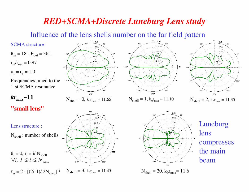
RED+SCMA+Discrete Luneburg Lens study
Influence of the lens shells number on the far field pattern
SCMA structure :
θin = 18°, θout = 36°,
rin/rout = 0.97
µr = εr = 1.0
Frequencies tuned to the
1-st SCMA resonance
krmax~11
"small lens"
Nshell = 3, k0rmax = 11.45 Nshell = 20, k0rmax= 11.6
Nshell = 0, k0rmax = 11.65 Nshell = 1, k0rmax = 11.10 Nshell = 2, k0rmax = 11.35
Luneburg
lens
compresses
the main
beam
Lens structure :
Nshell : number of shells
θi = 0, ri = i/ Nshell
εri = 2 - [(2i-1)/ 2Nshell] ²
shellNi1i, ≤≤∀
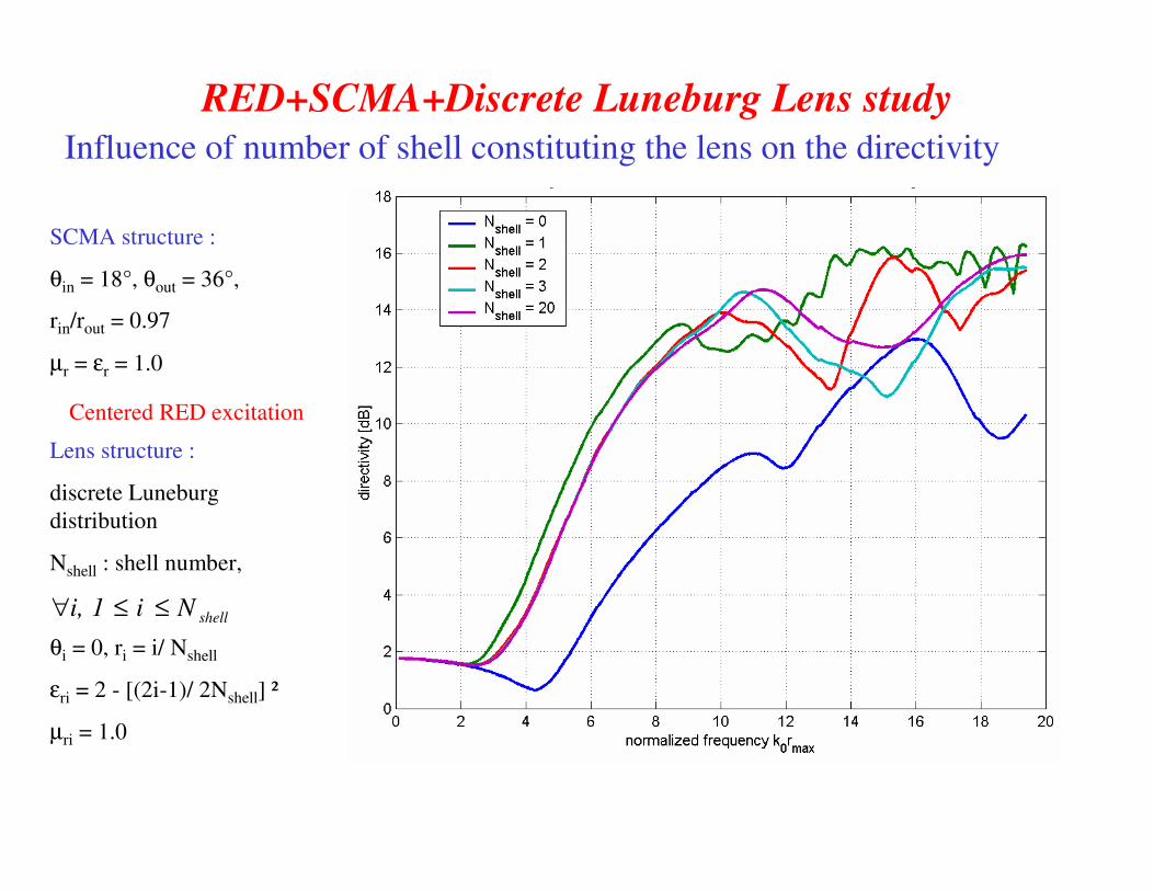
RED+SCMA+Discrete Luneburg Lens study
Influence of number of shell constituting the lens on the directivity
SCMA structure :
θin = 18°, θout = 36°,
rin/rout = 0.97
µr = εr = 1.0
Lens structure :
discrete Luneburg
distribution
Nshell : shell number,
θi = 0, ri = i/ Nshell
εri = 2 - [(2i-1)/ 2Nshell] ²
µri = 1.0
shellNi1i, ≤≤∀
Centered RED excitation

RED+SCMA+Discrete Luneburg Lens study
Influence of number of lens shells on the resonance; WGM effect
SCMA structure :
θin = 0.02°,
θθθθout = 0.04°
rin/rout = 0.999
"large lens"
Lens => small shift in SCMA resonance frequencies
Lens structure :
Nshell : number of shells
θi = 0, ri = i/ Nshell
εri = 2 - [(2i-1)/ 2Nshell] ²
shellNi1i, ≤≤∀
TM010 TM011

REDipole+Discrete Luneburg Lens Radiation
N=0
N=1
Uniform
dielectric
sphere
significantly
improves
far-field
radiation
pattern,
however
WGM
sidelobes
appear
TM010: krmax=53 TM011: krmax=97.6
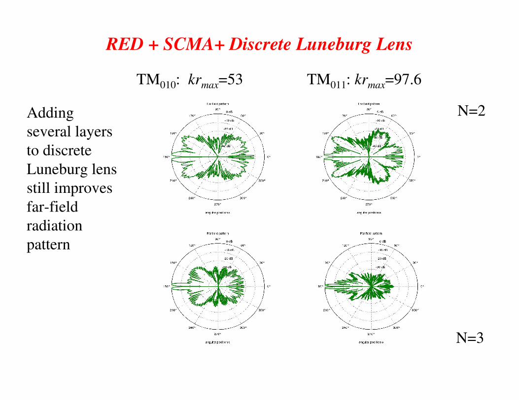
RED + SCMA+ Discrete Luneburg Lens
N=2
N=3
Adding
several layers
to discrete
Luneburg lens
still improves
far-field
radiation
pattern
TM010: krmax=53 TM011: krmax=97.6
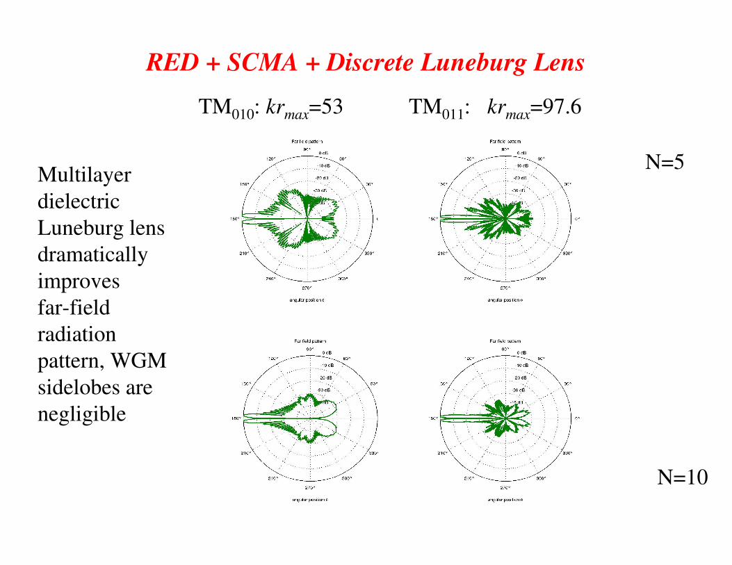
RED + SCMA + Discrete Luneburg Lens
N=5
N=10
Multilayer
dielectric
Luneburg lens
dramatically
improves
far-field
radiation
pattern, WGM
sidelobes are
negligible
TM011: krmax=97.6TM010: krmax=53

Validation: RED + SCMA + DLL
centered coaxial probe feeding
θin = 2.0°, θout = 4.0°
rNshell-1 = 99% rNshell
εrNshell = 1
k0 rNshell = 20.94 (f = 5.0GHz)
Very good agreement between theory and
measurements
Nshell
rNshell
θin
...
θout
Eccostok Luneberg lens-P16©
(Emerson & Cuming)
theorymeasurements

TMD+SCMA+Discrete Luneburg Lens study
Influence of the lens shells number on the far field pattern
Lens
compresses
the beam
Lens structure :
discrete Luneburg
distribution
Nshell = 40 shells
θi = 0, ri = i/ Nshell
εri = 2 - [(2i-1)/ 2Nshell] ²
µri = 1.0
shellNi1i, ≤≤∀
θθθθin = 1.3°, θθθθout = 3°,
rin/rout = 0.97
µµµµr = εεεεr = 1.0
k0rmax = 10
"small lens"

TMD+SCMA+Discrete Luneburg Lens study
Influence of number of lens shells on the resonance; WGM effect
SCMA structure :
θθθθin = 0.02°,
θθθθout = 0.04°
rin/rout = 0.999
"large lens"
Lens => small resonance frequency shift of SCMA
Lens structure :
Nshell : number of shells
θi = 0, ri = i/ Nshell
εri = 2 - [(2i-1)/ 2Nshell] ²
shellNi1i, ≤≤∀
qTM110

TMD + SCMA + Discrete Luneburg Lens
N=0
N=1
Uniform
dielectric
sphere
significantly
improves
far-field
radiation
pattern
krmax=69
"large lens"

TMD + SCMA + Discrete Luneburg Lens
N=2
N=3
Several-layer
dielectric
Luneburg lens
still improves
far-field
radiation
pattern,
however not
much
krmax=69
"large lens"

Validation: TMD + SCMA + DLL
centered slot feedingNshell
rNshell
θin
...
θout
Eccostok Luneberg lens-P16©
(Emerson & Cuming)
θin = 2.0°, θout = 4.0°
rNshell-1 = 99% rNshell
εrNshell = 1
k0 rNshell = 25.5 (f = 6 GHz)
E-plane
H-plane
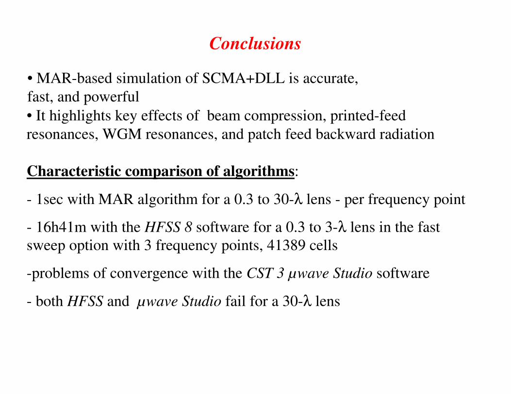
Conclusions
• MAR-based simulation of SCMA+DLL is accurate,
fast, and powerful
• It highlights key effects of beam compression, printed-feed
resonances, WGM resonances, and patch feed backward radiation
Characteristic comparison of algorithms:
- 1sec with MAR algorithm for a 0.3 to 30-λ lens - per frequency point
- 16h41m with the HFSS 8 software for a 0.3 to 3-λ lens in the fast
sweep option with 3 frequency points, 41389 cells
-problems of convergence with the CST 3 µwave Studio software
- both HFSS and µwave Studio fail for a 30-λ lens

Microwave power absorption in a partially screened
two-layer lossy dielectric sphere
Boundary-value problem:
1. Maxwell equations
2. Boundary conditions
3. Edge condition
4. Radiation condition
(1)
0
1
' (1) (1)
2 0 0 0 0 0
1 1
( )
1(1 ) (2 1) ( ) ( ) ( ) ( 1) ( )
2
m n nm n m
n
m
m n n nm n n nm
n n
X Q X V
V k c n k b k c Q n n Q
ε θ
ε ζ ψ θ α δ θ
∞
=
∞ ∞
= =
= +
= + + + + −
∑
∑ ∑
Final result of analytical
regularization:
Geometry: layered sphere axisymmetrically
excited by a Radial Electric Dipole (RED)
θ
a
0
c
b
2ε1ε
RED as antenna

Bone:
thickness 2 mm
Brain:
radius 100 mm
Skin:
thickness 1 mm
f = 900 MHz f = 1500 MHz
52.7rε =
9.67rε =
59.1rε =
0.0508 /Сим мσ =
7.75rε =
0.105 /Сим мσ =
1.05 /Сим мσ = 1.65 /Сим мσ =
46.0rε =
1.26 /Сим мσ =
45.6rε =
1.93 /Сим мσ =
02
r
i
f
σε ε ε
π= +
Averaged electrophysical parameters of the
human head tissues
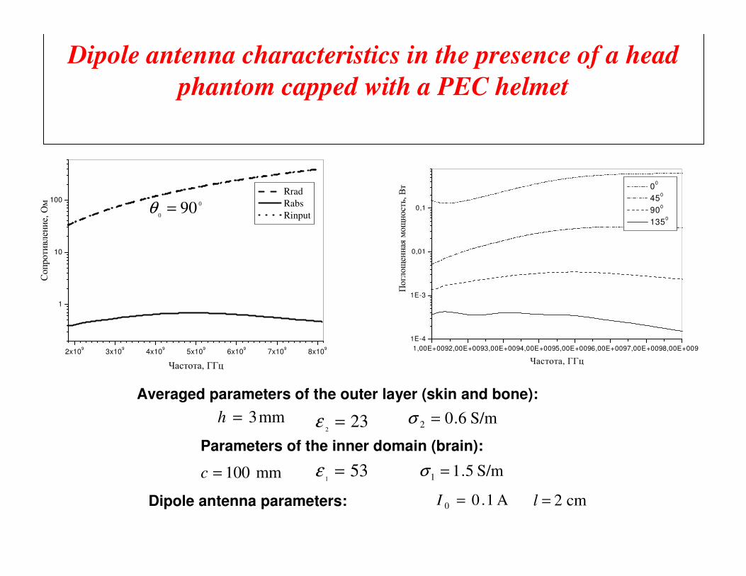
Dipole antenna characteristics in the presence of a head
phantom capped with a PEC helmet
2x10⁹
3x10⁹
4x10⁹
5x10⁹
6x10⁹
7x10⁹
8x10⁹
1
10
100 Rrad
Rabs
Rinput
Соп
роти
влен
ие, Ом
Частота, ГГц
1,00E+0092,00E+0093,00E+0094,00E+0095,00E+0096,00E+0097,00E+0098,00E+009
1E-4
1E-3
0,01
0,1
Пог
лощен
ная мощ
ность,
Вт
Частота, ГГц
00
450
900
1350
531
=ε
232
=ε
A1.00 =I cm2=l
S/m5.11 =σ
S/m6.02 =σ
mm100=c
mm3=h
0
090=θ
Averaged parameters of the outer layer (skin and bone):
Parameters of the inner domain (brain):
Dipole antenna parameters:
0 20 40 60 80 100 120 140 160 18010
-10
10-8
10-6
10-4
10-2
100
Угловой размер, градусы
Поглощенная мощность, Вт
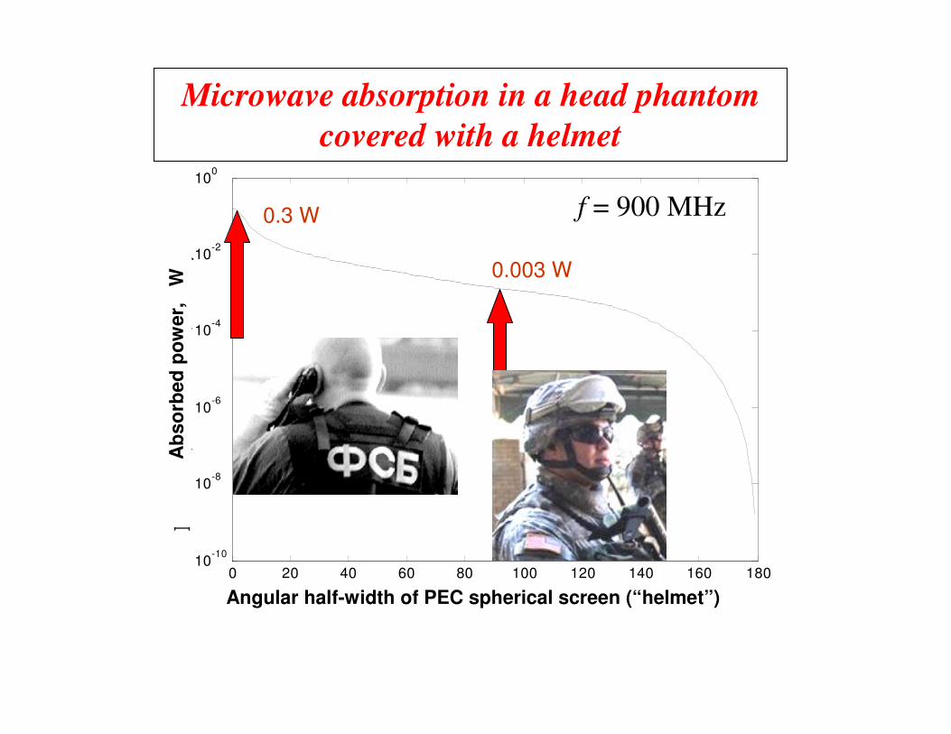
Microwave absorption in a head phantom
covered with a helmet
0.003 W
0.3 W
Angular half-width of PEC spherical screen (“helmet”)
f = 900 MHz
Ab
so
rbe
d p
ow
er,
W
Conclusions
It has been shown that
• Metal hemispherical helmet can reduce EM absorption in
the head phantom in 100 times at the mobile-
communication frequencies
• No absorption resonances in the head phantom take place
in the presence of helmet, due to high conductivity values
of tissues