radiative transfer modeling in vegetation - earth online · radiative transfer modeling in...
TRANSCRIPT

1Envisat Summer School – NG 1
Nadine Gobron
With collaborations of:Bernard Pinty, Michel Verstraete & Jean-Luc Widlowski
Radiative Transfer Modeling in Vegetation

2Envisat Summer School – NG 1
Outline
• Scientific Problems with Space Remote Sensing
• Radiative Transfer Equations• Radiative Transfer Modeling for vegetation
canopy • RAMI • Conclusion

3Envisat Summer School – NG 1
Outline
• Scientific Problems with Space Remote Sensing
• Radiative Transfer Equations• Radiative Transfer Modeling for vegetation
canopy • RAMI • Conclusion

4Envisat Summer School – NG 1
What is the main scientific issue in remote sensing?
• Remote sensing instruments on space platforms are sophisticated detectors recording the occurrence of elementary events (the absorption of photons or electromagnetic waves) as variations in electrical currents or voltages.
• Users, on the other hand, require information on events and processes occurring in the geophysical environment (e.g., atmospheric pollution, oceanic currents, terrestrial net productivity, etc.)

5Envisat Summer School – NG 1 Source: Goscinny & Uderzo,1971, Hachette
DEFORESTATION

6Envisat Summer School – NG 1
REFORESTATION
Source: Goscinny & Uderzo,1971, Hachette

7Envisat Summer School – NG 1
AFFORESTATION
Source: Goscinny & Uderzo,1971, Hachette

8Envisat Summer School – NG 1
What is the main scientific issue in remote sensing?
• Remote sensing instruments on space platforms are sophisticated detectors recording the occurrence of elementary events (the absorption of photons or electromagnetic waves) as variations in electrical currents or voltages.
• Users, on the other hand, require information on events and processes occurring in the geophysical environment (e.g., atmospheric pollution, oceanic currents, terrestrial net productivity, etc.)
• Extracting useful environmental information from data acquired in space is the main challenge facing remote sensing scientists.

9Envisat Summer School – NG 1
How is remote sensing exploited?
• The signals detected by the sensors are immediately converted into digital numbers and transmitted to dedicated receiving stations, where these data are heavily processed.
• The effective exploitation of remote sensing data to reliably generate useful, pertinent information hinges on the availability and performance of specific tools and techniques of data analysis and interpretation.
• A variety of mathematical models can be used for this purpose; they are implemented as computer codes that read the data or intermediary products and ultimately lead to the generation of products and services usable in specific applications…. User is happy !

10Envisat Summer School – NG 1
Why is remote sensing called an inverse problem?
• Since space borne instruments can only measure the properties of electromagnetic waves emitted or scattered by the Earth, scientists need first to understand where these waves originate from, how they interact with the environment, and how they propagate towards the sensor.
• To this effect, they develop models of radiation transfer, assuming that everything is known about the sources of radiation and the environment, and calculate the properties of the radiation field as the sensor should measure them. This is the so-called direct problem.

11Envisat Summer School – NG 1
Why is remote sensing called an inverse problem?
• In practice, one does acquire the measurements from the satellite, and would like to know what is going on in the environment:
à This is the inverse problem, which is much more complicated: Knowing the value of the electromagnetic measurements gathered in space, how can we derive the properties of the environment that were responsible for the radiation to reach the sensor?
12Envisat Summer School – NG 1
Radiative Transfer Modeling • In solar domain, radiation transfer models are tools to
represent the scattering and absorption of radiation by scattering elements/centers. They should satisfy energy conservation.
• Spectral properties are depending on the geophysical medium: atmosphere, ocean, soil, or vegetation
• Monograph dealing with RT problems in geophysics (Chandrasekhar (1960), Van de Hulst (1957), Lenoble(1993), Hapke (1993), Liou (1980) etc…) mainly concentrate on mathematical issues related to solving equations.
• Rather than discussing the solving of approximate equations applicable to realistic geophysical situations, we will concentrate on exact and light mathematical treatment of a simplified physical system…
Definition in Radiative Transfer Modeling

13Envisat Summer School – NG 1
Outline
• Scientific Problems with Space Remote Sensing
• Radiative Transfer Equations• Radiative Transfer Modeling for vegetation
canopy • RAMI • Conclusion

14Envisat Summer School – NG 1
Radiative Transfer Equations (1)
• Exact and light mathematical treatment of a simplified physical system
• The system under consideration will have the following properties:
– A continuous scattering-absorbing medium, infinite in lateral extent, bounded by two parallel planes, i.e. a plane-parallel medium.
– Radiation can be scattered in only two directions, upward and downward.
Radiative Transfer Equations
z=0
z
z+∆z
z=zh

15Envisat Summer School – NG 1
• The system under consideration will have the following properties:– Radiation or “ensemble of photons” is emitted by sources outside the
medium only.– The amount of mean monochromatic radiant energy traveling upward
and downward that crosses a unit area per unit time is an intensity noted I [Wm-2sr-1].
Radiative Transfer Equations
I (z)
I (z+∆z) I (z+∆z)
I (z)
z=0
z
z+∆z
z=zh
Radiative Transfer Equations (1)

16Envisat Summer School – NG 1
Scattering“A physical process by which an ensemble of particles immerged into an electromagnetic radiation field remove energy from the incident waves to re-irradiate this energy into other directions”
Absorption“A physical process by which an ensemble of particles immerged into an electromagnetic radiation field remove energy from the incident waves to convert this energy in a different form”
Extinction“A physical process by which an ensemble of particles immerged into an electromagnetic radiation field remove energy from the incident waves to attenuate the energy of this incident wave”
Basic Processes (1)
Radiative Transfer Equations

17Envisat Summer School – NG 1
Basic Processes (2)
•The upward and downward intensities change along the vertical coordinate z in the medium according to the volumetric (individual cross-sections times the number per unit volume) coefficients of absorption, K (in m-1) and scattering S (in m-1)
•Thus 1/S (1/K) have dimensions of length and may be interpreted as the absorption (scattering) mean free paths, i.e. the average distance between absorption (scattering) events.
Radiative Transfer Equations
I (z)
I (z+∆z) I (z+∆z)
I (z)
z=0
z
z+∆z
z=zh

18Envisat Summer School – NG 1
P is the probability that a photon directed upward is scattered downward
P is the probability that a photon directed downward is scattered upward
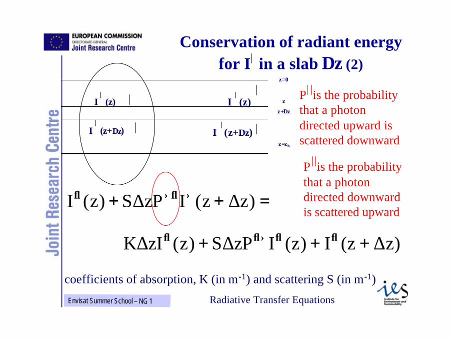
Conservation of radiant energyfor I in a slab ∆z (2)
z=0
z
z+∆z
z=zh
I (z)
I (z+∆z) I (z+∆z)
I (z)
=++ ↑↑↓↓ )zz(IzPS)z(I ∆∆
)zz(I)z(IzPS)z(zIK ∆∆∆ +++ ↓↓↓↑↓
coefficients of absorption, K (in m-1) and scattering S (in m-1)
Radiative Transfer Equations
19Envisat Summer School – NG 1
P is the probability that a photon directed upward is scattered downward
P is the probability that a photon directed downward is scattered upward
Conservation of radiant energyfor I in a slab ∆z (2)
z=0
z
z+∆z
z=zh
I (z)
I (z+∆z) I (z+∆z)
I (z)
=++ ↑↑↓↓ )zz(IzPS)z(I ∆∆
)zz(I)z(IzPS)z(zIK ∆∆∆ +++ ↓↓↓↑↓
coefficients of absorption, K (in m-1) and scattering S (in m-1)
Radiative Transfer Equations

20Envisat Summer School – NG 1
Conservation of radiant energy for I in a slab ∆z
z=0
z
z+∆z
z=zh
I (z)
I (z+∆z) I (z+∆z)
I (z)
=++ ↓↓↑↑ )z(IzPS)zz(I ∆∆
)z(I)zz(IzPS)zz(zIK ↑↑↑↓↑ ++++ ∆∆∆∆
Radiative Transfer Equations
coefficients of absorption, K (in m-1) and scattering S (in m-1)

21Envisat Summer School – NG 1
Conservation of radiant energy in a slab ∆z
)()()()()( zISPzISPzKIz
zIzzI ↑↑↓↓↓↑↓↓↓
+−−=∆
−∆+
)()()()(
zISPzISPzKIzzI ↑↑↓↓↓↑↓
↓
+−−=∂
∂
Dividing both sides by ∆z:
where I (z) decreases in the direction of increasing z
Radiative Transfer Equations
…. taking the limit as ∆zà 0 gives:

22Envisat Summer School – NG 1
Conservation of radiant energy in a slab ∆z
)z(ISP)z(ISP)z(KIz
)z(I ↑↑↓↓↓↑↓↓
+−−=∂
∂
)z(ISP)z(ISP)z(KIz
)z(I ↓↓↑↑↑↓↑↑
−++=∂
∂
We obtain the two-stream equations
Radiative Transfer Equations
coefficients of absorption, K (in m-1) and scattering S (in m-1)

23Envisat Summer School – NG 1
•We have for isotropic medium:
•The asymmetry factor g is a single number, defined as the mean cosine of the scattering angle (-1 or +1 in our case):
•Typically: g = +1 for strict downward scattering,
g=-1 for strict upward scattering and,
g=0 for isotropic scattering.
•For the above set of equations, we have:
Asymmetry factor for scattering processes
↓↑↑↓ = PP
↓↑↓↓ −++= P)1(P)1(g
2/)g1(PP
2/)g1(PP
+==
−==↓↓↑↑
↓↑↑↓
1PPPP =+=+ ↓↓↓↑↑↑↑↓
↑↑↓↓ = PP

24Envisat Summer School – NG 1
•Normalization of the radiation transport equations by the extinction factor E=S+K gives :
which can be rewritten as:
where is called the single scattering albedo
expressing the probability for the photons to be scattered.
Single scattering albedo
)z(IPES
)z(IPES
)z(IEK
z)z(I
E1 ↑↑↓↓↓↑↓
↓
+−−=∂
∂
)z(I2
)g1()z(I
2)g1(
)z(Iz
)z(IE1 ↑↓↓
↓ −+
++−=
∂∂
ωω
)z(I2
)g1()z(I
2)g1(
)z(Iz
)z(IE1 ↓↑↑
↑ −−
+−+=
∂∂
ωω
ES
KSS
=+
=ω
Radiative Transfer Equations

25Envisat Summer School – NG 1
• Single scattering albedo ω =0 for total absorption (no scattering)
• Single scattering albedo ω =1 for total or conservative scattering (no absorption)
Single scattering albedo
ES
KSS
=+
=ω
)z(I2
)g1()z(I
2)g1(
)z(Iz
)z(IE1 ↑↓↓
↓ −+
++−=
∂∂
ωω
)z(I2
)g1()z(I
2)g1(
)z(Iz
)z(IE1 ↓↑↑
↑ −−
+−+=
∂∂
ωω
Radiative Transfer Equations
26Envisat Summer School – NG 1
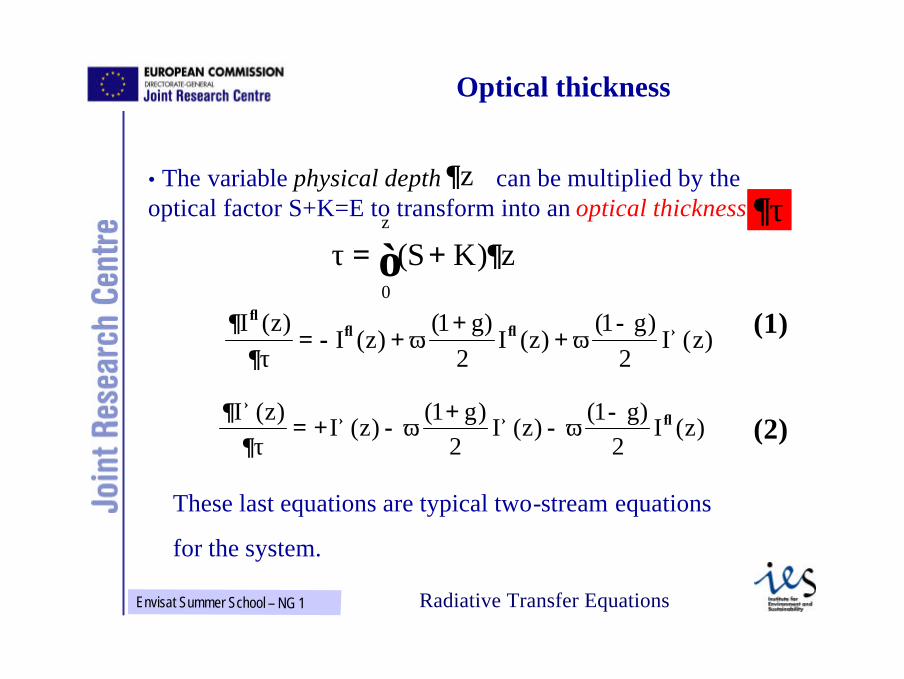
• The variable physical depth can be multiplied by the optical factor S+K=E to transform into an optical thickness
Optical thickness
)z(I2
)g1()z(I
2)g1(
)z(I)z(I ↑↓↓
↓ −+
++−=
∂∂
ωωτ
)z(I2
)g1()z(I
2)g1(
)z(I)z(I ↓↑↑
↑ −−
+−+=
∂∂
ωωτ
z∂τ∂
z)KS(z
0
∂+= ∫τ
These last equations are typical two-stream equations
for the system.
Radiative Transfer Equations
(1)
(2)

27Envisat Summer School – NG 1
• In a more compact form [with (1) - (2) and (1)+(2)]:
Two-stream equations
)II)(1()II( ↑↓
↑↓
+−−=∂−∂
ωτ
Key variables to represent the radiative transfer processes are:
• ω : the single scattering albedo
• g : the asymmetry factor of the phase function
• τ : the optical thickness of the medium
)II)(g1()II( ↑↓
↑↓
−−−=∂+∂
ωτ
Radiative Transfer Equations
28Envisat Summer School – NG 1
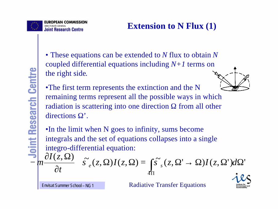
• These equations can be extended to N flux to obtain N coupled differential equations including N+1 terms on the right side.
•The first term represents the extinction and the N remaining terms represent all the possible ways in which radiation is scattering into one direction Ω from all other directions Ω’.
•In the limit when N goes to infinity, sums become integrals and the set of equations collapses into a single integro-differential equation:
Extension to N Flux (1)
')',()',(~),(),(~),(
4
ΩΩΩ→Ω=ΩΩ+∂
Ω∂− ∫
Π
dzIzzIzzI
se σστ
µ
Radiative Transfer Equations

29Envisat Summer School – NG 1
In the limit when N goes to infinity, sums become integrals and the set of equations collapses into a single integro-differential equation:
Extension to N Flux (2)
'd)',z(I)',z(~),z(I),z(~),z(I
4s ΩΩΩΩσΩΩσ
τΩ
µΠ∫ →=+
∂∂
−
I (z, Ω ) represents the intensity (W m-2sr-1) at point z in the exiting direction Ω,
σ (m-1) and σs (m-1sr-1) are the extinction and differential scattering coefficients, respectively, taken at the same point zalong the direction Ω.
Radiative Transfer Equations

30Envisat Summer School – NG 1
Vertical radiative coupling between geophysical media
Atmosphere
')',()',(~),()],,(~[4
ΩΩΩ→Ω=ΩΩΩ+∂∂
− ∫Π
dzIzzIz sOe σστ
µ
Radiative Transfer Equations
Vegetation
Soil
Upper limit (1)
RTE
Lower Limit (1)
Upper limit (2)
RTE
Lower Limit (2)
Upper limit (3)
RTE
Lower Limit (3)
ZA
ZV
ZS
Extinction coefficient Differential scattering coefficient
In each medium, the transfer of radiation may be represented by the following approximate equation:

31Envisat Summer School – NG 1
Vertical radiative coupling between geophysical media
Atmosphere
Radiative Transfer Equations
Vegetation
Soil
•Non oriented small scatterers
•Infinite number of scatterers
•Low density turbid medium
•Oriented finite-size scatterers
•Finite number of scatterers
•Dense discrete medium
•Oriented small-size scatterers
•Infinite number of clustered scatterers
•Compact semi-infinite medium

32Envisat Summer School – NG 1
Vertical radiative coupling between geophysical media
Atmosphere
Radiative Transfer Equations
Vegetation
Soil
Za
ZV
ZS
),( Ω↑a
zI)(),( 0 ota IzI Ω−Ω=Ω↓ δ
0),( =Ω∞↑ zI
The description of the interaction of a radiation field with a layered geophysical medium implies the solution of radiation transfer equations and the specification of appropriate boundary conditions
),(]||
exp[)(),(0
, Ω+−
Ω=Ω ↓↓↓bad
atatv zIzIzI
µτ
''',
'
2
||)(),,(1
),( ΩΩΩΩΠ
=Ω ↓
Π
↑ ∫ dzIzzI babavba µγ
''',
'
2
||)(),,(1
),( ΩΩΩΩΠ
=Ω ↓
Π
↑ ∫ dzIzzI bvbvsbv µγ

33Envisat Summer School – NG 1
Outline
• Scientific Problems with Space Remote Sensing
• Radiative Transfer Equations• Radiative Transfer Modeling for vegetation
canopy • RAMI • Conclusion

34Envisat Summer School – NG 1
Representation of vegetation canopy
‘Oriented’ scatterers elements in a finite volume à turbid medium
» Leaves are point-like scatterers
à discrete medium
» Leaves are finited-size scatterers
RT Vegetation Modeling

35Envisat Summer School – NG 1
Discrete canopy: 1D representation
Radiative Transfer Equations
H
Geometrical Parameters in 1D representation: Height of canopy, Size of a single leaf & Leaves orientation (leaf angle distribution)
Df

36Envisat Summer School – NG 1
N = # of layers
ai = leaf surface
ni = # leaves /m2
Vegetation Optical Depth
RT Vegetation Modeling
ii
N
1i
i
N
1i
anLAI ∑∑=
=
=
= λ
• Leaf Area Index (LAI) is a quantitative measure of the amount of live green leaf material present in the canopy per unit ground surface.
• It is defined as the total one-sided area of all leaves in the canopy within a defined region.

37Envisat Summer School – NG 1
N = # of layers
ai = leaf surface
ni = # leaves /m2
Vegetation Optical Depth
RT Vegetation Modeling
ii
N
1i
i
N
1i
anLAI ∑∑=
=
=
= λ
• Leaf Area Index (LAI) is a quantitative measure of the amount of live green leaf material present in the canopy per unit ground surface.
• It is defined as the total one-sided area of all leaves in the canopy within a defined region.

38Envisat Summer School – NG 1
H : Height of canopy [m]
∆ : Leaf Area Density [m2/m3]
Vegetation Optical Depth
RT Vegetation Modeling
∆.HLAI =
• Leaf Area Index (LAI) is a quantitative measure of the amount of live green leaf material present in the canopy per unit ground surface.
• It is defined as the total one-sided area of all leaves in the canopy within a defined region.

39Envisat Summer School – NG 1
Geometrical System
H
z
Ωo
North
Ω
φοφ
θ
θο

40Envisat Summer School – NG 1
Extinction coefficient
RT Vegetation Modeling
),,(~Oe z ΩΩσ
We assume that the canopy consists of plane leaves with a leaf area density λ(z) defined to be the total one-sided leaf area per unit volume at depth z.The probability that a leaf has a normal directed away from the top surface, in a unit solid angle about is given by the leaf-normal distribution function which is normalized as
lll ϕ,?O
lO
),( ll Ωzg
1),(21
2
1
0
=Ω∫ ∫π
µφπ llll zgdd
')',()',(~),()],,(~[4
ΩΩΩ→Ω=ΩΩΩ+∂∂
− ∫Π
dzIzzIz sOe σστ
µ
plate model
OL

41Envisat Summer School – NG 1
Extinction coefficient
RT Vegetation Modeling
We now consider photons at a depth z travelling in direction Ω.The extinction coefficient is then the probability, per unit path length, that the photon hits a leaf, i.e., the probability that a photon while traveling a distance ds along Ω is intercepted by a leaf divided by the distance ds.
Where the geometry factor G is the fraction of the total leaf area (per unit volume of the canopy) that is perpendicular to Ω
( ) ( ) )(,, zzGze lλσ Ω=Ω
lll ΩΩ•ΩΩ=Ω ∫ dgzG ||)(21
),(2ππ
Ref: Ross (1981)

42Envisat Summer School – NG 1
Ref: Ross (1981)
Leaf OrientationsVegetation foliage features characteristic leaf-normal distributions, g(OL) with preferred:
• azimuthal orientations, g(f L)
• zenithal orientations, g(?L):
Ø erectophile (grass) (90o)
Ø planophile (water cress) (0o)
Ø plagiophile (45o)
Ø extremophile (0o and 90o)
Ø uniform/spherical (all)
• time varying orientations:Ø heliotropism (sunflower)
Ø para-heliotropism
RT Vegetation Modeling

43Envisat Summer School – NG 1
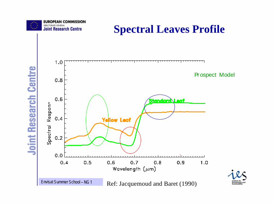
• Directionality of leaf scattering depends on the leaf surface roughness, and the percentage of diffusely scattered photons from leaf interior.
• Leaf reflection and transmissiondepend primarily on wavelength, plant species, growth condition, age and position in canopy.
OL
plate model
O
O
Ø Plate models often assume Bi-Lambertian scattering properties: - radiation is scattered according to cosine law: | OL · O | - magnitude depends on leaf reflection and transmission values
RT Vegetation Modeling
Scattering properties of leaves
Ref: Ross (1981)
• Once the radiation is intercepted by the vegetation elements, it is scattered in directions determined by the leaf orientationsand the leaf phase function

44Envisat Summer School – NG 1
Leaf scattering properties
• Leaf scattering function for classical plate scattering model
Where rl and tl are the fraction of intercepted energy which are reflected (transmitted) following a simple cosine distribution law around the normal to the leaves.
πΩΩΩΩΩ
πΩΩΩΩΩ
/||t),(f
/||r),(f'
'
lll
lll
•=→
•=→
0))((if
0))((if'
'
>••
<••
ll
ll
ΩΩΩΩ
ΩΩΩΩ
45Envisat Summer School – NG 1
Spectral Leaves Profile
Prospect Model
Ref: Jacquemoud and Baret (1990)

46Envisat Summer School – NG 1
Canopy scattering phase function
• Leaf properties are assumed to be the same throughout the canopy, we have
g (ΩL) is the probability function for the leaf normal distribution ΩL
f is the leaf phase function (when integrated over all exit photons directions, yields single scattering albedo ω).
lll ΩΩΩΩΩΩΩπ
ΩΩΓπ
ΩΩΓπ
ΩΩΓπ
π
d),(f||)(g21
)(1
)(1
),z(1
''
2
'
''k
→•≡→
→≡→
∫
Ref: Shultis & Myneni (1988) and Knyazihin et. al. (1992)

47Envisat Summer School – NG 1
Specific Effects
•The presence of finite size scatterers implies that the radiation interception process by the leaves will not follow a continuous scheme, and in particular that radiation will be allowed to travel unimpeded within the free space between the scatterers.
•Since extinction occurs only at discrete locations, some of the radiation emerging from an arbitrary source, located inside or outside the canopy, any occasionally travel without any interaction in this canopy, depending on the shape and size of free space between these leaves.
Radiative Transfer EquationsRef: Verstraete et. al. (1990) Ref: Gobron et al. (1997)

48Envisat Summer School – NG 1
Hot-spot Effects
Radiative Transfer Equations
•When the radiation is scattered back in the direction from which it originates, the probability of further interaction with the canopy is lower than in other scattering directions.
•In case of RS measurements outside the canopy, this give rise to a relative increase in the value in the backscattering direction which is knows as the hot-spot phenomenon.
Ref: Verstraete et. al. (1990) Ref: Gobron et al. (1997)

49Envisat Summer School – NG 1
Hot-spot EffectsExtinction coefficient is modified adding hot-spot scale factor: se(z, O, O0) = ?(z) · G(O)· O(z, O, O0)
observation zenith angle [degree]-90 -45 0 45 90
Bi-d
irect
iona
l Ref
lect
ance
Fac
tor
(?=
Red
)
0.08
0.06
0.04
0.02
0.00
1-D’
1-D
Radiative Transfer Equations
Turbid canopy representation: 1-D
O = O0
illuminated leaf
O0O
Ref: Verstraete et. al. (1990) Ref: Gobron et al. (1997)

50Envisat Summer School – NG 1
Separation of Scattering Order
• Uncollided intensity
),,z(),,z(),,z(),,z( 00000000 M10 ΩΩρΩΩρΩΩρΩΩρ ++=
Ref: Gobron et al. (1997)

51Envisat Summer School – NG 1
Separation of Scattering Order
• Uncollided intensity• Single Collided intensity
),,z(),,z(),,z(),,z( 00000000 M10 ΩΩρΩΩρΩΩρΩΩρ ++=
Ref: Gobron et al. (1997)

52Envisat Summer School – NG 1
Separation of Scattering Order
• Uncollided intensity• Single Collided intensity• Multiple scattering intensity
),,z(),,z(),,z(),,z( 00000000 M10 ΩΩρΩΩρΩΩρΩΩρ ++=
Ref: Gobron et al. (1997)

53Envisat Summer School – NG 1
Uncollided intensity (1)
k
0
0s0k
0
||)(G
1I),z(I
−=↓ µ
ΩλΩ
Downward uncollided intensity at level zk
Where is the incoming
collimated beam at the top of canopy
)(),z(II 0000
s ΩΩδΩ −=
Probability that a light ray within this beam is transmitted
downward in the same direction through the first k layers
Ref: Gobron et al. (1997)

54Envisat Summer School – NG 1
Uncollided intensity (2)
K
0
0s00s0
0
||)(G
1I||),,H(1
),,H(I
−=↑ µ
ΩλµΩΩγ
πΩΩ
The radiation scattered by the soil, which provides the lower radiative boundary condition of the canopy system, for uncollided radiation is given by:
Where denotes the bidirectional reflectance factor of the soil at the bottom of canopy.
),,H( 0s ΩΩγ
∏+
=
−
−=↑
1k
Kj
'K
K
0
0s00s0k
0 )(G1
||)(G
1I||),,H(1
),,z(IµΩ
λµΩ
λµΩΩγπ
ΩΩ
Ref: Gobron et al. (1997)
55Envisat Summer School – NG 1
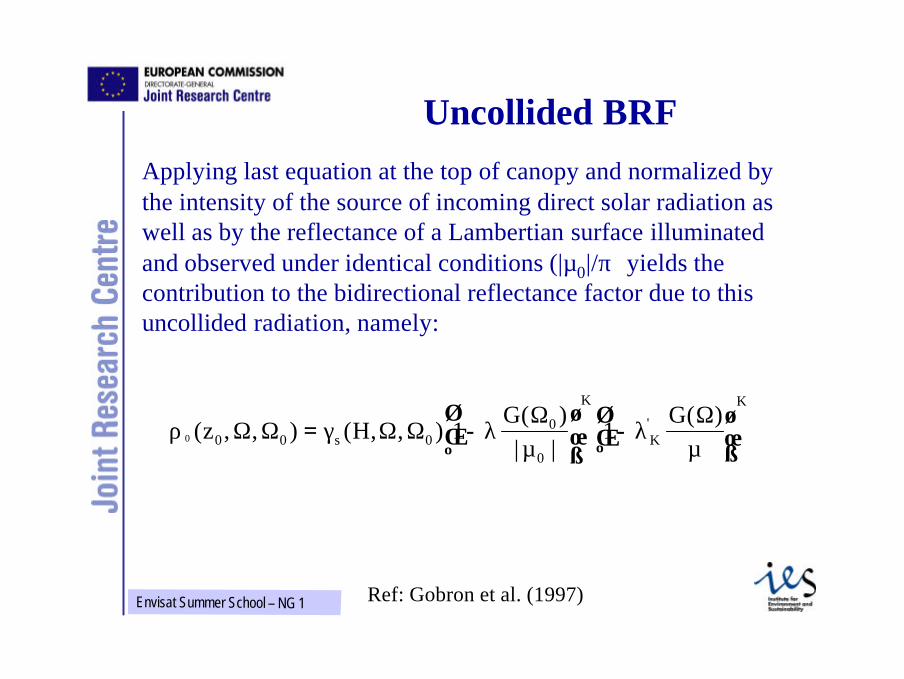
Applying last equation at the top of canopy and normalized by the intensity of the source of incoming direct solar radiation as well as by the reflectance of a Lambertian surface illuminated and observed under identical conditions (|µ0|/π) yields the contribution to the bidirectional reflectance factor due to thisuncollided radiation, namely:
Uncollided BRF
K
'K
K
0
00s00
)(G1
||)(G
1),,H(),,z(0
−
−=
µΩ
λµΩ
λΩΩγΩΩρ
Ref: Gobron et al. (1997)
56Envisat Summer School – NG 1
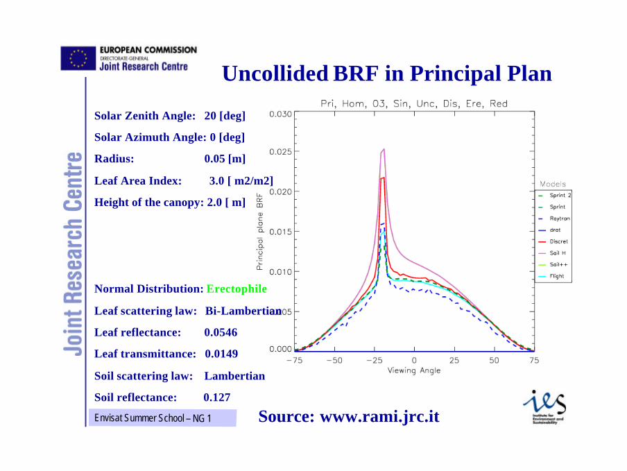
Uncollided BRF in Principal Plan
Source: www.rami.jrc.it
Solar Zenith Angle: 20 [deg]
Solar Azimuth Angle: 0 [deg]
Radius: 0.05 [m]
Leaf Area Index: 3.0 [ m2/m2]
Height of the canopy: 2.0 [ m]
Normal Distribution: Erectophile
Leaf scattering law: Bi-Lambertian
Leaf reflectance: 0.0546
Leaf transmittance: 0.0149
Soil scattering law: Lambertian
Soil reflectance: 0.127

57Envisat Summer School – NG 1
Uncollided BRF in Principal Plan
Source: www.rami.jrc.it
Solar Zenith Angle: 20 [deg]
Solar Azimuth Angle: 0 [deg]
Radius: 0.05 [m]
Leaf Area Index: 3.0 [ m2/m2]
Height of the canopy: 2.0 [ m]
Normal Distribution: Erectophile
Leaf scattering law: Bi-Lambertian
Leaf reflectance 0.4957
Leaf transmittance 0.4409
Soil scattering law Lambertian
Soil reflectance 0.159

58Envisat Summer School – NG 1
Uncollided BRF in Cross Plan
Source: www.rami.jrc.it
Solar Zenith Angle: 20 [deg]
Solar Azimuth Angle: 0 [deg]
Radius: 0.05 [m]
Leaf Area Index: 3.0 [ m2/m2]
Height of the canopy: 2.0 [ m]
Normal Distribution: Erectophile
Leaf scattering law: Bi-Lambertian
Leaf reflectance: 0.0546
Leaf transmittance: 0.0149
Soil scattering law: Lambertian
Soil reflectance: 0.127

59Envisat Summer School – NG 1
Uncollided BRF in Cross Plan
Source: www.rami.jrc.it
Solar Zenith Angle: 20 [deg]
Solar Azimuth Angle: 0 [deg]
Radius: 0.05 [m]
Leaf Area Index: 3.0 [ m2/m2]
Height of the canopy: 2.0 [ m]
Normal Distribution: Erectophile
Leaf scattering law: Bi-Lambertian
Leaf reflectance 0.4957
Leaf transmittance 0.4409
Soil scattering law Lambertian
Soil reflectance 0.159

60Envisat Summer School – NG 1
First collided Intensity (1)
The first collided intensity in downward direction Ω corresponds to the radiation scattered only once by leaves, but which has not interacted with the soil.
•Downward source coming from the direct intensity, attenuated through the first k layers, and scattered by the leaves according to their optical properties in layer k:
•Downward intensity
k
0
0s00k
0
||)(G
1I)(1
),,z(Q
−→=↓ µ
ΩλΩΩΓ
πΩΩ
ikk
1i0i
00k
1
||)(G
1),,z(Q1
),,z(I−
=↓↓
−= ∑ µ
ΩλλΩΩ
µΩΩ
Ref: Gobron et al. (1997)

61Envisat Summer School – NG 1
First collided Intensity (2)
The first collided intensity in downward direction Ω corresponds to the radiation scattered only once by leaves, but which has not interacted with the soil.
•Downward intensity
•Upward intensity
ikk
1i0i
00k
1
||)(G
1),,z(Q1
),,z(I−
=↓↓
−= ∑ µ
ΩλλΩΩ
µΩΩ
−×= ∏∑
+
=
+
=↓↑
1k
ij
'i
1k
Ki0i
00k
1
||)(G
1),,z(Q1
),,z(IµΩ
λλΩΩµ
ΩΩ
Ref: Gobron et al. (1997)

62Envisat Summer School – NG 1
Single collided BRF
The contribution to the bidirectional reflectance factor due to the first collided intensity is obtained after normalizing the upward intensity by the incoming directional source of radiation at the top of canopy:
),,( 001 ΩΩ↑ zI
( ) i
K
i
Ki
GGz
Ω−
Ω−
Ω→ΩΓ=ΩΩ ∑
= µλ
µλλ
µµρ
)(1
||)(
1||
),,( '
0
01
0
0001
Ref: Gobron et al. (1997)

63Envisat Summer School – NG 1
Single Collided BRF in Principal Plan
Source: www.rami.jrc.it
Solar Zenith Angle: 20 [deg]
Solar Azimuth Angle: 0 [deg]
Radius: 0.05 [m]
Leaf Area Index: 3.0 [ m2/m2]
Height of the canopy: 2.0 [ m]
Normal Distribution: Erectophile
Leaf scattering law: Bi-Lambertian
Leaf reflectance: 0.0546
Leaf transmittance: 0.0149
Soil scattering law: Lambertian
Soil reflectance: 0.127

64Envisat Summer School – NG 1
Single Collided BRF in Cross Plan
Source: www.rami.jrc.it
Solar Zenith Angle: 20 [deg]
Solar Azimuth Angle: 0 [deg]
Radius: 0.05 [m]
Leaf Area Index: 3.0 [ m2/m2]
Height of the canopy: 2.0 [ m]
Normal Distribution: Erectophile
Leaf scattering law: Bi-Lambertian
Leaf reflectance: 0.0546
Leaf transmittance: 0.0149
Soil scattering law: Lambertian
Soil reflectance: 0.127

65Envisat Summer School – NG 1
Single collided BRF in Principal Plan
Source: www.rami.jrc.it
Solar Zenith Angle: 20 [deg]
Solar Azimuth Angle: 0 [deg]
Radius: 0.05 [m]
Leaf Area Index: 3.0 [ m2/m2]
Height of the canopy: 2.0 [ m]
Normal Distribution: Erectophile
Leaf scattering law: Bi-Lambertian
Leaf reflectance 0.4957
Leaf transmittance 0.4409
Soil scattering law Lambertian
Soil reflectance 0.159
66Envisat Summer School – NG 1
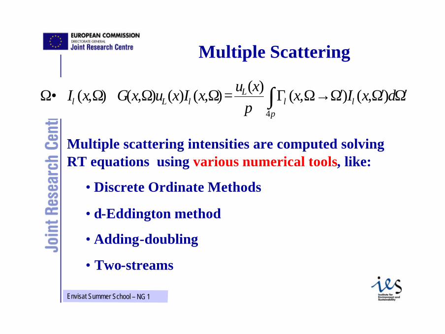
Multiple Scattering
Multiple scattering intensities are computed solving RT equations using various numerical tools, like:
• Discrete Ordinate Methods
• δ-Eddington method
• Adding-doubling
• Two-streams
Ω•∇Iλ(x,Ω)+G(x,Ω)uL(x)Iλ(x,Ω)= uL(x)π
Γλ(x,Ω→ ′ Ω )Iλ(x, ′ Ω )d ′ Ω 4π∫

67Envisat Summer School – NG 1
Multiple Scattering

68Envisat Summer School – NG 1
3-Dimensional problem
where the plan-parallel concept may be inappropriate

69Envisat Summer School – NG 1
Coniferous trees onto a Gaussian shaped topography
Structurally heterogeneous trees at various res.
270 x 270 x 15 m
Clumping of leaves into floating spheres
100 x 100 x 30 m
500 x 500 x 114 m
Examples of Scenes
70Envisat Summer School – NG 1
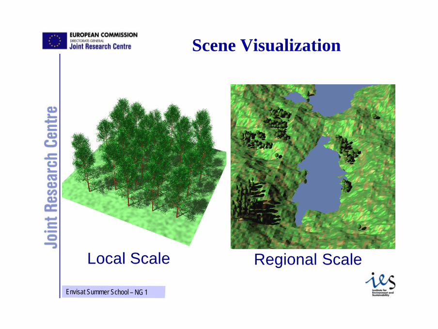
Local Scale Regional Scale
Scene Visualization

71Envisat Summer School – NG 1
3-Dimensional problem
where the plan-parallel concept may be inappropriate:
•Document the errors due to an oversimplification of the full 3-D situation, i.e. deviations from the 1D case.
•Explore new ways and techniques for representing, at limited costs, the 3D nature of the medium which basically require almost an infinity of parameters!
•Address the application issues for geophysical modeling, e.g. the definition of new “equivalent variables”, and satellite data interpretation, e.g. the non-uniqueness of the inverse problem.

72Envisat Summer School – NG 1
3-D Radiative Transfer Equations
3-D Models
•Ray tracing models
•Geometrical models
•Hybrid models
Ω•∇Iλ(x,Ω)+G(x,Ω)uL(x)Iλ(x,Ω)= uL(x)π
Γλ(x,Ω→ ′ Ω )Iλ(x, ′ Ω )d ′ Ω 4π∫

73Envisat Summer School – NG 1
Outline
• Scientific Problems with Space Remote Sensing
• Radiative Transfer Equations• Radiative Transfer Modeling for vegetation
canopy • RAMI • Conclusion

74Envisat Summer School – NG 1

75Envisat Summer School – NG 1

76Envisat Summer School – NG 1
Model Benchmarking

77Envisat Summer School – NG 1
Outline
• Scientific Problems with Space Remote Sensing
• Radiative Transfer Equations• Radiative Transfer Modeling for vegetation
canopy • 3D models• RAMI • Conclusion

78Envisat Summer School – NG 1
Conclusion• RT modeling in vegetation: two-stream RT
equations, 1D turbid canopy, 1D’ discrete model & 3D heterogeneous canopy model
• All models require spectral scattering and absorption canopies properties
… and assumptions • RAMI exercise for direct mode comparison and
validation
• The fun with RT models with space remote sensing data comes with the inversion mode … tomorrow !