Radia%ve-­‐transfer  Modeling  of  Type  II  Supernova  

Luc  Dessart Observatoire de la Cote d’Azur, Nice, France  

In  collabora%on  with  John  Hillier  (Univ.  PiEsburgh)  

Roni  Waldman  &  Eli  Livne  (Racah  Inst.,  Jerusalem)  Stan  Woosley  (UC  Santa  Cruz)    

Ph.D  student:  Sergey  Lisakov  (Nice)  

1.  Aims  

2.  Observa%onal  background  

3.  Theore%cal  background  

4.  Numerical  approaches  for  Type  II  SN  modeling  (pre-­‐SN,  explosion,  SN  rad.)  

5.  Radia%ve  transfer  simula%ons  with  CMFGEN  and  other  codes  

6.  Results  from  photospheric  &  nebular  phases  

7.  Constraints  on  ejecta  proper%es  and  progenitors  

8.  SNe  II-­‐P  as  metallicity  probes  

Layout  

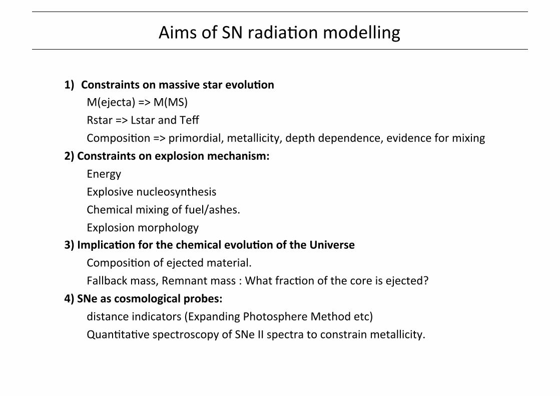
Aims  of  SN  radia%on  modelling  

1)  Constraints  on  massive  star  evolu1on                  M(ejecta)  =>  M(MS)                  Rstar  =>  Lstar  and  Teff                  Composi%on  =>  primordial,  metallicity,  depth  dependence,  evidence  for  mixing    2)  Constraints  on  explosion  mechanism:                  Energy                  Explosive  nucleosynthesis                  Chemical  mixing  of  fuel/ashes.                  Explosion  morphology  3)  Implica1on  for  the  chemical  evolu1on  of  the  Universe                  Composi%on  of  ejected  material.                  Fallback  mass,  Remnant  mass  :  What  frac%on  of  the  core  is  ejected?  4)  SNe  as  cosmological  probes:                  distance  indicators  (Expanding  Photosphere  Method  etc)                  Quan%ta%ve  spectroscopy  of  SNe  II  spectra  to  constrain  metallicity.      

Observa%onal  proper%es  of  core-­‐collapse  SNe  

SN  Classifica1on:    Type  II:  HI  lines.                      IIn:    narrow  lines    Type  I  :  No  HI  line  =>  Ib:  He  I  lines                                                                      =>  Ic:    No  He  I  line                                                                    =>  Ic-­‐BL:  Ic  broad  lines  Hybrid  type  IIb:  HI  &  HeI  lines                

=>  Reflects  composi1on  differences  

Observa%onal  proper%es  of  core-­‐collapse  SNe  

Light-­‐curve  types:    Plateau:  Type  II-­‐P  Bell-­‐shape:    Type  I  Hybrid:  e.g.  SN  1987A  (II-­‐peculiar)  

0 20 40 60 80 100 120 140 160 180Days since explosion

�19

�18

�17

�16

�15

�14

�13

MV

[mag

]

Ic-BLIcIbIIbIIPII-pec

=>  Reflects  varia1ons  in  R★,  M★,  Eexpl,  and    M(56Ni)    

Type  II  SN  light  curve  diversity  

•  Range  of  LC  slopes  from  plateau  to  linear:  II-­‐P  versus  II-­‐L  •  Range  of  peak/plateau  brightness  (-­‐14  to  -­‐18mag)  and  late-­‐%me  brightness  •  Range  of  bright-­‐phase  dura%on  (50  to  100+  days)  

The Astrophysical Journal, 786:67 (35pp), 2014 May 1 Anderson et al.

Table 2(Continued)

SN Classification No. of Spectra Epochs of Spectra CommentsReference

2009au Stritzinger et al. (2009) 7 +24, +80 Originally classified as type IIn, however spectrum showsclear Hα absorption, and light-curve is of “plateau” morphology.

Narrow lines are most likely related to underlying starformation region (as indicated by 2d spectrum)

2009bu Morrell & Stritzinger (2009) 6 +12, +672009bz Challis & Berlind (2009a) 4 +9, +37 Spectra indicate hydrogen-rich type II event

Notes. Spectroscopic information used for classification of the current sample as hydrogen-rich type II events. In the first column the SN name is listed,followed by the classification circular references. We then indicate the number of spectra which were obtained, and that are used for: NaD EW measurements,explosion time estimations, and confirmation of type classifications in Column 3, followed by the epoch of the first and last spectrum in Column 4. In Column 5comments are listed in cases where: (a) the circular classification information is sparse, (b) spectra have been previously analyzed, (c) distinct spectroscopyhas been published in the literature, and (d) in cases where we have changed the classification from that quoted in the circulars.

Figure 1. Example of the light-curve parameters measured for each SN.Observed magnitudes at peak, Mmax, end of “plateau,” Mend, and beginningof linear decline, Mtail are shown in blue, as applied to the example dummydata points (magenta). The positions of the three measured slopes: s1, s2, ands3 are shown in green. The time durations: “plateau” length, Pd, and opticallythick phase duration, OPTd are indicated in black. Four time epochs are labeled:t0, the explosion epoch; ttran, the transition from s1 to s2; tend, the end of theoptically thick phase; and tPT, the mid point of the transition from “plateau” toradioactive tail.(A color version of this figure is available in the online journal.)

Section 3.1) and tPT: the mid-point of the transition betweenplateau and linear decline epochs obtained through fitting SN IIlight-curves with the sum of three functions: a Gaussian whichfits to the early time peak/decline; a Fermi Dirac function whichprovides a description of the transition between the plateau andradioactive phases; and a straight line which accounts for theslope due to the radioactive decay (see Olivares E. et al. 2010 forfurther description). It is important to note here, while the fittingprocess of tPT appears to give good objective estimations of thetime epoch of transition between plateau and later radioactivephases, its fitting of precise parameters such as decline rates,together with magnitudes and epochs of maximum light is lesssatisfactory. Therefore, we employ this fitting procedure solelyfor the measurement of the epoch tPT (from which other timeepochs are defined). In the future, it will be important to buildon current template fitting techniques of SNe II light-curves, in

order to measure all parameters in a fully automated way. Forthe current study, we continue as outlined below.

With the above epochs in hand, the measured parameters are:

1. Mmax: defined as the initial peak in the V-band light-curve.Often this is not observed, either due to insufficient earlytime data or poorly sampled photometry. In these cases wetake the first photometric point to be Mmax. When a truepeak is observed, it is measured by fitting a low order (fourto five) polynomial to the photometry in close proximity tothe brightest photometric point (generally ±5 days).

2. Mend: defined as the absolute V-band magnitude measured30 days before tPT. If tPT cannot be defined, and thephotometry shows a single declining slope, then Mend ismeasured to be the last point of the light-curve. If the end ofthe plateau can be defined (without a measured tPT) then wemeasure the epoch and corresponding magnitude manually.

3. Mtail: defined as the absolute V-band magnitude measured30 days after tPT. If tPT cannot be estimated, but it is clearlyobserved that the SN has fallen onto the radioactive decline,then Mtail is measured taking the magnitude at the nearestpoint after transition.

4. s1: defined as the decline rate in magnitudes per 100 days ofthe initial, steeper slope of the light-curve. This slope is notalways observed either because of a lack of early time data,or because of insufficiently sampled light-curves However,in some instances a lack of detection may simply imply alack of any true peak in the light-curve, together with anintrinsic lack of an early decline phase.

5. s2: defined as the decline rate (V-band magnitudes per100 days) of the second, shallower slope in the light curve.This slope is that referred to in the literature as the “plateau.”We note here, there are many SNe within our sample whichhave light-curves which decline at a rate which is ill-described by the term “plateau.” However, in the majoritySNe II in our sample (with sufficiently sampled photometry)there is suggestive evidence for a “break” in the light-curvebefore a transition to the radioactive tail (i.e., an end to a“plateau” or optically thick phase). Therefore, hereafter weuse the term “plateau” in quotation marks to refer to thisphase of nearly constant decline rate (yet not necessarily aphase of constant magnitude) for all SNe.

6. s3: defined as the linear decline rate (V-band magnitudesper 100 days) of the slope reached by each transientafter its transition from the previous “plateau” phase.This is commonly referred to in the literature as theradioactive tail.

8

Anderson+14  

The Astrophysical Journal, 786:67 (35pp), 2014 May 1 Anderson et al.

Figure 2. SNe II absolute V-band light-curves of the 60 events with explosionepochs and AV corrections. Light-curves are displayed as Legendre polynomialfits to the data, and are presented by black lines. For reference we also show incolors the fits to our data for four SNe II: 1986L, 1999em, 2008bk, and 1999br.(A color version of this figure is available in the online journal.)

with an accompanying lower limit to the probability of findingsuch a correlation strength by chance.22 Where correlations arepresented with parameter pairs (N) higher than 20, binned datapoints are also displayed, with error bars taken as the standarddeviation of values within each bin.

4.1. SN II Parameter Distributions

In Figure 3 histograms of the three absolute V-band magni-tude distributions: Mmax, Mend and Mtail are presented. Thesedistributions evolve from being brighter at maximum, to lowerluminosities at the end of the plateau, and further lower valueson the tail. Our SN II sample is characterized, after correction forextinction, by the following mean values: Mmax = −16.74 mag(σ = 1.01, 68 SNe); Mend = −16.03 mag (σ = 0.81, 69 SNe);Mtail = −13.68 mag (σ = 0.83, 30 SNe).

The SN II family spans a large range of ∼4.5 mag at peak,ranging from −18.29 mag (SN 1993K) through −13.77 mag(SN 1999br). At the end of their “plateau” phases the sampleranges from −17.61 to −13.56 mag. SN II maximum light ab-solute magnitude distributions have previously been presentedby Tammann & Schroeder (1990) and Richardson et al. (2002).Both of these were B-band distributions. Tammann & Schroederpresented a distribution for 23 SNe II of all types of MB =−17.2 mag (σ = 1.2), while Richardson et al. found MB =−17.0 mag (σ = 1.1) for 29 type IIP SNe and MB = −18.0 mag(σ = 0.9) for 19 type IIL events. Given that our distributionsare derived from the V band, a direct comparison to these worksis not possible without knowing the intrinsic colors of each SN

22 Calculated using the on-line statistics tool found at:http://www.danielsoper.com/statcalc3/default.aspx (Cohen et al. 2003).

Figure 3. Histograms of the three measured absolute magnitudes of SNe II.Top: peak absolute magnitudes; Mmax. Middle: absolute magnitudes at the endof the plateau; Mend. Bottom: absolute magnitudes at the start of the radioactivetail; Mtail. In each panel the number of SNe is listed, together with the meanabsolute V-band magnitude and the standard deviation on that mean.(A color version of this figure is available in the online journal.)

within both samples. However, our derived Mmax distribution isreasonably consistent with those previously published (althoughslightly lower), with very similar standard deviations.

At all epochs our sample shows a continuum of absolutemagnitudes, and the Mmax distribution shows a low-luminositytail as seen by previous authors (e.g., Pastorello et al. 2004; Liet al. 2011). All three epoch magnitudes correlate strongly witheach other: when a SN II is bright at maximum light it is alsobright at the end of the plateau and on the radioactive tail.

Figure 4 presents histograms of the distributions of the threeV-band decline rates, s1, s2 and s3, together with their meansand standard deviations. SNe decline from maximum (s1) atan average rate of 2.65 mag per 100 days, before decliningmore slowly on the “plateau” (s2) at a rate of 1.27 mag per100 days. Finally, once a SN completes its transition to theradioactive tail (s3) it declines with a mean value of 1.47 magper 100 days. This last decline rate is higher than that expectedif one assumes full trapping of gamma-ray photons from thedecay of 56Co (0.98 mag per 100 days, Woosley et al. 1989).This gives interesting constraints on the mass extent and densityof SNe ejecta, as will be discussed below. We observe morevariation in decline rates at earlier times (s1) than during the“plateau” phase (s2).

As with the absolute magnitude distributions discussed above,the V-band decline rates appear to show a continuum in theirdistributions. The possible exceptions are those SNe decliningextremely quickly through s1: the fastest decliner SN 2006Ywith an unprecedented rate of 8.15 mag per 100 days. In thecase of s2 the fastest decliner is SN 2002ew with a decline rateof 3.58 mag per 100 days, while SN 2006bc shows a rise duringthis phase, at a rate of −0.58 mag per 100 days. The s2 declinerate distribution has a tail out to higher values, while a sharp

12

=>  Reflects  varia1ons  in  R★,  M(H-­‐env),  Eexpl  

 Type  II  SN  Spectral  Evolu%on

Spectral evolution reflects evolution of τ, composition, ionization, excitation, T, Vphot(m)

Nebular  phase:  τcont  <1  

Photospheric  phase:  τcont  >1  

P-­‐Cygni  profiles.  Early:  blue  cont.,  weak  blanke%ng  Late:  Recombina%on,  strong  blanke%ng  Probes  H-­‐rich  envelope  

Pseudo-­‐con%nuum  from  lines  (FeI,  FeII)  τline  >1  even  if  τcont  <1  P-­‐Cygni  profiles  for  thick  lines  Boxy  profiles  for  forbidden  (thin)  lines  Probes  inner  &  outer  ejecta    

EPM DISTANCE TO SN 1999em 45

2002 PASP, 114:35–64

Fig. 6.—Optical flux spectra of SN 1999em spanning the first 96 days afterdiscovery. In this and all figures a recession velocity of 800 km s!1 has beenremoved from the observed spectrum (§ 2.2.3). Note that the continuum shapeof the spectra on days 5 and 6 has been manually adjusted redward of 5800 Abecause of irregularities introduced by the spectrograph.

Fig. 7.—Optical and near-infrared spectral development of SN 1999em dur-ing its first 517 days after discovery (1999 October 29). Six plateau-phasespectra shown in Fig. 6 are reproduced here as well, but with their full spectralrange displayed.

light loss (Filippenko 1982). In addition, the shape of all spectraobtained with the Lick 1 m reflector is suspect, especially atwavelengths greater than 5800 A, since successive observationsfrom the same night occasionally showed significant varia-tions.19 Multiple extractions of the data using apertures of var-ying width and different background regions failed to remedythe problem, and its cause remains unknown. Fortunately, thiscalibration uncertainty has minimal scientific impact here sinceit is the wavelengths of absorption features, not absolute fluxes,that are of primary interest. In any case, the effect was evidenton only a few nights, and quantities derived using spectra ob-tained on these nights are in good agreement with those derivedfrom spectra taken at other telescopes.The spectral evolution of SN 1999em during the first

517 days of its development is shown in Figures 6 and 7. Theearly spectra are characterized by a nearly featureless contin-

19 Normalizing the spectrum at the blue end, the flux level of the red endvaried by as much as !30% on the worst nights.

uum with broad hydrogen Balmer and He i l5876 P Cygnilines. As early as day 7, a hint of Fe ii l5169 absorption isvisible, and it becomes quite strong by day 11 along withFe ii l5018. During the next 90 days the strength of numerousmetal lines continues to increase (see Fig. 1). After the plateauends, the spectrum becomes more emission dominated andmarked by the presence of such forbidden lines as [Ca ii]ll7291, 7324 and [O i] ll6300, 6364.As discussed in § 1, one area of uncertainty in the application

of EPM is estimating the photospheric velocity. To test theconsistency of velocities measured from different lines, we shallderive velocities from as many features as possible in the opticalspectrum of SN 1999em during the photospheric phase. Ourgoal is to identify several unblended, weak features and com-pare the velocity derived using them with that obtained fromthe Fe ii ll4924, 5018, 5169 lines, which have often beenused in previous EPM studies.We first identified 36 distinct absorption features in the op-

tical photospheric spectrum of SN 1999em, focusing mainlyon the region between 4000 and 7000 A since that range was

Leonard  et  al.  (2002)  

Basics  of  core-­‐collapse  SNe  

•  Massive-­‐star  graveyard  (M≥8M¤).    •  Collapse  of    Mch  Fe  core  to  a  neutron  star  releases  1053erg.    •  Explosion  powered  by  neutrinos  ;  rota%on  boost  ?  Other  processes?    •  1  min  to  1  day:  shock  propagates  and  breaks  out  (1st  EM  signature).    •  Ejecta  proper%es:  Ekin~1051erg  

                                                                             Mejecta~  few  M�                                                                                Vexp~3000km/s                                                                                M(56Ni)  ~  0.1M�    

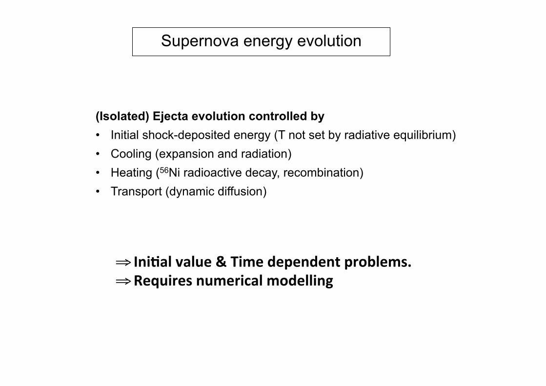
Supernova energy evolution

⇒ Ini1al  value  &  Time  dependent  problems.  ⇒ Requires  numerical  modelling  

(Isolated) Ejecta evolution controlled by •  Initial shock-deposited energy (T not set by radiative equilibrium) •  Cooling (expansion and radiation) •  Heating (56Ni radioactive decay, recombination) •  Transport (dynamic diffusion)

Numerical  modeling  of  Type  II  SN  radia%on:  Approaches  

•  Simula1on  of  progenitor:  polytrope,  model  evolved  from  MS  to  collapse.  

•  Simula1on  of  Explosion:  Radia%on  Hydrodynamics  using  thermal  bomb  /  piston.  

Grey  or  mul%-­‐group  approach.  Nuclear  network  (nucleosynthesis).  

•  Simula1on  of  Ejecta/radia1on:  

                     Grey/mul1-­‐group  RHD  =>  Light  curve,  colors,  Vphot  (cheap)  

                     RHD  +  non-­‐LTE  Radia1ve  Transfer  (cruising  phase)  

                                                                                                       Time-­‐dependent  RT  (costly)  =>  LC/colors,  spectra  

                                                                                             Steady-­‐state  RT  (cheap)                =>  spectra  

Non-LTE Time-Dependent Radiative Transfer Modeling with cmfgen (Hillier & Miller 1998; Dessart & Hillier 2005ab,2008, 2010; Hillier & Dessart 2012)

∑≠

−==ij

ijijijii RnRn

DtnrD

rDtnD )()(1)/( 3

3ρ

ρRate Equation:

∫∞

−=− 0 )(4 νχπρ

ρρ ννν dSJ

DtDP

DtDe

Energy Equation:

where

nmEn

nmnnkT

e

H

ii

H

e

µµ∑+

+=

=

)(

masst energy/uni internl

23

νννν χην

ν JJrcV

rHr

rDtJrD

cr−=

∂∂

−∂

∂+

)(1)(1 2

2

3

3

νννννν χν

ν HHrcV

rJK

rKr

rDtHrD

cr−=

∂∂

−−

+∂

∂+

)(1)(1 2

2

3

3

RTE 0th moment:

RTE 1st moment:

Rad

iatio

n G

as

Cou

plin

g

+ Dedecay/Dt

(Excitation + Ionization)

& charge conservation

Radia%ve  transfer  with  cmfgen:  code  characteris%cs  

•  Assumes  Spherical  Symmetry  and  homologous  expansion  

•  Time-­‐dependent  transport:  moments  of  RTE  with  all  important  terms  in  v/c,  ∂/∂t,  ∂/∂ν,(∂/∂µ),  ∂/∂r    

•  Sta%s%cal  Equilibrium  Equa%ons  =>  non-­‐LTE  solver  (concept  of  super-­‐levels)  

•  De/Dt  &  Dn/Dt  =>  Time-­‐dependent  ionisa%on  

•  Account  for  opacity  ν-­‐by-­‐ν.  Line  blanke%ng.    

•  Non-­‐local  energy  deposi%on  (γ-­‐ray  Monte  Carlo  code)    

•  Non-­‐thermal  processes  (solu%on  to  Spencer-­‐Fano  equa%on  =>  non-­‐thermal  rates)  

•  Full-­‐ejecta  simula%on  at  all  %mes    (no  “ar%ficial”  BC,  Xi  stra%fica%on)    

=>  Code  naturally  evolves  from  thick  to  thin  condi%ons  

•  Flux:  computed  at  ~105  ν  from  X-­‐ray  range  to  far-­‐IR.    

•  Time  evolu%on:  0.5-­‐1  d  to  few  100d  aqer  explosion  (Δt  =  0.1t)  

Illustrations with non-LTE Steady-state approach

•  Neglect D/Dt terms •  Model the photospheric regions only (like for stars) •  Impose Flux at inner boundary + Radiative equilibrium •  Advantage : Flexibility.

•  Application to SNe II-P (e.g., SN2005cs) •  Exploration on spectral dependencies

Non-LTE Steady State Approach Application: Modeling of Young Type II SNe

The case of the Type II-P SN 2005cs in NGC 5194 (Dessart et al. 2008)

SN II-P spectra: Dependencies

•  Z modulates metal-line blanketing •  ρ(v) modulates τline and τcont •  H/He in SN II-P: influences UV flux

but HI lines poorly sensitive

Degenerate effect of E(B-V) and T. Use lines

Time dependent approach

•  Include D/Dt terms •  Model the whole ejecta •  Advantage : Consistency

=> Computation of light curves and multi-epoch spectra ⇒  Direct connection to progenitor and ejecta properties

Illustration SN II-P from a RSG star explosion

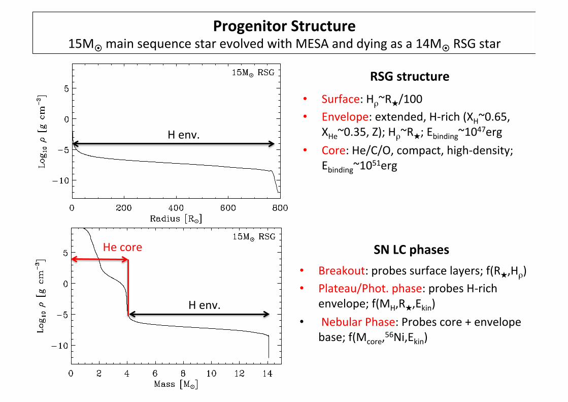
Progenitor  Structure  15M¤  main  sequence  star  evolved  with  MESA  and  dying  as  a  14M¤  RSG  star!

•  Breakout:  probes  surface  layers;  f(R★,Hρ)  •  Plateau/Phot.  phase:  probes  H-­‐rich  

envelope;  f(MH,R★,Ekin)  •   Nebular  Phase:  Probes  core  +  envelope  

base;  f(Mcore,56Ni,Ekin)  

H  env.  

He  core  

H  env.  

•  Surface:  Hρ~R★/100  •  Envelope:  extended,  H-­‐rich  (XH~0.65,  

XHe~0.35,  Z);  Hρ~R★;  Ebinding~1047erg  •  Core:  He/C/O,  compact,  high-­‐density;  

Ebinding~1051erg  

RSG  structure  

SN  LC  phases  

Ejecta  Structure  15M¤  main  sequence  star  evolved  with  MESA  and  dying  as  a  14M¤  RSG  star!

SN  II-­‐P  

He/C/O/56Ni  core  at  V<1500km/s  Small  ekin,  «  arbitrary  »  mass  

Bulk  of  H-­‐envelope  at    2000km/s  <  V  <  5000km/s  

Mass/Velocity  structure  at  homology  

Few  1%  of  Mejecta  at    V>5000km/s  

High  ekin,  small  mass  

Simula%ons  of  SNe  II-­‐P  based  on  15  and  25M¤  progenitor  stars  

•  Phot.  In  outer  ejecta  for  1  month  •  Plateau  probes  H-­‐rich  envelope!  •  Lbol  drops  when  phot.  @H-­‐env.  base  

Inputs:    1.2B  ejecta  from  15/25M!      (830/1100R¤  RSG  progs.)    (evolu%on/explosion  with  kepler)!

•  SN  II-­‐P  LC  morphology  reproduced  •  120d  plateau  for  15M¤  progenitor  •  Nebular  luminosity  =  decay  power  

CCSN  light  curves:  Influence  of  large  varia%ons  in  R★  

R★ :  key  parameter  for  expansion  cooling  Big  stars    (RSG)  =>  SNe  II-­‐Plateau.  Lbol  func%on  of  Eexpl  Small  stars  (WR)  =>  SN  IIb/Ib/Ic.  Lbol  func%on  of  M(56Ni)  

 

0 50 100 150 200 250 300Days since Explosion

1041

1042

1043

Bol

omet

ric

Lum

inos

ity

[erg

s�1 ]

R?=800R�, E=1051erg, M=10M�

R?=R�, E=1051erg, M=5M�

R?=R�, E=1052erg, M=8M�

0 50 100 150 200Days since explosion

�19

�18

�17

�16

�15

�14

�13

Abs

olut

eV-

band

Mag

nitu

de

Ic-BLIcIbIIbIIP

Observa1ons  

Models  

Influence  of  R★  on  Type  II  SN  radia%on  

U-­‐band:  Fast  decline   V-­‐band:  plateau  

•  Test  on  R★ by  adjus%ng  MLT  :    m15mlt1  (R★=1100R¤)  and  m15mlt3  (R★=500R¤)  •  Change  in  R★ affects  the  SN  II  color•  Faster  color  evolu%on  points  to  more  compact  RSG  progenitors    •  Smaller  R★ supported  by  SN  II-­‐P  1999em  observa%ons  •  Property  extends  to  other  SNe  II  (see  also  Gonzalez+15)      

Case  study  of  SNII-­‐P  1999em    1.2x1051erg  ejecta  from                        500R¤  15M¤    RSG.  

Dessart  &  Hillier  (2011),  Dessart+13  

•  Good  match  to  SED,  line  profiles,  ionisa%on  •  Non-­‐thermal  processes  key  for  Hα  at  late  %mes  •  Nebular  spectra  OK  =>  Core  proper%es  suitable  •  LC  OK  for  colors  but  plateau  too  long  –  M(H-­‐env.)    •  Smaller  progenitor  R★:  OK  with  RSG  studies  (Davies+)  

The  peak  blueshiq  of  P-­‐Cygni  profiles  (Anderson+14)  6 Anderson, Dessart et al.

Figure 5. Evolution of the Hα spectral region from 11 d (bottom curve) until 138 d (top curve) after explosion in the SN II-P model m15mlt3 (Dessart et al.2013). The abscissa is the Doppler velocity with respect to Hα. Individual times are color coded, and the time difference between consecutive models is10% of the current time. The two broken lines track the location of maximum absorption and peak emission in Hα. The peak blueshift, strong at early times,decreases as the spectrum formation region recedes, and eventually becomes zero at the end of the plateau phase (in this model at ∼ 140 d).

Figure 5 shows the evolution of the Hα region from 11 d until138 d after explosion in model m15mlt3. This model matcheswell the spectral and light curve evolution of SN 1999em, exceptfor a prolonged plateau phase of ∼<150 d, which stems for theunderestimated RSG mass loss in the MESA model (see Dessartet al. 2013 for details). The evolution of the velocity offset of peakemission agrees qualitatively and quantitatively with the observa-tions. Importantly, all the simulations presented in Dessart et al.(2013) show the same behaviour, in agreement with observations(Fig. 6). Typical peak blueshifts are on the order of −3200 kms−1 at 10 d after explosion and steadily decrease in strength to

eventually reach zero at the end of the plateau, as observed.

5 DISCUSSION

In previous sections it has been shown that significant blue-shiftedvelocities of Hα emission peaks are a common feature of both ob-servations and models of SNe II. Here we first discuss the physicalorigin of these features and their diversity, before presenting two

c⃝ 2012 RAS, MNRAS 000, 1–10

           Hα    

Blue shifted emission peaks in SNe II 5

Figure 4. Evolution in time of the velocity offset of SN Hα emission peaks for the 95 SNe II in the current sample. Three events are shown: a sub-luminousevent, SN 2008bk; a prototype type II-P, SN 1999em; and a faster declining event, SN 2008if. A standard error bar for all measurements is given in black,where the origin of the velocity error is outlined in § 2, and the time error is based on average errors of estimated explosion epochs (see Anderson et al.submitted, for a detailed description of that process).

In the present paper, we inspect the simulations of Dessartet al. (2013), with a special focus on the evolution of line profilemorphology from early photospheric epochs to the onset of the neb-ular phase. We focus on a representative sample of models, namelys15N, m15r1, m15r2, m15os m15mlt1, m15mlt3, m15, m15e3p0,m15e0p6, and m15Mdot (see Dessart et al. 2013 for details; thesemodels cover a range of properties for the same main-sequence starmass but different initial rotation rate, mixing-length parameter,core overshooting prescription, or explosion energy). We also in-clude model m15mlt1x3, which is evolved the same way as m15 butwith a mixing-length-parameter of 1.5 and a mass loss enhanced

by a factor of three compared to the standard red-supergiant (RSG)mass loss rates provided by the ‘DUTCH’ recipe in MESA. Thisproduces a low envelope-mass RSG at the time of explosion, which,when exploded to yield a 1.2 B ejecta kinetic energy, yields a TypeII-Linear light-curve morphology (see Hillier et al., in prep.).

4.2 Results for SN II-P simulations

The first important result is that the peak-emission blueshift,observed in spectra of SNe II (see, e.g., Fig. 1) is also predictedby simulations at all times prior to the onset of the nebular phase.

c⃝ 2012 RAS, MNRAS 000, 1–10

Blue shifted emission peaks in SNe II 7

Figure 6. Evolution of the velocity offset of Hα peak emission with respect to rest wavelength for the large set of models presented in Dessart et al. (2013).All models follow the same trajectory, except for models m15e3p0/m15e0p6 (3 and 0.6 B, respectively), which have a larger/lower ejecta energy than othermodels (i.e., 1.2 B), and for model m15mlt1x3, in which the RSG mass loss was artificially increased by a factor of 3. [See text for discussion].

correlations of this property with other SNe II transient measure-ments.

5.1 The physical origin of blue-shifted emission peaks

In contrast to Chugai (1988), the origin of peak-emission blueshiftseems to stem fundamentally from the steep density profile thatcharacterizes SN ejecta layers, which were originally part of the H-rich envelope. In our simulations, this density distribution is wellrepresented above ∼ 2000 km s−1 (which is roughly where theouter edge of the former He-core lies in 1.2 B explosions of 15 M⊙

RSG stars; Dessart et al. 2010) by a power law ρ(v) ∝ 1/vn,with exponent n on the order of 8. As a consequence, line emissiontends to be confined in space, and subject to strong occultation ef-fects for a distant observer. Instead of coming predominantly fromthe regions with large impact parameter p relative to the photo-spheric radius Rphot the bulk of the emission arises from rays withp < Rphot, i.e. impacting the photo-disk limited by p = Rphot.As explained in Dessart & Hillier (2005b), the line source functiontends to exceed the continuum source function at the continuumphotosphere, naturally leading to line emission above the contin-uum flux level. Because electron-scattering dominates the opacity,line photons have a relatively low destruction probability and we

can therefore see line emission from layers deeper than the contin-uum photosphere.

Fig. 7 illustrates these effects for model m15mlt3 at 11 d (leftpanel). As time progresses, the situation evolves significantly forseveral reasons. The spectrum formation recedes to deeper layersin the ejecta, where the density profile is flatter, favouring extendedemission above the continuum photosphere. The velocities are alsolower, so any velocity offset becomes less conspicuous. More-over, time-dependent ionization exacerbates this effect by mak-ing the line optical depth more slowly varying with radius/velocity(Dessart & Hillier 2008), also favouring extended line emission. In-terestingly, it is in part the increase in the extension of the spectrumformation region that favours the rise of polarization at the end ofthe plateau phase in SNe II-P (Dessart & Hillier 2011).

Departures from the mean trajectory of the peak location invelocity space of emission peaks are visible for three models inFig. 6. First, the two models with a lower/higher kinetic energies(models m15e0p6 and m15e3p0) show smaller/larger offsets, sim-ply reflecting the contrast in ejecta velocity (same envelope massM , but different kinetic energy E). In these, the peak blueshiftsat 10 d after explosion are −2000 km s−1 and −3500 km s−1 re-spectively. Second, model m15mlt1x3, which has a higher ejectakinetic energy to ejecta mass (same E of 1.2 B as the models of

c⃝ 2012 RAS, MNRAS 000, 1–10

Observa1ons  

Models  

Origin  of  the  range  in  SN  II  Luminosity  Signature  of  Explosion  energy?  

ScaEer  of  3mag  in  SN  II  brightness  Fainter  SNe  II  have  narrower  lines  =>  Lower  Ekin  and/or  higher  Mejecta  

A study of low-energy type II supernovaeS. M. Lisakov1*, L. Dessart1, J. D. Hillier2, R. Waldman3, E. Livne3

1 Observatoire de la Côte d’Azur, Nice, France 2 University of Pittsburgh, USA 3 Racah Institute, Jerusalim, Israel* sergey.lisakov@oca.eu

IntroductionThe diversity of observed properties of SNe IIsuggests a range of progenitor mass, radii, butalso explosion energy. We have performed alarge grid of simulations designed to cover thisrange of progenitor and explosion properties. Us-ing MESA STAR, we compute a set of massivestar models (12–30 solar masses) from the mainsequence until core collapse. We then generateexplosions with V1D to produce ejecta within arange of explosion energies and yields. Finally,all ejecta are evolved with CMFGEN to generatemulti-band light curves and spectra. Such low-energy explosions, characterized by low ejectaexpansion rates, are more suitable for reliablespectral line identifications.

SN data setUnlike normal SN IIP low-luminosity ones haveapproximately 10 times less explosion energy(e.g. ⇠ 1050 instead of ⇠ 1051 ergs); amountof ejected 56Ni is small: ⇠ 10�2 M�; expansionvelocities are small (down to ⇠ 103 km/s).

There are two reasons why SN could have lowenergy. It could be either intrinsically low ener-getic explosion of moderate mass (⇠ 8-12M�)star or low-energy explosion of a high mass (⇠25M� and greater), in which large amount ofstellar material remains bound to the core afterthe collapse, and falls back onto it, increasing itsmass [5].

Figure 1: Light curves for low-energey type II su-pernovae and comparison to «normal» type II SN1999em.

References[1] Hillier D. J., Miller D. L., 1998, Astrophysical Journal,

496, 407

[2] Dessart L., Hillier D. J., 2005, Astrophysical Journal,437, 667

[3] Dessart L., Hillier D. J., 2008, Monthly Notices of theRAS, 383, 57

[4] Hillier D. J., Dessart L., 2012, Monthly Notices of theRAS, 424, 252

[5] Zampieri L., Colpi M., Shapiro S. L., Wasserman I.,1998, Astrophysical Journal, 505, 876

A comparison between models and dataSpectrae and light curves has been calculated with CMFGEN code [1, 2, 3, 4]. Model names have thefollowing structure: m12 stands for 12 M�, last letter stands for the explosion energy: t correspondsto 0.3 B, z to 0.6 B, y to 0.9 B, x to 1.2 B, where 1 B (Bethe) = 1051 ergs.We have calculated models for 12, 14, 16, 18, 20, 25 and 27 M�, with different explosion energies. Allthe models have solar metallicity.

Figure 2: Left: selected lines contribution for the model m12z, 14–180 days after explosion. CMFGEN can cal-culate the spectra without a certain element. The difference between the spectra without hydrogen and the spectrawith it gives us an idea of hydrogen contribution. Right: Photospheric velocity of low-luminosity Type II SNededuced from the minima of P-Cygni absorbtion of H↵ line and comparison with some models and «normal» SNtype II 1999em. Lines are models and markers are SNe.

Figure 3: Comparison between model and data multi-band light curves. In the left plot SN 2008bk with excellentobservational data is compared with the model sn08bk1a (xx M�, 0.4⇥1051 ergs explosion). In the right plot SN1999em is compared to the more energetic model m12x.

Figure 4: Spectrae of SN 2008bk and model sn08bk1a (left); Spectrae of SN 2003Z and model m12z (right).

Conclusions. Spectra and light curves of low-energy explosions are very similar. Since low expansionvelocities mean narrow lines, this type of objects is a good subject to exploration.

(S.  Lisakov  poster  FM16p.05)  

Study  of  the  low-­‐luminosity  SN  II-­‐P  2008bk  

Progenitor:  12M¤  MS  star  that  dies  as  a  500R¤ RSG  progenitor  star  at  Z¤  Explosion  model  :  ejecta  with  8.3M¤,  2.5x1050erg  and  0.008M¤  of  56Ni.      Supports  Weak  explosion  in  a  low-­‐mass  RSG  OK  with  progenitor  iden1fica1on  (8-­‐13M¤;  Maund+,  vanDyk+,  Magla+)  

2000 4000 6000 8000 10000 12000λobs [A]

0

1

2

3

4

5

6

7

ObservedF λ+Const.

18d

∆M= 0.7

31d

∆M= 0.7

46d

∆M= 0.7

51d

∆M= 0.7

68d

∆M= 0.7*

82d

∆M= 0.6

97d

∆M= 0.5*

sn08bk4SN2008bk  Model  

0 50 100 150 200 250MJD - 54550.0

�20

�18

�16

�14

�12

�10

�8

�6

Abs

olut

eM

agni

tude

sn2008bksn08bk4(solid)

DM =0.7mag

U +3 B +1.5 V R-1.5 I-3.0

SN2008bk:  symbol  Model:  solid  

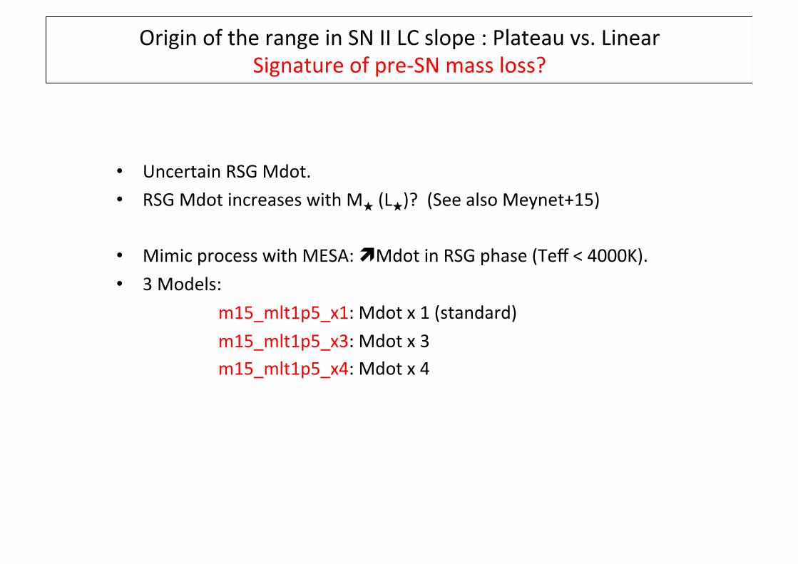
Origin  of  the  range  in  SN  II  LC  slope  :  Plateau  vs.  Linear  Signature  of  pre-­‐SN  mass  loss?  

•  Uncertain  RSG  Mdot.  •  RSG  Mdot  increases  with  M★  (L★)?    (See  also  Meynet+15)  

•  Mimic  process  with  MESA:  ìMdot  in  RSG  phase  (Teff  <  4000K).    •  3  Models:                                                  m15_mlt1p5_x1:  Mdot  x  1  (standard)                                                m15_mlt1p5_x3:  Mdot  x  3                                                m15_mlt1p5_x4:  Mdot  x  4  

Origin  of  the  range  in  SN  II  LC  slope  :  Plateau  vs.  Linear  Signature  of  pre-­‐SN  mass  loss?  

Produces  RSG  at  collapse  with  same  envelope  composi%on  and  R★ but  :  1)  different  H-­‐envelope  mass    2)  Different  H-­‐envelope  density    

Origin  of  the  range  in  SN  II  LC  slope  :  Plateau  vs.  Linear  Signature  of  pre-­‐SN  mass  loss?  

•  Explosions  with  V1D:  Fixed  1.2B  ejecta  

•  Ejecta  +  radia%on  evolu%on  computed  with  CMFGEN  

 

SN  II-­‐P  

SN  II-­‐L  

Progression  from  II-­‐P  to  II-­‐L  Linear  LCS  are  brigher  (same  E!)  Transi%on  %me  to  nebular  phase  f(M)  

Constraints  on  progenitor  masses  

•  MS  mass  ≠  Ejecta  mass  •  Ejecta  mass  func%on  of  pre-­‐SN  mass  loss  &  remnant  mass.                Two  Diagnos%cs:  •  Nebular  spectra  constrain  He  core  mass.                              Two  ways:  kinema1cs  and  line  fluxes    •  SN  LC  constrain  H-­‐envelope  mass  

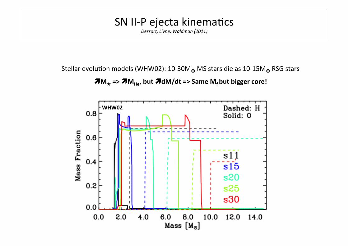
SN  II-­‐P  ejecta  kinema%cs  Dessart,  Livne,  Waldman  (2011)  

Stellar  evolu%on  models  (WHW02):  10-­‐30M¤  MS  stars  die  as  10-­‐15M¤  RSG  stars  

"M★  =>  "MHe,  but  "dM/dt  =>  Same  Mf  but  bigger  core!  

 

WHW02  

SN  II-­‐P  ejecta  kinema%cs:  Vphot  vs.  [OI]  width  Dessart,  Livne,  Waldman  (2011)  

⇒  Higher-­‐mass  progenitors  eject  oxygen  at  a  larger  V  

⇒  V(O)  =500-­‐3000km/s    for  11-­‐30M¤  MS  star  

⇒  Nebular  Observa%ons:  V(OI)  <  1500km/s  =>  MMS  <  20M¤

Constraints  on  progenitor  mass  from  nebular  studies  

•  Explosion  models  +  non-­‐LTE  radia%ve-­‐transfer  modelling.    •  Emission  probes  progenitor  core  +  H-­‐rich  envelope    •  Strong  forbidden  lines  of  FeI/FeII,  OI,  CaII  +  Hα,  NaID,    CaII8500A  •  Abundance  es%mates  (O,  Mg,  Ca)  constrain  progenitor  mass  =>  Supports  moderate  mass  progenitors  (≈15M¤;  Jerkstrand+12;  Maguire+12)  

A. Jerkstrand et al.: The progenitor mass of the Type IIP supernova SN 2004et from late-time spectral modeling

3000 4000 5000 6000 7000 8000 9000 100000

1

2

3

4

5

6

7

8

λ [Å]

Fλ [1

0−15 e

rg s

−1 c

m−2

Å−1

] SN 2004et 401d

12 Msun

model

19 Msun

model

[O I]

Hα

[Ca II]

Ca II

[Fe II]

Na IMg I] [C I]

Fig. 6. Optical (dereddened) spectrum at 401 days (red) compared to the 12 M⊙ (blue) and 19 M⊙ (green) models.

0

2

4

6

8

212 days SN 2004et

15 Msun

model

0

0.2

0.4

0.6

Fλ [1

0−14 e

rg s

−1 c

m−2

Å−1

]

401 days

3000 4000 5000 6000 7000 8000 9000 100000

0.1

0.2

λ [Å]

465 days

Fig. 7. Observed (dereddened) spectra (red) and 15 M⊙ model spectra at 212, 401, and 465 days (black). All spectra have been smoothed with aGaussian of FWHM = 600 km s−1 to improve the S/N.

The observed spectrum shows fluxes in these lines that fall inbetween the 12 M⊙ and 19 M⊙ models.

Also Hα, [Ca II] λλ7291, 7323, and the Ca II IR triplet fluxesdiffer between the models, although by less. These lines aremainly formed in the hydrogen zone, and are therefore not di-rect indicators of the core mass, but rather depend on the quiteuncertain pre-SN mass loss and the explosive mixing.

The spectrum below 6000 Å is a complex mix of mainlyiron-group lines formed by scattering and fluorescence in the hy-drogen envelope. Because of the similar envelopes in the mod-els, the model spectra differ by little in this spectral region. Oneexception is the Mg I] λ4571 line, which arises from the metalcore.

The 15 M⊙ model spectra at 212, 401, and 465 days are plot-ted in Fig. 7. We see that this model is generally successful in re-producing the observed spectra, and in particular reproduces the[O I] λλ6300, 6364 lines well at all epochs. This is further cor-roborated by Fig. 8, where we plot the evolution of Mg I] λ4571,

Na I λλ5890, 5896, [O I] λλ6300, 6364, [Ne II] λ12.81 µm, Hα,[Fe II] λλ7155, 7172, [Ca II] λλ7291, 7323, and the Ca II IRtriplet, from the observed spectra as well as from the three dif-ferent models. Both observed and modeled fluxes have been nor-malized to the bolometric flux of 0.062 M⊙ of 56Co, assuminga distance of 5.5 Mpc. The resulting numbers therefore repre-sent the fraction of the radioactive decay energy re-emerging inthe various lines. The optical line flux measurements were doneby integrating the spectra over Vcut = ±2700 km s−1 and sub-tracting the continuum level, which was taken as the linear in-terpolation of the minimum flux values on the right and lefthandside, within Vcont = ±1.25Vcut = ±3375 km s−1. These veloc-ity limits were found to give reasonable extractions of the linefluxes for all lines and epochs, except for Hα for which we usedVcut = ±7200 km s−1 and Vcont = 1.25Vcut = ±9000 km s−1 to in-clude the broad wings. Because we perform the same operationon model and observed spectra, the choice is not critical for thecomparison.

A28, page 9 of 21

Jerkstrand+12  

Ejecta  mass  inferred  from  LC  modelling  

Radiation hydrodynamics of explosions/eruptions in massive stars 3

This very strict timing of merely a few years, which is orders ofmagnitude smaller than evolutionary or transport timescales, sug-gests a connection between the mechanisms at the origin of thetwo ejections. For SN2006gy, Woosley et al. propose recurrent pair-instability pulsations, a mechanism germane to super-massive starsand therefore extremely rare. For lower mass massive stars, thisshort delay of a few years seems to exclude a very-long, secular,evolution for the production of the first ejection since this wouldhave no natural timing to the comparatively instantaneous event ofcore collapse. Motivated by these recent observations, we explorein this paper whether this diversity of events could be reproducedby a unique and deeply-rooted mechanism, associated with the sud-den energy release above the stellar core and the subsequent shockheating of the progenitor envelope. This means would communi-cate a large energy to the stellar envelope on a shock crossing timescale of days rather than on a very long-diffusion time of thousandsof years or more. Although different in their origin, this energy re-lease could be a weak analogue of what results in pair-instabilitypulsations, i.e. a nuclear flash, as identified in the 8-12M⊙ rangeby Weaver & Woosley (1979).

In this paper, following this shock-heating hypothesis, we use1D radiation-hydrodynamics simulations to explore the productionof explosions/eruptions in stars more massive that ∼10M⊙ on themain sequence. We parameterize the problem through a simple en-ergy deposition, taking place with a given magnitude, over a giventime, and at a given depth in a pre-SN progenitor star. We do notaim at reproducing any specific observation but, through a system-atic approach, try to identify important trends, in a spirit similar tothat of Falk & Arnett (1977). However, we depart from these au-thors by studying “non-standard” explosions. In practice, we con-sider cases where the energy deposited can be both smaller or largerthan the binding energy of the overlying envelope, but must impera-tively be released on a very short time scale to trigger the formationof a shock. Doing so, we identify three regimes, with “standard”SN explosions (short-lived transients) at the high energy end, ob-jects that we will group in the category SN “impostors” (long-livedtransients) at intermediate energy, and variable stars at the very lowenergy end. Let us stress here that we do not make the claim thatall massive-star eruptions, or all transients in general, stem from astrong, sudden, and deeply-rooted energy release in their envelope.Here, we make this our working hypothesis and investigate howmuch such an explosive scenario can explain observations. We dofind that this scenario has great potential and should be consideredas a possibility when examining the origin of massive-star eruptionsand associated transient phenomena.

The paper is structured as follows. In §2, we briefly present thestellar evolutionary models of WHW02 that we use as input for our1D 1-group radiation-hydrodynamics simulations. We discuss theproperties of the progenitor massive stars of WHW02, such as den-sity structure and binding energy, that are relevant for the presentstudy. We then describe in §3, the numerical technique and setupfor our energy deposition study. In §4, we present the results of asequence of simulations based primarily on the 11M⊙ model ofWHW02, discussing the properties of the shocked progenitor en-velope for different values of the strength (§4.1), the depth (§4.2)and the duration (§4.3) of the energy deposition. We also discussin §4.4 the results obtained for more massive pre-SN progenitors,ranging from 15 to 25M⊙ on the main sequence. In §5, we presentsynthetic spectra computed separately with CMFGEN (Hillier &Miller 1998; Dessart & Hillier 2005b; Dessart et al. 2009) for afew models at a representative time after shock breakout. In §6, we

Figure 2.Density distribution as a function of Lagrangian mass at the onsetof collapse for the models of WHW02 evolved at solar metallicity. Noticethe flattening density distribution above the core for increasing mass. Inlow-mass massive stars, the star is structured as a dense inner region (thecore), and a tenuous extended H-rich envelope.

discuss the implications of our results for understanding transientphenomena, and in §7 we summarize our conclusions.

2 INPUT STELLAR EVOLUTIONARYMODELS ANDPHYSICAL CONTEXT

2.1 Input Models

The energy-deposition study presented here starts off from the stel-lar evolutionary calculations of WHW02, who provide a set ofpre-SN massive stars, objects evolved all the way from the mainsequence until the onset of core collapse. We refer the reader toWHW02 for a discussion of the physics included in such models.These physically-consistent models give envelope structures thatobey the equations and principles of stellar structure and evolu-tion. The exact details of these models are not relevant since weaim at developing a general, qualitative, understanding of stellarenvelope behaviour in response to shock-heating - we do not aimat connecting a specific observation to a specific input. Here, wefocus on 10-40M⊙ progenitor stars evolved at solar metallicityand in the absence of rotation. These calculations include the ef-fect of radiation-driven mass loss through a treatment of the outer-boundary mass-flux, so that the final mass in this set reaches amaximum of ∼15M⊙ for a ∼20M⊙ progenitor star. Mass lossleads also to a considerable size reduction of the stellar envelope,with partial or complete loss of the hydrogen rich layers, producingsmaller objects at core collapse for main-sequence masses above∼30M⊙. In the sequence of pre-SN models of WHW02, surfaceradii vary from 4–10×1013 cm in the 10-30M⊙ range, decreasingto ∼ 1011 cm in the 30-40M⊙ range.

The density distribution above the iron core is an importantproperty that distinguishes the structure of massive stars. Low-massmassive stars show a steep density fall-off above their degeneratecore, while the more massive stars boast very flat density profiles(Fig. 2; recall that at the time shown, the Fe or ONeMg core is de-generate and starts to collapse). In the context of core-collapse SNexplosions, this has been recognized as one of the key aspect of theproblem, since this density profile directly connects to the mass-accretion rate onto the proto-neutron star in the critical first sec-ond that follows core bounce (Burrows et al. 2007b). This has led

c⃝ 2009 RAS, MNRAS 000, 1–??

830 V. P. Utrobin and N. N. Chugai: Progenitor of SN 2004et

one-dimensional hydrodynamic modeling of SN 2004et and ingeneral SNe IIP. The progenitor mass of SN 2004et is evalu-ated and compared to estimations for other SNe IIP (Sect. 2.4).The measured progenitor mass noticeably exceeds the mass es-timated from the pre-explosion images, and this disagreementis discussed in Sect. 3.1. In particular, we propose that the ex-plosion asymmetry could be responsible for the disagreement inmass estimates and explore signatures of the explosion asym-metry in the SN 2004et nebular spectra (Sect. 3.2). Finally, inSect. 4, we summarize the results obtained.

We adopt a distance to NGC 6946 of 5.5 Mpc and a redden-ing E(B−V) = 0.41 as measured by Li et al. (2005), an explosiondate on September 22.0 UT (JD 2 453 270.5), and a recessionvelocity to the host galaxy of 45 km s−1 following Sahu et al.(2006).

2. Hydrodynamic model and progenitor mass

2.1. Model overview

The modeling of the SN explosion is performed using thespherically-symmetric hydrodynamic code with one-group ra-diation transfer (Utrobin 2004, 2007), which has been appliedpreviously to other SNe IIP. Utrobin (2007) found that both thisone-group approach and the multi-group approach of Baklanovet al. (2005) measured similar ejecta mass and explosion energyfor SN 1999em. The basic equations and details of the inputphysics, including calculations of mean opacities, are describedin Utrobin (2004). The present version of the code includes ad-ditionally Compton cooling and heating. The explosion energyis modeled by placing the supersonic piston close to the outeredge of the 1.6 M⊙ central core, which is removed from thecomputational mass domain and assumed to collapse to becomea neutron star. The principal limitation of the code is that theexplosion asymmetry and the Rayleigh-Taylor mixing betweenthe helium core and hydrogen envelope (Müller et al. 1991)cannot be correctly treated by the one-dimensional model. We,therefore, study a “non-evolutionary” pre-SN, which takes intoaccount the result of the mixing during the explosion and theshock propagation in the evolutionary pre-SN. The distinctivefeature of the non-evolutionary model is a smoothed density andcomposition jumps between the helium core and the hydrogenenvelope.

The resultant structure of the non-evolutionary pre-SN in ouroptimal model is shown in Fig. 1. The pre-SN model is definedto be a red supergiant (RSG) with a radius of 1500 R⊙, threetimes larger than in the case of the normal type IIP SN 1999em(Utrobin 2007). This large pre-SN radius for SN 2004et is im-plied by the broad initial peak of the bolometric light curveshown by Sahu et al. (2006). The adopted mixing between thehelium core and hydrogen envelope in the optimal model isshown in Fig. 2. The degree of mixing determines the light curveat the end of the plateau (Utrobin et al. 2007). The unmixedhelium-core mass adopted for SN 2004et is 8.1 M⊙, which cor-responds to the final helium core of a main-sequence star of≈25 M⊙ (Hirschi et al. 2004). We note that the model light curveis not sensitive to any variation in the helium-core mass of themixed model (Utrobin et al. 2007).

2.2. Basic parameters

The search for the best-fit model parameters is performed bycomputations of an extensive grid of hydrodynamic models. Theoptimal model should reproduce simultaneously the bolometric

Fig. 1. Density distribution as a function of interior mass a) and ra-dius b) for the optimal pre-SN model. The central core of 1.6 M⊙ isomitted.

Fig. 2. The mass fraction of hydrogen (solid line), helium (long dashedline), CNO elements (short dashed line), and Fe-peak elements includ-ing radioactive 56Ni (dotted line) in the ejecta of the optimal model.

light curve and the photospheric velocity evolution in the bestway. As a result, we derive the ejecta mass Menv = 22.9 ± 1 M⊙,the explosion energy E = (2.3 ± 0.3) × 1051 erg, the pre-SN ra-dius R0 = 1500 ± 140 R⊙, and the 56Ni mass MNi = 0.068 ±0.009 M⊙. The uncertainties in the basic parameters are calcu-lated by assuming relative errors in the input observational data:11% in the distance, 7% in the dust absorption, 5% in the pho-tospheric velocity, and 2% in the plateau duration. In general,the errors of derived parameters should be somewhat larger be-cause of model systematic errors. However, the latter cannot beconfidently estimated unless a more advanced and correct modelis developed. The model uncertainties will be discussed belowin Sect. 3.2.

The density distribution in the freely expanding SN envelopeis shown in Fig. 3. Multiple shells in the outermost layers withvelocities v > 14 000 km s−1 (Fig. 3) form at the shock breakoutstage by the radiative acceleration in the optically thin regime.The origin of these shells is related to the specific behavior of theline opacity in the outer rarefied layers of temperature ∼105 K.The innermost shell of mass ∼5 × 10−3 M⊙ at the velocity of11 700 km s−1 is the thin shell formed by the effect of the shock

830 V. P. Utrobin and N. N. Chugai: Progenitor of SN 2004et

one-dimensional hydrodynamic modeling of SN 2004et and ingeneral SNe IIP. The progenitor mass of SN 2004et is evalu-ated and compared to estimations for other SNe IIP (Sect. 2.4).The measured progenitor mass noticeably exceeds the mass es-timated from the pre-explosion images, and this disagreementis discussed in Sect. 3.1. In particular, we propose that the ex-plosion asymmetry could be responsible for the disagreement inmass estimates and explore signatures of the explosion asym-metry in the SN 2004et nebular spectra (Sect. 3.2). Finally, inSect. 4, we summarize the results obtained.

We adopt a distance to NGC 6946 of 5.5 Mpc and a redden-ing E(B−V) = 0.41 as measured by Li et al. (2005), an explosiondate on September 22.0 UT (JD 2 453 270.5), and a recessionvelocity to the host galaxy of 45 km s−1 following Sahu et al.(2006).

2. Hydrodynamic model and progenitor mass

2.1. Model overview

The modeling of the SN explosion is performed using thespherically-symmetric hydrodynamic code with one-group ra-diation transfer (Utrobin 2004, 2007), which has been appliedpreviously to other SNe IIP. Utrobin (2007) found that both thisone-group approach and the multi-group approach of Baklanovet al. (2005) measured similar ejecta mass and explosion energyfor SN 1999em. The basic equations and details of the inputphysics, including calculations of mean opacities, are describedin Utrobin (2004). The present version of the code includes ad-ditionally Compton cooling and heating. The explosion energyis modeled by placing the supersonic piston close to the outeredge of the 1.6 M⊙ central core, which is removed from thecomputational mass domain and assumed to collapse to becomea neutron star. The principal limitation of the code is that theexplosion asymmetry and the Rayleigh-Taylor mixing betweenthe helium core and hydrogen envelope (Müller et al. 1991)cannot be correctly treated by the one-dimensional model. We,therefore, study a “non-evolutionary” pre-SN, which takes intoaccount the result of the mixing during the explosion and theshock propagation in the evolutionary pre-SN. The distinctivefeature of the non-evolutionary model is a smoothed density andcomposition jumps between the helium core and the hydrogenenvelope.

The resultant structure of the non-evolutionary pre-SN in ouroptimal model is shown in Fig. 1. The pre-SN model is definedto be a red supergiant (RSG) with a radius of 1500 R⊙, threetimes larger than in the case of the normal type IIP SN 1999em(Utrobin 2007). This large pre-SN radius for SN 2004et is im-plied by the broad initial peak of the bolometric light curveshown by Sahu et al. (2006). The adopted mixing between thehelium core and hydrogen envelope in the optimal model isshown in Fig. 2. The degree of mixing determines the light curveat the end of the plateau (Utrobin et al. 2007). The unmixedhelium-core mass adopted for SN 2004et is 8.1 M⊙, which cor-responds to the final helium core of a main-sequence star of≈25 M⊙ (Hirschi et al. 2004). We note that the model light curveis not sensitive to any variation in the helium-core mass of themixed model (Utrobin et al. 2007).

2.2. Basic parameters

The search for the best-fit model parameters is performed bycomputations of an extensive grid of hydrodynamic models. Theoptimal model should reproduce simultaneously the bolometric

Fig. 1. Density distribution as a function of interior mass a) and ra-dius b) for the optimal pre-SN model. The central core of 1.6 M⊙ isomitted.

Fig. 2. The mass fraction of hydrogen (solid line), helium (long dashedline), CNO elements (short dashed line), and Fe-peak elements includ-ing radioactive 56Ni (dotted line) in the ejecta of the optimal model.

light curve and the photospheric velocity evolution in the bestway. As a result, we derive the ejecta mass Menv = 22.9 ± 1 M⊙,the explosion energy E = (2.3 ± 0.3) × 1051 erg, the pre-SN ra-dius R0 = 1500 ± 140 R⊙, and the 56Ni mass MNi = 0.068 ±0.009 M⊙. The uncertainties in the basic parameters are calcu-lated by assuming relative errors in the input observational data:11% in the distance, 7% in the dust absorption, 5% in the pho-tospheric velocity, and 2% in the plateau duration. In general,the errors of derived parameters should be somewhat larger be-cause of model systematic errors. However, the latter cannot beconfidently estimated unless a more advanced and correct modelis developed. The model uncertainties will be discussed belowin Sect. 3.2.

The density distribution in the freely expanding SN envelopeis shown in Fig. 3. Multiple shells in the outermost layers withvelocities v > 14 000 km s−1 (Fig. 3) form at the shock breakoutstage by the radiative acceleration in the optically thin regime.The origin of these shells is related to the specific behavior of theline opacity in the outer rarefied layers of temperature ∼105 K.The innermost shell of mass ∼5 × 10−3 M⊙ at the velocity of11 700 km s−1 is the thin shell formed by the effect of the shock

SN  II-­‐P  LC  modelling  constrains  the  proper%es  of  the  H-­‐env.  =>  NO  constraint  on  the  He  core.  Constraints  on  progenitor  He  core  (mass,  composi%on)  come  from  nebular-­‐phase  spectra!  

SN  2004et  

Larger  progenitor  masses  inferred  from  LC  modelling  (Utrobin+)  than  pre-­‐SN  detec%ons  But  discrepancy  largely  1ed  to  inferred  He-­‐core  mass.  

SN1999em:  Mejecta=19.0M¤  but  MH-­‐env=11M¤  (Utrobin  2007)    SN  2004et:  Mejecta=24.5M¤  but  MH-­‐env=12M¤ (Utrobin  &  Chugai  2009)  =>  H-­‐env  mass  of  ~10M¤  :  OK  for  15M¤  progenitor  

Utrobin+09  

SNe  II-­‐P  as  metallicity  probes  Model  sequences  from  15  to  120d  at  0.1  to  2xZ¤ Sens%vity  to  metal  content  (O,  Na,  Ca,  Ti,  Fe)  

SNe II-P as metallicity probes 3

Table 1. Summary of model properties used as initial conditions for CMFGEN simulations. The first set of models are for different metallicities. The secondset includes solar-metallicity models evolved with different values of the mixing length parameter (models m15mlt2, also referred to as mlt2, and m15z2m2are the same). This second set is used merely to estimate systematic errors in Section 3.

model Z Mfinal Age Teff R⋆ L⋆ MH MHe MO Mr,YeMr,H MH,env Mej Ekin M56Ni

[Z⊙] [M⊙] [Myr] [K] [R⊙] [L⊙] [M⊙] [M⊙] [M⊙] [M⊙] [M⊙] [M⊙] [M⊙] [B] [M⊙]

m15z2m3 0.1 14.92 13.57 4144 524 72890 7.483 5.048 0.507 1.61 4.15 10.77 13.29 1.35 0.081m15z8m3 0.4 14.76 13.34 3813 611 71052 7.183 5.252 0.428 1.63 4.09 10.67 13.12 1.27 0.036m15z2m2 1.0 14.09 12.39 3303 768 63141 6.630 5.105 0.325 1.62 3.88 10.21 12.48 1.27 0.050m15z4m2 2.0 12.60 10.88 3137 804 56412 5.119 5.042 0.387 1.40 3.77 8.83 11.12 1.24 0.095

m15mlt1 1.0 14.01 12.36 3318 1107 106958 6.516 5.167 0.354 1.36 3.89 10.13 12.57 1.24 0.121m15mlt2 1.0 14.09 12.39 3303 768 63141 6.630 5.105 0.325 1.62 3.88 10.21 12.48 1.27 0.050m15mlt3 1.0 14.08 12.41 4106 501 64218 6.542 5.173 0.383 1.54 3.92 10.16 12.52 1.34 0.086

Notes: For the solar composition, we adopt the values of Grevesse & Sauval (1998) and scale each metal mass fraction as indicated. Following the columnscontaining the cumulative ejecta masses in H, He, and O, we give the Lagrangian mass corresponding to specific locations in the pre-SN star. We giveMr,Ye

,which corresponds to the edge of the iron core, i.e., where the electron fraction Ye rises to 0.49 as we progress outward from the star center (this is also thepiston location for the explosion), andMr,H which corresponds to the base of the H-rich envelope (i.e., the helium-core mass). The last three columns givesome ejecta properties that result from the imposed explosion parameters. The quoted 56Ni mass corresponds to that originally produced in the explosion.

Figure 1. Spectral evolution in the optical range for SN II-P models at one-tenth (m15z2m3; left) and twice (m15z4m2; right) the solar metallicity, highlightingtheir sensitivity to metallicity variations. The UV range is also sensitive to metallicity variations but lines tend to overlap and to be saturated, which complicatesthe analysis. The red curve corresponds to the synthetic continuum flux. Line identifications are discussed in detail in the appendix of Dessart et al. (2013).

c⃝ 2014 RAS, MNRAS 000, 1–11

0.1Z!   2Z!  

Dessart+14  

EW(FeII5018A):  models  vs.    observa%ons  8 L. Dessart, C. P. Gutierrez, M. Hamuy, D. J. Hillier, T. Lanz et al.

Figure 4. Comparison of pEWs between observations (SNe 2007il, 2005J, and 2008ag) and SN II-P models of increasing metallicity (0.4, 1, 2 times solarfrom left to right). The same measurement procedure is used on observed and synthetic spectra.

Figure 5.Montage of spectra for the three SNe II-P shown in Fig. 4. The time is ∼ 80 d after explosion.

els, the evolution through the plateau phase leads to a systematicincrease in the magnitude of these EWs. Hα shows little sensitivityto metallicity, while Na I D becomes markedly weaker only whenthe metallicity is decreased to one-tenth solar. However, O I 7777 A,Fe II 5169 A, and Fe II 5018 A exhibit a systematic trend at all timesthat correlates with the metallicity of the model. A good time foranalysis is during the recombination phase, when metal-line blan-keting is strong, but before the end of the plateau to avoid any pollu-tion at the photosphere, as may occur through the mixing of speciesfrom the helium core into the H-rich envelope.

We have confronted the models to a selection of SNe II-P fromthe CSP and former followup programs (Hamuy et al. 2006; An-derson et al. 2014). Calculating pseudo-EWs on both observationsand models at the recombination epoch, we find they exhibit thesame behavior from the early-photospheric phase until the end ofthe plateau (e.g., increasing EW magnitude in Fe II 5018 A). Com-paring the measurements at ∼ 80 d after explosion, we find that allselected SNe fall within the pEW limits set by the 0.4 and 2×Z⊙

models. No SN II-P in our sample matches the weak metal-linestrengths of our model at Z⊙/10. Since the CSP observations are

c⃝ 2014 RAS, MNRAS 000, 1–11

SNe II-P as metallicity probes 9

Figure 6.Distribution of data measurements of pEWs for observed SNe II-P and the corresponding tracks of theoretical points for models m15z2m3, m15z8m3,m15z2m2, and m15z4m2 (models at 0.1, 0.4, 1, and 2× Z⊙). Notice the scarcity of standard SNe II-P in the vicinity of the model at one-tenth solar metallicity.For comparison, we also add the location of SN 1999em in this plane (the explosion time for 1999em was inferred by Dessart & Hillier (2006), with an errorof ± 1.0 d).

probably representative of type II SNe, we speculate that we areyet to observe a SN II-P at SMC metallicity in the local Universe.

Our metallicity measurements compare favorably withnebular-line analyses. Such studies, based on both targeted (An-derson et al. 2010) and untargeted (Stoll et al. 2013) surveys con-firm the scarcity of SNe II-P at low metallicity. The absence of lowmetallicity SNe in our sample most likely reflects the paucity ofvery low metallicity systems in the local universe. The absence oflow metallicity hosts is also seen in the analysis of core collapseSNe out to z ∼ 0.2 by Kelly et al. (2014). Since stellar evolutiondepends on metallicity it is important to study SN at low metal-licities. Extreme rotation rates on the main sequence, for example,can prevent a star, if it has an initial mass of

∼> 20M⊙, from evolv-

ing to the red and from exploding as a RSG (see, e.g., Brott et al.2011). Irrespective of rotation, stars in the mass range 10–20M⊙

are expected to explode in a RSG phase at low metallicity, and thusshould be seen.

In addition to providing important constraints on the SN andits progenitor, quantitative spectroscopy of SNe can also be used

for determining the evolution of metallicity with redshift, and forrevealing the metallicity distribution with galactocentric radius.The high luminosity of SNe makes them ideal substitutes to stars(see, e.g., Kudritzki et al. 2012), but may also offer an alterna-tive to nebular-line analyses (Osterbrock 1989; Kewley & Dopita2002; Pettini & Pagel 2004). At very large distances, we will needsuper-luminous SNe resulting from the pair-production instabil-ity in a super-massive RSG-star, since their plateau luminositiesare predicted to be on the order of 1010 rather than a few 108 L⊙

(Kasen et al. 2011; Dessart et al. 2013). Unfortunately, such super-luminous SN II-P events are yet to be discovered.

With VLT-FORS, a SN II-P of 14th magnitude at 10Mpc re-quires a 0.7 s exposure to yield a S/N of 30 per pixel (grism 150I).At 100Mpc, this exposure time is 70 s. Using a Hubble constant of70 km s−1Mpc−1, that same SN at a redshift of 0.1 would requirean exposure of about 30min for the same setup. With the futureextremely-large telescopes, going up to redshift one and beyondmay be possible. In practice, to reduce systematic errors from themodeling and to circumvent inaccurate pseudo-equivalent widths

c⃝ 2014 RAS, MNRAS 000, 1–11

•  ScaEer  %ed  to  varia%ons  not  just  in  Z,  but  also  in  M★,  R★,  Eexpl  etc.  

•  Lack  of  low  Z  progenitors  

Conclusions  •  Type  II  SNe  offer  important  complementary  informa%on  on  RSG  stars    

•  Radia%ve  transfer  models  essen%al  for  distant  SNe  II  (no  progenitor  detec%on)  

•  SN  Radia%ve  transfer  modelling  key  tool  to  constrain  RSG  interior,  He  core  mass  etc  

•  Photospheric  phase:  Constraints  on  H-­‐envelope  (Xi,  v(m),  ioniza%on,  Reddening…)  

•  Nebular  phase:  Constraints  on  He-­‐core  (yields)  

⇒  V-­‐band  plateau  &  U-­‐band  fading  =>  R★  ≤500R¤ ⇒  LC  diversity  reflects  varia%ons  in  R★,  M(H-­‐env),  Eexpl,    M(56Ni)  

•  Low-­‐L  SNe  II-­‐P:  OK  with  low-­‐mass  progenitor    

•  SN  II-­‐P  versus  II-­‐L:  varia%ons  in  E/M?  Connec%on  to  pre-­‐SN  mass  loss •  Mass  discrepancy:  Primarily  associated  with  large  core  masses  which  are  NOT  constrained  by  

LC  modeling.  All  OK  with  ~15M¤  prog.  within  uncertain%es.  

•  SN  II-­‐P  as  metallicity  probes.  Lack  of  low-­‐Z  SNe  II-­‐P  in  current  sample.