radio amateur exam - qsl.net · radio amateur exam general class by 4s7vj chapter-6 transmission...

RAE-Lessons by 4S7VJ

1

RADIO AMATEUR EXAM

GENERAL CLASS

By 4S7VJ

CHAPTER-6

TRANSMISSION LINES AND ANTENNAS

6.1 Transmission line

There are three separate parts are involved in an

antenna system;

1. The radiator (antenna)

2. Transmission line (Feed line)

3. Coupling arrangement (antenna tuner)

The place where RF power is generated is very

frequently not the place where it is to be utilized. The

antenna to radiate well, should be high above the ground

and should be keep clear of trees and other obstacles

that might absorb energy, but the transmitter itself is

most conveniently installed indoor where it is readily

accessible. The transmission line used to connect the

antenna to the TX or Rx with a minimum of loss due to

resistance or radiation. By the use of transmission lines

or feeders, the power of the TX can be carried

appreciable distance without much loss due to conductor

resistance, insulator losses or radiation.

Types of Transmission line

There are three main types of transmission lines.

(1) The single wire feed arranged so that there is a

true traveling wave on it.

(2) The parallel wire line with two conductors

carrying equal but oppositely directed current

and voltages, is balanced with respect to earth.

(3) The coaxial or concentric line in which the outer

conductor enclosed the inner conductor.

6.1.1 Single wire feeder

Single wire feeders are inefficient and now

seldom used since it is impossible to prevent them

acting to some extent as radiators, and the return

path which is via the ground, introduced further

losses. The feeder wire itself also acting as the

antenna.


2

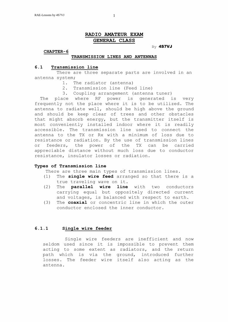
6.1.2 Parallel wire line This is called as a balanced line or open wire

line. There are two types, two open parallel wires

separated by insulating spreaders, and the other type

is twin-lead, in which the wires are embedded in solid

formed insulation. The field is confined to the

immediate vicinity of the conductor and there is

negligible radiation (losses), if proper precautions

are taken. Line losses results from Ohmic resistance,

radiation from the line and deficiencies in the

insulation. Large conductors, closely spaced in terms

of wavelength, and using a minimum of insulation, make

the best balanced line. Balanced lines are best in

straight runs. If bends are unavoidable, the angle

should be as obtuse (between 90 and 180) as possible. Care should be prevent one wire from coming closer to

metal object than the other. Wire spacing should be

less than 1/20 of wavelength.

Fig-6.1

Properly build open-wire line can operate with

very low loss in VHF and even UHF installations. A

total line loss under 2dB per 100ft at 432MHz is

readily obtained. A similar 144MHz setup (2 meter

band) could have a line loss under 1dB per 100ft.

6.1.3 Coaxial line Coaxial or concentric line made out of two

cylindrical

conductors having a common axis. The space between two

conductors is filled with an insulating material; may

be a solid or air. In the coaxial line the current

passes along the center conductor and returns along the

inside of the sheath or braid. Due to skin effect at

high frequencies the current do not penetrate more than

a few micro meters into the metal; hence with any

practical thickness of the sheath there is no current

on the outside. The fields are thus held inside the

cable and cannot radiate.


3

6.1.4 Characteristic Impedance of a transmission line

If the transmission line were infinitely long and

free from losses a signal applied to the input end would

travel on for ever, energy being drawn away from the

source of signal just as if a resistance had been

connected instead of the infinite line. This resistance

is known as the Characteristic Impedance of the line and

usually denoted by the symbol “Zo”. If we replace the

line with pure resistance of Zo the generator will not be

aware of any change. There is still no reflection, all

the power applied to the input end of the line is

absorbed in the terminating resistance, and the line is

said to be matched.

A transmission line can be considered as a long ladder

network of series inductances and shunt capacitances,

corresponding to the inductance of the wires and the

capacitance between them. It differs from conventional L-

C circuits in that these properties are uniformly

distributed along the line. If the inductance and

capacitance for any particular length are L and C then

the characteristic impedance Zo given by:

Zo = (L/C) Ohms

(If “L” in Henrys and “C” in Farads then “Zo” is in Ohms

and also “L” in micro Henrys and “C” in micro Farads then

“Zo” is in Ohms.)

N.B.:-

Almost every book says the value of “L” and “C” are the

inductance and capacitance for a unit length of the

coaxial cable but it is not true, any length is suitable,

and also there is no difference between straight cable or

coiled form according to my practical experience.

Fig 6.2


4

6.1.4.1 Characteristic impedance of a parallel wire line

Suppose the radius of the cross section of each wire

is “r” and the distance between two axis’s is “s” then

the characteristic impedance:

Zo = 276 Log(s/r) Ohms

6.1.4.2 Characteristic impedance of a coaxial line

Suppose the diameters of outer conductor and inner

conductor respectively “D” and “d” then the

characteristic impedance of an air core coaxial line:-

Zo = 138 Log(D/d) Ohms

6.1.4.3 How to Measure the Characteristic Impedance

Capacitance “C”

First you take a coaxial cable having several meters

long. Keep both ends open. Measure the capacitance

between centre conductor and the braid with using a

capacitance meter(digital multimeter) or DIP meter. (Fig.

6.3)

Inductance “L”

Then short circuit one end of the cable, and measure

the inductance between the centre conductor and the braid

of the other end by using an inductance meter (digital

multimeter) or with a DIP-meter. (Fig. 6.3)

Fig 6.3

Now calculate Z0 according to this formula, Z0 =√(L/C).


5

6.1.5 Velocity Factor

When the medium between the conductors of a

transmission line is air, the traveling waves will

propagate along it at the same speed as waves in free

space. If a dielectric material is introduced between the

conductors for insulation or support purposes, the waves

will be slowed down.

The ratio of the velocity of the waves on the line to

the velocity in free space is known as the velocity

factor. It is approximately 0.66 for solid polythene

cables. For open wire lines, it is between 0.8 and 0.95,

while open wire lines with spacers at intervals may reach

0.98. It is important to make proper allowances for this

factor in some feeder applications.

For example if velocity factor is 2/3 (or 0.66) then

quarter wave line would be physically 1/6 wavelength

long. ( 2/3 x 1/4 = 1/6)

Velocity factor for RG8A/U, RG58 and RG213/U coaxial

cables is 0.66.

Example:-

Calculate the half wave lengths of 145.550MHz for

following conditions.

1. in the free space

2. thin antenna wire

3. RG58 coaxial cable

solution:-

1. in the free space,

wave length = 300/frequency(MHz)

= 300/145.550

= 2.061m

half wave length = 2.061/2

= 1.0305m = 103.05cm

2. For thin antenna wire,

velocity factor for thin wire is approximately 0.95

therefore half wave length = 0.95 x ½ x 300/145.55

= 0.979m = 97.9cm

3. RG58 coaxial cable

velocity factor for RG58 cable is about 0.66

therefore half wave length = 0.66 x ½ x 300/145.55

= 0.6801m = 68.01cm

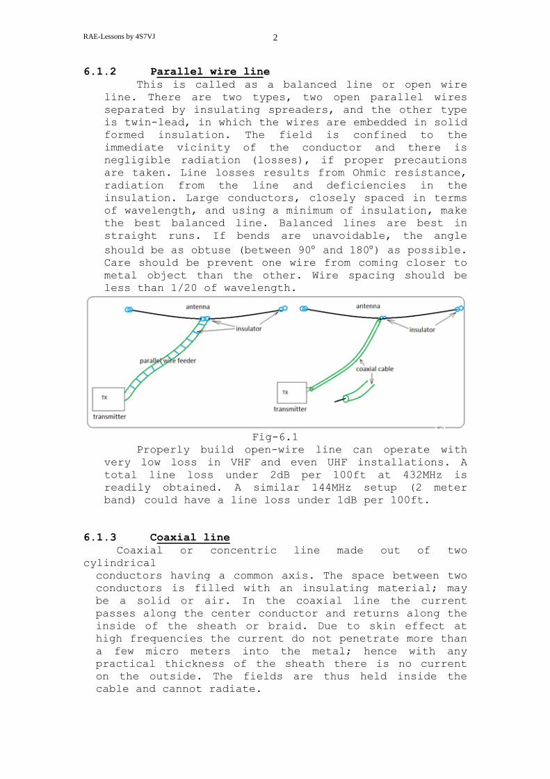
6.1.5.1 Measuring of electrical length

We can measure the

resonance frequency for ½

wave length or ¼ wave length

by using a dip meter.

According to the diagram in

Fig 6.4 connect one turn of

Fig-6.4


6

a coil to one end of the coaxial cable. If the other end is

short circuit, the length is equal to the electrical ½ wave

length for the resonance frequency.

If the other end is open circuit, the length is equal

to the electrical ¼ wave length for the resonance

frequency.

6.1.6 Standing waves

When a transmission line terminated by a resistance

equal in value to its characteristics impedance, there is

no reflection and the line carries a pure traveling wave.

When the line is not correctly terminated, the voltage to

current ratio is not the same for the load as for the

line and the power fed along the line cannot all be

absorbed to the load, some of it is reflected in the form

of a secondary traveling wave, which must return along

the line. These two waves, forward and reflected,

interact all along the line to setup a standing wave.

6.1.7 Standing Wave Ratio – SWR

For get the maximum efficiency of a transmission

line the characteristic impedance of the line (Zo) should

be equal to the characteristic impedance of the antenna

(Z).

Standing wave ratio or SWR is a figure which can be

measure the amount of mismatch of the antenna system.

This is always equal or greater than 1. SWR = 1 for a

perfectly matched antenna system.

SWR = Zo/Z or Z/Zo (which ever is greater)

Example:

A transmission line having a characteristic

impedance of 50 and terminating to an antenna having

40 radiation resistance. What is the SWR of the antenna system?

Solution:

Z0 = 50 and Z = 40

SWR = Z0 / Z

= 50/40

= 1.25

If the line is not perfectly match, there is a standing

wave along the transmission line. Therefore the voltage

and the current is varying according to the standing

wave. Then the ratio between the maximum and minimum


7

value of current or voltage is equal to the SWR. Refer

the diagram (Fig.6.5)

SWR = Imax/Imin

= Vmax/Vmin

If the transmission line is perfectly matched to the

antenna, the voltage or current through the line is

constant and SWR = 1

Example:

The maximum and minimum voltages along a

transmission line are 180 and 100 respectively. What is

the SWR of the system.

Solution:

SWR = Vmax/Vmin , Vmax = 180v, Vmin = 100v

= 180/100 = 1.8

Fig 6.5

Measure the SWR according to the above explanation is not

practicable because no way to measure these values.

6.1.7.1 SWR METER

This is a simple instrument use for measure SWR of a

transmission line. Every shack should have one SWR meter.

It can be the first indicator of antenna trouble. Fig 6.6

shows the circuit diagram for a simple SWR meter. ( Refer

paragraph 7.2.1 in the chapter-7 for calibration detail)

There is a special type of SWR meter use for visually

handicaps. In this instrument generates an audio tone,

the frequency of the tone is varying according to the

SWR.


8

Fig-6.6

Fig-6.7

6.1.8 Reflection Coefficient

The ratio of the voltage in the reflected wave to

the voltage in the incident wave (forward voltage) is

defined as the reflection Coefficient. This coefficient

is designated by the Greek letter rho ( ρ )

ρ = Vr /Vf Vr = reflected voltage

Vf = forward voltage

ρ = √( Pr /Pf ) Pr = reflected power

Pf = forward power

For perfectly matched transmission line,


9

ρ = 0 because Vr = 0 or Pr = 0

For completely mismatched transmission line,

ρ = 1 because Vr = Vf or Pr = Pf

6.1.9 Relationship between SWR and reflection coefficient

1 + ρ

SWR = --------------

1 – ρ

SWR - 1

ρ = ----------------- SWR + 1

6.1.10 Relationship between SWR and voltage

We can rearrange the above formula with the forward

and reflected voltages as follows:

Vf + Vr

SWR = --------------

Vf - Vr

6.1.11 Relationship between SWR and power

If the forward power and reflected power are

respectively Pf and Pr then we can rearrange the above

formula as follows:

SWR = (√Pf + √Pr )/( √Pf - √Pr )

6.2 ANTENNAS (Aerials)

Introduction

The radio signal passes from one station to another

station as a wave propagating in the atmosphere, but in

order to achieve this it is necessary to have at the

sending end something which will take the power from the

transmitter and launch it as a wave, and at the other

end extract energy from the wave to feed the receiver.

This is an antenna (aerial) and, because the fundamental

action of an antenna is reversible, similar antennas can

be used at both ends. The antenna then is a means of

converting power flowing in wires to energy flowing in a

wave in space, or is simply considered as a coupling

transformer between the wires and free space.


10

Dipole

The most simple and commonly used word in antenna work

is Dipole or simple dipole. Basically a dipole is simply

which has two poles or terminals into which radiation-

producing current flow. Dipole is used as a reference

antenna for antenna experiments.

6.2.1 Properties of Antennas

There are some important properties of antennas as

follows:

1. Resonant 2. Radiation 3. polarization 4. Directivity 5. Gain 6. Radiation resistance

6.2.1.1 Resonance of an Antenna

When the SWR of an antenna is 1 (or 1:1) then the

antenna is perfectly matched, in other word the total RF

power out put is converts to electro magnetic wave or we

can say the antenna is resonating for the particular

frequency. Normally this is happens for the multiple of

half wave lengths of the antenna.

6.2.1.2 Radiation

Whenever a wire carries an alternating current the

electromagnetic wave travel away into the space with the

velocity of light. It is called the radiation of the

electromagnetic energy or RF (radio frequency) energy.

We normally use the antenna as the radiator or radiating

element. The amount of radiation is proportional to the

current flowing into the antenna.

6.2.1.3 Polarization

There are two inseparable fields associated with

the transmitted signal,

1. An electric field due to voltage changes, 2. A magnetic field due to the current changes,

and these always remain at right angles to one another

and to the direction of propagation as the wave

proceeds. The lines of forces in the electric field run

in the plane of the transmitting antenna. By convention

the direction of the lines of forces of the electric

field defines as the direction of polarization or the

plane of polarization of the radio wave.

Thus horizontal antennas propagate horizontal

polarized waves and vertical antennas propagate vertical

polarized waves.


11

For the maximum performance RX antenna also should be

in the same polarization plane. When the TX antenna is

horizontal, RX antenna also should be in the horizontal

plane.

Circular Polarization

For long distance propagation through ionospheric

layers, due to reflection, refraction and diffraction a

degree of cross polarization may be introduced which

results in signals arriving at the receiving antenna

with both horizontal and vertical components presents.

This signal called as circularly polarized. Varying of

the plane of the receiving antenna is not giving any

deference for circular polarized signal.

6.2.1.4 Directivity

The radiation field which surrounds the antenna is

not uniformly strong in all directions. It is strongest

in directions at right angles to the current flow in the

antenna element and falls in intensity to zero along the

axis of the element; in other words its exhibits

directivity in its radiation pattern, the energy being

concentrated in some directions at the expense of

others. Later it will be explained how directivity may

be increased by using number of elements. These are

called beam antennas.

6.2.1.5 Antenna Gain

If one antenna system can be made to concentrate

more radiation in a certain direction than another

antenna (reference antenna), for the same total power

supplied, then it is said to exhibit gain over the

second antenna in that direction. In other words, more

power would have to be supplied to the reference antenna

to give the same radiated signal in the direction under

the consideration.

Gain can be expressed either as a ratio of the power

required to be supplied to each antenna to give equal

signals at a distant point, or as the ratio of the

signals received at that point from the two antennas

when they are driven with the same power input. Gain is

usually expressed in decibels, according to the

following formula.

Antenna gain

dB = 10 Log (P2/P1)

where P1 = input power to the directional antenna

P2 = input power to the reference antenna to

exhibit

same performance


12

6.2.1.6 Effective Radiated Power ERP

ERP is the effective radiated power of an antenna

system with respect to a standard radiator or antenna.

Measured antenna performance is usually compared to a

dipole.

For an example:- A transmitter having 15 W out put

power is connected to an antenna system of 6dB gain.

What is the ERP?

Let the ERP = P, therefore 6dB = 10 Log (P/15)

therefore 0.6 = Log (P/15)

but antilog of 0.6 = 4

therefore Log 4 = Log (P/15)

4 = P/15, P = 60

therefore ERP = 60 watts

6.2.1.7 Radiation resistance or antenna impedance

Fig 6.8

When power is delivered from the transmitter into

the antenna, some small part will be lost as heat, since

the material of which the antenna is made will have a

finite resistance, albeit small, and a current flowing


13

in it will dissipate some power. The bulk of the power

will usually be radiated and, since power can only be

consumed by a resistance, it is convenient to consider

the radiated power as dissipated in an imaginary

resistance which is called the radiation resistance of

the antenna.

Using ordinary relationships of circuits, if the

current flow is I into the radiation resistance R then

the power of I2 x R watts is being radiated. ( W = I² R )

The radiation resistance of an antenna is varying with the

height above the ground. Fig 6.8 shows the pattern of

variation for simple dipole. It is approaching to 72 Ohms.

6.2.1.8 Free Space Wave Length

The relation between the wave length and frequency

is very simple. The product of wave length and frequency

is equal to the speed of electro magnetic wave (radio

signal).

v = f x λ

Where, v = speed, f = frequency, λ = wave length, speed

ajnd wave length are depend on the medium which the wave

is traveling. We can assume that the wave is traveling

through air (atmosphere) and free space. Speed of radio

waves (same as speed of light) in the free space and the

air are almost same. It is 299,792,458 m/s (299.792458

Mm/s) in free space. If we take the frequency in MHz and

wave length in meters, then speed is in Mega meters, so

we can write the above formula as

299.792458 (Mm/s) = f (MHz) x λ (m)

or

MHz x meter = 299.792458

Approximately we can consider this as

MHz x meter = 300

6.2.1.9 Field Strength

The RF energy generated by the TX is radiated to the

space by the antenna. This energy density (field

strength) gradually gets reduced because it’s spread into

space. We can calculate the field strength according to

the following formula.

Hear E = field strength (V/m)

P = Effective radiated power (ERP) in watts (W)

d = the distance from the antenna (m)


14

Example :-

A vhf transmitter having 3W output power is connected to

an antenna having 20dB gain. Find the field strength at a

point 100m away from the antenna.

Find the ERP first. According to the formula

dB = 10 Log(Pout /Pin)

therefore 20 = 10 Log(ERP/3)

therefore 2 = Log(ERP/3)

but we know that 2 = Log100

therefore Log100 = Log(ERP/3)

therefore ERP/3 = 100

ERP = 300 Watts

Now apply the formula E = (√30P)/d, P=300, d=100

Therefore E = (√30x300)/100 = √9000 / 100

= 94.8/100

= 0.948 V/m

= 948 mV/m

6.2.2 Types of Antennas

There are various types of antennas for using with

HF, VHF, UHF, and other bands and also with receivers

and transmitters. The following list included several

types.

1. Vertical antenna 2. Long wire (harmonic) 3. Dipole 4. Whip 5. Loop 6. Quad 7. Yagi 8. Quagi 9. Parabolic 10. Rhombic antenna 11. Receiving antenna

All types of above, can be divided into three categories

as

1. Omni directional antenna 2. By directional 3. Directional or unidirectional antenna

And also for another three categories as

1. Horizontal polarization 2. Vertical polarization 3. Circular polarization


15

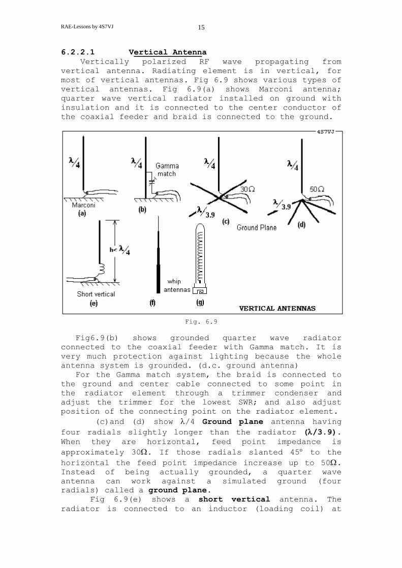
6.2.2.1 Vertical Antenna

Vertically polarized RF wave propagating from

vertical antenna. Radiating element is in vertical, for

most of vertical antennas. Fig 6.9 shows various types of

vertical antennas. Fig 6.9(a) shows Marconi antenna;

quarter wave vertical radiator installed on ground with

insulation and it is connected to the center conductor of

the coaxial feeder and braid is connected to the ground.

Fig. 6.9

Fig6.9(b) shows grounded quarter wave radiator

connected to the coaxial feeder with Gamma match. It is

very much protection against lighting because the whole

antenna system is grounded. (d.c. ground antenna)

For the Gamma match system, the braid is connected to

the ground and center cable connected to some point in

the radiator element through a trimmer condenser and

adjust the trimmer for the lowest SWR; and also adjust

position of the connecting point on the radiator element.

(c)and (d) show /4 Ground plane antenna having

four radials slightly longer than the radiator (/3.9).

When they are horizontal, feed point impedance is

approximately 30. If those radials slanted 45 to the

horizontal the feed point impedance increase up to 50. Instead of being actually grounded, a quarter wave

antenna can work against a simulated ground (four

radials) called a ground plane.

Fig 6.9(e) shows a short vertical antenna. The

radiator is connected to an inductor (loading coil) at


16

the bottom. This is very useful for low frequency bands

(40m or 80m); and also for mobile operations.

Fig 6.9(f) and (g) are Whip antennas. Fig 6.9(f) is a

telescopic type it is normally use for receivers (radio &

TV). Fig 6.9(g) is a rubber flex whip antenna; normally

use with hand held vhf TRX. The coiled antenna element is

covered by a insulated rubber cover.

6.2.2.2 Bi-Directional antenna

If any antenna radiates equally on opposite directions,

it is called as Bi-directional antenna. Following

antennas are Bi-directional

1. Long wire antenna

2. Dipole antenna

3. Loop antenna

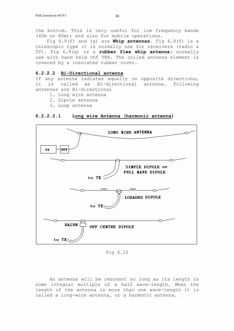
6.2.2.2.1 Long wire Antenna (harmonic antenna)

Fig 6.10

An antenna will be resonant so long as its length is

some integral multiple of a half wave-length. When the

length of the antenna is more than one wave-length it is

called a long-wire antenna, or a harmonic antenna.


17

This is not a good type of antenna because there are

considerable losses and antenna gain is low and SWR is

high. But very easy to install. Normally this type is

using with an ATU (antenna tuning unit) for reduce the

SWR, otherwise the final stage of the TX will be damage

by overheating. The efficiency of this antenna is very

low.

6.2.2.2.2 Dipole antenna

As mentioned earlier the dipole is the most simple

useful antenna which has two poles. The length of the

dipole is depend on the operating frequency or resonance

frequency of the dipole. There are several types of

dipoles as follows:

1. Simple dipole 2. Full wave dipole 3. Short dipole (loaded dipole) 4. Off center dipole

6.2.2.2.3 Simple dipole

If the length is equal to the electrical half-wave length

it is called as simple dipole or half wave dipole and it

is normally use as a reference antenna for antenna

experiments.

Approximate electrical ½ wave length = 0.95 x ½ x 300/f = 142/f meters

(f = frequency in MHz)

Theoretical Length = /2, (150/f meters). this is the

half wave length in free space for the particular

frequency. The actual length is shorter than the half

wave length. (due to velocity factor) It is depend on the

diameter of the wire, shorter length for higher

diameters.

6.2.2.2.4 Full-wave dipole

The length of this is a full wave length () or double

the size of the simple dipole.

6.2.2.2.5 Short dipole or Loaded Dipole

A short dipole is less than half the wave length. It

needs to be tuned to resonance by adding inductance

because of mismatch. It should be tuned for the lowest

SWR. This type is very much useful for a location having

limited space. The only disadvantage is the narrow

bandwidth. ^to download click here) www.qsl.net/4s7vj/download/Dipole.exe

http://www.qsl.net/4s7vj/download/Dipole.exe


18

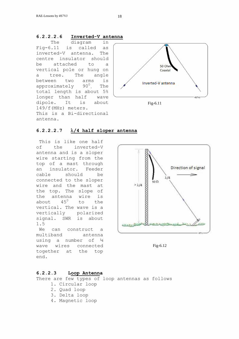
6.2.2.2.6 Inverted-V antenna

The diagram in

Fig-6.11 is called as

inverted-V antenna. The

centre insulator should

be attached to a

vertical pole or hung on

a tree. The angle

between two arms is

approximately 900. The

total length is about 5%

longer than half wave

dipole. It is about

149/f(MHz) meters.

This is a Bi-directional

antenna.

6.2.2.2.7 /4 half sloper antenna

This is like one half

of the inverted-V

antenna and is a sloper

wire starting from the

top of a mast through

an insulator. Feeder

cable should be

connected to the sloper

wire and the mast at

the top. The slope of

the antenna wire is

about 450 to the

vertical. The wave is a

vertically polarized

signal. SWR is about

1.5

We can construct a

multiband antenna

using a number of ¼

wave wires connected

together at the top

end.

6.2.2.3 Loop Antenna

There are few types of loop antennas as follows

1. Circular loop

2. Quad loop

3. Delta loop

4. Magnetic loop

Fig-6.11

Fig-6.12


19

Fig 6.13

6.2.2.3.1 Circular Loop Antenna

This is the most simple loop-antenna. A conductor

(tube) having a full wave length bend as a circle and two

ends connected to the feeder wire. Due to practical

difficulties this is suitable only, for vhf and uhf.

(Fig6.13-a)

6.2.2.3.2 Quad Loop

A conductor having a full wave length, bend as a

square and two ends connected to the feeder wire. (Fig

6.13-b) The total length of this antenna is 1.02 If it is attach with a gamma match system and adjusted

properly (SWR=1) it will be very much efficient broad

band antenna. (Fig 6.13-c)

6.2.2.3.3 Delta Loop

If the same Quad loop antenna bent as a triangle it is

called Delta-Loop antenna.(Fig 6.13-d)

6.2.2.3.4 Magnetic Loop antenna

The construction of this is appearing in the

diagram (Fig 6.13-e). An open loop constructed by a

copper wire or a copper tube, and both open ends at the

top are connected to a variable capacitor “C”. Inner

conductor of the coaxial cable connected at the point

“A”; braid is connected at the mid-point of the conductor

at the bottom. Position “A” is the deciding factor for

the characteristic impedance of the feeder.

The ideal small transmitting antenna would have

performance equal to a large antenna. This small loop-

antenna can approach that performance except for a

reduction in band-width. This is very narrow band, but

that effect can be overcome by re-tuning the capacitor


20

“C” for resonance. High voltage develop at the capacitor

(few kV). At the resonance SWR = 1. About one meter

diameter loop antenna can be use for whole HF band with

varying the capacitor. This capacitor is a high quality

high voltage type.

For more practical details click here

www.qsl.net/4s7vj/download/LoopAnt.exe

6.2.2.4 Directional or unidirectional antenna

It is possible to construct an antenna to radiate more

energy to one direction. It is called directional or

unidirectional antenna. Few directional antennas as

follows.

1. Cubical Quad antenna

2. Yagi antenna

3. Quagi antenna

4. Parabolic antenna

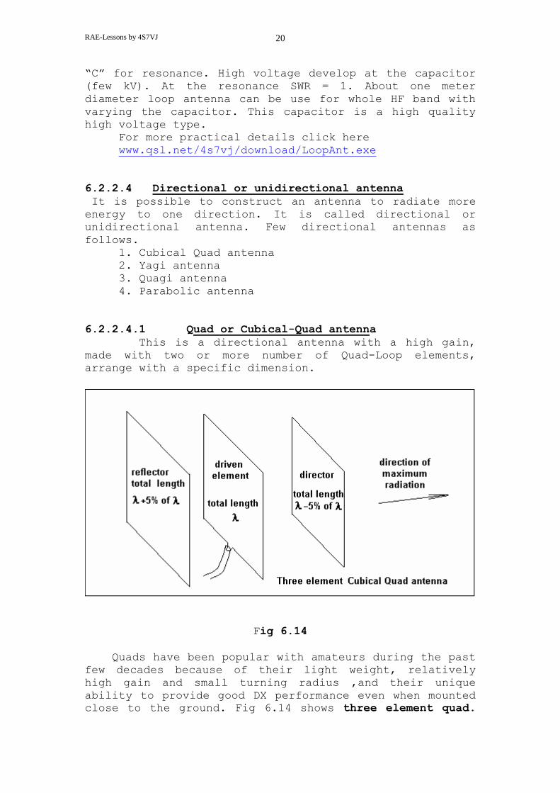
6.2.2.4.1 Quad or Cubical-Quad antenna

This is a directional antenna with a high gain,

made with two or more number of Quad-Loop elements,

arrange with a specific dimension.

Fig 6.14

Quads have been popular with amateurs during the past

few decades because of their light weight, relatively

high gain and small turning radius ,and their unique

ability to provide good DX performance even when mounted

close to the ground. Fig 6.14 shows three element quad.

http://www.qsl.net/4s7vj/download/LoopAnt.exe


21

The total length of the driven element is slightly more

than full wave length. Reflector is 5% greater than the

driven element and director is 5% smaller. All three

elements can be mount on an aluminum pipe called boom. If

the feeder wire connected through the Gamma-match system,

the performance is improving (SWR=1). The gain of a three

element Cubical Quad is about 9dB.

You can get full practical details from

http://www.qsl.net/4s7vj/download/My publication/Antenna Book.pdf

6.2.2.4.2 Yagi Antenna

This is a popular type of directional antenna. The

simplest Yagi antenna is one with just two elements as

indicated in Fig 6.15. Fig 6.15(a) has a reflector and a

driven element. The Fig-6.15(b) has a driven element and

a director. Fig 6.15(c) is a three element Yagi antenna

with a driven element (/2 long) a reflector (5% longer

than the driven element) and a director (5% shorter than

the driven element). The feeder line is connected to the

driven element. To improve the performance we must

install an impedance matching system in between the

driven element and the feeder wire. Fig 6.15(d) is a five

element Yagi antenna. If we increase the number of

elements according to the proper dimensions the

directional property gets increased. It means the antenna

gain for that particular direction gets increased.

Fig. 6.15

http://www.qsl.net/4s7vj/download/My%20publication/Antenna%20Book.pdf


22

Fig-6.16

We can use this gamma match system for any antenna

made out of aluminum tubes. The gamma capacitor made out

of a thin aluminum tube and insulated wire inserted into

the tube. For vary the capacitance we must vary the

length of wire inserted into the tube.

6.2.2.4.3 Quagi Antenna

This is a

combination of a Quad

and a Yagi. Normally

reflector and driven

element are like a

Cubical Quad and all

directors like Yagi.

6.2.2.4.4 Parabolic Antenna

This is a dipole antenna installed at the focal

point of a parabolic reflector. It is highly directional

and very high gain along the axis of the parabolic

reflector. This type called as micro wave antenna because

this type use only for frequencies higher than UHF.

(micro wave)

6.2.2.4.5 Receiving Antennas

Any type of antenna is possible to use with a

receiver; but if it is mismatch with the receiver, the

only problem is the strength of the input signal to the

RX become weak; there will be no damage or power loss

like transmitters. Most popular receiving antennas are

Fig-6.17


23

1. Ferrite rod antenna 2. Telescopic antenna 3. Loop antenna 4. Long wire antenna

6.2.2.5 Multi band Antennas

All antennas explained earlier work with a good

performance for one frequency. It is called the resonance

frequency. Some antennas work to a satisfactory level for

odd multiples of frequency. For Example 40m dipole can be

used for 15m.

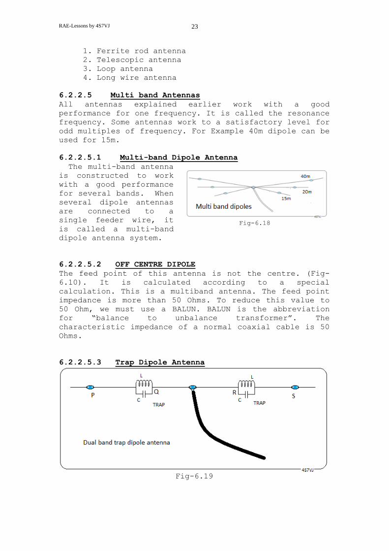
6.2.2.5.1 Multi-band Dipole Antenna

The multi-band antenna

is constructed to work

with a good performance

for several bands. When

several dipole antennas

are connected to a

single feeder wire, it

is called a multi-band

dipole antenna system.

6.2.2.5.2 OFF CENTRE DIPOLE

The feed point of this antenna is not the centre. (Fig-

6.10). It is calculated according to a special

calculation. This is a multiband antenna. The feed point

impedance is more than 50 Ohms. To reduce this value to

50 Ohm, we must use a BALUN. BALUN is the abbreviation

for “balance to unbalance transformer”. The

characteristic impedance of a normal coaxial cable is 50

Ohms.

6.2.2.5.3 Trap Dipole Antenna

Fig-6.19

Fig-6.18


24

Trap is a kind of RF filter constructed as a parallel

resonance circuit. Fig-6.19 has shown a two band trap

dipole antenna. If it is constructed for 14MHz and 7MHz

bands, traps should be tuned for 14MHz band. The 14MHz

signal is not passing through traps because the impedance

is maximum for 14MHz. Only QR portion is acting as 14MHz

antenna.

The total length is acting as 7MHz half wave dipole

antenna, because 7MHz signal is passing through traps.

The total length is little bit less than the 7MHz half

wave dipole because the wire length of the trap-coil also

to be counted.

We can construct a multi-band antenna for any number of

frequency bands.

6.2.2.5.4 Multi band Directional antenna

Fig-6.20

Fig-6.20 shows the most popular antenna among amateur

radio operators. It is a three element three band Yagi

constructed for 10m, 15m and 20m. There are 12 traps

connected as shown in the diagram. The trap is a parallel

LRC resonance circuit. There is no physical capacitor in

this trap. One side of the capacitor (C) is the external

aluminum tube and the other side is the coil (L).

6.2.2.6 Isotropic antenna

A simple way to appreciate the meaning of antenna gain is

to imagine the radiator to be totally enclosed in a

hollow sphere. If the radiation is distributed uniformly

over the interior surface of this sphere, the radiator is

said to be isotropic radiator or isotropic antenna.


25

An antenna which causes radiation to be concentrated into

any particular area of the surface of the sphere,

produces a greater intensity than that produced by an

isotropic antenna fed with equal power, is said to

exhibit a gain relative to an isotropic antenna.

The gain of an antenna is usually expressed as a power

ratio, either as a multiple of so many times or in

Decibel (dB) units. For example twice the power gain

could be represented as 3 dB. (3 = 10 Log2)

The gain of a simple half wave dipole is 2.15dB (or

2.15dBi)relative to an isotropic radiator. The expression

dBi is used to define the gain of an antenna system

relative to an isotropic radiator.

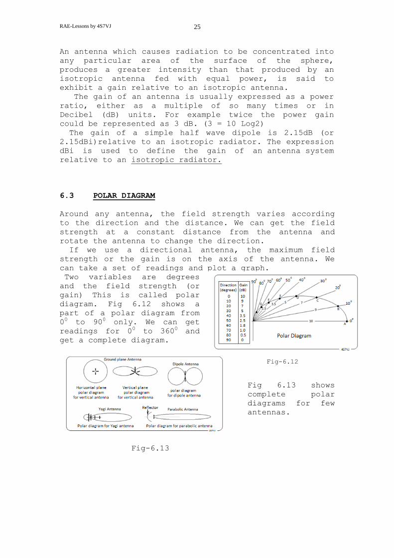
6.3 POLAR DIAGRAM

Around any antenna, the field strength varies according

to the direction and the distance. We can get the field

strength at a constant distance from the antenna and

rotate the antenna to change the direction.

If we use a directional antenna, the maximum field

strength or the gain is on the axis of the antenna. We

can take a set of readings and plot a graph.

Two variables are degrees

and the field strength (or

gain) This is called polar

diagram. Fig 6.12 shows a

part of a polar diagram from

00 to 90

0 only. We can get

readings for 00 to 360

0 and

get a complete diagram.

Fig 6.13 shows

complete polar

diagrams for few

antennas.

Fig-6.13

Fig-6.12

http://searchmobilecomputing.techtarget.com/definition/antenna

http://whatis.techtarget.com/definition/isotropic-radiator


26

6.4 WAVE PROAGATION

Radio wave is one portion of Electro Magnetic Waves.

Other portions are light waves, infra-red, ultra violet,

x-ray, gamma-ray etc. Straight line propagation is a

common property for all of these waves. Apart of that

refraction, reflection, diffraction and absorption also

exhibits. There are some properties varying with the

frequency. All types of electromagnetic waves are travel

with a constant speed. That is 300,000 km/s or 3x108 m/s in free space. In the air this is reduced very slightly

but it is negligible.

6.4.1 IONOSPHERIC PROPAGATION

Properties of the ionosphere

Regarding radio wave propagation through the

atmosphere and the ionosphere, there are three main

properties.

1. Absorption

2. Refraction

3. Reflection

Fig-6.14

6.4.1.1 ABSORPTION

In traveling through the ionosphere the wave gives

up some of its energy by setting the ionized particles

into motion. That means some percentage of the energy

belonging to the radio wave is lost or absorbed by the

ionosphere. This absorption is greater at lower

frequencies. It also increases with the intensity of

ionization, and with the density of the atmosphere in

the ionized region.


27

6.4.1.2 REFRACTION

When radio waves travel through the atmosphere, they

are bent slightly, due to variation of the density of

air layers and degree of ionization in the ionosphere.

Thus low-frequency waves are more readily bent than

those of high frequency. For this reason the lower

frequencies, 3.5 and 7 MHz are more reliable than the

higher frequencies. (14 to 28 MHz.) When the degree of

ionization is low value, the waves of the higher

frequencies are not bent enough to return to earth.

6.4.1.3. REFLECTION

When radio waves bend more and return to earth, it

is call reflection. This reflection happens from upper

layer of the ionosphere. These layers are named D, E,

and F (F1, F2). (Fig-6.15)

Fig-6.15

Classification and Definitions of the Ionosphere

6.4.1.3.1 D-LAYER

In the daytime there is a still lower ionized area,

the D region. D region ionization is proportional to

the angle of elevation of the Sun and is greatest at

noon. The lower frequencies (1.8 and 3.5 MHz) are almost

completely absorbed by this layer, and only the high-

angle radiation penetrates and is reflected by the E

layer.

6.4.1.3.2 E-LAYER

This is the lowest useful ionized layer, and the

average height is about 120km. The E- layer normally

disappears after Sunset.


28

6.4.1.3.3 F-LAYER

This is the most important layer, which has a height

of about 280km at night. In the daytime the F layer

splits into two parts, the F1 and F2 layers,(Fig-6.15)

with average virtual heights of 220km and 320km

respectively. These layers merge again at sunset into

the F layer. (280km)

Fig-6.16

6.4.2 ANGLE OF RADIATION

The angle between the direction of the wave and

the horizon or tangent of the earth is called the wave

angle or angle of radiation. This is denoted by Ø in the

diagram of Fig-6.16

6.4.3 GROUND WAVE

The horizontal waves from the TX antenna (W1 in the

Fig 1.10)travels a line of sight distance or little more,

parallel to the ground. This is called ground wave.

6.4.4 CRITICAL ANGLE

The wave at a somewhat lower angle is just capable of

being returned by the ionosphere. (W2 in the Fig 1.10)

This radiation angle is called the critical angle.(Ø in

the Fig-6.16)

Radiation at angles more than the critical angle do

not return to Earth, because it is only slightly bent in

the ionosphere and to pass through it. This is called

sky wave.The radiation at angles smaller than the


29

critical angle return to the Earth at a long distance.

(W3 in Fig-6.16)

6.4.5 SKIP DISTANCE and SKIP ZONE

When the wave angle is equal to the critical angle for

a particular frequency and for a particular time for the

day, it is reflect and return to the Earth at a certain

distance. (at R2 in Fig 1.10) For lower angle of radiation

signals are reach beyond that point.(at R3 in Fig 1.10)

This is illustrated in Fig-1.10, where Ø and smaller

radiation angles give useful signals while waves sent at

higher angles penetrate the layer and are not returned.

The distance between T and R2 is therefore the shortest

possible distance at the particular frequency, and for a

particular time for the day, over which communicate by

ionospheric reflection can be accomplished. This distance

is called skip distance.

The area between the end of the useful ground wave

and the beginning of the ionospheric wave reception is

called the skip zone.

The extent of the skip zone depends upon the

frequency and the state of the ionosphere, and also upon

the height of the layer in which the reflection takes

place.

6.4.6 CRITICAL FREQUENCY

If the frequency is low enough, a wave sent vertically

to the ionosphere will be reflected back down to the

transmitting point. (Eg: 80 m-band with horizontal

Quad loop). If the frequency is then gradually

increased, eventually a frequency will be reached

where this vertical reflection just fails to occur.

This is the critical frequency for the layer under

consideration. When the operating frequency is

below the critical frequency, there is no SKIP ZONE.

The critical frequency is a useful index to the

highest frequency that can be used to transmit over a

specified distance.

6.4.7 MAXIMUM USABLE FREQUENCY (MUF)

If a radio wave leaving the transmitting point 'T' and

receive at the point 'R', for example, at a frequency

14 MHz., and if a higher frequency would skip over

the receiving point, then 14 MHz. is the m.u.f. for

the distance between T and R. The greatest possible

distance is covered when the wave leaves along the

tangent to the earth, that means horizontal. (Zero wave

angle) Under average conditions, this distance is about

4000 km., for the F2 layer, and 2000 km., for the E

layer. This distance varies depending on the height of

the layer. Frequencies above the m.u.f. do not return to


30

earth at any distance. The 4000km m.u.f. for the F2

layer is approximately three times the critical frequency

for that layer. For the E layer the 2000 km m.u.f. is

about 5 times the critical frequency.

6.4.8 LOWEST USABLE FREQUENCY (LUF)

There is a lower limit to the band of frequencies

which can be selected for a particular application. This

is set by the lowest usable frequency, below which the

circuit becomes either unworkable or uneconomical because

of the effects of absorption and the level of radio

noise.

6.5 SUN-SPOT CYCLE

The propagation of the HF radio wave depends on the

11 year Sunspot cycle Activity. The maximum sunspot

season is the best for HF Communication. (Eg:- 1980 &

1991, next 2002) The critical frequencies are highest

During sunspot maximum period. During the period of

minimum sunspot activity, the lower frequencies (40m &

80m) are the only usable bands at night.

6.5.1 PROPAGATION IN THE HF BANDS

6.5.1.1 160m-band (1.8-2.0 MHz)

160m band offers reliable working over range up to

40 km during daytime. On winter nights ranges up to

several thousand km.

6.5.1.2 80m-band (3.5-3.8 MHz)

During the day time 80m-band covers upto about 300

km. This band is more useful during the night because the

range is several thousand miles. Transoceanic contacts

are regularly made during the winter months. During

the summer the static level is high.

6.5.1.3 40m-band (7.0-7.1 MHz)

40m-band has many of the characteristics as 80m-band

except that the distance, that can be covered during the

day and night hours are increased. Day-light distance

upto about thousand miles and during winter nights it is

possible to work stations as far as the other side of the

world. The signals following the darkness path. Summer

static is much less of a problem than on 80m.

6.5.1.4 30m-band (10.1 – 10.15 MHz)

This is a WARC band introduced in 1980, permitted

only for CW operation . This band is usable during 24

hours of the day. This is usable for 1500 to 2000km

during the day time and throughout the world during

night.


31

6.5.1.5 20m-band (14.0-14.35 MHz)

This is the best amateur band for DX work. During the

high portion of the sunspot cycle it is open to some part

of the world practically throughout the 24 hours,

while during a sunspot minimum it is generally useful

only during twilight hours and the dawn and dusk periods.

There is practically always a skip zone on the band.

6.5.1.6 17m-band (18.068 – 18.168 MHz)

This is a WARC band introduced in 1980. Most of the

properties of this band are like the 15m band. It is more

reliable during day-time and early evenings. Normally

this band gets weaker and weaker after sunset. During

minimum sunspot period, this band is fairly active only

around noon even though it is only for equatorial

regions.

6.5.1.7 15m-band (21.0-21.45 MHz)

15m-band shows highly variable characteristics

depending on the sunspot cycle. During sunspot maximum it

is useful for long distance work during a large part of

the 24 hours, but in years of low sunspot activity it

is almost wholly a daytime band, and sometimes unusable

even in daytime. However, it is often possible

to use it for distances up to 1500 miles or more.

6.5.1.8 12m-band (24.890-24.990 MHz)

This is a WARC band introduced in 1980. This band has

combined properties of 10m and 15m bands. This is limited

to day time during sunspots minimum and average seasons.

This is a good DX band after sunset during sunspot

maximum periods.

6.5.1.9 10m-band (28.0-29.7 MHz)

10m-band is generally considered to be a DX-band during

the daylight hours (except in summer) and good for local

work during the hours of darkness, for about half the

sunspot cycle. At the sunspot minimum the band is usually

dead.

6.5.1.10 6m-band (50.0-50.4 MHz)

This is the lowest frequency band in vhf range. For

this band noise and interference are minimum. Normally

this 6m-band is suitable for short distance communication

up to about 150 km, but occasionally having ionospheric

reflection. This is suitable for DXing due to the

reflection by F2 layer during sunspot maximum season.

6.5.1.11 WARC bands

International Amateur Radio Union (IARU)is the

international organization of the amateur radio service.


32

International Telecommunication Union (ITU) is the

international organization for all communication systems

in the world. In 1979 there was a conference of the above

organizations called WARC (World Administrative Radio

Conference). At this conference it was decided to give

another three new bands for the amateur radio service

called WARC-bands. They are as follows:

30m – 10.100 – 10.150 MHz (CW only)

17m – 18.068 – 18.168 MHz

12m – 24.890 – 24.990 MHz

radio amateur exam - qsl.net · radio amateur exam general class by 4s7vj chapter-6 transmission...

Documents