radiomics in pet imaging: a practical guide for newcomers
TRANSCRIPT

HAL Id: hal-03320546https://hal.archives-ouvertes.fr/hal-03320546
Submitted on 16 Aug 2021
HAL is a multi-disciplinary open accessarchive for the deposit and dissemination of sci-entific research documents, whether they are pub-lished or not. The documents may come fromteaching and research institutions in France orabroad, or from public or private research centers.
L’archive ouverte pluridisciplinaire HAL, estdestinée au dépôt et à la diffusion de documentsscientifiques de niveau recherche, publiés ou non,émanant des établissements d’enseignement et derecherche français ou étrangers, des laboratoirespublics ou privés.
Radiomics in PET imaging: a practical guide fornewcomers
Fanny Orlhac, Christophe Nioche, Ivan Klyuzhin, Arman Rahmim, IrèneBuvat
To cite this version:Fanny Orlhac, Christophe Nioche, Ivan Klyuzhin, Arman Rahmim, Irène Buvat. Radiomics in PETimaging: a practical guide for newcomers. PET Clinics, WB Saunders, In press. �hal-03320546�

Radiomics in PET imaging: a practical guide for newcomers
Fanny Orlhac* (PhD)1, Christophe Nioche (PhD)1, Ivan Klyuzhin (PhD)2,3,
Arman Rahmim (PhD)2,3, Irène Buvat (PhD)1
1: Institut Curie, Université PSL, Inserm, U1288 LITO, Orsay France.
2: Department of Integrative Oncology, BC Cancer Research Institute, Vancouver, BC, Canada.
3: Department of Radiology, University of British Columbia, Vancouver, BC, Canada.
* Corresponding author: Fanny Orlhac ([email protected])
Laboratoire d’Imagerie Translationnelle en Oncologie (LITO)
U1288 Université Paris Saclay/Inserm/Institut Curie
Institut Curie Centre De Recherche, Centre Universitaire
Bâtiment 101B, Rue Henri Becquerel, CS 90030
91401 ORSAY Cedex, FRANCE
Synopsis
Radiomics has undergone considerable development in recent years. In PET imaging, very promising
results concerning the ability of handcrafted features to predict the biological characteristics of lesions
and to assess patient prognosis or response to treatment have been reported in the literature. This
article presents a checklist for designing a reliable radiomic study, gives an overview of the steps of the
pipeline, and outlines approaches for data harmonization. Tips are provided for critical reading of the
content of articles. The advantages and limitations of handcrafted radiomics compared to deep
learning approaches for the characterization of PET images are also discussed.
Keywords (3-8): Radiomics, PET, texture, heterogeneity, harmonization
Key points (3-5):
In the literature, promising results report links between the radiomic feature values
measured on PET images and the biological characteristics of lesions, patient prognosis and
response to treatments.
Each step in the radiomic analysis pipeline influences the feature values and should be
carefully reported to allow other teams to reproduce the findings.
Harmonization methods will play a key role in the development of radiomic models using
heterogeneous data and in their deployment for multicenter validation.
Deep learning methods can be used to extract new features and could bring a new and
complementary perspective to current engineered features.
Technical terms:
1. Artificial Intelligence
2. Biomarker
3. Cohort
4. Dataset
5. Deep learning
6. Discretization
7. Feature
8. Handcrafted
9. Harmonization
10. Heterogeneity
11. Histogram
12. Medical images
13. Model
14. Multicenter
15. PET
16. Quantification
17. Radiomics
18. Shape
19. Texture
20. Validation

Must read:
Gillies RJ, Kinahan PE, Hricak H. Radiomics: images are more than pictures, they are data. Radiology.
2016;278:563-577.
Reuzé S, Schernberg A, Orlhac F, et al. Radiomics in nuclear medicine applied to radiation therapy:
methods, pitfalls, and challenges. Int J Radiat Oncol Biol Phys. 2018;102:1117-1142.
Zwanenburg A. Radiomics in nuclear medicine: robustness, reproducibility, standardization, and how
to avoid data analysis traps and replication crisis. Eur J Nucl Med Mol Imaging. 2019;46:2638-2655.
Nice to read:
Buvat I, Orlhac F. The dark side of radiomics: on the paramount importance of publishing negative results. J Nucl Med. 2019;60:1543-1544.
Mayerhoefer ME, Materka A, Langs G, et al. Introduction to radiomics. J Nucl Med. 2020;61:488-495.
Orlhac F, Boughdad S, Philippe C, et al. A postreconstruction harmonization method for multicenter
radiomic studies in PET. J Nucl Med. 2018;59:1321-1328.
Papp L, Spielvogel CP, Rausch I, Hacker M, Beyer T. Personalizing medicine through hybrid imaging and medical big data analysis. Front Phys. 2018;6.
Zwanenburg A, Vallières M, Abdalah MA, et al. The Image Biomarker Standardization Initiative:
standardized quantitative radiomics for high-throughput image-based phenotyping. Radiology.
2020;295:328-338.

Introduction
The term “radiomics” was first introduced in 2010 by Gillies et al.1 and was later defined as “the
conversion of digital images into mineable high-dimensional data”2. The analysis of these high-
dimensional data is intended to provide information on the biological characteristics of tumors, patient
prognosis or the response to treatments. These data can reflect the signal intensity distribution,
texture or shape of the signal in a given volume of interest (VOI) in the image. Although the term
"radiomics" is relatively new, many studies have reported on advanced image analysis in the past and
investigated the relationship between sophisticated measurements and biological characteristics. For
instance, even before the 2000s, authors were studying the relationship between fractal analysis and
striatal dopamine uptake3 and the use of a co-occurrence matrix to classify lung nodules4. Since 2007,
the Quantitative Imaging Biomarkers Alliance (QIBA) working groups have also published
recommendations "to advance quantitative imaging and the use of imaging biomarkers in clinical trials
and clinical practice"5. Among the 2,970 papers associated with the keyword "radiomics" on PubMed
(between 2012-01 and 2020-12), 424 mention PET imaging (Figure 1). These articles mainly concern
oncologic applications regarding the lungs (30%), the head and neck (16%), the esophagus (7%), breast
cancer (6%) and lymphoma (6%). In these articles, the authors investigated the relationship between
radiomic feature values and the biological characteristics of the lesions (39%), patient prognosis (27%)
or the response to treatments (24%). In these papers, features were mainly extracted from PET images
obtained after injection of 18F-fluorodeoxyglucose (18F-FDG, 87%) but also using other radiotracers
such as 18F-fluoroethyl-L-tyrosine (18F-FET, 2%), 11C-methionine (11C-MET, 2%) and 68Ga-prostate-
specific membrane antigen (68Ga-PSMA, 2%). A small proportion of articles (10%) report
methodological contributions regarding the impact of acquisition and reconstruction parameters of
PET images and of the different steps of the radiomic analysis pipeline on feature values based on
phantom and/or clinical data.
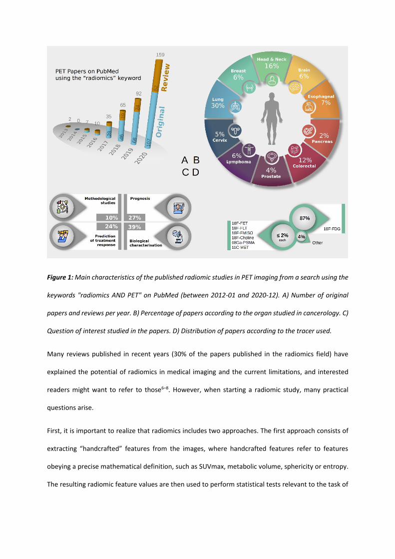
Figure 1: Main characteristics of the published radiomic studies in PET imaging from a search using the
keywords "radiomics AND PET" on PubMed (between 2012-01 and 2020-12). A) Number of original
papers and reviews per year. B) Percentage of papers according to the organ studied in cancerology. C)
Question of interest studied in the papers. D) Distribution of papers according to the tracer used.
Many reviews published in recent years (30% of the papers published in the radiomics field) have
explained the potential of radiomics in medical imaging and the current limitations, and interested
readers might want to refer to those6–8. However, when starting a radiomic study, many practical
questions arise.
First, it is important to realize that radiomics includes two approaches. The first approach consists of
extracting “handcrafted” features from the images, where handcrafted features refer to features
obeying a precise mathematical definition, such as SUVmax, metabolic volume, sphericity or entropy.
The resulting radiomic feature values are then used to perform statistical tests relevant to the task of

interest or as an input for a multivariate classifier, most often designed using a machine learning
approach, such as the logistic regression, support vector machine, or random forest.
A second approach consists of using images or image VOIs directly as input to a neural network, such
as a convolutional neural network (CNN), to obtain a classification or a prediction. This approach can
be called deep radiomics as it still treats the images as high-dimensional mineable data (each voxel is
an input variable); however, the radiomic features are no longer predefined when using handcrafted
features but are learned by the CNN itself as a function of the input images and of the task.
Deep radiomics can also consist of extracting "deep" features using a CNN and then providing these
features to a classifier 9,10. Alternatively, deep radiomics first involves the calculation of radiomic
parametric images using the definition of handcrafted features and then inputs these maps into a deep
neural network. In short, deep radiomics will be used thereafter anytime a deep neural network is used
in a certain step of the radiomic pipeline.
The difficulty for physicians to precisely quantify heterogeneity, the lack of intra- and interobserver
reproducibility, and the challenge of coanalyzing many pieces of information at the same time are all
arguments in favor of radiomics. Several studies have proven that radiomic indices can quantify the
heterogeneity perceived by physicians11,12 and that the macroscopic phenotypes measured from
images are related to the density and spatial organization of cells at the microscopic scale13–15. Despite
the indisputable potential of radiomics in PET, no model has yet proven its superiority over existing
methods based on common features (e.g., SUVmax or metabolic volume) in multicenter and
multicohort settings and by different independent investigators. To produce sound radiomic models
amenable to clinical translation, a thorough understanding of the impact of the choices made in each
step of a radiomic study is absolutely necessary.
Therefore, the main objective of this paper is to offer a practical guide to help interested readers
establish a radiomic study involving PET images and "handcrafted" features. In addition, we discuss

key aspects to consider when analyzing the literature in this field. Finally, we explain how deep
radiomics can complement handcrafted radiomics.
Checklist to design a reliable radiomic study
Before initiating a radiomic study, a number of questions should be considered to determine if the
study is relevant and feasible. Here, we list the major points to be examined (Figure 2).
Figure 2: A) Checklist for a reliable radiomic study. B) Sham test: comparison of the performances using
real labels and randomly assigned labels to test the significance of findings.

1) Identify a relevant question
As with any scientific study, the question of interest will determine the impact of the investigation.
From a clinical point of view, the question of interest may relate to patient management (for instance,
the prediction of patient response or survival) or to a better understanding of a disease (for instance,
the distinction between different molecular subtypes from phenotypic data). The level of performance
that would make the radiomic approach appealing compared to state-of-the-art approaches should be
indicated or, alternatively, the reason why a radiomic approach would be desirable. From a physics
point of view, the goal might be to better understand radiomics or the factors that can influence
feature values and/or to propose corrections or improvements for enhanced radiomic models. The
relevance of the question and the contribution of the investigation should be carefully inspected based
on a bibliographic search.
2) Review the state-of-the-art
In radiomics, there is at least as much value in confirming a previously published result as in
establishing a new model16. As obvious as this may seem, the first instinct should be to review the
existing literature on the subject of interest to determine whether the question has already been
addressed by others and how. In particular, it is useful to know if a clinical question has already been
investigated using conventional features (for instance, SUVmax, metabolic volume, and total lesion
glycolysis) and which added value is expected from the use of more sophisticated radiomic features. If
a clinical question has already been dealt with using radiomics, the first step could be to try to
reproduce the findings. Indeed, at the moment, although hundreds of radiomic models are published,
publications that independently validate radiomic models published by others are scarce, if they even
exist16. This lack of reproducible results is certainly the greatest bottleneck for advancing the field, and
it is an essential prerequisite for clinical translation.

3) Collect data
Once the question of interest has been identified and well defined, the availability of the data needed
to conduct the study with the expected statistical power should be checked. Needless to say, the data
should comply with the legislation regarding data privacy (for instance, it should be GDPR-compliant
in Europe). When collecting the data, the inclusion/exclusion criteria should be precisely defined and
later clearly reported in any publication. In the vast majority of cases, images alone are insufficient;
and additional data has, such as that on age, sex, cancer subtype, comedication, and treatment, have
to be accessible and collected as these factors can influence the measurements made from the images.
For example, the age of patients can influence the radiomic feature values measured in breast cancer
lesions17 and thus be a confounding factor. For supervised learning, a ground truth or surrogate ground
truth must be available and can be based on histological analysis (e.g., subtype and the presence of
mutations), radiological evaluation (e.g., response to treatment evaluated via RECIST) or follow-up
(e.g., recurrence, progression-free survival, and overall survival). In practice, this ground truth might
be imperfect, especially when it is derived from a physician’s diagnosis, and this might influence the
performance of the model and its generalization.
The quantity of images needed for a specific investigation does not obey a simple rule. It depends on
the difficulty of the task, the complexity of the mathematical model and the approaches used
(handcrafted or deep radiomics). If the biological signal is weak or the data have high heterogeneity,
several hundred or even thousand patients may be needed. If the biological signal is well reflected by
the radiomic features, fewer than 100 patients might be sufficient to build and validate a handcrafted
radiomic model using cross-validation18. Moreover, the required number of images may grow when
several hundred radiomic features are investigated to account for an increased false discovery rate. A
downsampling strategy can be used to obtain some insights into how the performance evolves as a
function of the number of patients and the number of patients needed to achieve a given
performance19. Overall, as the definition of handcrafted features is fixed, a smaller number of patients
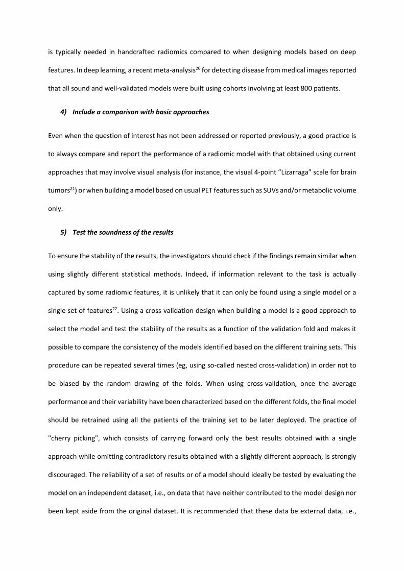
is typically needed in handcrafted radiomics compared to when designing models based on deep
features. In deep learning, a recent meta-analysis20 for detecting disease from medical images reported
that all sound and well-validated models were built using cohorts involving at least 800 patients.
4) Include a comparison with basic approaches
Even when the question of interest has not been addressed or reported previously, a good practice is
to always compare and report the performance of a radiomic model with that obtained using current
approaches that may involve visual analysis (for instance, the visual 4-point “Lizarraga” scale for brain
tumors21) or when building a model based on usual PET features such as SUVs and/or metabolic volume
only.
5) Test the soundness of the results
To ensure the stability of the results, the investigators should check if the findings remain similar when
using slightly different statistical methods. Indeed, if information relevant to the task is actually
captured by some radiomic features, it is unlikely that it can only be found using a single model or a
single set of features22. Using a cross-validation design when building a model is a good approach to
select the model and test the stability of the results as a function of the validation fold and makes it
possible to compare the consistency of the models identified based on the different training sets. This
procedure can be repeated several times (eg, using so-called nested cross-validation) in order not to
be biased by the random drawing of the folds. When using cross-validation, once the average
performance and their variability have been characterized based on the different folds, the final model
should be retrained using all the patients of the training set to be later deployed. The practice of
"cherry picking", which consists of carrying forward only the best results obtained with a single
approach while omitting contradictory results obtained with a slightly different approach, is strongly
discouraged. The reliability of a set of results or of a model should ideally be tested by evaluating the
model on an independent dataset, i.e., on data that have neither contributed to the model design nor
been kept aside from the original dataset. It is recommended that these data be external data, i.e.,
acquired on a different device or from a different center to validate the performance in slightly
different conditions, to better demonstrate the validity of the findings. Another useful evaluation
approach is to test the extensive model building or data analysis pipeline using sham data19. This
involves randomly assigning the real labels to the actual data and comparing the performance with
that obtained when the labels are correctly assigned. For this approach to be informative, the complete
analysis process should be applied to the sham data (including the feature selection process, if any),
and several sham datasets (corresponding to several random drawings) should be used so that the
statistical distribution of the relevant figures of merit can be determined in sham conditions. The
figures of merit measured on the real data can then be compared to those statistical distributions to
establish the significance of the results (Figure 2). Other approaches such as image simulations11,23 can
be used to check the robustness of the results and/or the interpretation of features.
The use of a hypothesis-driven approach can help to minimize false discovery. For example, this is the
case when a new feature is designed to quantify a characteristic perceived by physicians as predictive
or prognostic (for instance, the quantification of the presence of severity of a necrosis in a tumor). The
investigation of the biological plausibility of a radiomic model by deciphering the information reflected
by the different features and the associated weights improves the confidence in the results. The use
of unsupervised feature selection methods, test-retests, or studies investigating the influence of
segmentation methods can eliminate irrelevant or insufficiently robust variables and thus reduce false
discoveries.
6) Publish and share
A scientific study should be replicable, and its impact will actually depend on the ability of independent
researchers to confirm the findings. To make that possible, the steps used to produce the results
should be precisely described (see below), and the images (or extracted radiomic feature values)
and/or the algorithm could be shared whenever possible. If the source code does not have to be
shared, an executable or information regarding how to access a prototype implementing the model

can be sufficient. This allows colleagues to challenge and hopefully confirm the results on the same
data or test the classification or prediction model independently on other data. The huge importance
of data sharing was recently well illustrated by Welch et al.23 who were able to demonstrate the
spurious interpretation of a previously published prognostic signature through an independent
reanalysis of the data provided by the authors.
Sharing the data and methods should prompt the investigators to clearly define the limitations of their
findings, including the description of the situations in which they expect their model to fail or
conclusions not to be true. Reporting negative results is essential to avoid the misuse of algorithms or
excessive generalization of results16.
How to read an article reporting a radiomics study
As in any scientific discipline, reading an article in the radiomics field calls for the reader's critical sense.
The Materials & Methods section is as important as if not more important than the results and
scrutinization of the supplemental data is often needed to avoid misinterpretation. The reader should
in particular pay attention to whether the data are homogeneous (well defined patient cohort, same
acquisition protocol for all patients, same treatment, etc.) and, if not, to the strategy implemented to
rule out or account for possible confounding factors caused by that heterogeneity. The validation
approach used in the paper should be examined carefully to determine whether the corresponding
results support the claim. The positioning of the results with respect to clinical practice or previous
work addressing the same topic should be reported so that the findings are put into perspective. Last,
whether the conclusion can be checked by others will actually determine the impact of the findings.
Recently, a Radiomic Quality Score (RQS) has been proposed to assess the quality of radiomic studies24.
This score, including 16 criteria related to the acquisition protocol up to data sharing, is provided in
order to “both reward and penalize the methodology and analyses of a study, consequently
encouraging the best scientific practice”24 according to the authors. However, this score does not
necessarily reflect the reliability of the results and of their interpretation. Indeed, the study by Aerts
et al.25 had a score of 55.6% according to 26, which is higher than all other papers mentioned in this
article (range: [0-50%]). However, it was still highly biased, including a spurious interpretation of the
findings23. Other checklists not specifically dedicated to radiomic studies, such as Transparent
Reporting of a multivariable prediction model for Individual Prognosis Or Diagnosis (TRIPOD)27 and
Checklist for Artificial Intelligence in Medical Imaging (CLAIM)28 for example, can also be considered
when conducting radiomic studies, as they include good practice rules that are also very relevant to
radiomic studies.
Therefore, the best way to judge the quality of a radiomic study is to become familiar with the various
steps of the pipeline and to understand their influences on the results. We thus explain these different
steps hereafter.
Handcrafted radiomics
A handcrafted radiomics pipeline can be described using five steps. The investigator builds a database
of medical images, and VOIs are defined. This is followed by a spatial resampling step and an intensity
discretization step (except for shape features) before the calculation of radiomic features (Figure 2).
As many different practices have been reported in the literature29, an international consortium named
the Image Biomarker Standardization Initiative (IBSI) involving 25 teams30 has been established to
precisely define the different options for each step and provide benchmark data to check that different
radiomic software programs provide the same value for specific well-defined features. This
standardization step remains a fundamental prerequisite to ensure that the calculated radiomic values
follow a reference standard that others can replicate. The IBSI has produced a reference guide31 with
definitions of features and has listed most options for the preprocessing steps. Reference to this guide
is then extremely useful to explain how a specific step (e.g., interpolation) in the radiomic feature
calculation process is performed. However, based on this guide, it may be difficult to choose the
optimal setting among all the available options since it depends on the type of medical images that are
analyzed, the device used, the imaging protocol, the type of cancer, and the question of interest. Many
methodological choices remain the responsibility of the investigator. Based on our experience and the
data from the literature, here we present some guidelines to perform radiomic analysis in PET.
Segmentation
There is no consensus regarding how the structure of interest should be segmented before subsequent
radiomic analysis 32,33. However, it has been widely demonstrated that radiomic features are sensitive
to the segmentation method used34–38, with an intraclass correlation coefficient that can vary from 0.0
to 1 depending on the segmentation methods and the radiomic features. For the sake of
reproducibility, it therefore seems preferable to use an automatic or semiautomatic method rather
than manual segmentation. In addition, the impact that the segmentation method has on the radiomic
model performance should be systematically analyzed, unless the radiomic features involved in the
models have already been demonstrated not to be sensitive to the region delineation (eg, SUVmax).
In tumor imaging, the primary tumor is usually segmented, and radiomic analysis is performed using
this single VOI. However, extending the radiomic analysis to the peritumoral area (sometimes called
ring) at the interface between the lesion and the surrounding healthy tissue39 to possibly capture
relevant information related to the tumor environment has been proposed. When multiple tumor sites
are present, there are no rules as to how to combine the radiomic features measured in different
lesions, and specific features reflecting the distribution of lesions can then be extracted 40,41.
In cancer patients, there is an increasing interest in studying metabolism and its heterogeneity in
“healthy” organs, especially lymphoid organs, to determine whether such features might actually
provide valuable information to prognostic or predictive models. This is often performed by locating a
small volume of a fixed size (on the order of a few ml) in the organ of interest, such as the liver, spleen,
bone marrow or adipose tissue, to derive radiomic features42.
To reduce the variability in radiomic feature values due to the VOI definition, the rule of thumb is to
use the same strategy for all patients in the cohort (e.g., the same threshold corresponding to 40% of
SUVmax or the anatomical contour based on CT or MR images). When this is not possible, the influence
of the difference in VOI delineation should be considered in the analysis of the results. For biological
characterization (e.g., to distinguish between tumor subtypes), focusing on the tumor VOI may be
sufficient. Conversely, if the objective is to predict the response to treatments (especially in the case
of immunotherapy) or the survival of the patients, considering radiomic features measured in organs
other than the tumors might be useful43.
Spatial resampling
For example, when the algorithm uses neighboring voxel values to compute a texture feature, it is
implicitly assumed that the voxels are isotropic, that is, that all the neighbors of a voxel are located at
the same distance in the three directions. Spatial resampling is thus needed when this is not the case.
This makes the extraction of textural features rotationally invariant. In addition, the size of the voxels
strongly influences the values of some features44,45. Therefore, feature values should be compared only
if they are calculated from images with the same voxel size. Spatial resampling involves interpolation,
such as nearest neighbor, trilinear, tricubic convolution, and tricubic spline interpolation; and the
choice of the method influences the feature values46. For this resampling step, there is no single best
option. For instance, if the voxel size in the original image is 1x1x3 mm3, it is possible to resample them
to 1x1x1 mm3, 2x2x2 mm3 or 3x3x3 mm3, but it would not make sense to resample to 0.1 or 10 mm.
The rule of thumb is to choose the same isotropic voxel size with the same interpolation method for
all patients in the cohort. After a resampling strategy is used and a successful model is validated, it is
always recommended that whether the model performance is highly dependent on the resampling
settings be checked.
Intensity discretization
Intensity discretization is a mandatory step to calculate some radiomic features in order to group close
gray levels together to reduce the impact of noise. In the literature, two techniques are mostly used:
relative discretization, corresponding to setting the number of gray levels or bins; and absolute
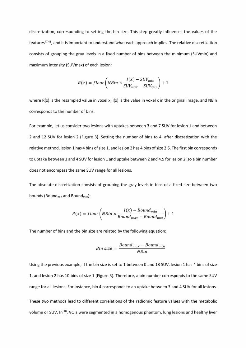
discretization, corresponding to setting the bin size. This step greatly influences the values of the
features47,48, and it is important to understand what each approach implies. The relative discretization
consists of grouping the gray levels in a fixed number of bins between the minimum (SUVmin) and
maximum intensity (SUVmax) of each lesion:
𝑅(𝑥) = 𝑓𝑙𝑜𝑜𝑟 (𝑁𝐵𝑖𝑛 ×𝐼(𝑥) − 𝑆𝑈𝑉𝑚𝑖𝑛
𝑆𝑈𝑉𝑚𝑎𝑥 − 𝑆𝑈𝑉𝑚𝑖𝑛) + 1
where R(x) is the resampled value in voxel x, I(x) is the value in voxel x in the original image, and NBin
corresponds to the number of bins.
For example, let us consider two lesions with uptakes between 3 and 7 SUV for lesion 1 and between
2 and 12 SUV for lesion 2 (Figure 3). Setting the number of bins to 4, after discretization with the
relative method, lesion 1 has 4 bins of size 1, and lesion 2 has 4 bins of size 2.5. The first bin corresponds
to uptake between 3 and 4 SUV for lesion 1 and uptake between 2 and 4.5 for lesion 2, so a bin number
does not encompass the same SUV range for all lesions.
The absolute discretization consists of grouping the gray levels in bins of a fixed size between two
bounds (Boundmin and Boundmax):
𝑅(𝑥) = 𝑓𝑙𝑜𝑜𝑟 (𝑁𝐵𝑖𝑛 ×𝐼(𝑥) − 𝐵𝑜𝑢𝑛𝑑𝑚𝑖𝑛
𝐵𝑜𝑢𝑛𝑑𝑚𝑎𝑥 − 𝐵𝑜𝑢𝑛𝑑𝑚𝑖𝑛) + 1
The number of bins and the bin size are related by the following equation:
𝐵𝑖𝑛 𝑠𝑖𝑧𝑒 = 𝐵𝑜𝑢𝑛𝑑𝑚𝑎𝑥 − 𝐵𝑜𝑢𝑛𝑑𝑚𝑖𝑛
𝑁𝐵𝑖𝑛
Using the previous example, if the bin size is set to 1 between 0 and 13 SUV, lesion 1 has 4 bins of size
1, and lesion 2 has 10 bins of size 1 (Figure 3). Therefore, a bin number corresponds to the same SUV
range for all lesions. For instance, bin 4 corresponds to an uptake between 3 and 4 SUV for all lesions.
These two methods lead to different correlations of the radiomic feature values with the metabolic
volume or SUV. In 48, VOIs were segmented in a homogenous phantom, lung lesions and healthy liver

tissue. With relative discretization, the entropy values are highly correlated with metabolic volume
and are not different between the three regions (phantom, lung lesion and liver region), whereas
visually, the heterogeneity is quite different. With absolute discretization, the entropy values are
different between the three regions (with higher values for the tumor than for the liver tissue and
higher values in the liver compared to the phantom), and the features are much less dependent on the
volume but are more correlated with SUVs. As seen from this example, in PET, features calculated
using absolute discretization thus better reflect visual impression. The choice of the bin size influences
the results44. A trade-off must be found between the quantification of the heterogeneity and the
influence of noise. For instance, in PET images, a difference in 0.01 SUV unit is meaningless, so using a
bin size of 0.01 SUV unit does not make sense. We therefore recommend, for example, setting the bin
size to 0.3 SUV unit between 0 and 20 SUV units (representing 64 bins) or between 0 and 40 SUV (i.e.,
128 bins) if some lesions have a SUVmax greater than 20. The rule of thumb is to use the same range
and bin size for all patients.

Figure 3: Intensity discretization consists of converting continuous values into discretized levels. Two
approaches are commonly used: relative discretization, which sets the number of bins (for instance,
number of bins = 4); and absolute discretization, which sets the width of the bin (for instance, bin width
= 1). Here, we illustrate the discretization step for two lesions (A and B) whose intensities vary between
3 and 7 SUV and 2 and 12 SUV, respectively, before discretization.
Handcrafted features
The calculation of the radiomic features is performed in the segmented region after spatial resampling
and intensity discretization, except for “native” features that do not need any binning to be calculated,
such as the SUVmax, SUVmean, SUVpeak intensity features, or the Metabolic Volume (MV) or Total
Lesion Glycolysis (TLG). The goal is to quantitatively characterize the intensity distribution of voxel
values, the shape of the VOI and the spatial relationship between voxel values within the VOI. To do
this, three types of features can be used.
So-called shape features include the volume, the surface of a region of interest and its sphericity or
compactness. In the case of the segmentation of several tumor volumes, it is possible to characterize
the spatial distribution of tumor foci using dedicated features, by measuring, for example, the distance
between the two most distant foci41,49 or the volume of the bounding box including all segmented
tumors40. These features are much less dependent on the acquisition and reconstruction parameters
than first- or second-order features. However, some of them are highly dependent on the
segmentation method.
The first-order or histogram features describe the distribution of values of individual voxels without
accounting for spatial relationships. The histogram features are therefore not textural features. From
the histogram, the minimum, maximum (different from the SUVmax, obtained before intensity
discretization), mean (respectively SUVmean), median, first quartile, third quartile, standard deviation,
skewness, kurtosis, energy and entropy can be calculated, among other values.

The third category corresponds to textural features. They describe spatial interrelationships between
voxels with similar (or dissimilar) values. In the literature, four matrices are often used: the gray-level
co-occurrence matrix (GLCM), gray-level run length matrix (GLRLM), gray-level zone length matrix
(GLZLM) and neighborhood gray-level dependence matrix (NGLDM). All these matrices were initially
designed to be computed for 2D images. To extend their use to 3D volumes of interest, several options
are possible, as listed in the IBSI guide; and the most common option consists of calculating 13 matrices
in 13 directions (to cover all space without redundancy), extracting the features from each of the
matrices and then taking the average of the 13 values. As texture analysis consists of studying the
relationships between voxels, small lesions composed of only a few voxels can be a challenge. Some
authors recommend not performing texture analysis below a certain volume (5, 10 or even 45 ml)50–52
because below this cutoff volume, the features would mostly depend on the volume and would not
reflect the texture. Other authors do not set limits. What matters is the number of voxels and not the
volume in ml because the algorithm does not consider the size of the voxels and only considers the
number of voxels. If the VOI is 3 by 3 by 3 voxels, only the voxel at the center has 26 neighbors in 3
dimensions; therefore, it is the only voxel contributing to the computation of texture matrices in all
directions. It might not be robust to calculate a texture based on 1 voxel only. We thus recommend
calculating textural features in regions that contain at least 64 voxels, which corresponds to 4 by 4 by
4 voxels for cubic regions. When several VOIs are segmented for the same patient, the textural features
can be calculated for each VOI independently or by merging the contributions of each VOI within the
same texture matrices. The use of several VOIs in texture analysis is still marginal and does require
special attention, as there is currently no best way to aggregate values measured in each VOI.
Finally, histogram and textural features can be calculated from the original images or after initial image
filtering, such as using wavelets or Gabor filters. Given the number of possible wavelet and Gabor
filters, such prefiltering considerably increases the number of calculable features. Few results using
such filters on PET imaging are currently available53, and the definition of these filters is the subject of
ongoing effort by the IBSI consortium.
Radiomic models
Radiomic feature extraction is usually followed by designing a model to solve a classification,
prognostic or predictive task. Given the initially high number of features, a preliminary step of variable
selection is often used to reduce overfitting and build more parsimonious models that might be easier
to interpret in a clinical context and that also might better generalizable to other data. Feature
selection can be based on one or more of the following criteria:
- the redundancy: a single feature from a group of highly correlated radiomic features is selected
or dimensionality reduction techniques such as principal component analysis can be used;
- the robustness of the features: by pre-selecting only radiomic features that have been
previously shown to be robust with respect to different segmentation methods or based on
test-retest studies for instance;
- the importance of the features for the task of interest: for instance, for a 2-group classification
task, only radiomic features that are significantly different between the 2 groups (eg, p-value
of the Wilcoxon test lower than 5%) can be retained (so-called univariate feature selection).
Feature selection can also be integrated into the training of the model, for instance using recursive
feature elimination54 or the Least Absolute Shrinkage and Selection Operator (LASSO)55.
A radiomic model can then be trained using different machine learning approaches such as Logistic
Regression, Support Vector Machine, Random Forest or Neural Networks to mention just a few. The
performance of the model often depends on the variable selection method and machine learning
approach. For example, when designing a prognostic model using radiomic features extracted from CT
images of head and neck cancer patients, Parmar et al.56 observed an area under the ROC curve (AUC)
ranging from 0.50 (un-informative model) to 0.79 (fair performance) when combining 13 feature
selection methods with 11 classification methods. To compared several models and select the best
performing, investigators can use different performance metrics such as the Akaike Information
Criterion (AIC), the Bayesian Information Criterion (BIC), the accuracy (or balanced accuracy in case of

class imbalance dataset) or AUC measured on the test set. Each of these metrics has advantages and
limitations, and there is no single one that should always be preferred. Different cross-validation
techniques57 can be used to assess the performances: leave-one out, k-fold or bootstrap for example.
As mentioned above, the cross-validation procedures must be repeated several times in order not to
be biased by the random selection of folds. Finally, at a similar or near-similar level of performance, a
more parsimonious model may be considered preferable as it might be easier to interpret and possibly
more generalizable on new data. For this purpose, it is possible to apply the "one-standard-error-
rule"58, consisting in selecting the most parsimonious model (ie, the model with the lowest complexity)
whose performance is no more than one standard error below that of the best performing model.
Given the different steps involved in radiomic feature calculation and the development of a radiomic
model, it is necessary to report how radiomic features were calculated and combined (see Table 1) so
that other teams can evaluate published radiomic models while ensuring they process the data as
reported in the original studies.
Minimum information to be provided
Name of the software, version number and IBSI-compliance (yes/no)
Segmentation method used
Interpolation method and voxel size (before and after resampling)
Discretization method (absolute or relative) and parameters (bin size and bounds)
Feature selection and classification method used including metrics on test set and cross-validation
scheme
Table 1: Checklist of information to be reported in radiomic papers.
Even when radiomic features are calculated in exactly the same way as described in a publication and
using the same feature selection and classification method, the evaluation of a radiomic model on a
different cohort of data often leads to different, often not as good, results. One possible reason might

be differences in the image properties (spatial resolution, contrast, and signal-to-noise ratio) that
affect the feature values. This calls for addressing the issue of heterogeneous data.
How to manage heterogeneous data
To increase the number of patients and hence the statistical power, pooling data from different centers
or imaging protocols can be an option. However, feature values are sensitive to the acquisition and
reconstruction parameters59–63 such as the reconstruction algorithm, the number of iterations, or
postreconstruction smoothing, if any. The consequence is that a radiomic model developed on data
from one PET scanner applied to data acquired with another device of a different generation might
not perform well64, especially when the model involves some features that are very sensitive to the
center effect, such as the entropy. It is thus always useful to assess the impact of the center effect on
the features involved in the model. This can be achieved easily using unsupervised analysis such as
principal component analysis or by observing the statistical distribution of each feature in a reference
region (e.g., cerebellum and healthy liver) where it is assumed to be the same for all patients wherever
they have been scanned.
The way the center effect can be handled depends on whether the study is retrospective or
prospective. In prospective studies, imaging protocols can be harmonized before data acquisition by
following, for example, the EARL recommendations65,66. In retrospective studies, this is not always
possible as this would require access to the scanners to perform phantom acquisitions. It is sometimes
even complicated to access the images directly.
When the data cannot be harmonized prior to acquisition, the center effect should be accounted for
in the statistical analysis, for example, by introducing a covariate. A method initially described in
Genomics67, ComBat, can also reduce the center effect. ComBat was designed to correct for the batch
effect, which is a technical source of variations caused by the handling of samples by different
laboratories, different technicians and on different days. ComBat harmonization has then been used
to normalize cortical thickness measurements from MR images68. In the radiomics field69, ComBat
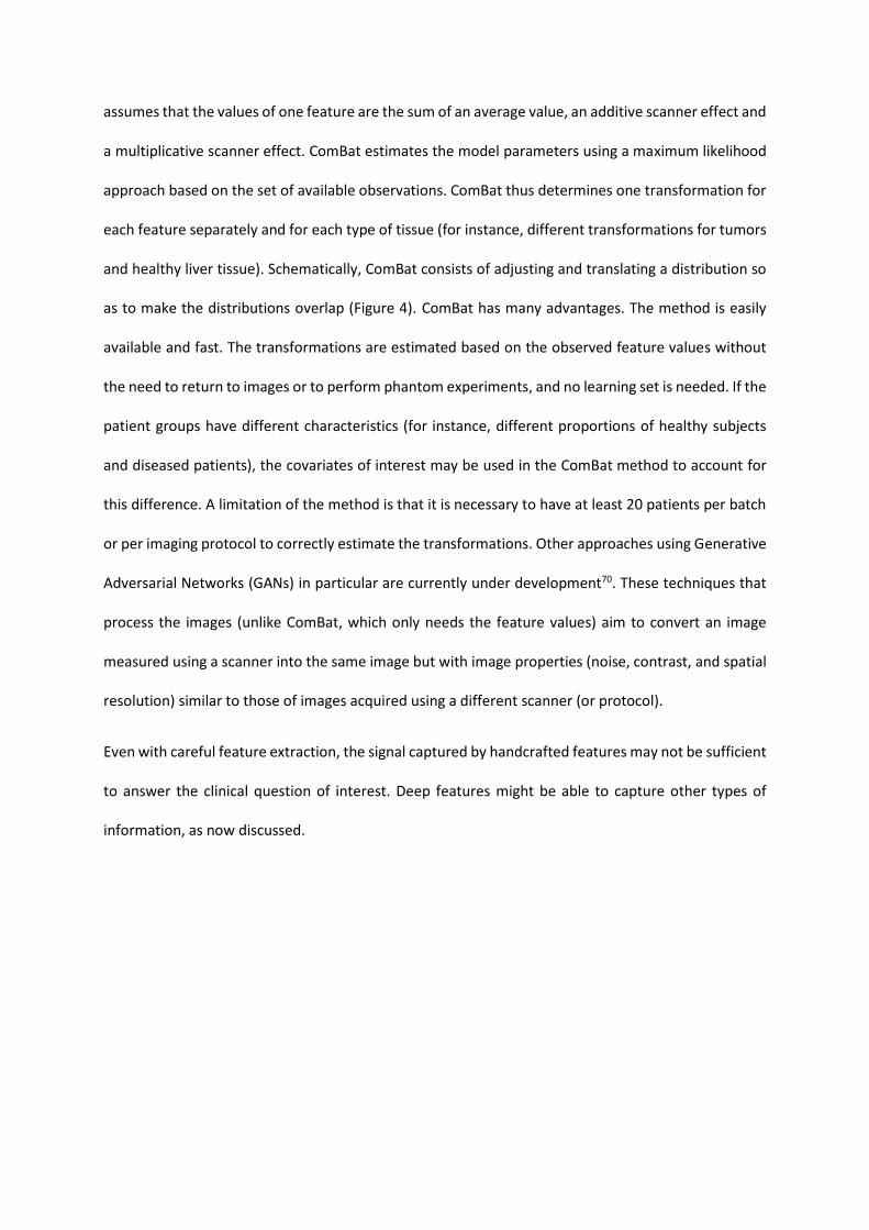
assumes that the values of one feature are the sum of an average value, an additive scanner effect and
a multiplicative scanner effect. ComBat estimates the model parameters using a maximum likelihood
approach based on the set of available observations. ComBat thus determines one transformation for
each feature separately and for each type of tissue (for instance, different transformations for tumors
and healthy liver tissue). Schematically, ComBat consists of adjusting and translating a distribution so
as to make the distributions overlap (Figure 4). ComBat has many advantages. The method is easily
available and fast. The transformations are estimated based on the observed feature values without
the need to return to images or to perform phantom experiments, and no learning set is needed. If the
patient groups have different characteristics (for instance, different proportions of healthy subjects
and diseased patients), the covariates of interest may be used in the ComBat method to account for
this difference. A limitation of the method is that it is necessary to have at least 20 patients per batch
or per imaging protocol to correctly estimate the transformations. Other approaches using Generative
Adversarial Networks (GANs) in particular are currently under development70. These techniques that
process the images (unlike ComBat, which only needs the feature values) aim to convert an image
measured using a scanner into the same image but with image properties (noise, contrast, and spatial
resolution) similar to those of images acquired using a different scanner (or protocol).
Even with careful feature extraction, the signal captured by handcrafted features may not be sufficient
to answer the clinical question of interest. Deep features might be able to capture other types of
information, as now discussed.
Figure 4: Harmonization using the ComBat method that realigns the distributions of feature values
obtained in different centers considering additive and multiplicative scanner effects.
Handcrafted vs deep features
The training of deep neural networks consists of iterative optimization of tunable network parameters.
In this process, deep features that help recognize these salient and persistent patterns become
encoded within the network. The type of features that the network learns is determined by the training
data, neural network architecture, and optimization algorithm.
This ability to learn disease-relevant deep features from the data is what gives deep learning its power.
In contrast to handcrafted features, automatic feature learning eliminates the need to perform feature
engineering or selection for a particular task. Feature selection is replaced by the selection of a deep

architecture. In addition, feature learning and predictive modeling can be performed in one step
(referred to as “end-to-end” training). Another possible advantage of deep learning approaches is that
neural networks might automatically identify the parts of the image that are most relevant for the task
of interest; in more advanced architectures, this is achieved using the so-called “attention” modules71.
Thus, there is no need to perform image segmentation prior to analysis, in contrast to handcrafted
features where an ROI/VOI needs to be specified for feature extraction. The associated drawback is
the need for added training data given the large collection of voxels being considered, as discussed
below.
The limitations of deep learning features are closely related to their advantages. First, not having to
perform feature selection comes at a price of requiring more data. Second, deep learning methods
often require significant tuning to perform adequately. Moreover, learned features may not have a
clear physical or biological meaning, so that the resulting model if often seen as a “black-box” without
any simple interpretation. Yet, the black box aspect of deep features and associated networks should
not be a show-stopper as more and more research is dedicated to providing means to decipher these
complex models. In addition, these models might ultimately provide evidence of sophisticated
information “hidden” in the data that could be turned into new hypotheses later amenable to testing
using dedicated experiments. In fields other than nuclear medicine, model-agnostic interpretation
methods have led to new discoveries, such as differences in the retina observed between men and
women72, or the importance of areas previously ignored by experts that were found to have prognostic
values (for instance areas within the stroma in pathological sections were found to have prognostic
value for mesothelioma patients73). Finally, learned features may capture image characteristics that
are not related to the diagnostic objective. For example, they may capture image properties related to
a particular scanner or imaging protocol74,75. Algorithmic methods that can examine which image
regions contribute to a decision produced by a neural network exist and will contribute to a better
understanding of the models, although that sometimes produce unreliable results76.

Since deep features are determined in large part by a particular dataset, they are subject to population
biases and may show poor descriptive performance when applied to a different dataset 77,78. The
relative generalization capacity between the deep and handcrafted radiomic features is still debated.
In this context, the advantage of handcrafted features is that their computation can be standardized;
however, no standards or standard libraries currently exist for deep radiomic features.
An important question to consider when planning an image analysis study is the relative expressive
power of deep and handcrafted radiomic features. Theory suggests that deep neural networks have
much greater expressive power than handcrafted radiomics. This follows from the universal
approximation theorem79 and implies that all handcrafted features are merely a small subset of deep
radiomic features. However, despite theoretical considerations, some handcrafted features may be
difficult for neural networks to learn in practice: there may be significant limitations with respect to
the required number of training samples or the number of neurons in the network. In other words,
simply because a neural network can act like any handcrafted feature does not mean that it can learn
to do so from given data (it may need significant depth in its layers and/or significant training data).
Because datasets are limited in practice and neural networks have finite sizes, they may be biases to
the types of deep radiomic features that can be learned from a given set of images. In a recent work,
we trained CNNs to function like common handcrafted features of the tumor intensity, texture and
shape80,81. In other words, we tested how well the deep networks can learn these features. We found
that CNNs were negatively biased in capturing shape information (Figure 5). This finding may have
significant implications for CNN-based quantitative medical image analysis since shape features
represent an important subset of handcrafted radiomics30. Thus, deep features may not be as effective
as handcrafted features at capturing and leveraging certain lesion properties that have previously been
associated with clinical outcomes. Therefore, handcrafted radiomic features appear to be
complementary to deep radiomic features rather than redundant – although additional studies in this
area are needed.

Figure 5: Feature learning errors for CNNs with 5, 7 and 9 convolutional layers, expressed in % of the
ground truth values of handcrafted features. The names of the tested handcrafted features are given
on the x-axis. The CNNs were trained on 4,000 synthetic 2D PET images containing realistic lesions
and tested on a separate set of 500 images.
Ultimately, the choice between handcrafted and deep radiomic features depends on the study
objectives and data availability. Handcrafted features can be recommended for inference studies,
where the objective is to establish a link between biologically meaningful features and a particular
clinical metric. These studies can be performed with a relatively low number of samples, which can be
determined based on the required power of the study. If a very large number of samples is available,
deep radiomics might achieve higher performance than models based on handcrafted features.
Summary
Radiomic analysis of PET images is a promising approach to extract subtler information and
continuously evolves with advances in artificial intelligence. Using deep learning methods, new
disease-specific deep features can also be learned directly from data and appear to complement
conventional handcrafted features. However, in order to create models that can be clinically translated
and benefit patients, investigators should be aware of the ins and outs of each step of the radiomic
pipeline. Particular attention must be paid to the comparison of the results obtained with state-of-the-

art approaches and to the findings previously reported in the literature in order to advance knowledge
in the field.

References
1. Gillies RJ, Anderson AR, Gatenby RA, Morse DL. The biology underlying molecular imaging in oncology: from genome to anatome and back again. Clin Radiol. 2010;65(7):517-521. doi:10.1016/j.crad.2010.04.005
2. Gillies RJ, Kinahan PE, Hricak H. Radiomics: images are more than pictures, they are data. Radiology. 2016;278(2):563-577. doi:10.1148/radiol.2015151169
3. Kuikka JT, Tiihonen J, Karhu J, Bergström KA, Räsänen P. Fractal analysis of striatal dopamine re-uptake sites. Eur J Nucl Med. 1997;24(9):1085-1090. doi:10.1007/BF01254238
4. McNitt-Gray MF, Wyckoff N, Sayre JW, Goldin JG, Aberle DR. The effects of co-occurrence matrix based texture parameters on the classification of solitary pulmonary nodules imaged on computed tomography. Computerized Medical Imaging and Graphics. 1999;23(6):339-348. doi:10.1016/S0895-6111(99)00033-6
5. Quantitative Imaging Biomarkers Alliance. Accessed May 18, 2021. https://www.rsna.org/research/quantitative-imaging-biomarkers-alliance
6. Reuzé S, Schernberg A, Orlhac F, et al. Radiomics in nuclear medicine applied to radiation therapy: methods, pitfalls, and challenges. Int J Radiat Oncol Biol Phys. 2018;102(4):1117-1142. doi:10.1016/j.ijrobp.2018.05.022
7. Zwanenburg A. Radiomics in nuclear medicine: robustness, reproducibility, standardization, and how to avoid data analysis traps and replication crisis. Eur J Nucl Med Mol Imaging. 2019;46(13):2638-2655. doi:10.1007/s00259-019-04391-8
8. Mayerhoefer ME, Materka A, Langs G, et al. Introduction to radiomics. J Nucl Med. 2020;61(4):488-495. doi:10.2967/jnumed.118.222893
9. Bizzego A, Bussola N, Salvalai D, et al. Integrating deep and radiomics features in cancer bioimaging. IEEE Conference on Computational Intelligence in Bioinformatics and Computational Biology (CIBCB). 2019; 18936077. doi:10.1101/568170
10. Peng H, Dong D, Fang M-J, et al. Prognostic value of deep learning PET/CT-based radiomics: potential role for future individual induction chemotherapy in advanced nasopharyngeal carcinoma. Clin Cancer Res. 2019;25(14):4271-4279. doi:10.1158/1078-0432.CCR-18-3065
11. Orlhac F, Nioche C, Soussan M, Buvat I. Understanding changes in tumor texture indices in PET: a comparison between visual assessment and index values in simulated and patient data. J Nucl Med. 2017;58(3):387-392. doi:10.2967/jnumed.116.181859
12. Martin-Gonzalez P, de Mariscal EG, Martino ME, et al. Association of visual and quantitative heterogeneity of 18F-FDG PET images with treatment response in locally advanced rectal cancer: A feasibility study. PLoS One. 2020;15(11):e0242597. doi:10.1371/journal.pone.0242597
13. Orlhac F, Thézé B, Soussan M, Boisgard R, Buvat I. Multiscale texture analysis: from 18F-FDG PET images to histologic images. J Nucl Med. 2016;57(11):1823-1828. doi:10.2967/jnumed.116.173708
14. Hoeben BAW, Starmans MHW, Leijenaar RTH, et al. Systematic analysis of 18F-FDG PET and metabolism, proliferation and hypoxia markers for classification of head and neck tumors. BMC Cancer. 2014;14:130. doi:10.1186/1471-2407-14-130
15. Bashir U, Weeks A, Goda JS, Siddique M, Goh V, Cook GJ. Measurement of 18F-FDG PET tumor heterogeneity improves early assessment of response to bevacizumab compared with the standard size and uptake metrics in a colorectal cancer model. Nucl Med Commun. 2019;40(6):611-617. doi:10.1097/MNM.0000000000000992
16. Buvat I, Orlhac F. The dark side of radiomics: on the paramount importance of publishing negative results. J Nucl Med. 2019;60(11):1543-1544. doi:10.2967/jnumed.119.235325
17. Boughdad S, Nioche C, Orlhac F, Jehl L, Champion L, Buvat I. Influence of age on radiomic features in 18F-FDG PET in normal breast tissue and in breast cancer tumors. Oncotarget. 2018;9(56):30855-30868. doi:10.18632/oncotarget.25762
18. Papp L, Pötsch N, Grahovac M, et al. Glioma survival prediction with combined analysis of in vivo 11C-MET PET features, ex vivo features, and patient features by supervised machine learning. J Nucl Med. 2018;59(6):892-899. doi:10.2967/jnumed.117.202267
19. Dirand A-S, Frouin F, Buvat I. A downsampling strategy to assess the predictive value of radiomic features. Sci Rep. 2019;9(1):1-13. doi:10.1038/s41598-019-54190-2
20. Liu X, Faes L, Kale AU, et al. A comparison of deep learning performance against health-care professionals in detecting diseases from medical imaging: a systematic review and meta-analysis. Lancet Digit Health. 2019;1(6):e271-e297. doi:10.1016/S2589-7500(19)30123-2
21. Lizarraga KJ, Allen-Auerbach M, Czernin J, et al. (18)F-FDOPA PET for differentiating recurrent or progressive brain metastatic tumors from late or delayed radiation injury after radiation treatment. J Nucl Med. 2014;55(1):30-36. doi:10.2967/jnumed.113.121418
22. Parmar C, Leijenaar RTH, Grossmann P, et al. Radiomic feature clusters and prognostic signatures specific for Lung and Head & Neck cancer. Sci Rep. 2015;5:11044. doi:10.1038/srep11044
23. Welch ML, McIntosh C, Haibe-Kains B, et al. Vulnerabilities of radiomic signature development: The need for safeguards. Radiother Oncol. 2019;130:2-9. doi:10.1016/j.radonc.2018.10.027
24. Lambin P, Leijenaar RTH, Deist TM, et al. Radiomics: the bridge between medical imaging and personalized medicine. Nat Rev Clin Oncol. 2017;14(12):749-762. doi:10.1038/nrclinonc.2017.141
25. Aerts HJWL, Velazquez ER, Leijenaar RTH, et al. Decoding tumour phenotype by noninvasive imaging using a quantitative radiomics approach. Nat Commun. 2014;5:4006. doi:10.1038/ncomms5006
26. Sanduleanu S, Woodruff HC, de Jong EEC, et al. Tracking tumor biology with radiomics: A systematic review utilizing a radiomics quality score. Radiother Oncol. 2018;127(3):349-360. doi:10.1016/j.radonc.2018.03.033
27. Collins GS, Reitsma JB, Altman DG, Moons KGM. Transparent reporting of a multivariable prediction model for individual prognosis or diagnosis (TRIPOD): the TRIPOD statement. Br J Cancer. 2015;112(2):251-259. doi:10.1038/bjc.2014.639
28. Mongan J, Moy L, Kahn CE. Checklist for Artificial Intelligence in Medical Imaging (CLAIM): A Guide for Authors and Reviewers. Radiology: Artificial Intelligence. 2020;2(2):e200029. doi:10.1148/ryai.2020200029
29. Buvat I, Orlhac F, Soussan M. Tumor texture analysis in PET: where do we stand? J Nucl Med. 2015;56(11):1642-1644. doi:10.2967/jnumed.115.163469
30. Zwanenburg A, Vallières M, Abdalah MA, et al. The Image Biomarker Standardization Initiative: standardized quantitative radiomics for high throughput image-based phenotyping. Radiology. 2020;295(2):328-338. doi: 10.1148/radiol.2020191145.
31. Zwanenburg A, Leger S, Vallières M, Löck S. Image biomarker standardisation initiative. arXiv:161207003 [cs, eess]. Published online December 21, 2016. doi:10.1148/radiol.2020191145
32. Foster B, Bagci U, Mansoor A, Xu Z, Mollura DJ. A review on segmentation of positron emission tomography images. Comput Biol Med. 2014;50:76-96. doi:10.1016/j.compbiomed.2014.04.014
33. Hatt M, Lee JA, Schmidtlein CR, et al. Classification and evaluation strategies of auto-segmentation approaches for PET: Report of AAPM task group No. 211. Med Phys. 2017;44(6):e1-e42. doi:10.1002/mp.12124
34. Klyuzhin IS, Gonzalez M, Shahinfard E, Vafai N, Sossi V. Exploring the use of shape and texture descriptors of positron emission tomography tracer distribution in imaging studies of neurodegenerative disease. J Cereb Blood Flow Metab. 2016;36(6):1122-1134. doi:10.1177/0271678X15606718
35. van Velden FHP, Kramer GM, Frings V, et al. Repeatability of radiomic features in non-small-cell lung cancer [(18)F]FDG-PET/CT studies: impact of reconstruction and delineation. Mol Imaging Biol. 2016;18(5):788-795. doi:10.1007/s11307-016-0940-2
36. Guezennec C, Bourhis D, Orlhac F, et al. Inter-observer and segmentation method variability of textural analysis in pre-therapeutic FDG PET/CT in head and neck cancer. PLoS One. 2019;14(3):e0214299. doi:10.1371/journal.pone.0214299
37. Yang F, Simpson G, Young L, Ford J, Dogan N, Wang L. Impact of contouring variability on oncological PET radiomics features in the lung. Sci Rep. 2020;10(1):369. doi:10.1038/s41598-019-57171-7
38. Klyuzhin IS, Fu JF, Shenkov N, Rahmim A, Sossi V. Use of generative disease models for analysis and selection of radiomic features in PET. IEEE Transactions on Radiation and Plasma Medical Sciences. 2019;3(2):178-191. doi:10.1109/TRPMS.2018.2844171
39. Beichel RR, Ulrich EJ, Smith BJ, et al. FDG PET based prediction of response in head and neck cancer treatment: Assessment of new quantitative imaging features. PLoS One. 2019;14(4):e0215465. doi:10.1371/journal.pone.0215465
40. Decazes P, Camus V, Bohers E, et al. Correlations between baseline 18F-FDG PET tumour parameters and circulating DNA in diffuse large B cell lymphoma and Hodgkin lymphoma. EJNMMI Res. 2020;10(1):120. doi:10.1186/s13550-020-00717-y

41. Cottereau A-S, Nioche C, Dirand A-S, et al. 18F-FDG PET dissemination features in diffuse large B-cell lymphoma are predictive of outcome. J Nucl Med. 2020;61(1):40-45. doi:10.2967/jnumed.119.229450
42. Seban R-D, Moya-Plana A, Antonios L, et al. Prognostic 18F-FDG PET biomarkers in metastatic mucosal and cutaneous melanoma treated with immune checkpoint inhibitors targeting PD-1 and CTLA-4. Eur J Nucl Med Mol Imaging. 2020;47(10):2301-2312. doi:10.1007/s00259-020-04757-3
43. Seban R-D, Nemer JS, Marabelle A, et al. Prognostic and theranostic 18F-FDG PET biomarkers for anti-PD1 immunotherapy in metastatic melanoma: association with outcome and transcriptomics. Eur J Nucl Med Mol Imaging. 2019;46(11):2298-2310. doi:10.1007/s00259-019-04411-7
44. Papp L, Rausch I, Grahovac M, Hacker M, Beyer T. Optimized feature extraction for radiomics analysis of 18F-FDG PET imaging. J Nucl Med. 2019;60(6):864-872. doi:10.2967/jnumed.118.217612
45. Crandall JP, Fraum TJ, Lee M, Jiang L, Grigsby PW, Wahl RL. Repeatability of 18F-FDG PET radiomic features in cervical cancer. J Nucl Med. 2021;62(5):707-715. doi:10.2967/jnumed.120.247999
46. Whybra P, Parkinson C, Foley K, Staffurth J, Spezi E. Assessing radiomic feature robustness to interpolation in 18F-FDG PET imaging. Sci Rep. 2019;9(1):9649. doi:10.1038/s41598-019-46030-0
47. Leijenaar RTH, Nalbantov G, Carvalho S, et al. The effect of SUV discretization in quantitative FDG-PET Radiomics: the need for standardized methodology in tumor texture analysis. Sci Rep. 2015;5:11075. doi:10.1038/srep11075
48. Orlhac F, Soussan M, Chouahnia K, Martinod E, Buvat I. 18F-FDG PET-derived textural indices reflect tissue-specific uptake pattern in non-small cell lung cancer. PLoS ONE. 2015;10(12):e0145063. doi:10.1371/journal.pone.0145063
49. Cottereau A-S, Meignan M, Nioche C, et al. Risk stratification in diffuse large B-cell lymphoma using lesion dissemination and metabolic tumor burden calculated from baseline PET/CT. Ann Oncol. 2021;32(3):404-411. doi:10.1016/j.annonc.2020.11.019
50. Brooks FJ, Grigsby PW. The effect of small tumor volumes on studies of intratumoral heterogeneity of tracer uptake. J Nucl Med. 2014;55(1):37-42. doi:10.2967/jnumed.112.116715
51. Orlhac F, Soussan M, Maisonobe J-A, Garcia CA, Vanderlinden B, Buvat I. Tumor texture analysis in 18F-FDG PET: relationships between texture parameters, histogram indices, standardized uptake values, metabolic volumes, and total lesion glycolysis. J Nucl Med. 2014;55(3):414-422. doi:10.2967/jnumed.113.129858
52. Pfaehler E, Mesotten L, Zhovannik I, et al. Plausibility and redundancy analysis to select FDG-PET textural features in non-small cell lung cancer. Med Phys. 2021;48(3):1226-1238. doi:10.1002/mp.14684
53. Shiri I, Maleki H, Hajianfar G, et al. Next-generation radiogenomics sequencing for prediction of EGFR and KRAS mutation status in NSCLC patients using multimodal imaging and machine learning algorithms. Mol Imaging Biol. 2020;22(4):1132-1148. doi:10.1007/s11307-020-01487-8

54. Guyon I, Weston J, Barnhill S. Gene selection for cancer classification using support vector machines. Machine Learning. 2002;46:389-422.
55. Tibshirani R. Regression shrinkage and selection via the Lasso. Journal of the Royal Statistical Society Series B (Methodological). 1996;58(1):267-288.
56. Parmar C, Grossmann P, Rietveld D, Rietbergen MM, Lambin P, Aerts HJWL. Radiomic machine-learning classifiers for prognostic biomarkers of head and neck cancer. Front Oncol. 2015;5:272. doi:10.3389/fonc.2015.00272
57. Papp L, Spielvogel CP, Rausch I, Hacker M, Beyer T. Personalizing medicine through hybrid imaging and medical big data analysis. Front Phys. 2018;6. doi:10.3389/fphy.2018.00051
58. Hastie T, Tibshirani R, Friedman J. The elements of statistical learning - data mining, inference, and prediction, Second Edition. Springer. Accessed June 18, 2021. https://www.springer.com/gp/book/9780387848570
59. Blinder SAL, Klyuzhin I, Gonzalez ME, Rahmim A, Sossi V. Texture and shape analysis on high and low spatial resolution emission images. In: 2014 IEEE Nuclear Science Symposium and Medical Imaging Conference (NSS/MIC). 2014:1-6. doi:10.1109/NSSMIC.2014.7430910
60. Yan J, Chu-Shern JL, Loi HY, et al. Impact of image reconstruction settings on texture features in 18F-FDG PET. J Nucl Med. 2015;56(11):1667-1673. doi:10.2967/jnumed.115.156927
61. Shiri I, Rahmim A, Ghaffarian P, Geramifar P, Abdollahi H, Bitarafan-Rajabi A. The impact of image reconstruction settings on 18F-FDG PET radiomic features: multi-scanner phantom and patient studies. Eur Radiol. 2017;27(11):4498-4509. doi:10.1007/s00330-017-4859-z
62. Ketabi A, Ghafarian P, Mosleh-Shirazi MA, Mahdavi SR, Rahmim A, Ay MR. Impact of image reconstruction methods on quantitative accuracy and variability of FDG-PET volumetric and textural measures in solid tumors. Eur Radiol. 2019;29(4):2146-2156. doi:10.1007/s00330-018-5754-y
63. Pfaehler E, van Sluis J, Merema BBJ, et al. Experimental multicenter and multivendor evaluation of the performance of PET radiomic features using 3-dimensionally printed phantom inserts. J Nucl Med. 2020;61(3):469-476. doi:10.2967/jnumed.119.229724
64. Reuzé S, Orlhac F, Chargari C, et al. Prediction of cervical cancer recurrence using textural features extracted from 18F-FDG PET images acquired with different scanners. Oncotarget. 2017;8(26):43169-43179. doi:10.18632/oncotarget.17856
65. Boellaard R, Delgado-Bolton R, Oyen WJG, et al. FDG PET/CT: EANM procedure guidelines for tumour imaging: version 2.0. Eur J Nucl Med Mol Imaging. 2015;42(2):328-354. doi:10.1007/s00259-014-2961-x
66. Kaalep A, Sera T, Rijnsdorp S, et al. Feasibility of state of the art PET/CT systems performance harmonisation. Eur J Nucl Med Mol Imaging. 2018;45(8):1344-1361. doi:10.1007/s00259-018-3977-4
67. Johnson WE, Li C, Rabinovic A. Adjusting batch effects in microarray expression data using empirical Bayes methods. Biostatistics. 2007;8(1):118-127. doi:10.1093/biostatistics/kxj037

68. Fortin J-P, Cullen N, Sheline YI, et al. Harmonization of cortical thickness measurements across scanners and sites. Neuroimage. 2018;167:104-120. doi:10.1016/j.neuroimage.2017.11.024
69. Orlhac F, Boughdad S, Philippe C, et al. A postreconstruction harmonization method for multicenter radiomic studies in PET. J Nucl Med. 2018;59(8):1321-1328. doi:10.2967/jnumed.117.199935
70. Xie Z, Baikejiang R, Li T, et al. Generative adversarial network based regularized image reconstruction for PET. Phys Med Biol. 2020;65(12):125016. doi:10.1088/1361-6560/ab8f72
71. Oktay O, Schlemper J, Folgoc LL, et al. Attention U-net: Learning where to Look for the pancreas. arXiv:180403999 [cs]. Published online May 20, 2018. Accessed March 16, 2021. http://arxiv.org/abs/1804.03999
72. Holm EA. In defense of the black box. Science. 2019;364(6435):26-27. doi:10.1126/science.aax0162
73. Courtiol P, Maussion C, Moarii M, et al. Deep learning-based classification of mesothelioma improves prediction of patient outcome. Nat Med. 2019;25(10):1519-1525. doi:10.1038/s41591-019-0583-3
74. Zech JR, Badgeley MA, Liu M, Costa AB, Titano JJ, Oermann EK. Variable generalization performance of a deep learning model to detect pneumonia in chest radiographs: A cross-sectional study. PLOS Medicine. 2018;15(11):e1002683. doi:10.1371/journal.pmed.1002683
75. Badgeley MA, Zech JR, Oakden-Rayner L, et al. Deep learning predicts hip fracture using confounding patient and healthcare variables. npj Digital Medicine. 2019;2(1):1-10. doi:10.1038/s41746-019-0105-1
76. Hooker S, Erhan D, Kindermans P-J, Kim B. A Benchmark for interpretability methods in deep neural networks. arXiv:180610758 [cs, stat]. Published online November 4, 2019. Accessed March 16, 2021. http://arxiv.org/abs/1806.10758
77. Chen IY, Szolovits P, Ghassemi M. Can AI help reduce disparities in general medical and mental health care? AMA Journal of Ethics. 2019;21(2):167-179. doi:10.1001/amajethics.2019.167
78. Mårtensson G, Ferreira D, Granberg T, et al. The reliability of a deep learning model in clinical out-of-distribution MRI data: A multicohort study. Medical Image Analysis. 2020;66:101714. doi:10.1016/j.media.2020.101714
79. Hornik K, Stinchcombe M, White H. Multilayer feedforward networks are universal approximators. Neural Networks. 1989;2(5):359-366. doi:10.1016/0893-6080(89)90020-8
80. Klyuzhin I, Rahmim R. Shape analysis in PET images using convolutional neural nets: limitations of standard architectures. Accessed March 16, 2021. https://virtual.aapm.org/aapm/2020/eposters/301769/ivan.klyuzhin.shape.analysis.in.pet.images.using.convolutional.neural.nets.html?f=menu%3D17%2Abrowseby%3D8%2Asortby%3D2%2Amedia%3D2%2Atopic%3D23585
81. Klyuzhin IS, Xu Y, Ortiz A, Ferres JML, Hamarneh G, Rahmim A. Testing the Ability of Convolutional Neural Networks to Learn Radiomic Features. medRxiv. Published online September 23, 2020:2020.09.19.20198077. doi:10.1101/2020.09.19.20198077