random graphs and social networks: an economics perspective · random graphs and social networks:...
TRANSCRIPT
RANDOM GRAPHS AND SOCIAL NETWORKS:
An Economics Perspective
by
Yannis M. Ioannides
Department of Economics, Tufts University
June 22, 2015
Abstract
This eclectic review of current research on networks emphasizes three strands of the lit-
erature on social networks. The first strand is composed of models of endogenous network
formation from both the economics and the computer science literature. The review high-
lights the sensitive dependence of the topology of endogenous networks on parameters of the
behavioral models employed.
The second strand draws from the recent econophysics literature in order to review the
recent revival of interest in the random graph theory. This mathematical tool allows one to
study social networks that result from uncoordinated random action of individuals in setting
up connections with others. The review explores a number of examples to assess the potential
of recent research on random graphs with arbitrary degree distributions in accommodating
more general behavioral motivations for social network formation.
The third strand focuses on a specific model of social networks, Markov random graphs,
that is quite central in the mathematical sociology and spatial statistics literatures but little
known outside those literatures. These are random graphs where the events that different
edges are present are dependent, if edges are incident to the same node, and independent,
otherwise. The paper assesses the potential for economic applications with this particular
tool. The paper concludes with an assessment of observable consequences of optimizing
behavior in networks for the purpose of estimation.

Contents
1 Introduction 4
2 Models of Endogenous Network Formation 7
2.1 A Simple Model of Network Formation . . . . . . . . . . . . . . . . . . . . . 9
2.2 The economics literature on network formation . . . . . . . . . . . . . . . . . 12
2.3 Value of Direct Contacts and The Co-authoring Model . . . . . . . . . . . . 20
3 Random Graph Theory: Old and New 22
3.1 The Erdos and Renyi Model . . . . . . . . . . . . . . . . . . . . . . . . . . . 22
3.2 The Revival of Random Graph Theory . . . . . . . . . . . . . . . . . . . . . 24
3.3 Random Graphs with Arbitrary Degree Distribution . . . . . . . . . . . . . . 28
3.4 Emergence of Giant Component . . . . . . . . . . . . . . . . . . . . . . . . . 30
3.5 Sizes of Interconnected Groups of Agents . . . . . . . . . . . . . . . . . . . . 31
3.6 Trade in Differentiated Products . . . . . . . . . . . . . . . . . . . . . . . . 34
3.7 Graphical Economies: Extension of the Arrow–Debreu Model . . . . . . . . . 38
3.7.1 Other Models of Interactions with Direct Neighbors . . . . . . . . . . 40
3.8 Social Networks versus Other Networks . . . . . . . . . . . . . . . . . . . . . 41
3.9 Centrality and Searchability of Random Graphs . . . . . . . . . . . . . . . . 43
3.10 Applications with Models of Job Matching . . . . . . . . . . . . . . . . . . . 45
4 Markov Random Graph Models of Social Interactions 47
4.1 The Frank–Strauss Model of Markov Random Graphs . . . . . . . . . . . . . 49
5 Observable Consequences of Optimizing Behavior in Networks 53
5.1 Actions as Outcomes from Games in Finite Networks . . . . . . . . . . . . . 53
2

5.2 Actions in Large Networks . . . . . . . . . . . . . . . . . . . . . . . . . . . . 54
5.3 Implications for Behavioral Modelling . . . . . . . . . . . . . . . . . . . . . . 55
6 References 59
7 APPENDIX 69
7.1 Analytics of the Modern Approach to Random Graphs with Arbitrary Degree
Distributions . . . . . . . . . . . . . . . . . . . . . . . . . . . . . . . . . . . 69
7.1.1 Emergence of Giant Component . . . . . . . . . . . . . . . . . . . . . 71
7.1.2 Sizes of Groups of Interconnected Agents? . . . . . . . . . . . . . . . 72
7.2 The Case of Directed Graphs . . . . . . . . . . . . . . . . . . . . . . . . . . 73
7.2.1 An Example with the Number of In-edges and Out-edges Being De-
pendent . . . . . . . . . . . . . . . . . . . . . . . . . . . . . . . . . . 74
7.2.2 Emergence of a Giant Component . . . . . . . . . . . . . . . . . . . . 75
7.2.3 Bipartite Graphs and their Application to Multilateral Matching . . . 76
3
1 Introduction
This paper1 examines stochastic social networks by means of models that allow us to make
the state of entire networks, rather that of individual agents, the subject of analysis. It
explores the recent econophysics, computer science and sociology literatures in addition to
that in economics and emphasizes views of social networks as outcomes of economic decisions
of individuals.
The literature on social network analysis that aims at description and analysis of prop-
erties of social structures is an established one in sociology. Although the stochastic version
of that literature has borrowed tools from spatial statistics and random graph theory, it is
fair to say that the patterns of borrowing suggests occasional and decisive influence rather
than continuous interplay. Random graph theory, of course, while it has been perceived from
its inception as a purely mathematical subject [ Erdos and Renyi (1959; 1960) ], has con-
tinuously lent itself to use by mathematical sociologists, electrical engineers and computer
scientists.
The use that economists have made of these theories is rather limited. This is quite sur-
prising for a number of reasons and not so surprising for other reasons. For example, many
economic applications do not emphasize the individual and simply aggregate over a number
of people, or work with a “representative individual.” As Kirman (1992; 2002) argues, the
notion of a representative individual can be quite deceptive, when the aggregate behaves
qualitatively different from the sum of individuals’ behavior. Some of the tools developed
by the literature that is discussed in this paper lend themselves well to such a task, as
aggregation with a large number of agents may lead to phase transition. Other economic ap-
plications, as in models of strategic interactions and with few exceptions, essentially assume
small groups of actors, within which every one interacts with every one else, and thus no
issues of aggregation and phase transitions arise. Still others, such as search and matching,
do emphasize economic applications with inherent discreteness and do lead to aggregation.
Yet, at the end, that literature typically appeals to large numbers and summation.
There is another aspect of the search literature that is worth pondering. That literature
4

has analyzed successfully how agents find one another in order to carry out transactions.
Individuals looking for work know that jobs may be available at various firms but they
need to find out which ones may be acceptable to them. Firms looking for employees need
to make their openings known to all those who are potentially interested in them. Job
search by individuals and firms’ efforts to fill vacancies have been studied extensively by a
large body of literature that amounts to an important part of modern macroeconomics; see
Pissarides (2001). Interactions between such discrete entities as individuals and firms are
an interesting instance of social interactions. Yet, the search literature has not emphasized
the web of relationships between firms and workers and among workers who have shared
experiences in dealing with the same firms, and firms in dealing with the same workers,
that may develop out of shared employment experiences. The fact that such experiences
may lead to employment referrals in the future has been recognized, but the role of webs of
relationships may not be easy to analyze by means of representative individual models or by
models that involve summation and large numbers.
The paper starts in section 2 with a review of models of networks formation. I am not
attempting to duplicate two recent papers, Goyal (2003) and Jackson (2003), nor Jackson’s
magisterial review of the literature [Jackson (2005)], that have eloquently reviewed substan-
tial portions of the same literature as the one discussed here. Instead, I aim here at exploring
methodological trends in the interface between the economics and the computer science lit-
erature and how they have been influenced by (often different) stylized facts that both those
literatures have focused on. I eschew an in-depth analysis of labor market applications, be-
cause I have discussed them elsewhere [Ioannides and Loury (2004)]. The particular strand
of the computer science literature that I discuss here has a natural economic motivation,
in that it is considering the emergence of the world wide web as an endogenous object [
Papadimitriou (2003) ]. The web’s various properties, including alleged power laws for the
number of nodes that are incident to each edge, topological properties of the entire network
and others such searchability properties [ Kleinberg (2000); Newman (2003) ] follow from
endogenous interactions between individuals and technological systems much more than any
previously designed system. The very simple economic model of network creation with which
5

that section starts complements the economics research on network formation. The fact that
most recent applications of economic tools to studying network formation are generally cast
in terms of deterministic models suggests that network formation in stochastic environments
also deserves attention.
Next I turn in section 3 to a review of random graph theory which while originating in
Erdos and Renyi, op. cit., has recently been developing as a source of models of networks
of social contacts, or social networks, for short. The presentation traces the applications of
the theory by a small number of economic applications and then discusses the shortcomings
of the early random graph models. It is an essential part of that theory that the events
that there exist contacts between different individuals are independent. It is critical to be
able to allow for dependence in the presence of contacts between different individuals, since
such dependence may be an outcome of individual responses to correlated random factors
or to selection and sorting. It may also be a key outcome in deterministic models of social
networks.
The remainder of that section of the paper turns to a recent revival of interest in random
graph theory. Recent developments have generalized the original Erdos – Renyi model, and
thus should allow newer applications in understanding social networks and social interactions
more generally. To do so, I draw from the recent econophysics literature on random graphs
and social networks, which offers the most direct generalization of the classic random graph
model ala Erdos and Renyi. This includes notable developments that have recently summa-
rized very eloquently by Newman (2002) and Newman (2003d) and by others. As we shall see
in more detail, some of the strands of this newer literature, which is also linked with related
computer science literature, has been motivated by a desire to explain observable features
of real life networks, like the WWW. These properties generalize the restrictive assumptions
of the original random graph model ala Erdos and Renyi. In fact, much research within the
econophysics community has been aimed at explaining a number of stylized facts regarding
measures of man-made networks, including the WWW, coauthorship and citation networks,
and others because of the failure of the Erdos and Renyi random graph model to explain
them satisfactorily. Still, the econophysics literature on random graphs and networks gener-
6
ally lacks clear behavioral motivations of the sort that economists are typically accustomed
to.
Section 4 discusses a class of models that address a key weakness of the modern approach
to modelling real world networks, namely the modelling of transitivity. This important prop-
erty of endogenous social networks may be handled by Markov random graphs, which treat
entire social networks as stochastic objects. This model is well known in mathematical so-
ciology and spatial statistics. It originates in Frank and Strauss (1986) and Strauss (1986)
and has ever since received continuous attention by the mathematical sociology literature
[Hagsberg (2002); Wasserman et al. (2004)]. That section provide links of Markov random
graphs in the Frank–Strauss style with random graph theory in the Erdos–Renyi style by
means of a particular application of random graph theory, and its implications for the dy-
namics of adjustment in social interaction and other related models. The paper concludes
by pondering on the scope of the broadly interdisciplinary research on endogenous network
formation.
2 Models of Endogenous Network Formation
A series of innovative recent papers model the endogeneity of links among originally isolated
agents. Goyal (2003) and Jackson (2003), provide eloquent reviews of various aspects of the
literature on endogenous network formation. Within this recent literature, especially note-
worthy are papers by Bala and Goyal (2000a), Jackson and Watts (2002a; 2002b), Jackson
and Wolinsky (1996), and Watts (2001). These authors embed endogenous network forma-
tion in the tradeoff between the value to different agents from existence of interconnections
with other agents and the costs agents themselves incur from initiating connections. We
review here some key findings that have been established by this literature. I start from the
simplest possible model in the literature, Fabrikant et al. (2003), which highlights essential
issues and tradeoffs in endogenous network formation. The fact that this particular paper,
which is closely related to Jackson and Wolinsky (1996), originates in the computer sci-
ence literature underscores a significant interplay between that field and economics. This is
7

quite natural in view of the recent interest by computer scientists in studying game-theoretic
formulations of network-based resource allocation problems.
I introduce some basic terminology and notation regarding graphs and networks. To
start with, the terms graphs and networks are really synonyms for our purposes, although
the term graph appears to be used exclusively by mathematicians and of course by others as
well, but the terms graphs and networks are used almost interchangeably by all other fields.
Let the elements of a set I = 1, . . . , I represent individuals. It is individuals who are
the decision makers and thus objects of analysis in most of the applications in the present
paper. Established communication, social relations, or social interactions between any two
individual members of I are defined by an undirected graph G(V ,E), where: V is the set of
vertices, V = v1, v2, . . . , vI, an one-to-one map of the set of individuals I onto itself (the
graph is labelled), and I = |V | is the number of vertices (nodes), also known as the order of
the graph; E is a proper subset of the collection of unordered pairs of vertices, q = |E| is the
number of edges, and is also known as the size of the graph. We say that agent i interacts
with agent j if there is an edge between nodes i and j. Let ν(i) define the local neighborhood
of agent i : ν(i) = j ∈ I|j = i, i, j ∈ E. The number of i’s neighbors is the degree of
node i : di = |ν(i)|.
Graph G(V ,E) may be represented equivalently by its adjacency matrix, Γ, an I × I
matrix whose (i, j) element,γij, is equal to 1, if there exists an edge connecting agents i and
j, and to 0, otherwise. For undirected graphs (and most of the graphs I consider here are
undirected), matrix Γ is symmetric and positive, and thus its spectral properties which are
important in the study of social interactions, are well understood. When appropriate in
the present paper, the adjacency matrix Γ will be defined as a random matrix with generic
realization Γ. The entries of the adjacency matrix γij would be binary random variables in
that case, with the most interesting case being when different γij’s may be considered as
dependent random variables, as in the case of the Markov random graph model.
8
2.1 A Simple Model of Network Formation
Fabrikant et al. (1003) consider a model with agents I who build connections with each
other. Their decisions create a undirected graph, G(V ,E), which is to be treated as an
endogenous outcome. Once a connection between two agents has been established, it may
be used by all other agents via the two agents at its two ends. The strategy space of agent
i is the set Si = 2I−i. We denote by G(s) the graph resulting from all agents’ employing
strategies s = (s1, . . . , sI) ∈ S1 × . . . × SI . The cost incurred by agent i when all agents
employ strategy s is assumed to be additive in the cost of the number of connections, |si|,
that agent i herself builds with other agents, and in the sum of the costs each agent i must
incur in order to reach all other agents through G(s):
ci(s) = α · |si|+I∑j=1
dG(s)(i, j), (1)
where dG(s)(i, j) denotes the distance between agents i and j within the graph G(s). Note
that parameter α, the relative importance of agent i’s direct links with other agents, is the
only parameter in the model.
Agents seek to minimize their objective functions, given by (1). It is easy to characterize
Nash equilibria and the social optimum for this simple model. They depend critically on
the magnitude of α, the cost of a link. If α < 1, then the complete graph (the maximal
clique) is the only Nash equilibrium. The intuition is straightforward: any Nash equilibrium
cannot miss an edge whose inclusion would reduce the second term in the objective by
more than it would add to the cost. It is also the social optimum, in that it minimizes
α · |E|+∑Ii,j dG(s)(i, j). For 1 ≤ α < 2, the graphs that are Nash equilibria have diameter at
most 2. The social optimum is still the complete graph, and the star is a Nash equilibrium.
For α ≥ 2, the star is a Nash equilibrium, but there may others, too. The social optimum
continues to be the star. Generally, intuition suggests that for sufficiently high values of
α, Nash equilibria would be trees, because they offer a lower value for the second term in
the definition of an agent’s cost according to (1). Yet, there does not appear to be a proof
of this, and in fact Fabrikant et al., op. cit., offer it as a conjecture. It is clear that the
presence of graph distance in the objective function (1) is quite critical for the properties of
9

the equilibrium outcomes in this formulation.
A number of remarks are in order. First, we note that while all equilibrium outcomes are
actually connected graphs, it is not obvious that in a decentralized setting there would be a
priori agreement as to where the star would be centered. The simplicity of the solution to this
problem provides an important benchmark for endogenous network formation. Second, for
both the computer science and the economics literatures, it is of critical importance whether
Nash equilibria may be arrived at through the sort of perturbation of best responses that
economists are familiar with and at a reasonable cost. It is of particular consequence to
computer scientists that such a perturbation analysis, whereby one starts with a strategy
and then replaces it by a player’s best response, turns out to be NP − hard; see ibid., p.
348. Third, the prominence of the star as an equilibrium outcome prompts us to consider its
robustness in more general settings. Several concerns immediately arise: one, it is vulnerable
in a stochastic setting where connections may fail; two, it is prone to congestion; and three,
a more general economic model should express benefits associated with different graphs and
not just costs.
Fabrikant et al. (2002) work with a related model which, however, emphasizes degree
distributions and other topological properties of resulting graphs at the limit when the
number of agents is large. Their model produces a power law distribution in certain graph
measures, which are of interest in the context of the Internet topology, precisely when new
nodes that randomly appear choose optimally their connections with an existing network.
2 Entering nodes seek to minimize their distance to the “center” of the existing network
topology plus the weighted Euclidean distance to an existing node. If distances from the
existing node, which a new node chooses to connect with, to other nodes in an existing
network, are given a larger relative weight in the objective of the optimization problem,
then the resulting network is a star. If, on the other hand, the weight grows at least as fast
as the square root of the size of the entire graph, then the resulting degree distribution is
exponential. For the in-between values, the resulting degree distribution tends to a power
law. In this model, the graph is defined in a two dimensional continuous space and is bounded
within a unit square within it.
10
Specifically, Fabrikant et al. (2002) study the evolution of the network as agents i =
1, 2, . . . , arrive uniformly at random and choose one of the existing other agents, j, j =
1, . . . , i− 1, to connect with. Each entering agent i chooses agent j to link with to so as to
minimize
fi(j) = a · dij + hj, (2)
where dij denotes the Euclidean distance between i and j, and hj a measure of the “centrality”
of the agent j within the final graph formed by the decision of agent i. This measure could be
the average graph distance from all other agents, the maximum such distance or the graph
distance to the center of the tree, the number of hops from i to 1 in Ti, which is actually
the measure they use to prove their results. The evolving endogenous networks are trees,
T0, T1, . . . , and Ti consists of Ti−1, with the agent i and the connection [i, j] added. Here the
parameter a denotes the cost of connecting to agent j relative to the importance of centrality,
which has a coefficient of 1.
The solution depends critically on the magnitude of parameter a, which is actually treated
as a function of I. If it is relatively small, a < 1/√2, that is distances to all other nodes
are relatively more important, then the resulting network TI is a star, centered at the node
associated with agent 1. Regarding the associated degree distribution, this solution is the
extreme version of a power law, where all agents are connected with the single original agent.
If a = Ω(√I) (that is, it is more than some constant multiple of
√I), that is the weight
attached to distance to the nearest node grows sufficiently fast with the number of agents,
the degree distribution of TI is exponential. That is, the expected number of agents that
are connected to at least K other agents is bounded above by I2e−cK . Finally, if a ≥ 4, and
a = o(√I) (that is, for in-between values as a may vary I but grow slower than
√I, as I
grows very large), then the degree distribution of TI is a power law : the expected number
of agents who are connected with at least K other agents is greater than c ·(KI
)−β, where
c, β are constants that may depend on a.
Fabrikant et al. have growth of the Internet in mind in building their model. The
stylized facts, as established by Faloutsos et al. (1999), provide empirical support for a power
law, although much of the power law literature, a.k.a. “scale-free” laws, has taken pain to
11

emphasize the universality of power laws. This clearly appears to have been exaggerated.
Therefore, the dependence of the distribution parameters in the above results is obviously a
drawback. We return below in Section 5 to these empirical findings.
An economic interpretation of this result would be in terms of preferential attachment.
Those agents who have arrived early are more likely to have more connections with others and
be near others, reducing the hop cost. A significant feature of this result is that preferential
attachment is derived from more primitive assumptions, relative to other work where it is
just assumed as a realistic feature of real-world networks. Most importantly, Fabrikant et al.
(2002) appear to offer the first purely behavioral model that leads to emergence of a power
law for the degree distribution of nodes in an endogenously formed network. We return to
this issue further below.
2.2 The economics literature on network formation
The models in the economics literature that also make links endogenous by means of strategic
considerations are somewhat more general than their computer science counterparts in a
number of respects, but at the same time focus on slightly different issues. Some of the
papers are often more explicit regarding building of links between two originally isolated
individuals. For example, some of the papers require that those to be directly connected both
consent to it, whereas severance can be done unilaterally. Links may directed (asymmetric,
in Bala and Goyal’s terminology) or undirected. Links between agents are interpreted as
information channels. A directed link (i, j) denotes that agent i has access to agent j’s
information and does not imply that j has access to i’s. For example, i could have access to
j’s web-site or have access to exact URL for a particular document. In fact, directed links
are a key feature of the web graph. Consequently, for every possible directed link that an
individual is contemplating, there is its counterpart in the opposite direction as well as a
multitude of indirect links that accomplish the same informational effect though at a higher
cost. Undirected links may model connections like that provided by telephone.
Most of the papers in the economics literature assume that the utility each agent de-
12

rives from participating depends additively on the total number of other agents an agent is
connected with, minus the costs of maintaining the connections that one builds on her own.
Some authors make an allowance for proximity to others by means of a decay factor that
depends on the number of intervening agents.
Bala and Goyal (2000) assume that individual i’s payoff is strictly increasing in the
number of agents “observed” by i, µi(g), that is other agents with whom i has formed direct
links or is linked to indirectly through others, and strictly decreasing in the number of other
agents that i has built direct links with, µdi (g) = |si|. In the special case when each individual
possesses information which is of value V, which may be normalized and set equal to 1, to
each of every other agent and to himself, the benefits from the information possessed by
those whose information she accesses directly or indirectly are proportional to µi(g). If an
agent incurs linear costs of forming direct links, which are denoted by c per link, then the
net benefit to agent i is
Πi(g) = µi(g)− cµdi (g). (3)
If c < 1, then agent i will be willing to form a link with agent j for the sake of that agent’s
information alone. If 1 < c < I − 1, then agent i will want agent j to have access with more
than one other agent in order to be induced to form a link with j. If c > I − 1, then the cost
of a link exceeds the benefit of information to the entire society. In that case, it is dominant
strategy for i not to form a link with any player.
The empty network is a Nash equilibrium. Bala and Goyal show that when agents’
objective is as Πi(g) above, then a strict Nash network is either the wheel, whereby each
agent forms exactly one link, or the empty network. In other words, information is either
shared with everyone with the minimum number of connections per agent that makes this
possible, which implies the wheel, which would be the unique case with linear payoff if c < 1,
or along with the empty network, if 1 < c < I − 1; or there is no sharing when c > I − 1.
We note the difference in equilibrium outcomes from the Fabrikant et al. formulation of the
network formation game. Their formulation assigns weight to centrality as such, which of
course penalizes the wheel. It is connectedness, however, that plays a similar role in the
Bala–Goyal formulation.
13

In view of the dramatically restricted set of Nash networks, the following question arises:
will a society of agents thus motivated self-organize into equilibrium outcomes? Bala and
Goyal study the dynamics of link formation by assuming a naive best response rule with
inertia. That is, an agent may choose, with fixed probabilities, either a myopic pure strategy
best response, or the same action as in the previous period. Inertia ensures that agents
will not mis-coordinate perpetually. Bala and Goyal show that irrespective of the number
of agents and by starting from any initial pattern of interconnections, the dynamic process
indeed self-organizes, by converging with probability 1, and in finite time, to the appropriate
(for the respective parameter values) unique limit network. The limit is the set of strict Nash
networks of the one- shot game, which become the set of absorbing states of the dynamic
process. Technically, the rules of individual behavior define a Markov chain on a state space
consisting of all networks, whose absorbing states are the Nash equilibria of the one-shot
game.
These results may be generalized by restricting the information available to agents, that
is by assuming only local information – each agent knows the residual set of all those she is
connected with, that is those her neighbors can access without using links to her – and by
allowing observation of successful agents – there is some chance that she receives information
from a “successful” agent, that is a person who observes the largest subset of people in the
economy without assistance from her own links. The results continue to hold when the payoff
to each agent is assumed to be strictly increasing in the number of other agents she observes,
and strictly decreasing in the number of links that she forms. In that case, the unique efficient
architecture is the wheel, if an agent is better off by observing all others and forming one link,
when she would enjoy utility Π(I, 1), than if she is on her own, when she would enjoy utility
Π(1, 0); it is the empty network, otherwise, that is, when Π(I, 1) < Π(1, 0), where I denotes
the number of agents. Again, the dynamic process self-organizes if Π(k + 1, k) > Π(1, 0),
for some k ∈ 1, 2, . . . , I − 1, in which case the limit is the wheel, if Π(k + 1, k) < Π(1, 0),
∀k ∈ 1, 2, . . . , I − 1, in which case the limit is either the wheel or the empty network.
Although networks with directed links are important — it is a critical feature of the
WWW that is directional — and are attracting considerable attention, the study of undi-
14

rected links is also interesting. Bala and Goyal also study undirected links, which as men-
tioned above accommodate two-sided information flows. This case best represented by a
phone call connection, where a person initiates a call to another person and incurs its cost,
but both parties benefit from the exchange. They show that when the typical agent has
a general payoff which is increasing in µi(g), the total number of others an individual
is linked with directly or indirectly, and decreasing in the number of direct links, µdi (g),
Πi(g) = ϕ(µi(g), µdi (g)), then a strict Nash network is either a center-sponsored star (the
agent who initiates it serves as center and pays for the costs of links), or the empty network.
The fact that the star is a prominent architecture here, both as the efficient network and
the limit for self-organization, suggests that network architecture is sensitive to the nature
of information technology. We note that this result is equivalent to Fabrikant et al. (2003),
whose problem involves a cost minimization.
All of these results apply when the payoff is insensitive to the distance between agents in
the sense that direct and indirect connections contribute the same way to an agent’s payoff.
If the value of information possessed by an agent decays the further away others are from
her, then Bala and Goyal find it harder to precisely characterize strict Nash networks. While
the wheel continues, for some parameter values, to be the limit architecture the star also
appears as a limit, for other parameter values. This is, of course, not so surprising in view of
Fabrikant et al., (2003), discussed above, which assigns critical role to each agent’s network
distance from other agents. However, for some parameter values, especially when the decay
parameter is close to 1, other architectures are also associated with strict Nash equilibria,
such as “interlinked stars” and “rose-petals”. Self-organization is harder to characterize with
information decay, where limit results are obtained for parameter values that imply relatively
high costs of link formation.
Jackson and Wolinsky (1996) provide a model for two-sided link formation along with
a solution concept, pairwise stability: a network is pairwise stable, if no individual has an
incentive to delete a link that exists, and no pair of players have an incentive to form a link
15
that does not exist. The payoff to player i in network g is assumed to be
Πi(g) = 1 +∑
j∈N(i;g)
δdi,j(g) − µdi (g)c, (4)
where di,j(g) denotes the geodesic distance between agents i, j in the network, N(i; g) denotes
the set of all other agents whom i may reach via path in the network, µdi (g) the number
of agent i’s direct links in the network, and c the cost per link. With two-sided links (
the symmetric case ) pair-wise stable network outcomes may be, depending upon parameter
values, either the complete graph, where everyone is connected with everyone else, if 0 < c <
δ−δ2, or the Walrasian star, where everyone is connected to a single agent, if δ−δ2 < c < δ,
or no connections at all. We note that this result predates the Fabrikant et al. (2003).
Watts (1998) employs the same framework and extends it to a dynamic setting. She
obtains conditions under which networks with different architectures might form. In par-
ticular, if cost per link is very small, 0 < c < δ − δ2, then the process converges to the
complete network in finite time, with probability 1. If the cost is in an intermediate range,
δ − δ2 < c < δ, then the star network will emerge with positive probability, which decreases
with the number of players .
Jackson and Watts (2002a) study dynamic evolution of networks by means of sequences
of networks, which may come about as a result of myopic decisions of individuals in adding
and deleting links. They show that there always exists a pairwise stable network or a closed
cycle, that is when a number of different networks are repeatedly visited in some sequence.
They also introduce an evolutionary analysis of the dynamic network formation process,
where there exist a small probability of unintended changes ( “mutations” ). Using the same
mathematical tools as the ones employed by Young (1998), Jackson and Watts show that
networks, from those that are pairwise stable or belonging to cycles, that are harder to get
away from and easier to get to, are favored by the evolutionary process. However, they show
that even when the unique efficient graph is pairwise stable, it is not evolutionarily stable.
What sort of methodological arguments does this literature use in deriving results? The
arguments employed by Bala and Goyal in analyzing both asymmetric and symmetric links
involve intuitive steps that exploit the integer nature of the problem. This is also true for
16

Fabrikant et al. (2003). For example, in the case of undirected links, they Bala and Goyal
establish that a Nash network is either empty or connected. Then they show that if a player
n has a link with player j then no other player can have a link with j. That is, if two
agents, say i and j, can have a link with k, then one of them would be indifferent between
forming a link with k or with the other agent. Thus, n must be the center of the star.
Such arguments are appropriate for their setting, but make it hard to carry out comparative
statics (or dynamics) exercises, and do not lend themselves readily to handling heterogeneity
and uncertainty. Further research by Goyal and coauthors has enriched the set of outcomes
by appropriately specifying the objectives of agents and allowing for heterogeneity in the
value and the cost of connections, and for dependence on more complex characteristics of
network topology than just geodesic distances and number of direct links. We review next
some of these noteworthy developments.
Goyal and Joshi (2003) show that the interaction of individual incentives narrows down
the range of networks that may emerge at equilibrium. This range includes symmetric
(balanced) graphs with different degrees, exclusive group networks and stars. For a network
g, let g−i denote the network resulting from deleting agent i and all of her direct links,
and L(g−i) denotes the sum total of the degrees (links) of the rest of the agents: L(g−i) =∑j =i dj(g−i). Various examples discussed by Goyal and Joshi (2003) follow from different
specifications of the marginal benefit of an additional link of an agent, as a function of her
own degree and of the sum total of the degrees of all other agents. If the marginal benefit is
increasing in an agent’s own degree, then a pairwise-stable equilibrium network exists: it may
be empty, complete, or have the dominant group architecture (where one group of agents
forms a complete subgraph and a second group consists of isolated agents). Furthermore, if
the marginal return is increasing in the sum total of all others’ degrees, then the equilibrium
networks are undirected; if it is decreasing, they would be directed. This follows because
any two agents that link with others must also link with each other. If the marginal return
of an additional link is decreasing in an agent’s own degree and in the sum total of all
others’ degrees, then symmetric pairwise-stable equilibrium networks may not exist, and
asymmetric networks with sharp inequality in the number of links may assume the form
17

of star-like structures where linked agents have very unequal number of links. If, instead,
the marginal benefit is increasing in the sum total of all others’ degrees, then symmetric
equilibrium networks always exist.
Galeotti, Goyal and Kamphorst (2003) show that in models of strategic network for-
mation, heterogeneity with respect to the value of connections has a different effect from
heterogeneity with respect to the cost of links. The former affects the level of connectedness
of a network, while the latter affects both the level of connectedness of a network as well as
the architecture of the resulting components. When a society may be divided into distinct
groups, within each of which links are cheaper than links across to other groups, then inter-
connected stars are socially efficient and dynamically stable. This suggests that centrality,
star-sponsorship and small diameters are robust features of networks. All these studies show,
not surprisingly, that when agents’ objectives are more complex functions of network char-
acteristics, then the equilibrium network outcomes exhibit more complex structure. From
the perspective of the present paper, of course, this literature has been quite successful, in
that it has delivered analytical descriptions for the evolution of entire networks.
We eschew a discussion of job information networks because they are reviewed in detail
by Ioannides and Loury (2004). Another noteworthy area of applications is patterns in
international trade agreements that facilitate trade among certain countries and discourage
them among others may also lend themselves to similar considerations and have been largely
unexplored. We also pass up such applications, in part because they do not seem to fit the
sort of models involving large numbers of agents, which are essential for some of our results.
In concluding this section, it is important to note that the recent research on communica-
tion networks as models of social structure, which is reviewed here, has opened up important
avenues in hitherto virtually unexplored areas. An important payoff at stake here is linking
economics with the network-based theories of mathematical sociology. At the heart of the
sociology literature is a belief that network-based models are indispensable for modelling
more than just trivial social interactions. As White (1995) emphasizes, further theorizing
is likely to pay off even within sociology, where in spite of technical achievements in social
network measurements, modelling “network constructs have had little impact so far on the
18

main lines of sociocultural theorizing ... ” [ ibid., p. 1059 ]. White sees an important role
for studying social interactions through interlinking of different individual-based networks
associated with social discourse. It is also interesting that the literature in this area is de-
veloping fast. Especially noteworthy are a series of papers by Jackson and Rogers (2004;
2005).
Much of the economics literature has dealt with objective functions in individuals’ max-
imization problems that are not necessarily most suitable to the many different applications
network models are finding in the engineering literature. A particularly interesting model of
endogenous network formation is Johari et al. (2003). In their model, agents wish to connect
with others in order to route traffic among themselves. The resulting graph is directed. Each
agent, modelled by a node, wishes to route a given amount of traffic to some of the other
nodes and only cares whether the traffic eventually arrives at a destination. Each node incurs
a handling cost which is proportional to the volume of traffic through the node. Intuitively,
each agent prefers to be connected to all other agents, but also prefers that no other node be
connected with it, so that it not have to incur the costs of handling “transit” traffic through
itself. A bargaining model is developed, that is formalized in terms of the Jackson–Wolinsky
concept of pairwise stability, which is adapted as link stability. For each node i, a strategy
is a vector (pij, qji, ȷ = i), where pij ≥) is a bid from i to j to agree to forming a link (i, j),
and qji > 0 is a minimum acceptance value, that is the minimum payment node i is willing
to accept from j to agree to forming a link (j, i). A directed graph is formed G(I, A(s)),
defined in terms of the strategies of all nodes, s = (pij, qji, j = i), i, j ∈ I,
A(s) = (i, j) : i = j, pij ≥ qij.
Agent i receives a payoff of:
Ri(s) =∑
j:(j,i)∈A(s)pij −
∑j:(i,j)∈A(s)
pij − cifi(A)−∑
j∈wi(A)
Λij, (5)
where fi(A) is the volume of flow through i, Λ denotes the connectivity matrix, with Λii = 0,
Λij the cost incurred by i if j is unreachable from i, and wi(A) is defined as the set of nodes
which are unreachable from node i, given the links A(s). The paper characterizes solutions
to this problem by means of “contracts,” that allow each node to reach all other nodes for
19

which Λij > 0 and thus attain Λ-connectivity. The resulting links are minimal, in the sense
that no link can be removed without losing Λ-connectivity.
2.3 Value of Direct Contacts and The Co-authoring Model
An important aspect of social networks is the extent in which they are created as an outcome
of individuals’ myopic decisions. Two recent studies highlight this aspect. Goyal et al. (2003)
demonstrate that the “world of economics ” has become smaller since the early 1970s, as
measured by average “distance” between economists. Distance is measured in terms of
coauthorship: the distance between two economists who have co-authored at least a paper
is 1. The basic facts invoked by the paper are as follows. First, the number of economists
who published in journals has more than doubled from 1970 till 2000. Second, the largest
group of interconnected (in the above sense) economists, the “giant” component, grew from
15% to 40% of the total number of economists. Third, the average distance within the giant
component has fallen, while the clustering remains high. The 100 most linked (in terms of
co-authorships) economists in the 1990s produced an average of 38 papers of which almost
85% were co-authored. In contrast, the average number of papers per economist were 2.8,
and 40% of these were co-authored. A small number of “stars” are responsible for the giant
component: deleting the 5% most connected economists leaves less than 1% of the nodes in
the giant component. The topology of the network suggests that it is spanned by a hierarchy
of interconnected stars. Several features of the economics world seem to be quite different
from those of other sciences.
These facts pose problems for the standard theory. They reject most emphatically the
Erdos–Renyi random graph model. With 1.672 co-authors per person and 81,217 authors, the
probability of a random link is 0.00025, which is also approximately equal to the clustering
coefficient, in the case of the random graph model where connections are assumed to be
independent. However, the latter is computed to be about 0.157, and thus over 6000 times
larger than the random graph model would predict. The distribution od the number of
co-authorships is not Poisson and instead has a Pareto tail. The authors argue that the
20

basic preferential attachment model of Barabasi and associates does not describe well the
economics world. Furthermore, there is greater heterogeneity in the hierarchy levels of agents
with whom the central agent is linked, than in Ravasz and Barabasi (2003).
The authors propose a simple model that incorporates productivity differences across
individuals (with two types of agents being considered), there is a production function for
knowledge which is sensitive to the quality of co-authors and an incentives structure which
reward quality. The model is linear in the quality of research output and quadratic in the
costs of research effort and the number of co-authorships. In a world where there are few
high-productivity types the distribution of links and of the number of co-authors would be
very unequal. Links will arise between people who have many co-authors and who have
few co-authors. The authors interpret their results qualitatively as implying that stars arise,
that link well connected and poorly connected agents, and thus short distances are generated.
Only pairs of co-authors are examined in this study.
A different aspect of co-authoring is examined by Rosenblat and Mobius (2004), who
consider the impact of improvements in communication and transportation technologies on
self-selection in group formation. Lower communication costs decrease separation between
individuals but group separation may increase. So individuals’ being connected with others
facilitates spread of information about new technologies and job opportunities. At the same
time, heterogeneous agents may segregate by type. Data on economics co-authorships be-
tween US and foreign-based authors before and after the Internet revolution provide support
for this theory. Co-authoring has generally increased among economists. At the same time,
the Internet has enabled economists to be more selective and co-author with individuals who
may be located far from them geographically.
Marmaros and Sacerdote (2003) explore social interactions as measured by the volume of
emails among students and recent graduates of Dartmouth College. This study is significant
because roommates at Dartmouth are randomly assigned, and therefore the patterns of
interactions do not reflect any endogenous selection in terms of physical proximity. The
authors explain the volume of email between any two individuals in terms of racial, gender,
athletic and fraternity/sorority attributes, whether or not the respective individuals were
21
in the same class, had the same major or lived in the same dormitory, and interactions
among those variables. Their results suggest that same race is a very important explanatory
variable for the volume of email and so is to have lived in the same dorm. These results
underscore the importance of explaining the motivations for social interactions, which result
here in the presence of assortative mixing, that is based on personal characteristics as well
as past shocks in common.
3 Random Graph Theory: Old and New
Studying probabilistic aspects of social interactions would seem to lend itself to random
graph theory as a natural mathematical tool. Ever since economists became aware of the
existence of random graph theory ala Erdos and Renyi (1960; 1961) [but see Solomonoff
and Rapoport (1951) for an antecedent], it has been tempting to think of the emergence of
economic networks in terms of random graph theory. See Durlauf (1996), Kirman (1983),
Kirman et al. (1986), Ioannides (1990; 1997) for several examples of this approach. However,
all these works found it hard to motivate why it is that agents behave in the precise way that
is necessary to generate patterns of social connections that are associated graph features that
may be described by random graph theory, at least as originally developed. Still, economists
have yet to explore individuals’ motivation is seeking social contacts with others, at least as
far as this is understood by the psychology and social psychology literature.
3.1 The Erdos and Renyi Model
We first demonstrate how the key features of the Erdos–Renyi model are responsible for
some of its predictions. However, the Erdos–Renyi model does not seem to be supported by
the facts. Specifically, let GERI,p denote the ensemble of graphs with I vertices in which each
possible edge is present independently of any other edge and with probability p, and absent
with probability 1 − p. The probability that an agent has exactly k connections with other
22

agents in an Erdos–Renyi random graph is given by the binomial distribution:
pk =
I − 1
k
pk(1− p)I−1−k. (6)
Here the random quantity is the entire graph, and probability (6) corresponds to a typical
node. In the limit, when the number of agents is much greater than the average number of
connections each agent has, I ≫ (I − 1)p ≈ Ip ≡ z1, then the binomial probability function
implies the Poisson distribution, for large I:
pk =
I − 1
k
[ z1I − 1− z1
]k [1− z1
I − 1
]I−1
=(z1)
ke−z1
k!. (7)
An alternative way of stating the Erdos–Renyi graph is that number of connections (edges),
which is proportional to the number of agents, is randomly distributed over all possible
12I(I − 1), connections among agents. Let GERI,m be the ensemble of graphs, in which all
graphs with m edges out of the possible 12I(I − 1) occurs with equal probability.3
In the limit of large I, the phase transition occurs when the factor of proportionality
of the number of edges relative to nodes becomes equal to 12. This corresponds to a mean
degree size in the Poisson model of z1 = 1, for which p = 1I. Below this value, there are few
edges and the components of the random graph are small; above that value, a proportion of
the entire graph belongs to a single, giant component. This value is associated with a phase
transition in the topology of the graph.
A small literature has considered random graph models with edge probabilities that differ
across the graph. Kovalenko (1975) provides a rare example of a random graph model where
the edge probabilities are not equal. Specifically, Kovalenko considers random graphs where
an edge between nodes i and j may occur with the probability pij independently of whatever
other edges exist. He assumes that the probability tends to 0 as I → ∞ that there are no
edges leading out of every node and that there are no edges leading into every node. Under
some additional limiting assumptions about the probability structure, he shows that in the
limit the random graph behaves as follows: there is a subgraph A1 of in-isolated nodes whose
order follows asymptotically a Poisson law; there is a subgraphA2 of out-isolated nodes whose
23
order follows asymptotically a Poisson law; all remaining nodes form a connected subgraph.
The orders of A1 and A2 are asymptotically independent and their parameters are given in
terms of the limit of the probability structure. While Kovalenko emphasizes the limiting
results one could obtain for large graphs, the notion that edges may appear with different
probabilities between different kinds of nodes may be applied more generally. We return
to this issue further below in section 4.1 after the Frank–Strauss model of Markov random
graphs is introduced.
Why should the number of connections, that have been created by uncoordinated action,
or the probability for each connection, be so that a phase transition occurs? This simple
condition for phase transition is hard to justify in the absence of a fully specified behavioral
model. The Poisson distribution peaks near the mean and then has a rather thin upper tail
that decays rapidly according to 1/k!. The degree distributions for many real life networks
have fat tails that are better described by means of power laws. See, in particular, Faloutsos
et al. (1999) who find that the autonomous systems of the Internet obeyed a power law,
pk ∼ k−β, k > 0, with exponent between−2 and−3, and pages on the WWWhave (directed)
hyperlinks between them whose distribution is heavily right-skewed and is well approximated
by a power law with similar exponent as the Internet. As a number of authors, but in
particular Dorogovtsev and Mendes (2003), 80–81, document in detail, different social (but
also biological, physical and engineering networks) differ considerably in terms of their degree
distributions and their clustering properties. Also, connections among agents are typically
dependent. Still, the original Erdos–Renyi and its failure to explain real-life networks have
motivated considerable research, as we see next.
3.2 The Revival of Random Graph Theory
Recent results by the combinatorics literature [ Molloy and Reed (1995; 1998) ] have been
used by Mark Newman and a number of collaborators to reconsider random graph-based
models for the purpose of studying emergence of social networks. That is, these works
provide the mathematical foundations for working with random graphs that are characterized
24

by arbitrary distributions for the number of connections each agent has with others in a
social or economic setting. In particular, one no longer needs to assume that the probability
distribution of the number of connections each person has with others obeys the Poisson Law.
This has removed an important impediment to working with general behavioral models for
studying the evolution of social networks with random connections.
Newman et al. (2001b) provide motivation by means of data on degree distributions
from some actual real-life social networks. The data suggest important differences among
different types of networks, ranging from scientific collaboration networks to networks of
movie actors who have co-starred, and of directors of Fortune 1000 companies. The latter
has a peak and is much less skewed; the former resemble Power laws with exponential cutoffs.
The authors attribute this to the following difference, namely the fact that it is costly to
maintain one’s membership on company boards, while even after a co-authorship has ended,
the tie gained remains present indefinitely. The fact that social relationships require active
maintenance appears to be an important property of social networks. Therefore, at least
intuitively, optimizing over connections may imply sharply different distributions of social
connections from those of other, passive, relationships.
Jin et al. (2001) use this observation as a starting point for a reduced-form theory of
how social networks grow. Specifically, their theory emphasizes the following four features.
First, connections among individuals are made and unmade at a timescale which is much
shorter than that of individuals’ joining and leaving a social network. In other words, edges
are added or subtracted much more frequently than nodes, which allows for an analyst
to work by holding constant the number of nodes and by varying the number of edges.
Second, even when studying social networks, one would expect that the more important
are repeated costs of maintaining social ties relative to one-time costs, the less right-skewed
the degree distribution is.4 Third, since most people have similar numbers of friends, the
preferential attachment mechanism, that has played an important role in explaining the
degree distribution of the Web, is not as strong. Fourth, social networks exhibit transitivity,
that is one’s friends are likely to be friends also of each other, which ultimately leads to
clustering. The probability that two acquaintances of a person are also acquaintances of one
25

another is several times larger than what is implied by the baseline random graph model,
for the Web, and several orders of magnitude larger in social networks.
These authors perform a simulation study which incorporates these features. In partic-
ular, if the number of nodes (network size) is fixed and the number of acquaintances grows
very slowly once a certain level has been reached, clustering is ensured by making the proba-
bility of two people becoming acquainted increase in the number of acquaintances they have
in common, and also by allowing friendships to decay. The authors claim that the role of
acquaintances in common is an important factor in the growth of social networks, roughly
corresponding to the role that preferential attachment plays in the growth of the Web. Their
simulation results confirm that their simulated social networks exhibit important features of
real-life ones, and thus differ from those of the Web and other systems. Most importantly,
communities appear, that is, groups of vertices with many connections among their members
and few ones with those outside.
Newman et al. (2001a) take off from Molloy and Reed, op. cit. and work out the
basic mathematics of random graph theory with arbitrary degree distributions. They apply
this theory also to directed graphs, to clustering and to bipartite graphs. Newman (2002)
works with the same models as those in ibid. but pursues them in more detail, including
a number of models that may be defined on random graphs, such as aspects of network
resilience and the dynamics of epidemiological models. Newman (2001b) emphasizes that
even when the numbers of individuals’ acquaintances vary randomly across the population
and are probabilistically independent, the set of an individual’s acquaintances are not a
random sample of the population. That is, given a randomly chosen acquaintance from the
set of an individual’s acquaintances, that individual’s total number of acquaintances will
be distributed in proportion to kpk. That is, there exists selection bias — neighbor bias?
connection bias?: there exist k times as many links for an individual of of degree pk than for
an individual with only a single link, where pk is the distribution of number of acquaintances
that a randomly chosen person in the population has. Since the degree distribution for any
given neighbor is proportional to the number of acquaintances that the other person already
26
has, it is given by:
pk =kpkE[k]
. (8)
We will refer to as the induced distribution of neighbors’ degrees. Exploring this notion in the
context of these new analytical tools, which have been developed by Newman and co-authors,
turns out to be particularly fruitful in understanding the number of the acquaintances of
one’s acquaintances of one’s acquaintances and so on, that is, of one’s neighbors’s neighbors
in the acquaintance network. It is interesting that this bias is conceptually similar to the
length-biased sampling associated with sampling employment or unemployment spells by
means of data collected from employed, or respectively, unemployed individuals. This also
suggests that it may be important to know how data on social networks are actually collected.
The link that this literature has made between emergence of power laws and attributes of
deliberately optimized systems points to an important puzzle in the context of the literature.
Carlson and Doyle (1999) (but see also Newman et al. (2002b) who obtain a closed-form
solution for one of their key models with risk aversion) introduce the concept of “highly
optimized tolerance.” This is proposed as a feature of either natural selection or deliberate
engineering design that provides robust performance in uncertain environments. They at-
tribute the “ubiquitous,” at least in the view of certain scholars, presence of power laws to
this feature.
In a number of papers, Newman and coauthors have emphasized properties that are par-
ticularly prevalent in social networks. These are high degrees of clustering — the friends
of my friends are typically my friends, too — and positive correlations (assortative mix-
ing) between the degrees of adjacent vertices. Such high clustering has been attributed to
community structure of networks. Newman and Park (2003) demonstrate that community
structure can also account for assortative mixing. Newman (2002b) examines in particular
assortative mixing by degree in different types of networks. He notes that social networks
are assortatively mixed but technological and biological networks tend to be disassortative.
Newman (2003a) considers a number of measures of assortative mixing appropriate for the
various mixing types, and applies them to a variety of world phenomena. Newman (2003b)
develops a model of networks with high clustering which is exactly solvable in terms of its
27

component sizes, percolation threshold and clustering coefficient.
3.3 Random Graphs with Arbitrary Degree Distribution
The recent developments in the theory of random graphs with arbitrary degree distribu-
tions, as articulated by Newman et al. (2001a; 2001b) and Newman (2002), are based on
analyzing the probability distributions for a number of graph-related random variables that
are interesting in their own right. Specifically, let the degree distribution for a randomly
selected node be pk, k = 0, 1, . . . , where the random variable K indicates the number of
other agents a randomly selected agent is connected with. These will be referred to as an
agent’s (first) neighbors. Consider now the total number of other agents an agent may reach
by following a randomly selected contact. These will be referred to as an agent’s second
neighbors. The number of other agents whom are contacted in this fashion is not distributed
according to the distribution function pk. The reason for that is simply that the fact that
another agent is selected not randomly from the population of agents, but conditionally on
having a contact, which of course biases the selection. Consider next the distribution of the
size of the component that a randomly selected agent belongs to. The theory of random
graphs with arbitrary degree distributions depends critically on deriving statistics for these
two distributions. These derivations are quite illuminating, as we see next.
We now examine the properties of the probability distribution of an agent’s second neigh-
bors, that is, the number of other agents reached by following a contact to another agent
and then considering that other agent’s other contacts. Following Newman (2002), p. 7,
the distribution function of an agent’s second neighbors that are associated with a randomly
chosen (first) neighbor is given by qk = (k+1)pk+1∑jjpj
. Note that this is related to the neighbor
degree distribution derived above and applies only if degrees are independent. The average
number of second neighbors may be computed by using first principles or probability gen-
erating functions (PGF) techniques. For the latter, see the appendix. Working from first
principles yields:∞∑k=0
kqk =
∑∞k=0 k(k + 1)pk+1∑
j jpj=E[k2]− E[k]
E[k].
28

The total number of second neighbors of an agent are thus given by
z2 = E[k2]− E[k]. (9)
Working in a like manner we have that the average number of neighbors at distance m is
zm = z2z1zm−1, with z1 = E[k], which by iterating yields
zm =(z2z1
)m−1
z1. (10)
If the number of neighbors at distance m converges, then there cannot be a giant component
in the graph. If it diverges, which would happen when z2z1
≥ 1, then there must be a giant
component. So, at the point where z2 = z1,
E[k2]− 2E[k] ≥ 0, (11)
the graph undergoes a phase transition.5 This condition may be rewritten as:
Var[k] ≥ 2E[k]− (E[k])2. (12)
It is straightforward to demonstrate the significance of this condition by starting from
the case of the Erdos-Renyi graph. In that case, the degree distribution is Poisson. For
the Poisson distribution, the mean and the variance are equal and therefore condition (11)
implies that at the phase transition E[k] = 1, which is the condition also obtained by the
original Erdos-Renyi graph.
How about the general properties of possible degree distributions whose graphs admit
phase transitions? In effect, condition (12) requires that the variance of the degree dis-
tribution be sufficiently large. To see this more clearly, let us consider a tractable degree
distribution. Particularly good candidates are mixtures of Poisson distributions that allow
for the Poisson parameter to be distributed in the relevant population.
A particularly convenient mixing distribution for the Poisson parameter z1, pk(z1) =
e−z1zk1k!, is a Gamma distribution with parameters (ϕ, ν)6,
ℓ(z1|ϕ, ν) =1
Γ(ν)
(νz1ϕ
)νexp
[−νz1ϕ
]1
z1,
29

for which E[z1] = ϕ, Var(z1) =ϕ2
ν.7 It is well known that the resulting mixed distribution is
a negative binomial distribution, for which
z =< K >= ϕ, Var(K) = ϕ+1
νϕ2. (13)
It follows that for this distribution the variance exceeds the mean by an amount that is
decreasing in the parameter ν.
3.4 Emergence of Giant Component
Applying the condition for phase transition to the case of the negative binomial distribution
for the number of contacts each agent has with other agents, we have that the expected
number of second neighbors is z2 = ϕ +(1 + 1
ν
)ϕ2 − ϕ =
(1 + 1
ν
)ϕ2. The mean number of
second neighbors exceeds the mean, z1 = ϕ, iff
ϕ ≥ ν
ν + 1. (14)
Therefore, the smaller is ν the higher is the variance of the Poisson parameter z1, given
its mean ϕ, and the more likely it is that a giant component emerges. In other words,
the variance of the Poisson parameter must be sufficiently large for the giant component to
emerge.
For another application, consider a Poisson distribution as the mixing distribution for
the Poisson parameter z1. For this so called Neyman Type A distribution with parameters
(λ, ϕ) , we have E[k] = λϕ, E[k2] = λϕ+λϕ2 [ Johnson et al, op. cit., 328–329, 371 ]. A way
to visualize this model is to say that each agent undertakes a number of initiatives to contact
others, and the number of those initiatives has a Poisson distribution with parameter λ. Each
of those initiatives produce in turn a number of contacts, whose numbers are independent and
identically distributed Poisson with parameter ϕ. Therefore, condition (11) requires ϕ ≥ 1,
which suggests that the phase transition depends on the same condition as in the Erdos-
Renyi graph, in other words, emergence of a giant component requires greater dispersion
that the Poisson model is associated with.
30
3.5 Sizes of Interconnected Groups of Agents
While the condition for emergence of the giant component is interesting in its own right,
many economic applications may be motivated by the value of direct and indirect connections
with other agents. This is the case exactly for the model analyzed by Bala and Goyal, op.
cit., where the net benefit from a strategy g was defined as Πi(g) = µi(g) − cµdi (g), where
µi(g) denotes the expected total number of other agents an agent is connected with and µdi (g)
the expected number of direct such connections. Both these magnitudes must be defined as
shares of the total number of agents, when the number of agents is large. These magnitudes
may be expressed in terms of the modern theory of random graphs with arbitrary degree
distributions, albeit not always so conveniently. The former coincides with the mean size of
the component a randomly chosen agent belongs to, and the latter with the mean number
of connections for each agent.
We proceed further by developing the distribution of component sizes. Let s denote the
random variable denoting component size, and h0k denote its probability mass function. The
derivation of its distribution function by means of PGF techniques is obtained by Newman
et al., op. cit.. The heart of their approach rests on enumerating the number of a randomly
selected agent’s first neighbors and then second neighbors, and so on, that is the total number
of other agents the original agent is connected with, directly and indirectly, while at each step
one is careful to consider the additional contacts only. Let this probability mass function be
denoted by h1k. The number of contacts a typical agent has is distributed according to pk,
and each of the contacts of her first contacts, other than herself, leads to a component with
size distributed according to h1k. Using PGF techniques, we may obtain the PGFs of these
distributions as solutions to functional equations involving the PGF of pk. Then, using the
properties of PGFs, we may compute the moments of h0k in terms of the moments of pk. See
the appendix for further details.
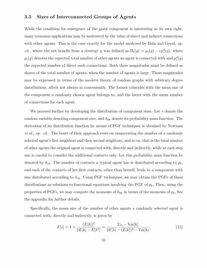
Specifically, the mean size of the number of other agents a randomly selected agent is
connected with, directly and indirectly, is given by
E[s] = 1 +(E[k])2
2E[k]− E[k2]=
2z1 − Var[k]
2E[k]− (E[k])2 − Var[k]. (15)
31
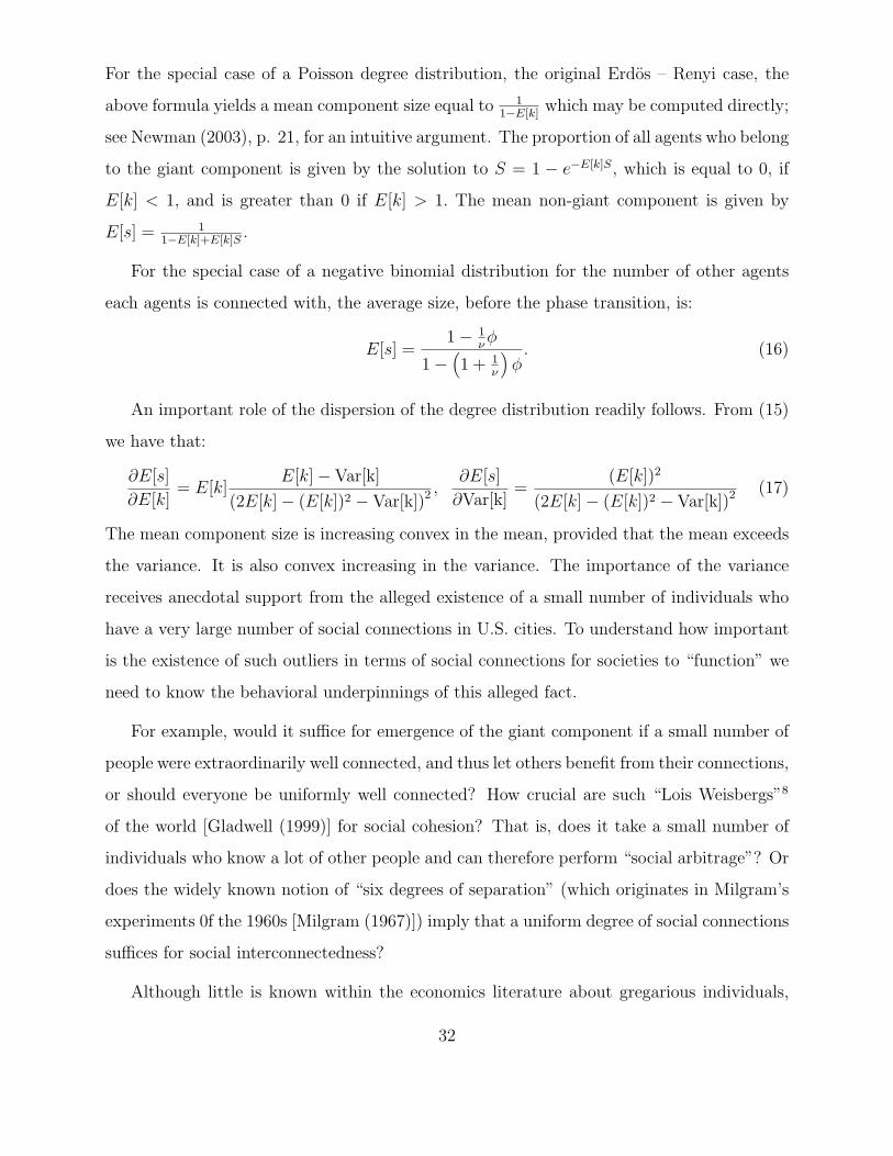
For the special case of a Poisson degree distribution, the original Erdos – Renyi case, the
above formula yields a mean component size equal to 11−E[k]
which may be computed directly;
see Newman (2003), p. 21, for an intuitive argument. The proportion of all agents who belong
to the giant component is given by the solution to S = 1 − e−E[k]S, which is equal to 0, if
E[k] < 1, and is greater than 0 if E[k] > 1. The mean non-giant component is given by
E[s] = 11−E[k]+E[k]S
.
For the special case of a negative binomial distribution for the number of other agents
each agents is connected with, the average size, before the phase transition, is:
E[s] =1− 1
νϕ
1−(1 + 1
ν
)ϕ. (16)
An important role of the dispersion of the degree distribution readily follows. From (15)
we have that:
∂E[s]
∂E[k]= E[k]
E[k]− Var[k]
(2E[k]− (E[k])2 − Var[k])2,
∂E[s]
∂Var[k]=
(E[k])2
(2E[k]− (E[k])2 − Var[k])2(17)
The mean component size is increasing convex in the mean, provided that the mean exceeds
the variance. It is also convex increasing in the variance. The importance of the variance
receives anecdotal support from the alleged existence of a small number of individuals who
have a very large number of social connections in U.S. cities. To understand how important
is the existence of such outliers in terms of social connections for societies to “function” we
need to know the behavioral underpinnings of this alleged fact.
For example, would it suffice for emergence of the giant component if a small number of
people were extraordinarily well connected, and thus let others benefit from their connections,
or should everyone be uniformly well connected? How crucial are such “Lois Weisbergs”8
of the world [Gladwell (1999)] for social cohesion? That is, does it take a small number of
individuals who know a lot of other people and can therefore perform “social arbitrage”? Or
does the widely known notion of “six degrees of separation” (which originates in Milgram’s
experiments 0f the 1960s [Milgram (1967)]) imply that a uniform degree of social connections
suffices for social interconnectedness?
Although little is known within the economics literature about gregarious individuals,
32

a few studies provide glimpses into the role of gregarious individuals as workers. Krueger
and Schkade (2005) document a positive and statistically significant relationship between a
worker’s tendency to interact with others (particularly with friends) while not working and
the relative frequency of worker-related interactions on the worker’s jobs. They interpret that
as evidence of sorting of more extroverted workers into more sociable jobs. The relationship of
remuneration to sociability, while controlling cognitive characteristics is also very interesting
but does not seem to have been addressed.
While our analysis so far has emphasized the mean component size, we may explore sev-
eral applications where agents’ benefits depend not only on expectations but more generally
on the actual distribution of component sizes. The moments of the distribution of compo-
nent sizes below and above the phase transition may be obtained. This is made possible by
working with PGF of the distribution of component sizes. The proportion of all agents that
are interconnected above the phase transition may be obtained, albeit not in closed form. It
may also be obtained numerically.
An interesting application would be to consider the following. Agents may randomly
become unavailable to interact with others, even though they may be connected with other
agents. Alternatively, consider that ideas or information arrive randomly at agents, and each
of them passes it on to each of her acquaintances with probability q. The expected number
of others who hear of the idea from an agent who has just received it and has degree k is
equal to q(k− 1). If agents fail to pass on the idea, then their neighbors who were connected
previously through them become disconnected from one another. The likelihood that an
individual receives the idea is proportional to her degree. Therefore, the average number of
other persons a person passes the idea on to is equal to: q∑
iki(ki−1)∑
iki
= q (E[k])2−E[k]E[k]
. More
formally, working from Newman (2002a) in the case of network resilience [ see the Appendix
for some further details ], we have that there exists a threshold value of the probability that
an agent is available, which is given by E[k]
Var[k]+(E[k])2−E[k].
For the special case of the negative binomial degree distribution examined above, this
threshold probability is given by: ν(ν+1)ϕ
. Not surprisingly, the stronger the “intensity” with
which the giant component would emerge, the higher the threshold probability. In other
33

words, indirect connections among agents make up for failure of individual agents.
3.6 Trade in Differentiated Products
This example motivates the model of the previous section via trade in differentiated com-
modities. Although not strictly necessary, it also employs a directed graph version of the
model, whereby a country (site) may sell to other countries and use the proceeds to pay in
turn for its own imports. Please see the Appendix for an elementary treatment of the case
of directed graphs.
Individuals in opening up connections with others are motivated by the desirability of
trade. We model the contacts among agents by means of directed graphs. Each agent may
be connected with others and other agents may be connected with her. A directed graph
accommodates conveniently a setting where an individual sells to those she is connected
with, her “out-edges,” and buys from those who are connected with her, her “in-edges.”
A particularly simple way to motivate such trade is by means of trade in differentiated
goods. Product variety is desirable and therefore motivates trade. Assuming monopolistic
competition, each differentiated good’s price is a constant mark-up of the wage rate, the
quantity of each variety produced at the free-entry equilibrium is constant and shared among
all agents and the market clears through the number of varieties. Therefore, an individual’s
welfare depends on the number of her contacts. This is why the model of differentiated goods
In order for an agent to acquire connections with others she has to incur costs. We simplify
the cost side by assuming iceberg costs.
Suppose that each site i is home to ℓ workers. A large number of firms may produce
any arbitrary number of varieties of a differentiated consumption good under conditions of
monopolistic competition using only labor, which the single undifferentiated input in the
world economy. There exists a universal unit of account, which may be used for settling
all transactions across sites. For simplicity, we make the additional assumption that there
is free entry, so that the number of varieties produced is determined and under symmetry
equal through all sites. We develop the formal dependence of the value from trade on the
34
number of trading partners.
We start the analysis by assuming that links between sites (that is, countries) are directed.
For each site, there exist in-connections and out-connections. The agents who are located
in site i may buy differentiated varieties from all other sites that are in-connected with site
i. Let nji+ denote the number of varieties imported into i from site j, and Ni+ =∑Jj=1 n
ji+,
denote the total number of differentiated varieties imported from all J other sites which have
in-connections with site i. Similarly, let nki−, denotes the number of differentiated varieties
exported to k from site i, and Ni− =∑Kk=1 n
ki−, denote the total number of varieties exported
to all K other sites with which site i has out-connections; and Ni denotes the number of
varieties produced in site i. Each site functions as an open economy by selling some of the
own-produced varieties of the differentiated good to the sites that are its out-connections
and uses the revenue thus generated to purchase varieties from the in-connections.
It is a well known result from international trade theory with differentiated products [
Helpman and Krugman (1985) ] that if wage rates are equalized across all sites, wi = w, then
the monopolistic competition pricing rule implies that prices would be equal across all sites.
Then the share of a typical agent’s expenditure on goods from site j is given bynji+
ni+Ni+. It
follows that the total expenditure on all imports by agents in site i is given by wℓ Ni+
ni+Ni+.
Applying the same logic to site i’s exports, we have that the share of expenditure on
varieties produced in node i by agents in node k that has an in-connection from node i
is given by Ni
Nk+Nk+. This in turn implies that the total expenditure by all sites that have
in-connections from site i on varieties produced in node i, that is, the total exports of node
i, are given by wℓ Ni∑Kk=1
1Nk+Nk+
. Thus, the condition for trade balance is that for a node
i total imports must equal total exports:
Ni+
ni +Ni+
= niK∑k=1
1
nk +Nk+
. (18)
Free entry in each site ensures that each variety is produced at quantity κζξ(1−ζ ), which
implies in turn that the number of varieties produced in each site are equal to ni = ℓ1−ζκζ
≡ n.
Thus, all sites produce the same number of varieties. The trade balance condition then
35

becomes: J1+J
= K1+K
, which implies:
J = K, (19)
that is, the number of in-edges and out-edges must be equal. Of course, this condition
cannot hold with probability 1, when connections are stochastic. Still, with a large number
of agents, it could be proven that condition (54) is sufficient to ensure that trade balance is
satisfied almost surely: z = EJ = EK. So, we conclude that at least for the purpose of
a symmetric model it suffices to work with an undirected graph.
There is potentially a large number of goods, which enter symmetrically into preferences.
Let all individuals have identical preferences, given by U =(∑
m cζm
) 1ζ , 0 < ζ < 1, where m
ranges over varieties available for purchase in the site where an individual is located. The
range is affected by trade and will be discussed further below. All goods are produced with
the same cost (labor requirements) function, which includes a fixed cost κ and a marginal
cost ξ, both defined in terms of units of labor. It is convenient to define σ ≡ 11−ζ , the
elasticity of substitution among the differentiated inputs.
Applying standard results from trade theory under monopolistic competition [ Helpman
and Krugman (1985) ], we have that if wi denotes the wage rate in site i, then profit maximiz-
ing by firms under conditions of free entry implies a price which is constant for all varieties
produced in site i and equal to pi =ξζwi. An individual who is located in site i has demand
for a particular differentiated variety m given by:
cdm = wip−σm
P−(σ−1)i
,
where Pi =(∑
m (pm)1−σ
) 11−σ denotes the price index for all goods available in site i, each
of which are indexed by m. Note that the price elasticity of demand for each of the differen-
tiated goods is equal to minus the elasticity of substitution among differentiated products,
σ. Furthermore, it is a standard feature of this theory that the smaller is σ, the higher the
market power of each firm. In the limit when σ tends to infinity, the model of monopolistic
competition implies perfect competition.
To see the basic workings of this model, consider how expenditure is allocated to different
varieties of goods. First, we note that all goods produced in a site would be priced at the
36
same price. There are ni goods produced in site i and nji+ are imported from site j to site
i. Therefore, the price index in site i may be written as:
Pi =
Nip1−σi +
J∑j=1
nji+p1−σj
11−σ
. (20)
If wage rates were equalized across all sites, wi = w, then the pricing rule implies that prices
would also be equal across all sites.
If creation of connections between sites is up to individuals’ initiative, then individuals
have an incentive to spend resources in the creation of additional connections because doing
so increases the number of varieties they may purchase from n, under autarky, to n + nJ,
if they may purchase from J other sites as well, that is when site i is connected with J
other sites. Using the behavioral model for individuals above, we have that the indirect
utility function is Uaut = ζξ
ζn
1ζ−1. If J sites have in-connections with site i, then indirect
utility conditional on the number of in-connections being equal to J becomes U(J) = (1 +
J)1ζ−1Uaut. This quantity is random but always larger than under autarky, when J > 0,
and therefore so is its expected value. That is, if the actual number of in-connections is not
known when decisions about contacts are made, then an agent’s expected welfare is measured
as her expected utility, that is, the expectation of U(J) with respect to J . To motivate a
genuine tradeoff, it must be the case that there is a cost associated with the expansion of
the variety of goods associated with creating connections, such as transportation costs for
the imported goods. In that case, an increase in the variety of goods improves welfare but
comes at the cost of increased import prices.
We see this tradeoff clearly by letting transportation costs be in the form of iceberg costs:
to have a unit of a good from site j available in site i, eτ units of the good must be purchase
in site j, where τ, τ > 0, is a parameter. So, the c.i.f. price in site i of a differentiated good
produced in site j is pjeτ , and therefore the price index when differentiated varieties may be
imported changes from (20) to become
Pi =
nip1−σi +J∑j=1
nji+p1−σj e(1−σ)τ
11−σ
.
Indirect utility, conditional on the number of in-connections being equal to J, is given by
37

U(J) = ζξn
1σ−1
(1 + Je(1−σ)τ
) 1σ−1 , is a decreasing function of transport costs, cet. par.,
which makes intuitive sense. Therefore, while more connections , with other sites, more
varieties may be imported leading to greater welfare. However, the welfare enhancing effect
of additional in-connections is dampened by the impact of transport costs.
Let E[k] and Var[k] denote the mean of variance of the degree distribution. Expected
indirect utility may be written as:
EU(J) = Uaut(1 + E[k]e(1−σ)τ
) 1σ−1
[1− 1
σ − 1
(1− 1
σ − 1
)Var[k]
(e(σ−1)τ + E[k])2
]. (21)
We note that the impact of uncertainty in the number of connections depends on the actual
magnitude of the elasticity of substitution. If σ is larger (smaller) than 2, then the indirect
utility function is concave (convex) in the number of connections with other sites, and the
increased varieties made possible by the degree distribution decreases (increases) welfare.
If the mean and variance of the number of connections may vary independently — as
in the case of a negative binomial distribution that we examined earlier —, then for given
values of E[k] and τ, (21) implies that there exists a threshold value of Var[k], above which it
is not attractive to an agent to invest in connections. That is, for the presence of connections
to pay, it must be the case that
2E[k]−(E[k2]
)2≤ Var[k] ≤ σ − 2
(σ − 1)2
1− eτ
(e(σ−1)τ + E[k])1
σ−1
(e(σ−1)τ + E[k])2. (22)
We note that in view of (12), Var[k] must exceed 2E[k] − (E[k])2. Therefore, for both the
condition for phase transition to hold and for connections to be attractive, the relationship
between the mean and the variance is restricted.
Transport costs have a subtle effect. They reduce welfare because they increase costs, but
their dampening of the welfare-enhancing effect of greater variety also reduce its variance.
3.7 Graphical Economies: Extension of the Arrow–Debreu Model
In one of the most interesting recent developments of research on economies embedded in
graph settings, economists and computer scientists have examined economic transactions
38

of various kinds, ranging from exchange to auctions. These new works provide important
motivation for economic interactions among agents, in contrast to much of the social networks
literature where agents are typically assumed to be passive.
Kakade et al. (2004a, 2004b) have sought to extend the range of key results in math-
ematical economics, such as the Arrow–Debreu theorem on the existence of competitive
equilibrium [ Arrow and Debreu (1954) ], to “graphical” economies. They define graphical
economies in terms of a given graph topology, G, of what direct trades are allowed among
individuals. In the setting of Kakade et al. (2004a) there exist i = 1, . . . , I individuals and
j = 1, . . . , K physically different goods. Goods are indexed by their sellers, so that there is a
total of I ·K goods. The same physical goods sold by different sellers are perfect substitutes.
An undirected graph over I defines trade restrictions; lack of an edge i′, i′′ means that
those two individuals may not trade directly with another. In other words, every consumer
is allowed to buy goods only from her neighbors, ν(i), that is xij = 0, j ∋ ν(i), and market
clearing is local: each individual’s value of supply (endowment) vector is equal to the value
of her demand vector at the “local” prices.
Let pik be the price of good k sold by individual i. The vector of prices of all goods
sold by an agent define to local price vector, pi. Individual i’s consumption plan satisfies∑j∈ν(i) p
j · xij = pi · ei, where ei denotes her endowment of goods. Proving existence of a
graphical equilibrium, that is existence of a set of prices, P = . . . ,pi, . . ., and plans in which
all plans are optimal at the prices and all markets for each agent i clear:∑j∈ν(i) x
ji = ei. This
requires an extension of the Arrow–Debreu model. That is, it is necessary to ensure that no
individuals are left with endowments valued at zero: there are in effect I ·K goods but each
individual has an endowment of K goods and is allowed to sell at the “local” prices only.
Existence of a graphical equilibrium amounts to existence of equilibrium price dispersion.
Graphical equilibria and Arrow-Debreu equilibria coincide if graph G is connected.9
Kakade et al. (2004b) apply this framework to examples where the graph, G of trade
restrictions is random. They use a bipartite random graph and compare bipartite versions
of the Erdos – Renyi model and of a random version of the preferential attachment model.
According to the latter, the economy starts with a buyer and a seller. At each subsequent
39
step an additional buyer and an additional seller are added: the buyer is connected with
probability α to a seller in the existing graph uniformly at random, and with probability
1 − α the buyer is connected to a seller in proportion to the existing degree of the seller.
Simultaneously, a seller is attached in a symmetric manner, with probability equal to α
randomly, and to 1 − α with preferential attachment. They also examine a modification
that allows a buyer to be connected to more than one sellers, a feature that produces trade
restriction graphs that are not just trees. All sellers sell only one and the same good.
Structural properties of G are reflected in price dispersion. It is known from the preferential
attachment literature, the resulting degree distribution can be approximated by a power law.
Therefore, an attractive interpretation of the model may be a model for the distribution
of wealth, in which case the preferential attachment model would predict a power law.
In contrast, for the Erdos – Renyi model with a large number of agents and a constant
probability for each edge, price dispersion takes a very different form.10 This particular
application by these authors suggests that it would be interesting to examine the contribution
of “connection” uncertainty (how many other traders a trader trades with) as separate from
endowment and price uncertainty to the distributions of such outcomes as income and wealth.
See also Ioannides and Loury (2004). Of particular interest is to examine the origin of the
sensitivity of outcomes to parameter values, which was discussed in section 2 above.
3.7.1 Other Models of Interactions with Direct Neighbors
The literature has considered also problems set in networks that are populated by agents who
value interactions with their direct neighbors, and whose objectives therefore involve mea-
sures based on the number of direct connections. Consider a setting like that of Bramoulle
and Kranton (2003), where agents value the private information they receive from their
immediate (first) neighbors. So individual i values the total information in his posses-
sion, ei +∑j∈ν(i) ej, and incurs a constant marginal cost c. That is, agent i’s payoff is
U(e,G) = b(ei +∑j∈ν(i) ej) − cei, where G denotes social structure, ν(i) denotes agent i’s
neighborhood, and the function b(e), with b(0) = 0, is increasing and concave in its argu-
ment. An individual benefits from the sum total of the information directly possessed by
40

her neighbors and in turn her own information benefits her neighbors. Depending upon as-
sumptions made about the social structure, an agent’s neighborhood may be either fixed or
random. This model may accommodate the case where the benefits derive from locating the
lowest price seller among a number of sellers. Other literature has interpreted direct connec-
tions themselves as a measure of social capital. This is the case with one of the models in
Mobius and Rosenblat (2002), where if an agent’s neighbor is unable to provide a favor, she
in turn appeals to one of her own other connections. A particularly interesting consequence
of valuing direct contacts only is when agents’ behavior brings about the emergence of the
giant component in the social network.
3.8 Social Networks versus Other Networks
The recent econophysics literature recognized that models that have been proposed to study
engineering and biological networks do not perform well when it comes to social networks.
As Newman and Park (2003) underscore, social networks exhibit non-trivial clustering, or
network transitivity, and show assortative mixing, that is positive correlation between the
degrees of adjacent nodes. Empirically speaking, most other networks show disassortative
mixing. These authors suggest that the community structure of social networks may explain
both clustering and assortative mixing, which do not vanish as the size of the network
increases. If individuals who belong to small groups tend to have few connections and are
connected to others in the same group, who are also like themselves, and similarly individuals
who belong to large groups tend to have more connections and are connected to others in the
same group, then variation in the size of groups would produce assortative mixing. Newman
and Park obtain rigorous results on the impact of community structure in social networks
by describing (through its PGF) the joint probability distribution for ejk, the number of
“excess” nodes that a randomly chosen edge is connected with, that is the number of other
edges attached to the node other than the one that is randomly selected. This allows them
to write an expression for the assortativity coefficient, the excess correlation coefficient for
41

the number other nodes each edge is connected with,
r =1
σ2q
∑jk
jk(ejk − qjqk), (23)
where qj denotes the probability distribution for excess degrees for a randomly selected
neighbor, qj =(k+1)pk+1∑
kkpk
, and σ2q its variance. They show that given p, the probability that
individuals are acquainted with one another, the probability functions for rm, the number of
groups each individual belongs to, and for sn, the size of groups, the assortativity coefficient
is positive. In the special case when both the number of groups and the sizes of groups have
Poisson distributions with parameters µ and ν respectively, then the assortativity coefficient
is given by: r = p1+µ+νµp
. As either of the two means µ and ν increases, the assortativity
coefficient decreases. This is straightforward when it comes to increase of the mean number
of groups an individual belongs to: the more groups an individual belongs to, the less the
relative within-group correlation upon which assortativity depends. That is, the within-
group correlation is diluted by all the other groups the individual belongs to. Increase
in mean group size also increases dispersion, and therefore fewer individuals with similar
numbers of connections will fall within the same community.
Detecting community structure in networks, which is essential in understanding the struc-
ture of networks, is a hard computational problem. See Newman (2004) for a review of
different approaches. Essentially, the statistical inference problem by means of a standard
method like maximum likelihood estimation is complicated by the fact that a large number
of possible configurations must be considered, whose number increases exponentially.
Recently, Copic, Jackson, and Kirman (2005) get additional mileage by motivating an
abstract problem of community structure as a problem of identifying communities of scientific
journals in terms of patterns of cross-citations. They axiomatize their approach by means
of ranking partitions of a graph in terms of likelihood. Specifically, let Π(I) be the set of all
partitions of I nodes, π its generic element, and for any i ∈ I, let cπ(i) be the component of π
containing i. A community structure is a partition of I. Any two nodes within a community
“interact,” are connected, with probability pin, and any two nodes from different communities
“interact,” are connected, with probability pout. Their model allows for multiple interactions
42
sij between any two nodes i, j. So, the likelihood of seeing gij out of sij is:
pgijin (1− pin)
sij−gij ,
if i, j belong to the same community, and
pgijout(1− pout)
sij−gij ,
if i, j belong to different communities. The likelihood of observing any given pattern of
cross-citations is given by:
Ls,g(π) =∏i∈I
∏j∈cπ(i)
(pin)gij(1− pin)
sij−gij
∏j∈I\cπ(i)
(pout)gij(1− pout)
sij−gij
. (24)
Any two community patterns may be compared in terms of their likelihood, and their max-
imum likelihood provides an ordering of all partitions on Π(I). They apply their method to
data on cross-citations among economics journal in 1995–1997 and estimate a pair of proba-
bilities (pin, pout). Of course, the world is more heterogeneous and, in particular, hierarchical.
A lot of people publishing in journals that cite the American Economic Review frequently
are not necessarily themselves cited by author publishing in the American Economic Review.
While detecting community structures has generated scientific interest, there is also con-
siderable interest within business. Recent business ventures are notable for exploring “re-
lationship capital.” One such company, Visible Path, promises to use the “the Science of
Trust” to “transform the way large companies leverage relationship capital to drive top line
revenue growth” [www.visiblepath.com].
3.9 Centrality and Searchability of Random Graphs
Another aspect of social structures that are modelled as random graphs is centrality. This
is a core sociological concept [ Wasserman and Faust (1994) ], that has received renewed
attention in the Internet era. Is there a sense in which we may characterize each individual
in terms of her social importance? If connections confer social importance, then let the
importance of agent i be ϖi, and let us assume that this is proportional to the sum of the
43

importance of the other agents she is connected with. That is: ϖi = λ−1∑j Γijϖj. By
rewriting this in matrix form with ϖ an I−vector denoting social importance of respective
agents, we have:
Γϖ = λϖ. (25)
In other words, the vector of individuals’ social importance, ϖ, and the respective coeffi-
cient of proportionality, λ, are an eigenvector and its respective eigenvalue of the adjacency
matrix Γ. Since the adjacency matrix is symmetric and positive, the Perron-Frobenius theo-
rem guarantees the existence of a maximal positive eigenvalue and a corresponding positive
eigenvector, provided that the graph is connected, or else the maximal eigenvalue would be
equal to zero [ Cvetkovic et al. (1995) ]. If the social structure is not known with certainty
and may be described by a random graph, what can we say about centrality of the resulting
graph?
While the centrality of the resulting random graph is hard to characterize, the associated
eigenvalue, the inverse of the coefficient of proportionality, is much easier. It is well known
that the maximal eigenvalue is contained between a graph’s maximal degree and its average
degree [ Cvetkovic et al. (1995) ]. For a random Erdos – Renyi graph corresponding to a
constant edge probability p, its maximal eigenvalue is asymptotically normally distributed
with mean (I − 1)p + (1 − p) and variance 2p(1 − p). Therefore, the maximal eigenvalue
increases linearly with the number of agents. When the edge probability decreases as the
number of agents increases as p(n) = O(ℓnn), the case of the sparse random graph, the largest
eigenvalue is given by (1+ o(1))max√∆, Ip, where o(1) tends to 0 as max
√∆, Ip tends
to infinity and ∆ is the maximum degree of the graph [ Krivelevich and Sudakov (2003) ].
The asymptotic behavior of the largest eigenvalue is quite critical to network search because
the associated eigenvector gives the social importance of different sites. In fact, some of the
latest developments in the literature on the searchability of the web depends on topological
characteristics of the random graph. For example, the popular search engine Google employs
a variation of the above network centrality model in arriving at a ranking for the importance
of web sites [Newman (2003d)].
44

3.10 Applications with Models of Job Matching
The job search model addresses the problem of matching workers and firms. This is an
inherently discrete problem and therefore its stochastic versions have been typically handled
by means of Poisson models or models of other point processes [ Pissarides (2001) ]. The
underlying discrete assignment problem has itself received attention; see Akerlof (1981) and
Shimer (2003), most recently. We examine next a multilateral job matching model, where
agents contact several agents on the other side of the market.
Let the sets denoting firms and workers (with each firm being a “job,” employing one
worker) be, respectively: M = 1, 2, . . . ,M, N = 1, 2, . . . , N. Let pj denote the prob-
ability mass function for the random variable J that denotes the number of different firms
that a worker is connected with. Under the assumption that there is at most one connection
with each firm, J may take values j = 1, . . . ,M. Let f0(x) be the PGF of pj. Let qk denote
the probability mass function for the random variable K that denotes the number of different
workers that a firm is connected with. Under the assumption that each firm has at most one
connection with each worker, K may take values k = 1, . . . , N. Let g0(x) be the PGF of qk.
The means of the respective distributions are denoted by, respectively: µ = f ′0(1), the mean
number of firms a worker is in contact with, and ν = g′0(1), the mean number of workers a
firm is in contact with. For consistency, it should be the case that Mν = Nµ.
If workers are matched with firms at the workers’ sole initiative, the two distributions
pj, qk, may not specified arbitrarily; in fact, in that case, the probability mass function qk is
derived from pj. This is, of course, well recognized and easily derived in models of job search
where individuals apply to only one job at a time. Yet, the derivation in case of multilateral
matching is quite complicated [ Albrecht et al. (2003) ].
Worker and job matching may be modelled as a bipartite graph, with the two respective
groups of nodes being the sets of firms and of workers, M and N , respectively. Next we
consider the groups of all workers who are in contact with the same firms. Individuals
who have been in contact with the same firm may be affected similarly in a variety of ways,
including most notably the fact that only of them would be chosen for employment. Similarly,
45

sets of firms who are in contact with the same individuals may be impacted in similar ways.
We can derive the probability generating functions (and through them the parameters of the
respective mass functions) for these groups of workers and separately, of firms.
Consider a contact between a firm and a worker that is chosen randomly from among
all such contacts, that is, from among the edges of the bipartite graph describing such
connections. Now, consider the respective firm and worker linked by such a contact. Let
the PGF of the distribution of the number of other firms that a worker thus chosen is also
in contact with be f1(x), and of the number of other workers that a firm thus chosen has
established contact with be g1(x). From Newman et al. (2001), p. 11, these PGFs are given
by, respectively:
f1(x) =1
µf ′0(x), g1(x) =
1
νg′0(x). (26)
Again, these distributions reflect the impact of connection-biased sampling.
Consider the distribution function of the number of other workers who are in contact with
the same firms as a randomly chosen worker. These workers share in common information
about the same firms. Its PGF is given by: G0(x) = f0(g1(x)), [ ibid. ]. That is, this is
the PGF for the degree distribution for a graph defined as having as nodes all workers and
edges connecting pairs of workers who are in contact with the same firms. In graph-theoretic
terms, this is the distribution of the number of first neighbors, when two workers are assumed
to be neighbors if they are in contact with the same firm. Working in like manner, for a
randomly chosen contact between a firm and a worker, consider the worker thus chosen:
the distribution of the number of other workers that are in contact with the same firm as a
worker thus chosen is given by: G1(x) = f1(g1(x)). Working for the number of firms who are
in contact with the same worker, that is, the PGF for the degree distribution for a graph
defined as having as nodes all firms and edges connecting pairs of firms who are in contact
with the same workers. Its PGF is given by: F0(x) = g0(f1(x)),
To give an example, consider that the number of firms each worker has a contact with
has a Poisson distribution with parameter µ, and that the number of workers each firm
has contacts with has a Poisson distribution with parameter ν. Thus f0(x) = eµ(x−1) =
f1(x), g0(x) = eν(x−1) = g1(x). The PGF for the distribution function of the number of other
46
workers who are in contact with same firm as a randomly chosen worker is G0(x) = G1(x) =
e[µ(eν(x−1)−1)]. The PGF for the distribution function of the number of other firms who are in
contact with same worker as a randomly chosen firm is F0(x) = F1(x) = e[ν(eµ(x−1)−1)]. The
average number of first neighbors, the average number of other workers that are in contact
with the firms with which a worker is also in contact, is given G′0(1) = µν. The average
number of second neighbors is: ddxG0(G1(x))
∣∣∣x=1
= G′0(1)G
′1(1) = f ′
0(1)f′1(1)[g
′(1)]2 = (µν)2.
The second moment of G0(x) is given by(x ddx
)2G0(x)
∣∣∣∣x=1
= µν[1 + ν + µν]. The second
moment of F0(x) is given by(x ddx
)2F0(x)
∣∣∣∣x=1
= µν[1 + µ + µν]. Finally, the condition for
emergence of the giant component in the graph of workers who have been in contact with the
same firm is ν ≥ 11+µ
, and the condition for emergence of the giant component in the graph
of firms who have been in contact with the same worker is µ ≥ 11+ν
. It would be interesting
to apply this model to the case of assignment of workers to jobs in presence of coordination
frictions in the style of Shimer (2003).
4 Markov Random Graph Models of Social Interac-
tions
While interest in social networks is relatively recent within economics, the subject has at-
tracted continuous interest in mathematical sociology. We seek to draw lessons by con-
trasting the economics, econophysics and mathematical sociology literatures. A landmark
development in the mathematical sociology literature is a number of models dating back to
Holland and Leinhardt (1977) that characterize the evolution of the entire social structure
as a stochastic process. A common problem faced by these approaches is how to model in a
tractable way the possible dependence between the decisions of different agents and between
decisions made by a single agent in contacting other agents. For example, the original model
of Holland and Leinhardt rests on the assumption that the states of different agents, given the
state of the social structure in the previous period, are conditionally independent. A great
potential that has been opened up by the economics literature is exactly in offering predic-
tions about the properties of the entire network that follows the development of contacts by
47
individual agents. Furthermore, a key aspect of the description of random graphs by means
of arbitrary degree distributions is that it is no longer possible to consider the probability
of individual links as a building block of the model. Therefore, the modern literature on
random graphs has addressed successfully the problem of generalizing the degree distribution
but not transitivity, the phenomenon whereby the acquaintances of my acquaintances are
also likely to be my acquaintances, too. But the techniques developed by the newer literature
on random graphs with arbitrary degree distributions rests heavily on the assumption of the
numbers of connections in adjacent nodes being independent. The usefulness of the network
formation models extends to allowing us to consider the simultaneity of individual decisions.
With an eye on this objective, we discuss next a particular approach to the study of so-
cial networks that allow for dependence among graph-related attributes of connected nodes.
Except for some special cases, this appears to be the only approach that allows modelling
transitivity of social connections. Following Newman (2003), p. 26, any measurable proper-
ties of a graph, ϵi, such the number of edges, the number of vertices of a given degree, or
the number of triangles, may be associated with an exponential random graph model. That
is, the probability of a graph G is given by
Prob(G) =1
Ze−∑
iβiϵi , Z =
∑G
e−∑
iβiϵi , (27)
where Z denotes the partition function. In calculating all of the possible realizations, we
would take into consideration the specifics of the problem. This approach may in principle
be applied to any problem. Unfortunately, only very special problems may lend themselves
to analytical derivations that allow one to study the behavior of these models as parameters
change.
Fortunately, an interesting benchmark is available in the form of the so-called “2-star”
model of a network, that is the case when the network may exhibit only pairs of edges that
share a node, Park and Newman (2004a) have obtained an analytical solution. The 2-star
model follows from (27) in the special case when
Prob(G) =1
Zexp
[− J
I − 1
∑i
k2i −B∑i
ki
], (28)
where ki denotes the degree of vertex i. The solution involves the parameters B, J, I of
48
the model and ϕ0, which is defined as the solution to ϕ0 = 12[tanh(2Jϕ0 + B) + 1]. In the
approximate mean-field case, E[k] = (I − 1)ϕ0 and a variety of properties of the random
graph, the actual mean degree, the mean squared degree, etc., may be expressed in closed-
form in terms of B, J, I and of ϕ0 [ ibid., p. 3 ]. Those expressions are complicated functions
of the basic parameters, in addition to ϕ0. Specifically, the mean, the mean squared and the
variance of the degree distribution are given by:
E[k] = (I − 1)ϕ0 +2Jϕ0(1− ϕ0)(1− 2ϕ0)
(1− 4Jϕ0(1− ϕ0)) (1− 2Jϕ0(1− ϕ0)), (29)
E[k2] = (I − 1)2ϕ20 +
(I − 1)ϕ0(1− ϕ0)(1− 4Jϕ20)
(1− 4Jϕ0(1− ϕ0)) (1− 2Jϕ0(1− ϕ0)), (30)
E[k2]− (E[k])2 = (n− 1)ϕ0(1− ϕ0)
(1− 2Jϕ0(1− ϕ0)). (31)
This helps make clear that the “deep” parameters of the Markov random graph model would
generally be hard to recover in an estimation setting. The “silver lining” is that one may
check directly whether the underlying network possesses a giant component, that is under
what conditions on the parameters of the model E[k2] ≥ 2E[k].
4.1 The Frank–Strauss Model of Markov Random Graphs
Although this approach may accommodate different measurable properties of graphs, we
stick to graph topology in this exposition. We describe a social network G in terms of
its adjacency matrix as a random matrix. As suggested by Frank and Strauss (1986) and
Strauss (1986), the dependence structure among the random variables describing connections
between different agents are described by the dependence graph D of the random matrix
Γ. The dependence graph is a non-random graph that specifies the dependence structure
between the(I2
)random variables γij that denote all possible connections among individual
agents. The nodes of D are the element of the index set (i, j); i, j,∈ I, i = j, that is all
possible edges of G. The edges of D signify pairs of the random variables that are assumed
to be conditionally dependent, given the values of all other random variables. That is, D
has an edge between (i, j) and (k, ℓ), if γij and γk,ℓ are conditionally dependent.
49

Frank and Strauss (1986)11 invoke the Hammersley–Clifford theorem [ Besag (1974) ]
and obtain a characterization of the probability function for the realization of a random
undirected graph Γ, with dependence graph D. This probability is given by
Prob(Γ) = c−1 exp
[∑A⊂Γ
αA
], (32)
where αA is an arbitrary constant, if A is a clique of D, αA = 0, otherwise; c is a normalizing
constant. If the maximal cliques of D are disjoint, then it follows that a general probability
distribution of Γ is specified by separate probability distributions of the maximal sufficient
subgraphs of Γ. Because of the exponential expressions involved in describing this model,
which originate in the Markov random field expressions associated with the Hammersley–
Clifford theorem, these class of models are known as exponential random graph models.
To see the power of the theorem, let us consider a Bernoulli graph, that is, a random
graph where all edge indicators γij are mutually independent Bernoulli random variables,
with edge probabilities pij. Then,
Prob(Γ) =
∏(ij)∈Γ
exp[αij]
1 + exp[αij]
× ∏(ij)/∈Γ
1
1 + exp[αij]
, (33)
and pij = exp[αij ]
1+exp[αij ]. The Erdos–Renyi random graph follows for the special when all edge
probability are equal.
Frank and Strauss introduce the notion of a general Markov graph, as a graph whose
dependence graph has no edges between disjoint sets of nodes, such as (i, j) and (k, ℓ). That
is, for a Markov graph Γ, edges which are non-incident to the same node are conditionally
independent. That is, decisions about connections between different pairs of agents (j, k)
and (j′, k′) are independent, as long as j = j′ = k′ = k′. This implies readily that the cliques
of the dependence graph of a Markov random graph correspond to sets of edges such that
any pair of edges within the set must be incident. Such sets are just triangles and stars, that
is k−stars, k = 1, . . . , I − 1 [ ibid., p. 835 ]. This allows us to write a general expression for
the probability of any arbitrary undirected Markov graph:
Prob(Γ) = c−1 exp
[∑α(Tuvw) +
I−1∑k=1
∑ 1
k!α(Sv0...vk)
], (34)
50

where the first sum enumerates and sums up over all(I3
)distinct triangles, Tuvw, Tuvw ⊂ Γ,
the second sum enumerates and sums up over all distinct k−stars, for k = 1, . . . , I − 1, and
the functions α are vectors of parameters.
This results admits two simplifications. First, under an assumption of homogeneity,
namely when all topologically isomorphic graphs have the same probability, the argument
of exp[·] above is simplified to: αtt+∑I−1k=1 αksk, where t is the number of triangles in Γ and
sk the number of k−stars in Γ, and αt, αk are parameters. Homogeneity essentially means
that nodes, that is agents, are a priori indistinguishable and therefore only distinct graph
topologies matters. Second, in view of the fact that the k−star specific parameters in (34)
are hard to interpret, because every k−star contains
(kj
)j− stars as well, j < k, Frank
and Strauss, ibid., p. 836, show that the probability of a general homogeneous graph is
equivalently rewritten in terms parameters corresponding to the degree distribution of graph
Γ as:
Prob(Γ) = c−1 exp
αtt+ I−1∑j=1
αjdj
, (35)
where dj denotes the number of vertices of degree j in Γ. This is the probability of graph Γ,
conditional on the number of triangles t, and on the number of nodes with different degrees.
Some remarks are in order. First, we note that the above expressions give probabilities for
events defined as realizations of entire graphs. Therefore, they are appropriate to consider
when we know the outcome of individual decisions that satisfy the conditions that define
Markov graphs. That is, for a model where individuals make individual decisions to contact
others, and the decisions to each individual makes to contact all others are statistically
dependent, then (35) gives the probability that a graph with t triangles and dj, j−stars
j = 1, . . . , I − 1, will be realized.
Park and Newman (2004c) obtain exact (though not closed-form) solutions for the pa-
rameters of a special case of the above model, that is for an exponential random graph, for
which a graph with a total number of edges and of triangles, denoted by D(Γ) and t(Γ), re-
spectively, occurs with probability proportional to e−[αdD(Γ)−αtt(Γ)]. Let p = E[γij] denote the
probability ( connectance ) that the typical edge is present, q = E[γijγjk] and the probability
51
of a two-star (or dyad), and r = E[γijγjkγki] the probability of a triangle, in exponential
random graphs with a probability being proportional to e−[αdD(Γ)−αtt(Γ)]. Using tools from
Park and Newman (2004b), they show that q, the expected number of dyads, is given by the
solution of
q =eαd−αt(I−2)q + eαt
(eαd−αt(I−3)q + 1)2(eαd−αt(I−2)q + 1) + (eαt − 1)
, (36)
and the expected number of triangles in the graph is given by:
r =eαt
(eαd−αt(I−2)q + 1)3+ (eαt − 1)
. (37)
The RHS of Equ. (36) is monotone increasing in q, but may, depending upon parameter
values, be sigmoid and have either three fixed points or one fixed point. The former, the
“broken-symmetry” case, is associated with two areas of parameter values for which the
density of triangles is high and low. The latter, the symmetric case, is associated with
coexistence of both high and low density areas of triangles. While these derivations are for
the so-called mean field case, these authors show that they are exact in the case of large
number of agents.
Second, this is an equilibrium outcome that follows from the theory of Markov random
fields and is consistent, in principle, with a variety of individual contact processes, but is not
linked to any specific law of individual decision making. It is derived under the assumption
of a finite number of agents. Presumably, taking limits for large numbers of agents may lead
to results similar to those of the random graph literature. However, this particular literature
has emphasized empirical applications, especially by sociologists, except for the papers by
Park and Newman, referred to above.
Third, with an eye to empirical applications, it needs to be stressed that estimations with
the Frank–Strauss model pose some problems, in that the normalizing constant contains
parameters that also appear in the numerator of the RHS of (35) and need to be treated as
nuisance parameters.
Fourth, Newman (2003) claims that the model is vulnerable to a particular property of
generating too many complete cliques. These contribute to the overall clustering coefficient
but generate unevenness across the graph.
52

Fifth, this approach has been quite popular for structuring estimation models associated
with different types of properties of graphs. See, in particular, Anderson, Wasserman and
Crouch (1999), Pattison and Robins (2002), Pattison and Wasserman (2002) and Wasserman
and Robins (2001), who discuss various aspects of the estimation problem. Finally, Morris
(2003) offers a more optimistic assessment of the prospects of applications of exponential
random graph models when the dependence can be thought of as a neighborhood effect.
5 Observable Consequences of Optimizing Behavior in
Networks
I conclude by looking at whether observable consequences of optimizing behavior may serve
as basis for empirical investigations. The modern literature on networks has emphasized
certain stylized facts, such as the degree distributions typically obeying power laws and
topological features conforming to certain predictions. The literature has addressed the
presence such stylized facts by means of models with large graphs. Yet, the empirics in this
area have not received sufficient scrutiny. When they did receive such scrutiny, as in the
case of Faloutsos et al. (1999) by Chen et al. (2002), the empirical case for power laws
considerably weakened, as we discuss below.
5.1 Actions as Outcomes from Games in Finite Networks
We take up the matter of observable consequences of optimizing behavior in networks by
considering first the case of finite graphs. When individuals interact with a finite number
of other individuals, it is natural to consider interdependence of their actions in the light
of game theory. Galeotti et al. (2006)12 offer a systematic framework for the treatment of
strategic interactions when the definition of neighborhood is described either in terms of
full knowledge of a network and other individuals’ positions in it, or of knowledge of the
network’s degree distribution, when the information is incomplete. Their models allow for a
general class of payoffs, which have as special cases practically all previously studied models,
53

and for incomplete information about network structures. Their results apply to interactions
between individuals and their immediate, that is direct, neighbors only. They depend crit-
ically upon whether different individuals’ actions are either complements or substitutes, or
are subject to positive or negative externalities from others. Generally, most of their results
assume that different individuals’ degrees are independent. Their results are derived under
the assumption that adding a link to a neighbor who chooses action 0 is payoff equivalent to
not having an additional neighbor. Consequently, their results do not apply to the case when
payoffs are sensitive to average actions of neighbors or to their product. Although the case
of dependence on the average action of neighbors is quite well understood from the social
interactions literature, it would be interesting if one could nest such dependence within the
general theory proposed by this paper.
5.2 Actions in Large Networks
Carlson and Doyle (1999) (see also Newman et al. (2002b)), introduce the concept of “highly
optimized tolerance” as a feature of either natural selection or deliberate engineering design
that provides robust performance in uncertain environments. They argue that the “ubiqui-
tous,” at least in the view of certain scholars, presence of power laws in various measures
associated with networks is indicative of individual optimization. As far as empirically pre-
dictions are concerned, there are very few papers that offer such predictions. Fabrikant et
al. (2002), discussed above, is the only paper that obtains power law distributions from a
model of individual optimization in certain graph measures arising in the Internet topology
precisely when new nodes that randomly appear choose optimally their connections with
an existing network. Barabasi and Albert (1999) also predict a power law for the degree
distribution of the web graph, but theirs is a reduced-form model of preferential attachment.
That is, a new edge is assumed to attach itself to an existing node of degree k in the network
with probability equal to kpk2E[k]
, where 2E[k] is the mean degree in the network. This implies
a degree distribution given by pk =2E[k](E[k]+1)k(k+1)(k+2)
. In the limit of large k this becomes propor-
tional to k−3, that is, it becomes a power law with exponent equal to 3. This can hardly be
a general case, of course.
54
The actual empirical research that made power laws prominent as explanations of the
degree distribution of the internet, such as Faloutsos et al. (1999), can easily be criticized,
and has in fact been severely criticized, on a variety of grounds even within the computer
science literature [ see, in particular, Chen et al. (2002) ]. However, the significance of the
findings lie in their having led the networks literature to direct attention to completely dif-
ferent dynamics than was the case before. Prior to these findings, the operating assumption
in the literature was that the Internet obeyed an Erdos – Renyi random graph!
However, as several authors have emphasized, including, in particular, Newman (2003)
and Dorogovtsev and Mendes (2003), different observed networks have sharply different fea-
tures. Therefore, it should be possible, in principle, to test different models of network
formation, that incorporate the specifics of different settings and thus have different impli-
cations in different circumstances. For example, certain kinds of social relationships require
more deliberate effort in order to be maintained than others. Therefore, going back to
behavioral routes is essential for understanding real world networks.
5.3 Implications for Behavioral Modelling
A particularly interesting area that has been revealed by the present essay is the need to
acknowledge the importance of the data generating mechanism when data on social networks
are used for the purpose of econometric analysis. Just as with length biased sampling in
studies with data on unemployed workers, data on individuals’ connections with others must
be treated differently, depending upon whether they have been collected from a random
sample of individuals or from a random sample of connections.
Suppose that we have information, possibly from micro data, on agents’ connections
with other agents. What can we infer about the property of social networks that may be
associated with these data? Is individual information on agents’ connections compatible
with existence of a network linking these agents? Specifically, suppose that we know the
degree sequence for a given population of agents. As Mihail and Vishnoi (2002) discuss,
for a given degree sequence d1, d2, . . . , dI to be realizable in the form of a graph, the
55

Erdos-Gallai theorem provides a necessary and sufficient condition in the form of∑ki=1 di ≤
k(k − 1) +∑Ii=k+1mink, di, 1 ≤ k ≤ I − 1. A related condition applies to the case of
bipartite graphs, which we take up further below.
I sketch briefly a model of social connections that allows for dependence between agents’
connections with others (transitivity and assortativity). Let us consider Brueckner (2003)
who develops a model of how friendship networks form that depends entirely on modelling
an agent’s decisions to contact other individual agents. A variation of the model could easily
lead to transitivity and degree correlation. Suppose, for example, that the probability that
a connection operates between agents i, j ∈ I, is a function of efforts (eij, eji), expended by
individuals i, j respectively, Pij = Pji = P (eij, eji). Efforts are determined so as to maximize
utility in a Nash equilibrium setting. That is, each agent takes the other agent’s effort is
given when choosing her own. Since all efforts are simultaneously determined through a
fixed-point type of argument, the dependence is evident.
Finally, a noteworthy result of the literature on endogenous network formation, which
was discussed in section 2, is that network topologies is very sensitive to parameter values.
This is not so surprising, of course, but does bolster the case for careful behavioral models
of network formation. Generally, we have little experience with measures associated with
networks, other than degree distributions. While fitting power laws is quite popular, careful
behavioral modelling may allow us to estimate important parameters and test hypotheses
about what motivates people in interacting with others. This literature is in its infancy, but
the importance of the use of data has already been demonstrated by Goyal et al. (2003). It
would be interesting to examine some of the neighborhood effects literature, comprehensively
reviewed by Durlauf (2004), in this light. Another avenue is to consider interactions that are
not necessarily of the zero–one type and thus allow for intensity of interactions. Ioannides
and Soetevent (2005) offer a step in that direction.
56

Notes
1I am grateful for research support by the National Science Foundation, through grant ACI-9873339,
and by the John D. and Catherine T. MacArthur Foundation, through the Research Network on Social
Interactions and Economic Disparities. Earlier versions of this paper were presented at the Conference
on Networks: Theory and Applications, Industri Utrekning Institut, Vaxholm, Sweden, June 10–12, 2004,
at the MacArthur Research Network meeting, Palo Alto, October 8–9, 2004 and at the Conference on
Economic Theory and Econometrics (CRETE), Ermoupolis, Syros, July 2005. I thank Adriaan Soetevent
and participants at those conferences for their numerous insightful comments. All errors are mine.
2The linear objective that agents seek to minimize is reminiscent of Ottaviano and Thisse (2004), who
recall Weber (1909) and assume that firms locate so as to minimize a weighted sum of distances from sites
where a firm purchases its inputs and sells its outputs.
3In statistical mechanics, the equivalence is exact, with the former being the canonical and the latter the
grand-canonical ensemble, corresponding to the Helmholtz and Gibbs free energies, respectively. These are
generating functions for moments of graph properties over the distribution of graphs and which are related
by a Lagrange transform with respect to the “field” p and the “order parameter” m.
4This is a conjecture of mine, taking off from ibid., p. 2.
5An alternative derivation, due to Mark Newman, of this result is probably more intuitive. Starting from
a connected component of the graph consider adding a new edge that connects with a previously isolated
node of degree k. Doing so will change the number of node on the boundary of the connected component
by −1 + (k − 1) = k − 2. The likelihood that a node is on the boundary of the connected component is
proportional to k : there are k as many edges by which a node of degree k could be connected to the connected
component than there are for a node of degree 1. Therefore, the expected change in the number of nodes
on the boundary when an additional node is connected is given by∑
i ki(ki − 2)/∑
i ki. If this quantity is
negative, then the number of nodes on the boundary decreases and the therefore the size of the connected
component will stop growing. If it is positive, on the other hand, then the number of boundary nodes will
grow and the size of the connected component will grow without limit and will be limited by the size of the
network.
6See Cameron and Trivedi (1986) and Johnson et al. (1993), Ch. 5, for extensive treatment of this
subject.
7 It follows readily by integration that the mixed distribution is given by its probability mass function:
Pr[K = k|ϕ, ν] = Γ(k + ν)
Γ(k + 1)Γ(ν)
(ν
ν + ϕ
)ν (ϕ
ν + ϕ
)k
. (38)
8 One-on-One with Lois Weisberg. While you may not recognize the face, you’re probably well-acquainted
57

with her work. As the Commissioner of Chicago’s Department of Cultural Affairs, Lois Weisberg has launched
the Chicago Cultural Center, created Gallery 37, and brought Chicago the incredibly popular Cows on Parade
exhibit. Such attractions may sound bizarre to the outsider, but don’t be surprised, anything is possible in
the world of Lois Weisberg.
Long before her career in city government, she started a drama troupe, published an underground
newspaper, founded Friends of the Parks, ran the Chicago Council of Lawyers, and managed multiple political
campaigns. Her numerous careers and magnetic personality have resulted in an intricate web of friends and
acquaintances, inspiring a New Yorker article by Malcolm Gladwell, ”Six Degrees of Lois Weisberg”.
In this episode of Chicago Stories, our cameras follow Lois on a day at the office. Then John Callaway
goes one-on-one with Lois, exploring everything from her childhood in Chicago’s Austin neighborhood to
her current role as Chicago’s ”Queen of Culture”.
From: http://www.wttw.com/chicagostories/loisweisberg.html
9This extension utilizes the concept of quasi-equilibrium [ Debreu (1962) ]. Kakade et al. (2004a) show
that under the standard assumptions on preferences (continuity, monotonicity, and quasi-concavity) and
of non-zero endowments, then for any quasi-equilibrium price vector, all consumers have non-zero wealth.
Kakade et al. (2004a) claim that that condition suffices for the results of Arrow–Debreu to hold.
10 See also Ioannides (1990).
11See also Wasserman and Robins (2001) and several other applications along similar lines, especially
Pattison and Wasserman (2002) and Snijders and Duijn (2002). Several papers in Carrington et al. eds.
(2005) are also relevant.
12The assumption of independence among the degrees of neighbors requires that they in effect assume
that the number of agents tends to infinity [ibid. p.11]. However, these authors do not allow formally for
the number of agents to tend to infinity in much of the paper.
58
6 References
Akerlof, George A. (1981), “Jobs as Dam Sites,” Review of Economic Studies, 48, 37–49.
Albrecht, James, Pieter Gautier, and Susan Vroman (2003), “Equilibrium Directed Search
with Multiple Applications,” working paper, Department of Economics, Georgetown
University.
Anderson, Carolyn J., Stanley Wasserman, and Bradley Crouch (1999), “A p∗ Primer: Logit
Models for Social Networks,” Social Networks, 21, 37–66.
Bala, Venkatesh, and Sanjeev Goyal (2000), “A Noncooperative Model of Network Forma-
tion,” Econometrica, 68, 5, 1181–1229.
Besag, Julian (1974), “Spatial Interaction and the Statistical Analysis of Lattice Systems,”
Journal of the Royal Statistical Society, Series B, 36, 2, 192–236.
Bollobas, B., and A. Thomason (1986), “Threshold Functions,” Combinatorica, 7, 1, 35–38.
Brueckner, Jan K. (2003), “Friendship Networks,” University of Illinois working paper,
April.
Bramoulle, Yann, and Rachel Kranton (2003), “A Network Model of Public Goods: Ex-
perimentation and Social Learning,” LEERNA–INRA, University of Toulouse, and
Department of Economics, University of Maryland, April.
Butters, Gerard (1977), “Equilibrium Distributions of Sales and Advertising Prices,” Review
of Economic Studies, XLIV, October, 465–491.
Callaway, Duncan, John E. Hopcroft, Jon M. Kleinberg, Mark E. J. Newman, and Steven H.
Strogatz (2001), “Are randomly Grown Graphs really Random?” SFI working paper,
June.
Cameron, A. Colin, and Pravin K. Trivedi (1986), “Econometric Models Based on Count
Data: Comparisons and Applications of Some Estimators and Tests,” Journal of Ap-
plied Econometrics, 1, 1, 29–53.
59

Carrington, Peter J., John Scott, and Stanley Wasserman eds. (2005), Models and Methods
in Social Network Analysis, Cambridge university Press, Cambridge.
Carlson, J. M., and John Doyle (1999), “Highly Optimized Tolerance: A Mechanism for
Power Laws in Designed Systems,” Physical Review E, 60, 2, August, 1412–1427.
Chen, Q., H. Chang, R. Govindan, S. Jamin, S. Shenker, and W. Willinger (2002), “The
Origin of Power Laws in Internet Topologies Revisited,” in Proceedings of the 21st
Annual Joint Conference of the IEEE Computer and Communications Societies, IEEE
Computer Science.
Cvetkovic, Dragos M., Michael Doob, and Horst Sachs (1995), Spectra of Graphs: Theory
and Applications, Johann Ambrosius Barth Verlag, Heidelberg, 3rd edition.
Cvetkovic, Dragos M., and P. Rowlinson (1990), “The Largest Eigenvalue of a Graph: A
Survey,” Linear and Multilinear Algebra, 28, 3–33.
Durlauf, Steven N. (1996), “An Incomplete Markets Model Of Business Cycles,” Computa-
tional and Mathematical Organization Theory, 2, 3, 197–218.
Durlauf, Steven N. (2004), “Neighborhood Effects,” in Henderson, J. Vernon, and Jacques-
Francois Thisse, eds., Handbook of Urban and Regional Economics, Vol. IV, Geography
and the Cities, North-Holland, Amsterdam.
Erdos, Paul, and Alfred Renyi (1959), “On Random Graphs I,” Publicationes Mathematicae
Debrecen, 6, 290-297.
Erdos, Paul, and Alfred Renyi (1960), “On the Evolution of Random Graphs,” Publications
of the Mathematical Institute of the Hungarian Academy of Sciences, 5, 17-61.
Fabrikant, Alex, Elias Koutsoupias, and Christos H. Papadimitriou (2002) “Heuristically
Optimized Trade-offs: A New Paradigm for Power Laws in the Internet”, Proceedings
of 2002 ICALP, 110–122, Springer-Verlag LNCS.
60

Fabrikant, Alex, Ankur Luthra, Elitza Maneva, Christos H. Papadimitriou, and Scott
Shenker (2003), “On a Network Creation Game,” Proceedings of 2003 PODC, 347–
351.
Feller, William, (1968), An Introduction to Probability Theory and Its Applications, Volume
I, 3rd edition, John Wiley, New York.
Finneran, Lisa, and Morgan Kelly (2003), “Social Networks and Inequality,” Journal of
Urban Economics, 53, 282–299.
Frank, Ove, and David Strauss (1986), “Markov Graphs.” Journal of the American Statis-
tical Association, 81, 832–842.
Galeotti, Andrea (2005), “On Social and Economic Networks,” Ph.D. dissertation, Erasus
University Rotterdam, March.
Galeotti, Andrea, Sanjeev Goyal, Matthew O. Jackson, Fernando Vega-Redondo, and Leeat
Yariv (2006), “Network Games,” Caltech working paper, April 10.
Galeotti, Andrea, Sanjeev Goyal, and Jurjen Kamphorst (2003), “Network Formation with
Heterogeneous Players,” working paper.
Gladwell, Malcolm (1999), “Six Degrees of Lois Weisberg,” The New Yorker, January 11.
Girvan, Michelle and Mark E. J. Newman (2001), “Community Structure and Social and
Biological Networks,” working paper, SFI, December.
Gladwell, Malcolm (1999), “Six Degrees of Lois Weisberg,” The New Yorker, January 11.
Glaeser, Edward L., David Laibson, and Bruce Sacerdote (2000), “The Economic Approach
to Social Capital,” NBER working paper 7728, June.
Goyal, Sanjeev, (2003), “Learning in Networks,” working paper, Queen Mary College, Uni-
versity of London; forthcoming in Demange, Gabrielle, and Myrna Wooders, eds.,
Group Formation in Economics: Networks, Clubs and Coalitions, Cambridge Univer-
sity Press, Cambridge.
61

Goyal, Sanjeev, and Sumit Joshi (2003), “Unequal Connections,” working paper, Erasmus
University.
Goyal, Sanjeev, and Fernando Vega-Redondo (2000), “Learning, Network Formation and
Coordination,” working paper, Erasmus University.
Goyal, Sanjeev, Marco van der Leij, and Jose Luis Moraga-Gonzalez (2003), “Economics:
An Emerging Small World?” preliminary working paper, University of Essex and
Tinbergen Institute, November.
Hagsberg, Jan, ed. (2002), Contributions to Social Network Analysis, Information Theory
and Other Topics in Statistics: A Festschrift in Honour of Ove Frank on the Occa-
sion of His 65th Birthday, Department of Statistics, Stockholm University, Stockholm,
Sweden.
Holland, Paul W., and Samuel Leinhardt (1977), “A Dynamic Model for Social Networks,”
Journal of Mathematical Sociology, 5, 5–20.
Holland, Paul W., and Samuel Leinhardt (1977), “An Exponential Family of Probability
Distributions for Directed Graphs,” Journal of the American Statistical Association,
76, 373, 33–50.
Ioannides, Yannis M. (1990) “Trading Uncertainty and Market Form,” International Eco-
nomic Review, 31, 3, August, 619-638.
Ioannides, Yannis M. (1997) “The Evolution of Trading Structures,” 129–167, in W. Brian
Arthur, Steven M. Durlauf and David Lane, eds., The Economy as an Evolving Complex
System II, SFI Studies in the Sciences of Complexity, Addison-Wesley, Reading, MA.
Ioannides, Yannis M. (2006), “Topologies of Social Interactions,” Economic Theory, 28,
559–584.
Ioannides, Yannis M., and Linda D. Loury (2004), “Job Information Networks, Neigh-
borhood Effects and Inequality,” Journal of Economic Literature, XLII, December,
1056–1093.
62
Ioannides, Yannis M., and Adriaan Soetevent (2005), “Social Networking and Individual
Outcomes beyond the Mean Field Case,” presented at the Conference in Honour of
Alan Kirman, GREQAM/IDEP, Marseille, June 20–21.
Jackson, Matthew O., (2003), “A Survey of Models of Network Formation: Stability and
Efficiency,” working paper, Caltech, January; forthcoming in Demange, Gabrielle, and
Myrna Wooders, eds., Group Formation in Economics: Networks, Clubs and Coali-
tions, Cambridge University Press, Cambridge.
Jackson, Matthew O., (2005), “The Economics of Social Networks,” presented at the 9th
World Congress of the Econometric Society, London; forthcoming in Proceedings of the
9th World Congress of the Econometric Society, edited by Richard Blundell, Whitney
Newey, and Torsten Persson, Cambridge University Press.
Jackson, Matthew O., and Alison Watts (2002), “The Evolution of Social and Economic
Networks,” Journal of Economic Theory, 106, 2, October, 265–295.
Jackson, Matthew O., and Asher Wolinsky (1996), “A Strategic Model of Social and Eco-
nomic Networks,” Journal of Economic Theory, 71, 44–74.
Jackson, Matthew O., and Brian Rogers (2004) “Search in the Formation of Large Networks:
How Random are Socially Generated Networks?” September, revised January 2005.
Caltech working paper.
Jackson, Matthew O., and Brian Rogers (2005) “The Economics of Small Worlds,” , Journal
of the European Economic Association (papers and proceedings), forthcoming.
Jin, Emily M., Michelle Girvan, and Mark E. J. Newman (2001) “The Structure of Growing
Social Networks,” Physical Review E, in press; SFI working paper 01-06-032.
Johari, Ramesh, Shie Mannor, and John N. Tsitsiklis (2003), “A Contract-Based Model
for Directed Network Formation,” working paper, Department of Management Science
and Engineering, Stanford, November; forthcoming, Games and Economic Behavior.
63
Johnson, Norman L., Samuel Kotz, and N. Balakrishnan (1997), Discrete Multivariate
Distributions, 2nd Edition, John Wiley, New York.
Johnson, Norman L., Samuel Kotz, and Adrienne W. Kemp (1993), Univariate Discrete
Distributions, 2nd Edition, John Wiley, New York.
Kakade, Sham, Michael Kearns, Luis E. Ortiz (2004a), “Graphical Economics,” University
of Pennsylvania working paper, to appear, COLT.
Kakade, Sham, Michael Kearns, Luis E. Ortiz, Robin Pemantle and Siddharth Suri (2004b),
“Economic Properties of Social Networks,” University of Pennsylvania working paper.
Kirman, Alan P. (1983), “Communication in Markets: A Suggested Approach,” Economics
Letters, 12, 1-5.
Kirman, Alan P. (1992), “Whom or What Does the Representative Individual Represent?”
Journal of Economic Perspectives, 6, 2, 117-136.
Kirman, Alan P. (2003), “Economic Networks,” 273–294, in Bornholdt, S., and H. G.
Schuster, eds., Handbook of Graphs and Networks: From the Genome to the Internet,
Wiley - VCH, Weinheim.
Kirman, Alan P., Claude Oddou, and Shlomo Weber (1986), “Stochastic Communication
and Coalition Formation,” Econometrica, 54, 129-138.
Kleinberg, Jon M. (2000), “Navigation in a Small World,” Nature, 406, p. 845.
Kovalenko, I. N. (1975), “The Structure of a Random Directed Graph,” Theory of Proba-
bility and Mathematical Statistics, 6, 83–92.
Krivelevich, Michael, and Benny Sudakov (2003), “The Largest Eigenvalue of Sparse Ran-
dom Graphs,” Combinatorics, Probability and Computing, 12, 61–72.
Krueger, Alan B., and David Schkade (2005), “Sorting in the Labor Market: do Gregarious
Workers Flock to Interactive Jobs?,” working paper, Princeton University, Department
of Economics.
64

Loury, Glenn (2002), The Anatomy of Racial Inequality, Harvard University Press, Cam-
bridge.
Marmaros, David, and Bruce Sacerdote (2003), “How Friendships form,” Dartmouth work-
ing paper, September.
Mihail, Milena, and Nisheeth Vishnoi (2002), “On Generating Graphs with Prescribed De-
gree Sequences for Complex Network Modelling Applications,” Georgia Tech working
paper.
Milgram, Stanley (1967), “The Small world Problem,” Psychology Today, 1, 60–67.
Mobius, Markus, and Tanya Rosenblat (2002), “The Formation of Social Capital: An
Experiment,” working paper, Harvard University and Wesleyan University, December.
Molloy, Michael, and Bruce Reed (1995), “A Critical Point of Random Graphs with a Given
Degree Sequence,” Random Structures and Algorithms, 6, 161–179.
Molloy, Michael, and Bruce Reed (1998), “The Size of the Giant Component of a Random
Graph with a Given Degree Sequence,” Combinatorics, Probability and Computing, 7,
295–305.
Morris, Martina (2003), “Modelling the Emergence of Network Structure,” in Breiger,
Ronald, Kathleen Carley and Philippa Pattison, eds., Dynamic Social Network Mod-
eling and Analysis: Workshop Summary and Papers, The National Academies Press,
174–186.
Newman, Mark E. J. (2002a), “Random Graphs as Models of Networks,” working paper,
SFI, February.
Newman, Mark E. J. (2002b), “Assortative Mixing in Networks,” Physical Review Letters,
89, 208701.
Newman, Mark E. J. (2003a), “Mixing Patterns in Networks,” working paper, arXiv:cond-
mat/0209450 v2 4 Feb.
65

Newman, Mark E. J. (2003b), “Properties of Highly Clustered Networks,” Physical Review
E, 68, 026121.
Newman, Mark E. J. (2003c), “Ego-centered Networks and the Ripple Effect — or — Why
All of your Friends Are Weird,” Social Networks, 25, 83–95.
Newman, Mark E. J. (2003d), “The Structure and Function of Complex Networks,” SIAM
Review, 45, 167–256.
Newman, Mark E. J. (2004a), “Detecting Community Structure in Networks,” European
Physics Journal, B, 38, 321–330.
Newman, Mark E. J. (2006), “Modularity and Community Structure in Networks,” ArXiv:
physics/0602124 v1, February.
Newman, Mark E. J., and Juyong Park (2003), “Why Social Networks Are Different from
Other Types of Networks,” Physical Review E, 68, 036122.
Newman, M. E. J., S. H. Strogatz and D. J. Watts (2001a), “Random Graphs with Arbitrary
Degree Distribution and Their Applications,” Physical Review E, Vol. 64, 026118-1—
17.
Newman, M. E. J., S. H. Strogatz and D. J. Watts (2001b), “Random Graphs Models of
Social Networks,” Physical Review E, Vol. 64, 026118-1—17.
Ottaviano, Gianmarco, and Jacques-Francois Thisse (2004), “New Economic Geography:
What About the N?”, CORE working paper, January 15.
Park, Juyong, and Mark E. J. Newman (2003), “The Origin of Degree Correlations in the
Internet and Other Networks,” working paper, arXiv:cond-mat/0303327 v1 17 March.
Park, Juyong, and Mark E. J. Newman (2004a), “Solution of the 2-Star Model of A Net-
work,” working paper, arXiv:cond-mat/0405457 v1 19 May.
Park, Juyong, and Mark E. J. Newman (2004b), “Statistical Mechanics of Networks,”
Physical Review E, 70, 066117–13.
66

Park, Juyong, and Mark E. J. Newman (2004c), “Exact Solution for the Properties of a
Clustered Network,” working paper, arXiv:cond-mat/0412579 v1 21 December.
Papadimitriou, Christos H. (2003), “Networks and Games”, lecture, Departments of Eco-
nomics and of Computer Science, Tufts University, September.
Pattison, Philippa, and Garry Robins (2002), “Neighborhood Based Models for Social Net-
works,” Sociological Methodology, 301–337.
Pattison, Philippa, and Stanley Wasserman (2002), “Multivariate Random Graph Distri-
butions: Applications to Social Networks Analysis,” 74–91, in Hagberg, Jan edited,
Contributions to Social Network Analysis, Information Theory and Other Topics in
Statistics: A Festschrift in Honour of Ove Frank on the Occasion of His 65th Birth-
day, Department of Statistics, University of Stockholm, Stockholm, Sweden.
Petrongolo, Barbara, and Christopher A. Pissarides (2001), “Looking into the Black Box:
A Survey of the Matching Function,” Journal of Economic Literature, 29, 390–431.
Ravasz, Erzsebet, and Albert-Laszlo Barabasi (2003), “Hierarchical Organization in Com-
plex Networks,” Physical Review E, 67, 026112.
Rosenblat, Tanya S., and Markus Mobius (2004), “Getting Closer or Drifting Apart?”
Quarterly Journal of Economics,
Shimer, Robert (2003), “The Assignment of Workers to Jobs in an Economy with Coor-
dination Frictions,” working paper, Department of Economics, University of Chicago,
October.
Snijders, Tom A. B., and Marijtje A. J. van Duijn (2002), “Conditional Maximum Likeli-
hood Estimation under Various Specifications of Exponential Random Graph Models,”
117–134, in Hagberg, Jan edited, Contributions to Social Network Analysis, Informa-
tion Theory and Other Topics in Statistics: A Festschrift in Honour of Ove Frank on
the Occasion of His 65th Birthday, Department of Statistics, University of Stockholm,
Stockholm, Sweden.
67

Solomonoff, Ray, and Anatol Rapoport (1951), “Connectivity of Random Nets,” Bulletin
of Mathematical Biophysics, 13, 107–117.
Strauss, David (1986), “On a General Class of Models of Interaction,” SIAM Review, 28,
4, 513–527.
Wasserman, Stanley, and Garry Robins (2001), “An Introduction to Random Graphs, De-
pendence Graphs and p∗,” in Carrington, Peter, John Scott and Stanley Wasserman,
ed., Models and Methods in Social Networks Analysis, Cambridge University Press,
forthcoming.
Watts, Alison (2001)“A Dynamic Model of Network Formation,” Games and Economic
Behavior, 34, 331–341.
Wilf, Herbert S. (1994), Generatingfunctionology, Academic Press, New York.
68
7 APPENDIX
7.1 Analytics of the Modern Approach to Random Graphs with
Arbitrary Degree Distributions
This material is based entirely on the pioneering work by Mark E. J. Newman et al. (2001a;
2001b), which in turn takes off from Molloy and Reed (1995; 1998). Let pk, k = 0, 1, . . . , be
the probability mass function for a discrete random variable K, the probability that an agent
is connected with K = k other agents. In graph-theoretic terms, this is known as the degree
distribution of a node of the graph. We shall refer to pk as the probability distribution of
the number of an agent’s direct contacts as well. The analytics employed by Newman and
associates are made possible by their reliance on generating function techniques [ Wilf (1994)
]. It is particularly convenient to work with the probability generating function, PGF for
short from now on. This is so because many of the operations with random variables involve
sums of independent draws from different probability distributions, for which convolutions
and related operations are handled quite conveniently by of PGFs.
The PGF for probability mass function pk, is defined as [ Newman (2003d); Wilf (1994)
]:
G0(x) =∞∑k=0
pkxk. (39)
As a PGF, G0(x) is assumed to be normalized in the standard fashion,
G0(1) = 1. (40)
A great advantage of working with the PGFs is that they contain all the information nec-
essary to recover to characteristics of the probability mass function. In particular, the
frequency distribution is recovered by differentiation of the PGF:
pk =1
k!
dkG0
dxk
∣∣∣∣∣x=0
. (41)
The moments of the distribution function may also be recovered. In particular, we have for
the mean:
z =< K >=∞∑k=0
kpk = G′0(1); (42)
69

and for the higher moments, n = 2, . . . ,:
< Kn >=∞∑k=0
knpk =
[(xd
dx
)nG0(x)
]x=1
, n = 1, . . . , . (43)
Alternatively, this formula may be stated as [ Johnson et al. (1993), p. 49 ]:
< Kn >=∞∑k=0
knpk =
[dn
dwnG0(e
w)
]w=0
. (44)
In arriving properties of random graphs with arbitrary degree distributions, it is impor-
tant to bear in mind that the following. While pk is the distribution function for the degree
of a randomly chosen agent, the distribution function for the degree of an agent reached
by following a randomly chosen connection in random graph is not pk. For an agent who
k connections, we are k times as likely to arrive at such an agent than we are at an agent
with only one connection. We can apply this idea in order to obtain the properties of the
probability distribution of an agent’s second neighbors, that is, the number of other agents
reached by following a randomly chosen contact to another agent and then considering that
other agent’s other contacts, that is other than the one we arrived on. Following Newman
(2002), p. 7, the distribution function of an agent’s second neighbors that are associated
with a randomly chosen (first) neighbor is given by qk = (k+1)pk+1∑jjpj
. Its PGF is given by
G1(x) =G′
0(x)
z. The mean of this distribution is given, from (42) by G′
1(1) =<K2>−<K>
<K>, and
therefore the mean number of total number of second neighbors is z2 =< K2 > − < K > .
Working in a like manner we have that the average number of neighbors at distance m is
zm = z2z1zm−1, with z1 = z, which by iterating yields
zm =(z2z1
)m−1
z1. (45)
We may derive the PGF for the probability distribution of the number of second neighbors.
Under the assumption that conditional ona the number of contacts being equal to k the
number of second neighbors made possible by each contact is independent of the others then
this PGF is given by:∑k pk[G1(x)]
k = G0(G1(x)). That of the third-nearest neighbors is
given by: G0(G1(G1(x))), and so on.
The simplicity of the Erdos–Renyi random graph derives from the fact that the degree
distribution is Poisson. Let the parameter of the Poisson distribution be z, which is equal
70

to the mean and the variance. In that case, its PGF is given by G0(x) = ez(x−1). It follows
that G0(x) = G1(x). So, for the Poisson graph, the distribution of the number of contacts of
a randomly chosen agent and of the number of her second neighbors is the same, a property
that is responsible for the simplicity of the Poisson random graph.
7.1.1 Emergence of Giant Component
The condition for the emergence of a giant component follows from Equ. (10). That is, zm
diverges if z2 > z1. We may confirm this result by working from a more fundamental level.
Let us consider the distribution of the sizes of connected components in the graph, and let
H1(x) be the generating function for the distribution of the sizes of components that are
reached by following a randomly chosen connection. The chances that a randomly chosen
component contains a loop goes as N−1, which is negligible for large N. Using the powers
property of the PGF we have that H1 must satisfy:
H1(x) = xq0 + xq1H1(x) + xq2[H1(x)]2 + ..., (46)
from which follows that
H1(x) = xG1(H1(x)). (47)
Using the same logic we may obtain, H0(x) the PGF for the distribution function for the
size of components that are reached by starting from a randomly chosen agent, that is, the
distribution of the sizes of the group of interconnected agents to which a randomly chosen
agent belongs [ Newman (2002), p. 14–17 ]:
H0(x) = xG0(H1(x)). (48)
While in principle, given the functions G0(x) and G1(x) the above functional equations (47
– 48) may be solved, in practice it are typically very hard to solve for the fixed point of (47)
for any given G1(x). It is still possible, however, to evaluate the moments of the distribution
whose PGF is H1(x), of the sizes of groups of interconnected agents which may be reached
by following a randomly chosen connection (edge).
71

An interesting application of the PGF is when agents fail to connect. If bk is the prob-
ability that a node of degree k would be operative, the counterparts of PGFs G0(x) and
G1(x), can still be defined, that F0(x) =∑∞k=0 pkbkx
k, and F1(x) =1zF ′0(x). F0(x) is equal to
fraction of all agents who are operative and no longer equal to 1, when x = 1. However, all
subsidiaries PGFs may be defined. Then, if bk = b, the mean size of the cluster of connected
and present vertices is equal to b[1 +
bG′0(1)
1−G′1(1)
], from where the critical value of b follows:
bc =1
G′1(1)
.
7.1.2 Sizes of Groups of Interconnected Agents?
How large are the sizes of the sets of interconnected agents? This question may answered by
studying the size of the components of the random graph when there is no giant component
and comparing it with after the giant component has emerged. Let the size of the components
of the random graph below the emergence of (phase transition to) the giant component be
denoted by the random variable S. The mean size of the components of the random graph
below the emergence of (phase transition to) the giant component is given, according to (42)
by < S >= H ′0(1).
Specifically, the mean group size to which a randomly chosen agent belongs is given by
H ′0(1), which is obtained by differentiating (48), evaluating it at x = 1, and using (47) to
obtain H ′1(1) and the fact that all distributions are normalized so that their values at x = 1
are 1. We thus have:
< S >= 1 +G′
0(1)
1−G′1(1)
= 1 +z21
z1 − z2. (49)
We applied this formula above to the case of the negative binomial distribution, for which
< S >=1− 1
νϕ
1−(1+ 1ν )ϕ
. The denominator is positive, below the emergence of the giant component,
and therefore the numerator, which is larger, as well.
It is interesting to know what the distribution of the sizes of groups of interconnected
agents other than the giant one looks like, once the giant component has emerged. In that
case, the fraction of agents not in the giant component is given by H0(1), which in view of
72

(48) and (47) is:
S∞ = 1−G0(υ), (50)
where υ ≡ H1(1) is the unique fixed point of υ = G1(υ), the special case of (47), for x = 1.
The mean non-giant component is given by:
< S >= 1 +zυ2
(1− S∞)(1−G′1(υ)
. (51)
This becomes identical to (49), the mean component size before the appearance of the giant
component.
7.2 The Case of Directed Graphs
Directed graph models may accommodate settings where the interaction effects are asym-
metric and depend on the direction of the interaction. E. g., consider a setting where an
individual trades by selling to those she is connected with, that is through her “out-edges,”
and by buying from those who are connected with her, that is through her “in-edges.” A
particularly simple way to motivate such a model is by means of trade in differentiated
goods. Desirability of product variety motivates trade. Assuming monopolistic competition,
the good price is constant and the market clears through the number of varieties. However,
the impact of the goods she buys on her welfare is different from that of the goods she sells.
Therefore, an individual’s welfare reflects the number of his contacts. We take this up in the
further detail below. Another instance of a directional interaction effect is when individuals
assign stereotypes to groups of other individuals. This is the case of whites assigning stigma
to blacks [ Loury (2002) ]. Stigma can persist when the experiences and information of
individuals cannot falsify the stereotypes they hold of others. As Durlauf (2003) argues, this
may in turn be due to lack of information due to lack of interaction with the groups that
are stigmatized.
We allow for general stochastic dependence between the number of in-edges and out-
edges, that is we posit a joint in- and out-degree distribution, for each individual (site).
That is, let pjk for site i be the probability that j other sites are connected with site i, thus
allowing agents in j sites to sell to agents in site i, and that agents in site i are connected with
73
k other sites, thus allowing agents in site i to sell to agents in k other sites. In other words,
we pose a joint probability function for a node to have in-degree j and out-degree k that is
given by pjk. To this joint probability mass function there corresponds a joint probability
generating function, JPGF for short, defined as:
B(x, y) =∞∑
j,k=0
pjkxjyk. (52)
B(x, y) must satisfy the normalization condition B(1, 1) = 1. From the JPGF we may define
single-argument generating functions G0 and G1, respectively for the number of out-going
connections leaving a randomly chosen agent, G0, and for the number of out-going connec-
tions leaving the agents reached by following a randomly chosen out-connection, G1.We may
also define another set of single-argument generating functions F0 and F1, for the number
of in-going connections arriving at a randomly chosen agent and for the number of in-going
connections arriving at the agents reached by following a randomly chosen in-connection,
respectively. These single-argument PGFs are defined in terms of the JPGF B, introduced
in (52), as follows:
G0(y) = B(1, y), G1(y) =1z∂∂xB∣∣∣x=1
,
F0(x) = B(x, 1), F1(x) =1z∂∂yB∣∣∣y=1
,(53)
where z denote the common for both kinds of degrees mean degree
z =∂
∂xB∣∣∣∣∣x=1,y=1
=∂
∂yB∣∣∣∣∣x=1,y=1
. (54)
This obviously follows form the fact that what are in-edges for some nodes is out-edges for
others. We note that whereas this is a consistency condition for the JPGF, it lends itself
as an equilibrium condition of the economic model below, when different individuals make
decisions independently from one another.
7.2.1 An Example with the Number of In-edges and Out-edges Being Depen-
dent
We explore an example with a bivariate Poisson distribution, whose joint probability function
is rather unwieldy, but its JPGF is quite convenient [ Johnson et al. (1997), p. 124–126
74

]. Let J and K denote two discrete-valued dependent random variables that correspond
to an agent’s in-degree and out-degree, respectively. These random variables are defined
in terms of three independent Poisson random variables, L′, L′′, L′′′, whose parameters are
respectively, ψ1, ψ2, ϕ12, as follows:
J = L′ + L′′′, K = L′′ + L′′′. (55)
We interpret the component in common as a number of connections that are both in- and
out-connections. The JPGF for the bivariate Poisson for random variables (J,K) is given
by [ ibid. ]:
B(x, y) = exp[ϕ1(x− 1) + ϕ2(y − 1) + ϕ12(x− 1)(y − 1)], (56)
where ϕ1 = ψ1 + ϕ12, ϕ2 = ψ2 + ϕ12. Note that the consistency condition (54) requires that
ψ1 = ψ2, which will be invoked as an equilibrium condition in the model below.
Here the distribution of in-connections for a typical agent is the marginal of B with respect
to J, a Poisson distribution with parameter ϕ1, F0(x) = exp[ϕ1(x− 1)], and the distribution
of out-connections for a typical agent is the marginal of B with respect to K, a Poisson
distribution with parameter ϕ2, G0(x) = exp[ϕ2(y − 1)]. This distribution is particularly
interesting because its conditional distributions are in the form of the sum of two mutually
independent random variables, one of which is Poisson and the other binomial. That is, the
distribution of K conditional on J = j is the same of the sum of L′′, which is Poisson with
parameter ψ2, and of L′′′ conditional on J = j, which is binomial with parameters (j, ϕ12ψ1+ϕ12
).
Its conditional mean and variance are given by:
< K|J = j >= ψ2 +ϕ12
ψ1 + ϕ12
j, Var(K|J = j) = ψ2 +ψ1ϕ12
(ψ1 + ϕ12)2j. (57)
Furthermore, the joint distribution of in- and out-degrees may be mixed with respect to ϕ12,
while ϕ1, ϕ2 are held constant (and ψ1, ψ2 vary with ϕ12 ).
7.2.2 Emergence of a Giant Component
The concept of the giant component continues to apply to directed graphs but requires
some refinement. For directed graphs, there exist four types of components: in-components,
75

out-components, strongly connected components and weakly connected components.. Given a
node a, the in-component is the set of other nodes from which a can be reached; the out-
component is the set of other nodes which can be reached from a; the strongly connected
component is the set of other nodes from which a can be reached and which can be reached
from a; the weakly connected component is the set of other nodes that can be reached from a
ignoring the directed nature of the edges altogether. It turns out that the giant in-component
and the giant out-component form at the same time, defined respectively by F ′1(1) = 1, and
G′1(1) = 1, where functions F ′
1 and G′1 are as defined in (53). This occurs at the point where
the giant strongly connected component also appears. It size is given by:
Ss = 1− B(u, 1)− B(1, υ) + B(u, υ), (58)
where u, υ are defined as the solutions of : u = F1(u, ), υ = G1(υ).
Kovalenko (1975) provides a rare example of a random graph model where the edge
probabilities are not equal. Specifically, Kovalenko considers random graphs where an edge
between nodes i and j may occur with the probability pij independently of whatever other
edges exist. These probabilities may depend on n. He assumes that the probability tends to
0 as n → ∞ that there are no edges leading out of every node and that there are no edges
leading into every node. Under some additional limiting assumptions about the probability
structure, he shows that in the limit the random graph behaves as follows: there is a subgraph
A1 of in-isolated nodes whose order follows asymptotically a Poisson law with parameter λ1;
there is a subgraph A2 of out-isolated nodes whose order follows asymptotically a Poisson
law with parameter λ2 ; all remaining nodes form a connected subgraph A′.. The orders
of A1 and A2 are asymptotically independent and their parameters are given in terms of
the limit of the probability structure. Relative to any node in A′, A1 may be defined as an
in-component and A2 may be defined as an out-component.
7.2.3 Bipartite Graphs and their Application to Multilateral Matching
A graph is bipartite if its nodes may be partitioned into two nonintersecting sets and all of
its edges connect nodes in one partition to nodes in the other partition. Bipartite graphs are
76

convenient models of settings where agents belong to two different but readily identifiable
groups, into which the entire group of interacting agents may be partitioned. E.g., consider
the set made up of movies and actors who played in them. That is, let M the set of movies
and N the set of actors. Or, let M be the set of firms looking for workers, and N the set of
workers looking for firms. Firms search for workers and workers search for firms. The event
that a worker and a firm that have established contact for the purpose of employment may
be modelled by means of a edge between a node in the set N and a node in the set M. Let
the cardinalities of those sets be M and N, respectively: M = |M|, N = |N |.
Let pj denote the probability mass function for the random variable J that denotes the
number of connections a worker has with different firms. Under the assumption that there
is at most one connection with each firm, J may take values j = 1, . . . ,M. Let f0(x) be
the PGF of pj. Let qk denote the probability mass function for the random variable K that
denotes the number of connections a firm has with workers. Under the assumption that each
firm has at most one connection with each worker, K may take values k = 1, . . . , N. Let
g0(x) be the PGF of qk. The PGFs f0 and g0 satisfy the standard normalization conditions
f0(1) = 1, g0(1) = 1. The means of the respective distributions are given by, respectively:
f0(1)′ = µ, the mean number of firms a worker is in contact with, and g0(1)
′ = ν, the mean
number of workers a firm is in contact with.
Next we establish the probability mass functions of the degree distributions for the social
networks describing connections among workers who are in contact with the same firm.
Individuals who have in common the experience of having been in contact with the same
firm may be considered as a social group. Similarly, firms who have in common the experience
of having been in contact with the same individual may be considered as a social group. The
wider the spread of information about a particular firm among individuals, or respectively,
about a particular individual among firms, the more informed the job market is.
Consider a contact between a firm and a worker that is chosen randomly from among
all such contacts, that is, from among the edges of the bipartite graph describing such
connections. Now, consider the respective firm and worker linked by such a contact. Let
the PGF of the distribution of the number of other firms that a worker thus chosen is also
77

in contact with be f1(x), and of the number of other workers that a firm thus chosen has
established contact with be g1(x). From Newman et al. (2001), p. 11, these PGFs are given
by, respectively:
f1(x) =1
µf ′0(x), g1(x) =
1
νg′0(x). (59)
Consider the distribution function of the number of other workers that are in contact with
the same firms as a randomly chosen worker. These workers share in common information
about the same firms. Its PGF is given by: G0(x) = f0(g1(x)), [ ibid. ]. That is, this is
the PGF for the degree distribution for a graph defined as having as nodes all workers and
edges connecting pairs of workers who are in contact with the same firms. In graph-theoretic
terms, this is the distribution of the number of first neighbors, when two workers are assumed
to be neighbors if they are in contact with the same firm. Working in like manner, for a
randomly chosen contact between a firm and a worker, consider the worker thus chosen:
the distribution of the number of other workers that are in contact with the same firm as a
worker thus chosen is given by: G1(x) = f1(g1(x)). The PGF for the distribution function of
the number of second neighbors is given by G0(G1(x)).
To give an example, consider that the number of firms each worker has a contact with
has a Poisson distribution with parameter µ, and that the number of workers each firm
has contacts with has a Poisson distribution with parameter ν. Thus f0(x) = eµ(x−1) =
f ′1(x), g0(x) = eν(x−1) = g′1(x). The PGF for the distribution function of the number of other
workers who are in contact with same firm as a randomly chosen worker is G0(x) = G1(x) =
exp[µ(eν(x−1) − 1
)]. The average number of first neighbors, the average number of other
workers that are in contact with the firms with which a worker is also in contact, is given
G′0(1) = µν. The average number of second neighbors is: d
dxG0(G1(x))
∣∣∣x=1
= G′0(1)G
′1(1) =
f ′0(1)f
′1(1)[g
′(1)]2 = (µν)2.
We shall postpone, for the time being, defining the counterparts here for the set of
concepts pertaining to giant components and the like as those above and concentrate instead
on an application of the model to multilateral search.
We consider next the distribution function for the number of other firms that are in
78
contact with the same set of workers as a randomly chosen firm. Using the same logic as
for the derivation of the PGF of the distribution function of the number of other workers
that are in contact with the same firm as a randomly chosen worker G0(x), the latter’s PGF
is obtained in a similar manner: F0(x) = g0(f1(x)). From this by applying (41), we can in
principle recover the frequency distribution. For the special case when both the number of
firms each worker has a contact with and the number of workers each firm has a contact have
Poisson distributions with parameters µ and ν, respectively, then F0(x) = exp[νeµ(x−1) − 1
].
For this distribution function, we have that the frequency distribution, that is the probability
for a firm that j other firms are also in contact with the same workers that it is in contact
with is given by [ Newman et al. (2001a) ]:
rj =µj
j!eν(e
−µ−1)j∑i=1
j
i
[νe−µ
]i, (60)
where the coefficients
j
i
are the Stirling numbers of the second kind:
j
i
=i∑
r=1
(−1)i−r
r!(i− r)!rj.
The simulations reported in ibid., suggest that this frequency distribution is bimodal.
Although the degree distribution functions for contacts of firms with workers and of
workers with firms are specified independently, they have to be compatible with one another.
That is, a contact by a firm m with a worker n would be enumerated in both the degree
distribution for the firm and for the worker. Compatibility with respect to the total count,
in particular, requires that the total number of contacts when computed as the number of
workers, N, times the average number of contacts with firms per worker, µ, be equal to
the number of contacts computed as the number of firms, M, times the average number of
workers each firm is in contact with, ν:
Nµ =Mν. (61)
This condition should be arrived at as an equilibrium condition when we motivate search by
firms for workers or by workers for firms.
79