random regression models for estimation of covariance ... · random regression models for genetic...
TRANSCRIPT
Revista Colombiana de EstadísticaNúmero especial en Bioestadística
Junio 2012, volumen 35, no. 2, pp. 309 a 330
Random Regression Models for Estimation ofCovariance Functions, Genetic Parameters and
Prediction of Breeding Values for Rib Eye Area ina Colombian Bos indicus-Bos taurus Multibreed
Cattle Population
Modelos de regresión aleatoria para la estimación de funciones decovarianza, parámetros genéticos y predicción de valores genéticos en
una población bovina multirracial Bos indicus-Bos taurus enColombia
Carlos Alberto Martínez1,2,a, Mauricio Elzo2,b, Carlos Manrique1,c,Luis Fernando Grajales4,d, Ariel Jiménez1,3,e
1Grupo de Estudio en Mejoramiento y Modelación Animal GEMA, Departamentode Producción Animal, Universidad Nacional de Colombia, Bogotá, Colombia2Department Animal Sciences, University of Florida, Florida, United States3Asociación Colombiana de Criadores de Ganado Cebu ASOCEBU, Bogota,
Colombia4Departamento de Estadística, Facultad de Ciencias, Universidad Nacional de
Colombia, Bogota, Colombia
Abstract
In this paper we present an application of random regression models(RRM) to obtain restricted maximum likelihood estimates of covariancefunctions and predictions of breeding values for longitudinal records of ribeye area measured by ultrasound (REA) in a Colombian multibreed cattlepopulation. The dataset contained 708 records from 340 calves progeny of 37sires from nine breeds mated to Gray Brahman Cows. The mixed model wasa RRM that used Legendre polynomials (LP) of order 1 to 3. Fixed effectswere age of animal, dam parity, contemporary group (herd*year*season*sex),breed additive genetic and heterosis, whereas direct and maternal additivegenetic and maternal permanent environment were random effects. Residual
aMSc in Quantitative Genetics. E-mail: [email protected]. E-mail: [email protected]. E-mail: [email protected] professor. E-mail: [email protected] in Quantitative Genetics. E-mail: [email protected]
309
310 Carlos Alberto Martínez, et al.
variances were modeled either as constant or changing across the growth tra-jectory. Models were compared with two Information Criteria, the correctedAkaike’s and the Schwartz’s Bayesian. According to these criteria the bestmodel was the one with first order LP and constant residual variance. Giventhat with this model estimated maternal additive genetic and permanentenvironment covariance functions showed that these effects were not accu-rately disentangled, a parsimonious model without maternal additive geneticeffects was used to obtain genetic parameters and breeding values. Directadditive genetic variance decreased until 150 days and then increased. Mater-nal permanent environment variance increased with age. Direct heritabilityestimates for REA at 4 months, weaning, 12 and 15 months (considered astarget ages), were 0.003, 0.007, 0.034 and 0.058, respectively. Direct addi-tive correlations ranged from −0.7 to 1. Maternal permanent environmentalcorrelations were close to unity across the entire range of ages. Estimatesof (co)variance components showed the need to validate results with largermultigenerational multibreed populations before implement RRM in regionalor national genetic evaluation procedures in Colombia.
Key words: Animal population, Covariance functions, Mixed model.
Resumen
En este trabajo presentamos una aplicación de modelos de regresiónaleatoria (RRM) para obtener estimadores de máxima verosimilitud restrin-gida de funciones de covarianza y predicciones del valor genético para datoslongitudinales de área de ojo del lomo medidos por ultrasonido (REA) en unapoblación bovina multirracial en Colombia. El conjunto de datos contenía708 registros de 340 animales descendientes de 37 toros de 9 razas apareadoscon hembras Brahman Gris. Los modelos mixtos empleados fueron RRM queusaron polinomios de Legendre (LP) de orden 1 a 3. Los efectos fijos fueronedad del animal, número de partos de la madre, grupo contemporáneo (ha-cienda*año*época*sexo), efectos genéticos aditivos de raza y heterosis, mien-tras que los efectos genéticos aditivos directos y maternos y de ambiente per-manente materno fueron aleatorios. Las varianzas residuales se modelaroncomo constantes o cambiantes a través de la trayectoria de crecimiento. Losmodelos fueron comparados mediante el criterio de información de Akaikecorregido y el de información bayesiana de Schwartz. Según esos criterios,el mejor modelo fue aquel con LP de orden 1 y varianza residual constante.Dado que con este modelo las estimaciones de las funciones de covarianzagenética aditiva materna y de ambiente permanente materno indicaron queestos dos efectos no se separaron adecuadamente, un modelo más parsimo-nioso sin los efectos genéticos aditivos maternos fue empleado para obtenerparámetros y valores genéticos. La varianza genética aditiva directa decre-ció hasta 150 días y luego aumentó. La varianza de ambiente permanentematerno aumentó con la edad. Las estimaciones de heredabilidad directapara REA a los 4 meses, destete, 12 y 15 meses (consideradas como edades dereferencia) fueron 0.003, 0.007, 0.034 y 0.058, respectivamente. Las correla-ciones aditivas directas variaron de −0.7 a 1. Las correlaciones de ambientepermanente materno fueron cercanas a la unidad a través de todo el rangode edades. Las estimaciones de componentes de (co)varianza mostraron la
Revista Colombiana de Estadística 35 (2012) 309–330
Random regression models for genetic longitudinal data 311
necesidad de validar los resultados con poblaciones multirraciales multigen-eracionales mayores antes de implementar RRM en procedimientos de eval-uación genética regionales o nacionales en Colombia.
Palabras clave: modelo mixto, funciones de covarianza, población animal.
1. Introduction
Modeling of longitudinal records with Legendre polynomials (LP) was proposedby Kirkpatrick, Lofsvold & Bulmer (1990) to describe direct additive genetic co-variances among records at any pair of ages in a continuous form. The LP aresolutions to the Legendre’s differential equation and they are orthogonal. Thisproperty allows describing patterns of genetic variation through a growth tra-jectory. Continuous functions representing covariances among records are calledcovariance functions (Kirkpatrick et al. 1990). Meyer (1998) suggested that coef-ficients of covariance functions could be estimated as covariances among randomregression coefficients by fitting linear mixed models. Advantages of random re-gression over multiple trait models (MTM) involve the inclusion of all availabledata without pre-adjustment to particular ages, no lose of records taken outsidecertain age ranges, and reduction in the number of parameters to be estimated byfitting parsimonious models (Kirkpatrick et al. 1990, Meyer & Hill 1997). Untiltoday, these models have not been implemented for genetic analysis in Colombia.Carcass quality is important in the current beef market. Thus, there exists greatinterest in carcass traits measured by ultrasound like the rib eye area (REA), be-cause they are closely related to the true carcass values and meat yields (Hougton& Turlington 1992). Genetic evaluation of carcass traits has been implemented inanimal breeding programs in different countries and species (Wilson 1992, Hassen,Wilson & Rouse 2003, Fischer, van der Werf, Banks, Ball & Gilmour 2006, Choy,Lee, Kim, Choi, Choi & Hwang 2008). However, few genetic studies have con-sidered ultrasound carcass traits in a longitudinal manner either in purebred orcrossbred cattle (Fischer et al. 2006, Speidel, Enns, Brigham & Keeman 2007, Mer-cadante, El Faro, Pinheiro, Cyrillo, Bonilha & Branco 2010). Jiménez, Manrique& Martínez (2010) conducted the only study in Colombia on ultrasound carcasstraits in cattle under pasture conditions using purebred Brahman. In low trop-ical areas of Colombia, there are limiting environmental conditions for livestockproduction. Consequently, crossbreeding between native Creole or European (Bostaurus) with Zebu (Bos indicus) breeds is frequently used as a strategy to in-crease beef production while maintaining adaptability (FEDEGAN 2006). Thismating strategy has created a need to establish genetic evaluation programs in-volving animals from temperate and tropically adapted breeds for carcass traits.These programs must take into consideration that 72% of the Colombia’s cattlepopulation is Zebu (mainly Brahman) (FEDEGAN 2006). Thus, the objective ofthis research was to show how to apply the RRM to obtain restricted maximumlikelihood estimates of covariance functions and predictions of breeding values forlongitudinal records of rib eye area measured by ultrasound (REA) in a Colombianmultibreed cattle population.
Revista Colombiana de Estadística 35 (2012) 309–330

312 Carlos Alberto Martínez, et al.
2. Materials and Methods
All of the practices involving manipulation of animals that were performed toobtain records in this research were approved by the Animal Bio-ethics Committeeof the National University of Colombia (Approval letter number: CBE-FMVZ-012,July, 2010).
2.1. Breeds, Matings and Animal’s Management
To construct the multibreed population, 37 bulls from 9 breeds were matedto third-parity Gray Brahman (GB) cows and heifers. Sire breeds were GrayBrahman (GB; n = 12), Red Brahman (RB; n = 4), Guzerat (GUZ; n = 3),Romosinuano (ROM; n = 3), Blanco Orejinegro (BON; n = 3), Simmental (SIM;n = 3), Braunvieh (BVH; n = 3), Normand (NOR; n = 3) and Limousin (LIM;n = 3). These Bos taurus breeds (Creole and temperate) were chosen becausethey are frequently used for crossbreeding programs with zebu cattle in Colombia’slow tropical beef production systems. Brahman was included because it has thelargest cattle population in the country (Jiménez et al. 2010), and GUZ is a Bosindicus breed with increasingly higher representation in Colombia that has notbeen studied as a single breed or in crosses with Brahman. Females were chosenon the basis of a normal reproductive cycle and a healthy reproductive system.Subsequently, cows and heifers were randomly allocated to males, and artificiallyinseminated using a fixed-time protocol. Firstly, females received a progesteroneimplant (CIDR, Pfizer, NY, USA) and 2 mg of estradiol benzoate. Eight days later,the CIDR implants were removed, and 1 cm3 of F2 α prostaglandin (Estrumate,Schering Plough S.A., Kenilworth, NJ, USA) was applied, followed by an injectionof 1 mg of estradiol benzoate 24 hours later. Females were artificially inseminated54 hours after progesterone implant removal. Calves were born in 2008 and 2009.Table 1 shows the number of sires per breed and the number of calves per breedgroup by year and total.
Table 1: Number of sires per breed and number of calves per breed group by year ofbirth.Sire breed Number of sires Calf breed group Number of calves
2008 2009 TotalBON 3 BON X GB 21 12 33BVH 3 BVH X GB 13 8 21GB 12 BG X GB 63 34 97GUZ 3 GUZ X GB 18 9 27LIM 3 LIM X GB 20 13 33NOR 3 NOR X GB 22 14 36RB 4 BR X GB 26 8 34ROM 3 ROM X GB 18 10 28SIM 3 SIM X GB 21 10 31Total 37 222 118 340BON = Blanco Orejinegro; BVH = Braunvieh; GB = Gray Brahman;GUZ = Guzerat; LIM = Limousin; NOR = Normand;RB = Red Brahman; ROM = Romosinuano; SIM = Simmental.
Revista Colombiana de Estadística 35 (2012) 309–330
Random regression models for genetic longitudinal data 313
Animals were kept in two herds located in Southern Cesar, municipality ofAguachica, Colombia. The ecosystem in this micro region is a very dry tropicalforest. This region has a mean annual temperature of 28 ℃, a height above sea levelof 50 m, a relative humidity of 80% and sandy-loam soils. Because of its environ-mental conditions, Southern Cesar is considered to be better suited for beef cattleproduction than other regions in Colombia. The feeding system was based on pas-tures. Grass species were Brachipará (Brachiaria plantaginea), Guinea (Panicummáximum) and Angleton (Dichantium aristatum). Pastures were not fertilized.Animals were provided with an 8% phosphorus mineral supplement (GANASAL®,Colombia). Mineral supplement consumption was ad libitum. The grazing systemwas rotational with a rotation period of 60 days. All calves were weaned between7 and 8 months of age and males were castrated at 12 months of age.
2.2. Records
The REA records were taken by a certified technician of the Colombian ZebuCattle Breeders Association (ASOCEBU, Bogotá D.C., Colombia) using an AquilaEsaote model device (Pie Medical Equipment B.V., Maastricht, Limburg, TheNetherlands). Once ultrasound images were collected, they were analyzed to checkquality and to obtain the REA values (cm2) using the Echo Image Viewer softwareof Pie Medical (Pie Medical Equipment B.V., Maastricht, Limburg, The Nether-lands). The total number of REA records was 708. Age of animals ranged from70 to 492 days. Records were intended to be taken approximately at four, eight(weaning), twelve and fifteen months. Mean ages at each of these data collectionpoints were: 120, 233, 332 and 445 days. At 4 months of age, calves are moredependent on the cow’s milk production that at weaning. This is due to the factthat at this stage the calf has not finished its transition from pre-ruminant to ru-minant (Van Soest 1994). Thus, REA measurements taken at this age are usefulto evaluate maternal effects (both genetic and non genetic).
2.3. Genetic Analysis
Mixed models procedures were carried out to obtain restricted maximum likeli-hood (REML) estimates of covariance components and best linear unbiased predic-tors (BLUP) of animal breeding values (BV). The following effects were assumedto be fixed in the mixed model: Contemporary group (herd*year*season*sex sub-class), breed group additive effects, non additive effects (individual heterosis), damparity (heifer or third parity cow) and age of the animal (linear and quadraticeffects). In a first approach, the random effects were: Direct additive genetic, ma-ternal additive genetic, maternal permanent environment, and residual. Seasonswithin years were defined as rainy or dry. The first season was a rainy season frommid April to mid August of 2009, the second was a dry season from mid August tomid December of 2009, the third was a dry season from mid December of 2009 tomid April of 2010, and the fourth was a rainy season from mid April to mid Augustof 2010. The GB and RB bulls were grouped as a single breed (BR). Thus, therewere 8 breed groups for calves: BR x GB, BON X GB, BVH X GB, GUZ X GB,
Revista Colombiana de Estadística 35 (2012) 309–330
314 Carlos Alberto Martínez, et al.
LIM X GB, NOR X GB, ROM X GB and SIM X GB. Breed group effects weremodeled as a continuous function of breeds over time. This function was a linearLP. Additive genetic breed group effects were modeled in such a way because indi-vidual random deviations and breed group solutions are required to obtain BV ata particular age in a multibreed population (Elzo & Wakeman 1998). In addition,because of the orthogonality of LP, the block of the mixed model equations corre-sponding to breed group effects was an identity matrix, thus, multicollinearity andconfounding problems that are commonly present among genetic fixed effects inmultibreed populations (Elzo & Famula 1985) could be alleviated at least partially.To estimate covariance functions (CF) for the following effects: Direct additivegenetic (DAGCF), maternal additive genetic (MAGCF) and maternal permanentenvironment (MPECF) and to compute BV, the regression variables used werenormalized LP (LP with norm 1), evaluated at age of animal when records werecollected. Orders of LP ranged from 1 to 3. The following combinations of LP todescribe direct additive, maternal additive and maternal permanent environmentCF were used: one (LP1), 2(LP2) and 3(LP3) for the 3 covariance components,and 3 for direct additive genetic covariances and 2 for maternal additive geneticand permanent environment covariances (LP32). The orders of LP were definedtaking into account data set size and literature reports (Fischer et al. 2006, Mer-cadante et al. 2010). The residual variance was modeled in two ways. The first oneassumed that the residual variance was the same along the entire growth trajec-tory (LP1HOM, LP2HOM, LP3HOM, LP32HOM), and the second one assumeda step function (LP1HET, LP2HET, LP3HET, LP32HET) across 3 age intervals(70 ≤ age ≤ 230 days, 230 < age ≤ 365 days, and 365 < age ≤ 492 days). Resid-uals were assumed to be independent and normally distributed. Thus, there werea total of 8 random regression models to compare: LP1HET, LP2HET, LP3HET,LP32HET, LP1HOM, LP2HOM, LP3HOM, and LP32HOM. Models comparisonwas made through the Schwartz’s Bayesian Information Criterion (BIC) and theCorrected Akaike’s Information Criterion (AICC):
BIC = −2 logL+K log(N − r)
AICC = AIC +(2(K + 1)(K + 2))
(N −K − 2)
Where AIC is the Akaike’s information criterion, K is the number of param-eters, N is the number of records, logL is the natural logarithm of the likelihoodfunction and r is the rank of the fixed part of the model, that is, the rank of theincidence matrix for all fixed effects in the model. The AICC was preferred overthe AIC in our study because of the small data set size, which is suggested byLittell, Milliken, Stroup, Wolfinger & Schabenberger (2006). However, estimatedcovariance functions showed a strong negative correlation among maternal addi-tive genetic and maternal environmental effects, which indicated that these effectswere not accurately separated. Thus, a parsimonious version of the model selectedin the first approach (LP1HOM) considering only maternal permanent environ-mental effects and denoted as LP1HOMS was used to compute variance-covariancecomponents, genetic parameters and BV. The number of variance-covariance pa-rameters ranged from 7 for the most parsimonious model (LP1HOMS) to 33 for
Revista Colombiana de Estadística 35 (2012) 309–330
Random regression models for genetic longitudinal data 315
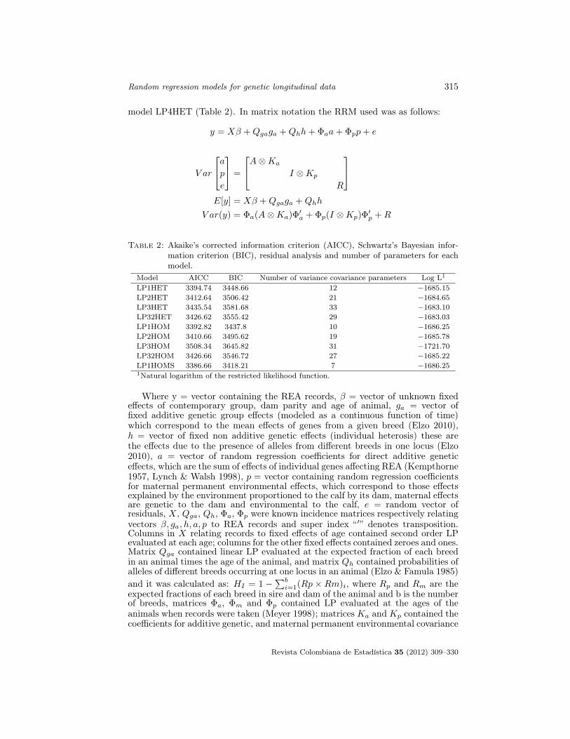
model LP4HET (Table 2). In matrix notation the RRM used was as follows:
y = Xβ +Qgaga +Qhh+ Φaa+ Φpp+ e
V ar
ape
=
A⊗Ka
I ⊗Kp
R
E[y] = Xβ +Qgaga +Qhh
V ar(y) = Φa(A⊗Ka)Φ′a + Φp(I ⊗Kp)Φ′p +R
Table 2: Akaike’s corrected information criterion (AICC), Schwartz’s Bayesian infor-mation criterion (BIC), residual analysis and number of parameters for eachmodel.
Model AICC BIC Number of variance covariance parameters Log L1
LP1HET 3394.74 3448.66 12 −1685.15LP2HET 3412.64 3506.42 21 −1684.65LP3HET 3435.54 3581.68 33 −1683.10LP32HET 3426.62 3555.42 29 −1683.03LP1HOM 3392.82 3437.8 10 −1686.25LP2HOM 3410.66 3495.62 19 −1685.78LP3HOM 3508.34 3645.82 31 −1721.70LP32HOM 3426.66 3546.72 27 −1685.22LP1HOMS 3386.66 3418.21 7 −1686.251Natural logarithm of the restricted likelihood function.
Where y = vector containing the REA records, β = vector of unknown fixedeffects of contemporary group, dam parity and age of animal, ga = vector offixed additive genetic group effects (modeled as a continuous function of time)which correspond to the mean effects of genes from a given breed (Elzo 2010),h = vector of fixed non additive genetic effects (individual heterosis) these arethe effects due to the presence of alleles from different breeds in one locus (Elzo2010), a = vector of random regression coefficients for direct additive geneticeffects, which are the sum of effects of individual genes affecting REA (Kempthorne1957, Lynch & Walsh 1998), p = vector containing random regression coefficientsfor maternal permanent environmental effects, which correspond to those effectsexplained by the environment proportioned to the calf by its dam, maternal effectsare genetic to the dam and environmental to the calf, e = random vector ofresiduals, X, Qga, Qh, Φa, Φp were known incidence matrices respectively relatingvectors β, ga, h, a, p to REA records and super index “ ′” denotes transposition.Columns in X relating records to fixed effects of age contained second order LPevaluated at each age; columns for the other fixed effects contained zeroes and ones.Matrix Qga contained linear LP evaluated at the expected fraction of each breedin an animal times the age of the animal, and matrix Qh contained probabilities ofalleles of different breeds occurring at one locus in an animal (Elzo & Famula 1985)and it was calculated as: HI = 1 −
∑bi=1(Rp × Rm)i, where Rp and Rm are the
expected fractions of each breed in sire and dam of the animal and b is the numberof breeds, matrices Φa, Φm and Φp contained LP evaluated at the ages of theanimals when records were taken (Meyer 1998); matrices Ka and Kp contained thecoefficients for additive genetic, and maternal permanent environmental covariance
Revista Colombiana de Estadística 35 (2012) 309–330
316 Carlos Alberto Martínez, et al.
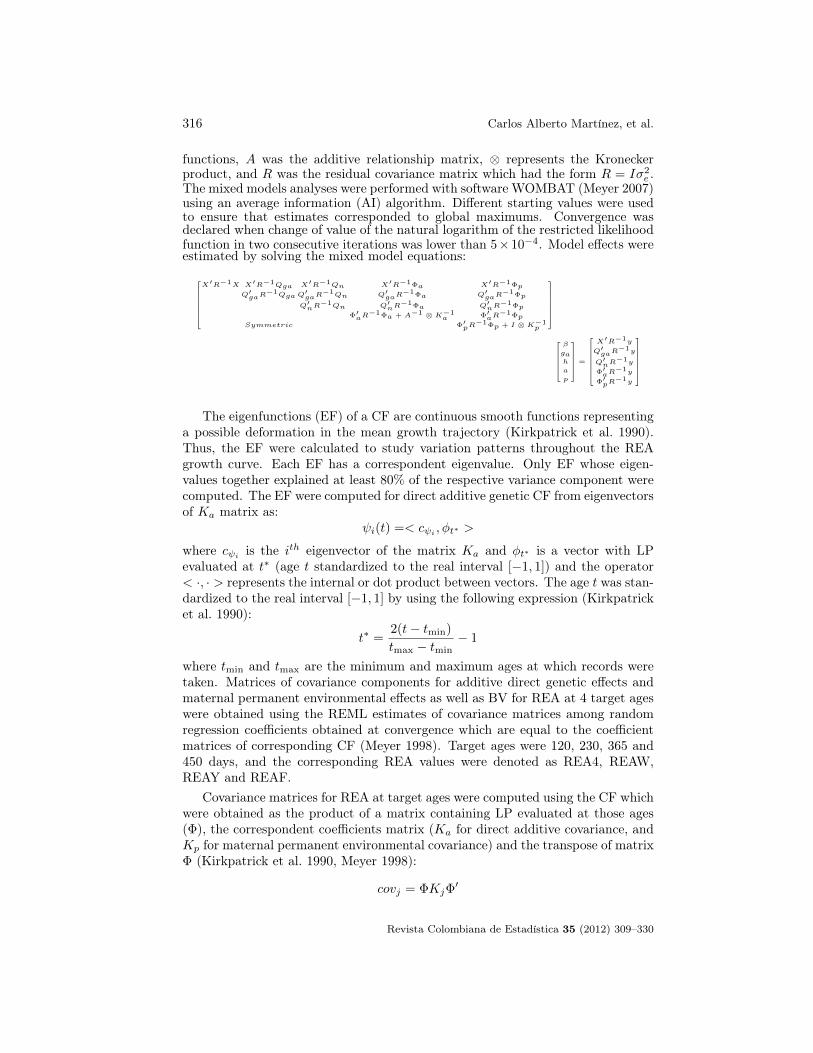
functions, A was the additive relationship matrix, ⊗ represents the Kroneckerproduct, and R was the residual covariance matrix which had the form R = Iσ2
e .The mixed models analyses were performed with software WOMBAT (Meyer 2007)using an average information (AI) algorithm. Different starting values were usedto ensure that estimates corresponded to global maximums. Convergence wasdeclared when change of value of the natural logarithm of the restricted likelihoodfunction in two consecutive iterations was lower than 5×10⁻⁴. Model effects wereestimated by solving the mixed model equations:
X′R−1X X′R−1Qga X′R−1Qn X′R−1Φa X′R−1Φp
Q′gaR−1Qga Q
′gaR−1Qn Q′gaR
−1Φa Q′gaR−1Φp
Q′nR−1Qn Q′nR
−1Φa Q′nR−1Φp
Φ′aR−1Φa + A−1 ⊗K−1
a Φ′aR−1Φp
Symmetric Φ′pR−1Φp + I ⊗K−1
p
β
gah
a
p
=
X′R−1y
Q′gaR−1y
Q′nR−1y
Φ′aR−1y
Φ′pR−1y
The eigenfunctions (EF) of a CF are continuous smooth functions representinga possible deformation in the mean growth trajectory (Kirkpatrick et al. 1990).Thus, the EF were calculated to study variation patterns throughout the REAgrowth curve. Each EF has a correspondent eigenvalue. Only EF whose eigen-values together explained at least 80% of the respective variance component werecomputed. The EF were computed for direct additive genetic CF from eigenvectorsof Ka matrix as:
ψi(t) =< cψi , φt∗ >
where cψi is the ith eigenvector of the matrix Ka and φt∗ is a vector with LPevaluated at t∗ (age t standardized to the real interval [−1, 1]) and the operator< ·, · > represents the internal or dot product between vectors. The age t was stan-dardized to the real interval [−1, 1] by using the following expression (Kirkpatricket al. 1990):
t∗ =2(t− tmin)
tmax − tmin− 1
where tmin and tmax are the minimum and maximum ages at which records weretaken. Matrices of covariance components for additive direct genetic effects andmaternal permanent environmental effects as well as BV for REA at 4 target ageswere obtained using the REML estimates of covariance matrices among randomregression coefficients obtained at convergence which are equal to the coefficientmatrices of corresponding CF (Meyer 1998). Target ages were 120, 230, 365 and450 days, and the corresponding REA values were denoted as REA4, REAW,REAY and REAF.
Covariance matrices for REA at target ages were computed using the CF whichwere obtained as the product of a matrix containing LP evaluated at those ages(Φ), the correspondent coefficients matrix (Ka for direct additive covariance, andKp for maternal permanent environmental covariance) and the transpose of matrixΦ (Kirkpatrick et al. 1990, Meyer 1998):
covj = ΦKjΦ′
Revista Colombiana de Estadística 35 (2012) 309–330
Random regression models for genetic longitudinal data 317
where, Covj is the covariance matrix for the jth covariance component (additivegenetic or maternal permanent environment). The matrix Φ was obtained as theproduct of two matrices. The first is matrix M = (mij)dxk = t∗j−1i , where t∗iis the ith age standardized to the real interval [−1, 1], d is the number of agesconsidered (4 in this case) and k − 1 is the order of the LP. The second matrixwas Λk×k, which contained the coefficients of the LP. Thus, Φ = MΛ (Kirkpatricket al. 1990). Consequently,
Covj = ΦKjΦ′ = MΛKjΛ
′M ′ = MCjM′, where Cj = ΛKjΛ
′
By using matrix Cj instead of matrix Kj for representing the jth CF, covj iscalculated directly as a function of the age standardized to the interval [−1, 1] (i.e.,t∗). This equivalent form was used to compute critical points of CF. The extremesof the CF were also assessed in order to detect the global maximum and minimumvalues of each CF.
The BV were computed for REA4, REAW, REAY and REAF for all individualsin the population (sires, dams, and offspring). The additive breeding value foranimal i at age t (BVit) was computed by adding two terms. The first term was aweighted sum of probabilities of alleles of breed b in animal i times the generalizedleast squares estimate of breed b (deviated from BR) at time t, b = 1, 2, . . . , 7. Thesecond term was the BLUP of the random solution for each individual. This valuewas computed as the internal (or dot) product between a vector containing LPevaluated at age t and a vector whose entries were the BLUP for random regressioncoefficients of animal i. Thus, BVit was computed as:
BVit =< φbt, ga > + < φt, ai >
where φbt is a vector of LP evaluated at the product of the fraction of breed b(b = 1, 2, . . . , 7) in animal i times calf age t standardized to real interval [−1, 1], gais the generalized least squares solution of the fixed coefficient for breed additivegenetic effects, φt is a vector of LP evaluated at calf age t standardized at realinterval [−1, 1], and ai is the BLUP vector of the random coefficients for animal i.
3. Results
3.1. Model Selection
As stated before, estimated covariance functions, covariance components, ge-netic parameters and breeding values were computed using model LP1HOMS.Although this model was selected given the evidence of correlation among mater-nal additive genetic and environmental effects, according to AICC and BIC values,this was the best model since it had the smallest AICC and BIC values (Table 2).
Revista Colombiana de Estadística 35 (2012) 309–330
318 Carlos Alberto Martínez, et al.
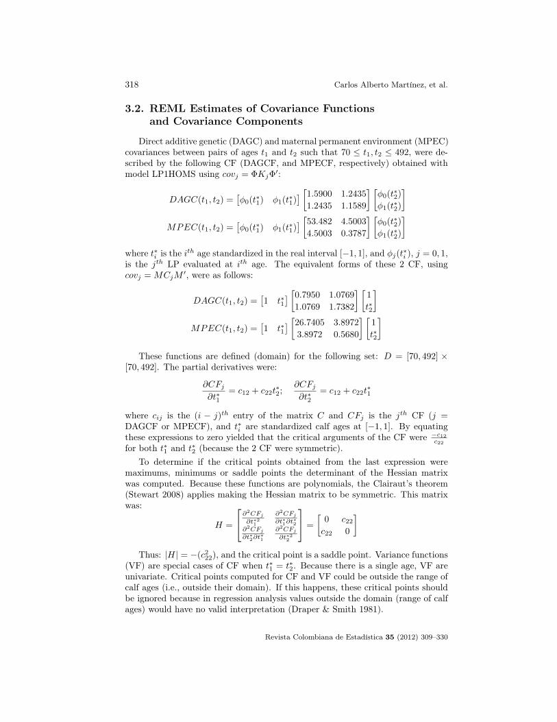
3.2. REML Estimates of Covariance Functionsand Covariance Components
Direct additive genetic (DAGC) and maternal permanent environment (MPEC)covariances between pairs of ages t1 and t2 such that 70 ≤ t1, t2 ≤ 492, were de-scribed by the following CF (DAGCF, and MPECF, respectively) obtained withmodel LP1HOMS using covj = ΦKjΦ
′:
DAGC(t1, t2) =[φ0(t∗1) φ1(t∗1)
] [1.5900 1.2435
1.2435 1.1589
] [φ0(t∗2)
φ1(t∗2)
]MPEC(t1, t2) =
[φ0(t∗1) φ1(t∗1)
] [53.482 4.5003
4.5003 0.3787
] [φ0(t∗2)
φ1(t∗2)
]where t∗i is the ith age standardized in the real interval [−1, 1], and φj(t∗i ), j = 0, 1,is the jth LP evaluated at ith age. The equivalent forms of these 2 CF, usingcovj = MCjM
′, were as follows:
DAGC(t1, t2) =[1 t∗1
] [0.7950 1.0769
1.0769 1.7382
] [1
t∗2
]MPEC(t1, t2) =
[1 t∗1
] [26.7405 3.8972
3.8972 0.5680
] [1
t∗2
]These functions are defined (domain) for the following set: D = [70, 492] ×
[70, 492]. The partial derivatives were:
∂CFj∂t∗1
= c12 + c22t∗2;
∂CFj∂t∗2
= c12 + c22t∗1
where cij is the (i − j)th entry of the matrix C and CFj is the jth CF (j =DAGCF or MPECF), and t∗i are standardized calf ages at [−1, 1]. By equatingthese expressions to zero yielded that the critical arguments of the CF were −c12
c22
for both t∗1 and t∗2 (because the 2 CF were symmetric).To determine if the critical points obtained from the last expression were
maximums, minimums or saddle points the determinant of the Hessian matrixwas computed. Because these functions are polynomials, the Clairaut’s theorem(Stewart 2008) applies making the Hessian matrix to be symmetric. This matrixwas:
H =
∂2CFj∂t∗21
∂2CFj∂t∗1∂t
∗2
∂2CFj∂t∗2∂t
∗1
∂2CFj∂t∗22
=
[0 c22c22 0
]
Thus: |H| = −(c222), and the critical point is a saddle point. Variance functions(VF) are special cases of CF when t∗1 = t∗2. Because there is a single age, VF areunivariate. Critical points computed for CF and VF could be outside the range ofcalf ages (i.e., outside their domain). If this happens, these critical points shouldbe ignored because in regression analysis values outside the domain (range of calfages) would have no valid interpretation (Draper & Smith 1981).
Revista Colombiana de Estadística 35 (2012) 309–330
Random regression models for genetic longitudinal data 319
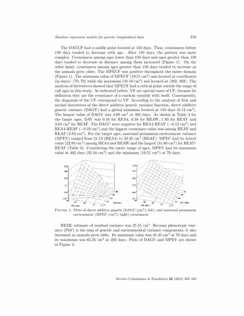
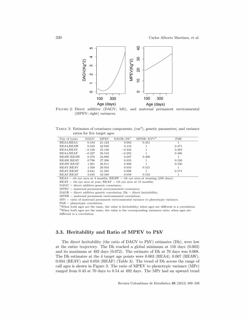
The DAGCF had a saddle point located at 150 days. Thus, covariances before150 days tended to decrease with age. After 150 days, the pattern was morecomplex. Covariances among ages lower than 150 days and ages greater than 150days tended to decrease as distance among them increased (Figure 1). On theother hand, covariances among ages greater than 150 days tended to increase asthe animals grew older. The MPECF was positive throughout the entire domain(Figure 1). The minimum value of MPECF (19.51 cm4) was located at coordinates(in days): (70, 70) while the maximum (35.10 cm4) was located at (492, 492). Theanalysis of derivatives showed that MPECF had a critical point outside the range ofcalf ages in this study. As indicated before, VF are special cases of CF, because bydefinition they are the covariance of a random variable with itself. Consequently,the diagonals of the CF correspond to VF. According to the analysis of first andsecond derivatives of the direct additive genetic variance function, direct additivegenetic variance (DAGV) had a global minimum located at 150 days (0.13 cm4).The largest value of DAGV was 4.69 cm4 at 492 days. As shown in Table 3 forthe target ages, DAV was 0.16 for REA4, 0.38 for REAW, 1.93 for REAY and3.64 cm4 for REAF. The DAGC were negative for REA4-REAY (−0.13 cm4) andREA4-REAF (−0.23 cm4) and the biggest covariance value was among REAY andREAF (2.64 cm4). For the target ages, maternal permanent environment variance(MPEV) ranged from 21.12 (REA4) to 33.35 cm4 (REAF). MPEC had its lowestvalue (22.93 cm4) among REA4 and REAW and the largest (31.60 cm4) for REAY-REAF (Table 3). Considering the entire range of ages, MPEV had its maximumvalue at 492 days (35.10 cm4) and the minimum (19.51 cm4) at 70 days.
Figure 1: Plots of direct additive genetic (DAGC (cm4); left), and maternal permanentenvironment (MPEC (cm4); right) covariances.
REML estimate of residual variance was 25.55 cm4. Because phenotypic vari-ance (PhV) is the sum of genetic and environmental variance components, it alsoincreased as animals grew older. Its minimum value was 45.45 cm4 at 70 days andits maximum was 65.35 cm4 at 492 days. Plots of DAGV and MPEV are shownin Figure 2.
Revista Colombiana de Estadística 35 (2012) 309–330
320 Carlos Alberto Martínez, et al.
100 300
01
23
45
Age (days)
DAG
V(K
g^2)
100 300
010
2030
40
Age(days)
MP
EV
(Kg^
2)
100 300
01
23
45
Age(days)
DAG
V(K
g^2)
100 300
010
2030
40
Age (days)
MP
EV
(Kg^
2)
Figure 2: Direct additive (DAGV; left), and maternal permanent environmental(MPEV; right) variances.
Table 3: Estimates of covariance components, (cm4), genetic parameters, and varianceratios for five target ages.
Pair of traits DAGC MPEC DAGR/Dh1 MPER/MPr2 PhRREA4,REA4 0.164 21.124 0.003 0.451 1REA4,REAW 0.033 22.930 0.133 1 0.471REA4,REAY −0.126 25.146 −0.224 1 0.483REA4,REAF −0.227 26.542 −0.294 1 0.486REAW,REAW 0.376 24.890 0.007 0.490 1REAW,REAY 0.796 27.296 0.935 1 0.520REAW,REAF 1.061 28.811 0.908 1 0.530REAY,REAY 1.928 29.934 0.034 0.521 1REAY,REAF 2.641 31.595 0.998 1 0.571REAF,REAF 3.635 33.349 0.058 0.533 1REA4 = rib eye area at 4 months; REAW = rib eye area at weaning (230 days);REAY = rib eye area at year; REAF = rib eye area at 15 months;DAGC = direct additive genetic covariance;MPEC = maternal permanent environmental covariance;DAGR = direct additive genetic correlation; Dh = direct heritability;MPER = maternal permanent environmental correlation;MPr = ratio of maternal permanent environmental variance to phenotypic variance;PhR = phenotypic correlation.1When both ages are the same, the value is heritability; when ages are different is a correlation.2When both ages are the same, the value is the corresponding variances ratio; when ages aredifferent is a correlation.
3.3. Heritability and Ratio of MPEV to PhV
The direct heritability (the ratio of DAGV to PhV) estimates (Dh), were lowat the entire trajectory. The Dh reached a global minimum at 150 days (0.003)and its maximum at 492 days (0.072). The estimate of Dh at 70 days was 0.008.The Dh estimates at the 4 target age points were 0.003 (REA4), 0.007 (REAW),0.034 (REAY) and 0.058 (REAF) (Table 3). The trend of Dh across the range ofcalf ages is shown in Figure 3. The ratio of MPEV to phenotypic variance (MPr)ranged from 0.43 at 70 days to 0.54 at 492 days. The MPr had an upward trend
Revista Colombiana de Estadística 35 (2012) 309–330
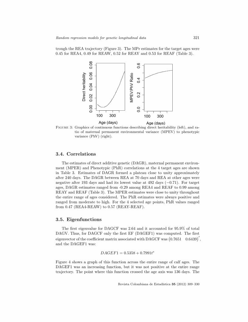
Random regression models for genetic longitudinal data 321
trough the REA trajectory (Figure 3). The MPr estimates for the target ages were0.45 for REA4, 0.49 for REAW, 0.52 for REAY and 0.53 for REAF (Table 3).
100 300
0.00
0.02
0.04
0.06
0.08
Age (days)
Dire
ct h
erita
bilit
y
100 300
0.0
0.2
0.4
0.6
Age(days)
MP
EV:
PhV
Rat
io
100 300
0.00
0.02
0.04
0.06
0.08
Age(days)
Dire
ct h
erita
bilit
y
100 300
0.0
0.2
0.4
0.6
Age (days)
MP
EV:
PhV
Rat
ioFigure 3: Graphics of continuous functions describing direct heritability (left), and ra-
tio of maternal permanent environmental variance (MPEV) to phenotypicvariance (PhV) (right).
3.4. Correlations
The estimates of direct additive genetic (DAGR), maternal permanent environ-ment (MPER) and Phenotypic (PhR) correlations at the 4 target ages are shownin Table 3. Estimates of DAGR formed a plateau close to unity approximatelyafter 240 days. The DAGR between REA at 70 days and REA at other ages werenegative after 193 days and had its lowest value at 492 days (−0.71). For targetages, DAGR estimates ranged from -0.29 among REA4 and REAF to 0.99 amongREAY and REAF (Table 3). The MPER estimates were close to unity throughoutthe entire range of ages considered. The PhR estimates were always positive andranged from moderate to high. For the 4 selected age points, PhR values rangedfrom 0.47 (REA4-REAW) to 0.57 (REAY-REAF).
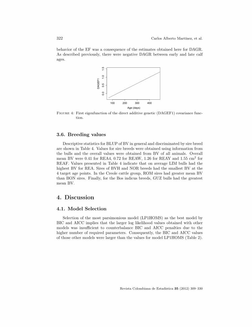
3.5. Eigenfunctions
The first eigenvalue for DAGCF was 2.64 and it accounted for 95.9% of totalDAGV. Thus, for DAGCF only the first EF (DAGEF1) was computed. The firsteigenvector of the coefficient matrix associated with DAGCF was
(0.7651 0.6439
)′,
and the DAGEF1 was:
DAGEF1 = 0.5358 + 0.7991t∗
Figure 4 shows a graph of this function across the entire range of calf ages. TheDAGEF1 was an increasing function, but it was not positive at the entire rangetrajectory. The point where this function crossed the age axis was 136 days. The
Revista Colombiana de Estadística 35 (2012) 309–330
322 Carlos Alberto Martínez, et al.
behavior of the EF was a consequence of the estimates obtained here for DAGR.As described previously, there were negative DAGR between early and late calfages.
100 200 300 4000.
00.
51.
01.
5
Age (days)
DA
GE
F1
Figure 4: First eigenfunction of the direct additive genetic (DAGEF1) covariance func-tion.
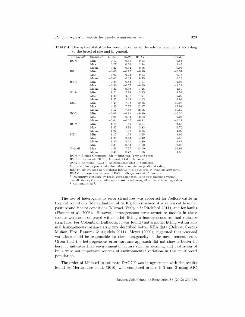
3.6. Breeding values
Descriptive statistics for BLUP of BV in general and discriminated by sire breedare shown in Table 4. Values for sire breeds were obtained using information fromthe bulls and the overall values were obtained from BV of all animals. Overallmean BV were 0.41 for REA4, 0.72 for REAW, 1.26 for REAY and 1.55 cm2 forREAF. Values presented in Table 4 indicate that on average LIM bulls had thehighest BV for REA. Sires of BVH and NOR breeds had the smallest BV at the4 target age points. In the Creole cattle group, ROM sires had greater mean BVthan BON sires. Finally, for the Bos indicus breeds, GUZ bulls had the greatestmean BV.
4. Discussion
4.1. Model Selection
Selection of the most parsimonious model (LP1HOMS) as the best model byBIC and AICC implies that the larger log likelihood values obtained with othermodels was insufficient to counterbalance BIC and AICC penalties due to thehigher number of required parameters. Consequently, the BIC and AICC valuesof those other models were larger than the values for model LP1HOMS (Table 2).
Revista Colombiana de Estadística 35 (2012) 309–330
Random regression models for genetic longitudinal data 323
Table 4: Descriptive statistics for breeding values at the selected age points accordingto the breed of sire and in general.
Sire breed1 Statistic2 REA4 REAW REAY REAFBON Min 0.17 0.35 0.53 0.63
Max 0.27 0.56 1.14 1.47Mean 0.22 0.42 0.76 0.95
BR Min −0.07 −0.17 −0.40 −0.54Max 0.02 0.22 0.53 0.73Mean −0.02 0.05 0.13 0.19
BVH Min −0.34 −0.83 −1.61 −2.06Max −0.30 −0.57 −0.99 −1.21Mean −0.32 −0.69 −1.26 −1.59
GUZ Min 1.22 2.18 3.73 4.58Max 1.29 2.37 4.24 5.29Mean 1.25 2.29 4.03 4.99
LIM Min 4.49 7.32 12.36 15.06Max 4.56 7.57 12.97 15.91Mean 4.52 7.48 12.76 15.62
NOR Min −0.09 −0.11 −0.20 −0.30Max 0.06 −0.03 0.03 0.07Mean −0.04 −0.07 −0.11 −0.14
ROM Min 1.15 1.86 3.04 3.65Max 1.25 2.16 3.83 4.76Mean 1.22 1.98 3.35 4.09
SIM Min 1.17 1.95 3.25 3.95Max 1.25 2.43 4.42 5.55Mean 1.20 2.21 3.89 4.83Min −0.34 −0.83 −1.60 −2.06
Overall Max 4.56 7.57 13.00 15.91Mean 0.41 0.72 1.26 1.55
BON = Blanco Orejinegro; BR = Brahman (gray and red);BVH = Braunvieh; GUZ = Guzerat; LIM = Limousin;NOR = Normand; ROM = Romosinuano; SIM = Simmental;Min = minimum predicted value; Max = maximum predicted value;REA4= rib eye area at 4 months; REAW = rib eye area at weaning (230 days);REAY= rib eye area at year; REAF = rib eye area at 15 months.1 Descriptive statistics by breed were computed using sires breeding values;overall: descriptive statistics were constructed using all animals’ breeding values2 All units in cm2.
The use of heterogeneous error structures was reported for Nellore cattle intropical conditions (Mercadante et al. 2010), for crossbred Australian cattle underpasture and feedlot conditions (Mirzaei, Verbyla & Pitchford 2011), and for lambs(Fischer et al. 2006). However, heterogeneous error structure models in thesestudies were not compared with models fitting a homogeneous residual variancestructure. For Colombian Buffaloes, it was found that a model fitting within ani-mal homogeneous variance structure described better REA data (Bolívar, Cerón-Muñoz, Elzo, Ramírez & Agudelo 2011). Meyer (2000), suggested that seasonalvariations could be responsible for the heterogeneity in the measurement error.Given that the heterogeneous error variance approach did not show a better fithere, it indicates that environmental factors such as weaning and castration ofbulls were not important sources of environmental variation in this multibreedpopulation.
The order of LP used to estimate DAGCF was in agreement with the resultsfound by Mercadante et al. (2010) who compared orders 1, 2 and 3 using AIC
Revista Colombiana de Estadística 35 (2012) 309–330
324 Carlos Alberto Martínez, et al.
and BIC as model selection criteria. However, they did not consider LP of order1 to model random non genetic effects. In that study, orders of LP to modelthose effects were either 2 or 3. Mercadante et al. (2010) found that the modelconsidering the lower orders of fit for both direct additive genetic and permanentenvironmental effects was the best 1. The LP of order one were also reported tobe sufficient to explain direct additive genetic effects for weight data in crossbredcattle cows (Arango, Cundiff & Van Vleck 2004).
Considering the small size of the dataset in this study and that a model withonly 7 parameters that permitted the use of all records was selected, RRM seemto be a good option to model longitudinal ultrasound data. If a four-trait modelassuming zero covariance between direct and maternal additive effects had beenfitted here, the number of parameters needed would have been 4×(4×(4+1)/2) =40, which is more than 4 times greater than the number of parameters estimatedwith the LP1HOMS model. Even if two-trait models had been utilized, a total of 6two-trait analysis would have had to be performed to estimate the full covariancematrix for REA at the 4 target ages. In addition, because each analysis wouldbe performed separately, there would have been no certainty for the estimatedsix-trait covariance matrix to be positive definite.
4.2. REML Estimates of Covariance Functions andCovariance Components
The direct additive genetic variance function corresponding to the DAGCFwhen t1 = t2 (Figure 2) was concave up with a global minimum at 150 days of age.Thus, the increase in the magnitude of the variance after the minimum point wasalways positive and greater as the animals grew older. Among the few literaturereports using RRM to model ultrasound longitudinal data, a smoother pattern forDAGV (in the age interval 60 to 360 days) was reported for eye muscle depth (aultrasonic measure at the same point where REA is taken, but measuring depthnot area) in lambs (Fischer et al. 2006). Although they found that additive geneticvariance did not have great changes, it had a concave up shape. A Nellore cattlestudy under pasture and feedlot conditions in a tropical region was conducted byMercadante et al. (2010) in Brazil. However they did not discuss the covariancetendencies. The very low values of DAGV around 150 days here may have beendue to computing artifacts rather than biology. Numerical problems have beenreported for RRM using LP as base functions (Nobre, Misztal, Tsuruta, Bertrand,Silva & Lopes 2003, Bohmanova, Misztal & Bertrand 2005, Bertrand, Misztal,Robins, Bohmanova & Tsuruta 2006).
The DAGV did not decrease after weaning but it increased with the calf’s age.Maternal effects have been found to be important for REA and other ultrasoundtraits (Speidel et al. 2007). These results suggested that maternal effects wouldneed to be considered in models for genetic analysis of postweaning growth traits.No other literature reports were found for longitudinal REA data considering ma-ternal effects in cattle.
Revista Colombiana de Estadística 35 (2012) 309–330
Random regression models for genetic longitudinal data 325
4.3. Heritability and Ratio of MPEV to PhV
The Dh values followed the same trajectory as DAGV. Low values of Dh (partic-ularly at 150 days) could be due to numerical problems related to the populationstructure and small size of dataset. The only literature report found for Dh ofREA in cattle using RRM showed higher values than those reported in the currentstudy. That study considered a range of ages from 323 to 773 days in a BrazilianNellore cattle population and Dh estimates ranged from 0.31 to 0.42 (Mercadanteet al. 2010). The Dh for REA at slaughter for Australian crossbred cattle in pas-ture conditions until 18 months of age and then placed in feedlot conditions wasestimated to be 0.40 (Mirzaei et al. 2011). In a Colombian purebred Brahmanpopulation under similar management conditions (pastures and mineral supple-mentation) to those in this study, Dh for REAF was 0.37 (Jiménez et al. 2010).For Red Angus animals of ages between 300 and 480 days and with a single ultra-sonic REA measurement, Speidel et al. (2007) found a Dh estimate of 0.35. Crews& Kemp (1999) suggested that maternal effects were unimportant for the geneticevaluation of carcass traits (including REA) in a multibreed population. However,they did not use RRM because they considered REA data only at slaughter. Thus,differences in the data structure (longitudinal vs. simple), the model used, andthe fact that presumably maternal effects have a small effect on traits measuredat slaughter could explain the different results. In agreement with results here, forRed Angus cattle, Speidel et al. (2007) concluded (based on a likelihood ratio test)that inclusion of maternal effects improved the ability of genetic models to accountfor variability on carcass traits. The MPr estimates increased smoothly with age.The MPr had medium to high values across all ages and had a total (maximumvalue - minimum value) change of 10.8 percentage units. For live weight, undersimilar conditions and for a Bos indicus (Nellore) beef cattle population, Albu-querque & Meyer (2001) found a similar pattern for MPr. No research includingmaternal permanent environmental effects for REA data in cattle was found inthe literature. The MPr values did not decrease after weaning, thus, the perma-nent maternal environmental effects were important for post weaning developmentphases. This suggests that remnants of pre-weaning permanent environmental coweffects continued to influence calf REA until 492 days of age. Maternal effects aremainly explained for cow’s milk production (genetic to the dam and environmentalto the calf). Considering the values of MPr (0.43 to 0.54), it seems that a keypoint to obtain animals with greater REA, which are expected to have a greatermeat production, would be to implement an adequate selection program that in-cludes both direct growth and maternal milk production. It has to be taken intoaccount that although maternal additive genetic effects were not included in themodel due to estimation problems, they are still present. On the other hand, theunique maternal effect term in the model is possibly accounting for both: Additivegenetic and permanent environment maternal effects.
Revista Colombiana de Estadística 35 (2012) 309–330
326 Carlos Alberto Martínez, et al.
4.4. Correlations
As the DAGR formed a plateau after approximately 240 days, for genetic eval-uation purposes, when considering REA data with ages greater than 240 days (forexample, from weaning to greater ages), it will be possible to use a repeatabilitymodel. The simplicity of this model will make it desirable, especially for smalldata sets as present one. For live weight records, a similar conclusion was foundby Arango et al. (2004) for crossbred beef cows in a temperate region.
The negative DAGR between ages at the beginning of the trajectory and finalages indicated that those genes controlling REA at ages near to 70 days are antag-onist to genes controlling this trait at ages near to 492 days. Taking into accountthat what matters is REA at ages near slaughter, animals could be selected forREA at ages after 240 days (because of the plateau formed by DAGR occurredafter that point). Because MPER values were medium to high across calf ages, itappears that maternal permanent environmental effects exerted a positive effecton REA preweaning, and this effect persisted until 492 days of age. As a gen-eral observation taking into account, MPr and MPER values for this population,maternal effects appeared to be important to obtain greater REA.
4.5. Eigenfunctions
The proportion of DAGV explained by the first eigenvalue (95.9%) was in therange of proportions found by Mercadante et al. (2010). Such range was 84% to99% depending on the model used. A similar proportion (90%) was describedfor Longissimus muscle depth at the same point where REA was taken in lambs(Fischer et al. 2006). As the DAGEF1 crossed the age axis at 136 days, thisis a critical age because selection for greater REA values before this trajectorypoint will tend to negatively deform the mean population REA growth curve forlater ages. Considering only ages after that point, selection for direct additivegenetic effects will increase REA mean population growth curve. Thus, selectionfor REA could be performed after 136 days, i.e., roughly 4 months of age underfield conditions. However, considering the high DAGR between 136 days and 240days of age, a practical age to perform selection for REA would be at weaning.
4.6. Breeding Values
Given the small number of sires considered in the current study (especially forBos taurus breeds) results should be viewed with caution. As expected, all geneticadditive direct breed effects were estimable. Thus, the use of orthogonal functionsto describe fixed genetic effects when modeling longitudinal data could be useful inorder to prevent estimability problems. No research that considered breed effectsas a continuous function of age of calf was found in the literature.
Range of BV for REAF of BR sires (Table 4) was smaller than the rangereported by Jiménez et al. (2010) for purebred Brahman cattle under pasture con-ditions in Colombia. They reported EPD values ranging from −2.84 to 3.47 cm2,
Revista Colombiana de Estadística 35 (2012) 309–330
Random regression models for genetic longitudinal data 327
thus, the BV (twice the EPD) ranged from −5.68 to 6.94 cm2. As in the currentstudy, BV were deviated from BR. The range of BV for purebred BR animals(non parents; −0.82 to 1.12 cm2) was smaller than those reported by Jiménezet al. (2010) suggesting that the amount of genetic variability in the dataset herewas smaller than in the Brahman population analyzed by these authors.
The BLUP of BV suggested that among the tested sires and under the con-ditions of the study LIM bulls had the greatest mean genetic merit for REA atall target ages (Table 4). When all of the sires were ranked according to individ-ual BV, LIM sires were always those with the greatest values. Consequently, theLIM breed would have to be considered for crossbreeding programs with Brahmancows under pasture conditions in the Southern Cesar region of Colombia. TheLIM breed had been reported to have greater additive genetic effects for REA atdifferent ages when compared to Bos indicus and Bos taurus breeds in temperateareas under feedlot or high supplement conditions (Ríos-Utrera, Cundiff, Gregory,Koch, Dikeman, Koohmaraie & Van Vleck 2006, Williams, Aguilar, Rekaya &Bertrand 2010). According to the results of this research, in tropical regions andunder pasture conditions, LIM animals also showed a good performance for thistrait.
5. Final Remarks
It should be mentioned that genetic parameters and breeding values were es-timated with limited accuracy due to the structure and small size of the availablemultibreed population. Estimates of (co)variance components showed that it isnecessary to validate the results of this research with substantially larger multi-generational populations before implement RRM in regional or national geneticevaluation procedures. Thus, there is a need to continue obtaining longitudinalultrasound information from different beef cattle herds where the breeds studiedhere are represented. Results suggested that maternal effects were important, bothpreweaning and postweaning. Thus, maternal effects (genetic and non-genetic) ap-peared to be relevant effects to be included in models for genetic evaluation of REApre and postweaning under pasture conditions in Colombia.
Acknowledgments
We sincerely thank two referees for helpful comments and suggestions whichled to improve this paper.
[Recibido: agosto de 2011 — Aceptado: abril de 2012
]Revista Colombiana de Estadística 35 (2012) 309–330
328 Carlos Alberto Martínez, et al.
References
Albuquerque, L. G. & Meyer, K. (2001), ‘Estimates of covariance functions forgrowth from birth to 630 days of age in nellore cattle’, Journal of AnimalScience 79(1), 2776–2789.
Arango, J. A., Cundiff, L. V. & Van Vleck, L. (2004), ‘Covariance functions andrandom regression models for cow weight in beef cattle’, Journal of AnimalScience 82(1), 54–67.
Bertrand, J. K., Misztal, I., Robins, K. R., Bohmanova, J. & Tsuruta, S. (2006),Implementation of random regression models for large scale evaluations forgrowth in beef cattle, in ‘Proceedings of the 8th World Congress on GeneticApplied to Livestock Production’, Minas Gerais: Sociedade Brasileira de Mel-horamiento Animal, Belo Horizonte.
Bohmanova, J., Misztal, I. & Bertrand, J. K. (2005), ‘Studies on multiple traitand random regression models for genetic evaluation of beef cattle for growth’,Journal of Animal Science 83(1), 62–67.
Bolívar, D. M., Cerón-Muñoz, M. F., Elzo, M. A., Ramírez, E. J. & Agudelo, D. A.(2011), ‘Growth curves for buffaloes (Bubalus bubalis) using random regres-sion mixed models with different structures of residual variances’, Journal ofAnimal Science 89(1), 62–67. Suppl E1: 530.
Choy, Y. H., Lee, C. W., Kim, H. C., Choi, S. B., Choi, J. G. & Hwang, J. M.(2008), ‘Genetic models for carcass traits with different slaughter endpoints inselected hanwoo herds I. linear covariance models’, Journal of Animal Science21, 1227–1232.
Crews, D. H. & Kemp, R. A. (1999), ‘Contributions of preweaning growth infor-mation and maternal effects for prediction of carcass trait breeding valuesamong crossbred beef cattle’, Journal of Animal Science 79, 17–25.
Draper, N. R. & Smith, H. (1981), Applied regression analysis, 2 edn, John Wiley& Sons Inc., New York.
Elzo, M. A. (2010), Animal breeding notes, University of Florida, Gainesville.
Elzo, M. A. & Famula, T. R. (1985), ‘Multibreed sire evaluation procedures withina country’, Journal of Animal Science 60, 942–952.
Elzo, M. A. & Wakeman, D. L. (1998), ‘Covariance components and predictionfor additive and nonadditive preweaning growth genetic effects in an angus-brahman multibreed herd’, Journal of Animal Science 76, 1290–1302.
FEDEGAN (2006), Plan estratégico de la ganadería colombiana 2019, San MartinObregon y Cía, Bogotá, D.C.
Fischer, T. M., van der Werf, J. H. J., Banks, R. G., Ball, A. J. & Gilmour, A. R.(2006), ‘Genetic analysis of weight, fat and muscle depth in growing lambsusing random regression models’, Journal of Animal Science 82, 13–22.
Revista Colombiana de Estadística 35 (2012) 309–330
Random regression models for genetic longitudinal data 329
Hassen, A., Wilson, D. E. & Rouse, G. H. (2003), ‘Estimation of genetic parametersfor ultrasound-predicted percentage of intramuscular fat in angus cattle usingrandom regression models’, Journal of Animal Science 81, 35–45.
Hougton, P. L. & Turlington, L. M. (1992), ‘Application of ultrasound for feedingand finishing animals: A review’, Journal of Animal Science 70, 930–941.
Jiménez, A., Manrique, C. & Martínez, C. A. (2010), ‘Parámetros y valores genéti-cos para características de composición corporal, área de ojo del lomo y grasadorsal medidos mediante ultrasonido en la raza brahman’, Revista MedicinaVeterinaria y Zootecnica 57, 178–190.
Kempthorne, O. (1957), An Introduction to Genetic Statistics, John Wiley.
Kirkpatrick, M., Lofsvold, D. & Bulmer, M. (1990), ‘Analysis of the inheritance,selection and evolution of growth trajectories’, Genetics 124, 979–993.
Littell, R. C., Milliken, G. A., Stroup, W. W., Wolfinger, R. D. & Schabenberger,O. (2006), SAS for Mixed Models, Cary (NC): SAS Institute Inc.
Lynch, M. & Walsh, B. (1998), Genetic and Analysis of Quantitative Traits, Sin-auer Associates, Inc., Arizona.
Mercadante, M. E. Z., El Faro, L., Pinheiro, T. R., Cyrillo, J. N. S. G., Bonilha,S. F. M. & Branco, R. H. (2010), Estimation of heritabality and repeatabilityfor ultrasound carcass traits in nelore cattle using random regression models,in ‘Proceedings of the 9th World Congress on Genetic Applied to LivestockProduction’, Leipzig.
Meyer, K. (1998), ‘Estimating covariance functions for longitudinal data using arandom regression model’, Genetics Selection Evolution 38, 221–240.
Meyer, K. (2000), ‘Random regression to model phenotypic variation in monthlyweights of australian beef cattle’, Livestock Production Science 65, 19–38.
Meyer, K. (2007), ‘WOMBAT -A program for mixed models analyses in quantita-tive genetics by REML’, Journal of Zhejiang University Science B 8, 815–821.
Meyer, K. & Hill, W. G. (1997), ‘Estimation of genetic and phenotypic covari-ance functions for longitudinal or “repeated” records by restricted maximumlikelihood’, Livestock Production Science 47, 185–200.
Mirzaei, H. R., Verbyla, A. P. & Pitchford, W. S. (2011), ‘Joint analysis of beefgrowth and carcass quality traits through calculation of co-variance compo-nents and correlations’, Genetics and Molecular Research 10, 433–447.
Nobre, P. R. C., Misztal, I., Tsuruta, S., Bertrand, J. K., Silva, L. O. C. & Lopes,P. S. (2003), ‘Analysis of growth curves of nellore cattle by multiple-trait andrandom regression models’, Journal of Animal Science 81, 918–926.
Revista Colombiana de Estadística 35 (2012) 309–330
330 Carlos Alberto Martínez, et al.
Ríos-Utrera, A., Cundiff, L. V., Gregory, K. E., Koch, R. M., Dikeman, M. E.,Koohmaraie, M. & Van Vleck, L. D. (2006), ‘Effects of age, weight, and factslaughter end points on estimates of breed and retained heterosis effects forcarcass traits’, Journal of Animal Science 84, 63–87.
Speidel, S. E., Enns, R. M., Brigham, B. W. & Keeman, L. D. (2007), ‘Geneticparameter estimates for ultrasound indicators of carcass’, Journal of AnimalScience 58, 39–42.
Stewart, J. (2008), Cálculo en varias variables. Trascendentes tempranas, 6 edn,Cengage Learning, México DF.
Van Soest, P. J. (1994), Nutritional Ecology of the Ruminant, 2 edn, ComstockPublishing Sssociates, New York.
Williams, J. L., Aguilar, I., Rekaya, R. & Bertrand, J. K. (2010), ‘Estimationof breed and heterosis effects for growth and carcass traits in cattle usingpublished crossbreeding studies’, Journal of Animal Science 88, 460–466.
Wilson, D. E. (1992), ‘Application of ultrasound for genetic improvement’, Journalof Animal Science 70, 973–983.
Revista Colombiana de Estadística 35 (2012) 309–330