random walks on random graphs - university of british ...barlow/talks/iciam.pdf · random walks on...

Random walks on random graphs

Martin Barlow

Department of Mathematics

University of British Columbia

Random walks on random graphs – p. 1/24

Random walks in random environment on Zd

There are two common models for random walk in a random environment inZd:

‘Random walk in random environment’ (RWRE). i.i.d. random transitionprobabilities out of each pointx ∈ Z

d. This model is hard, because in general it isnot symmetric (i.e. reversible). There are still many open problems. I will not talkabout this model.

‘Random conductance model’ (RCM). As we’ll see, now quite well understood.

Intuitive description: put i.i.d. random conductances (orweights)ωe ∈ [0,∞) onthe edges of the Euclidean lattice(Zd, Ed). Look at a continuous time MarkovchainXt with jump probabilities proportional to the edge conductances.

So if X0 = x then the jump probability fromx to y ∼ x is

Pxy =ωxy∑

z∼x ωxz.


Example

Bond conductivities:blue ≪ 1, black≈ 1, red ≫ 1.


Definitions

Environment. Fix a probability measureκ on [0,∞). Let Ω = [0,∞]Ed be thespace of environments, and letP be the probability law onΩ which makes thecoordinatesωe, e ∈ Ed i.i.d. with law κ.Choose a ‘speed measure’νx(ω), x ∈ Z

d. (How? See next slide....)

Random walk. Let Ω′ = D([0,∞), Zd) be the space of (right cts left limit) paths.For eachω ∈ Ω let P x

ω be the probability law onΩ′ which makes the coordinateprocessXt = Xt(ω

′) a Markov chain with generator

Lνf(x) =1

νx

∑y∼x

ωxy(f(y) − f(x)).

Write ωxy = 0 if x 6∼ y, andµx =∑

y ωxy.Thenν is a stationary measure forX , X is reversible (symmetric) with respect toν, and the overall jump rate out ofx is µx/νx.


Choice of the ‘speed measure’ ν

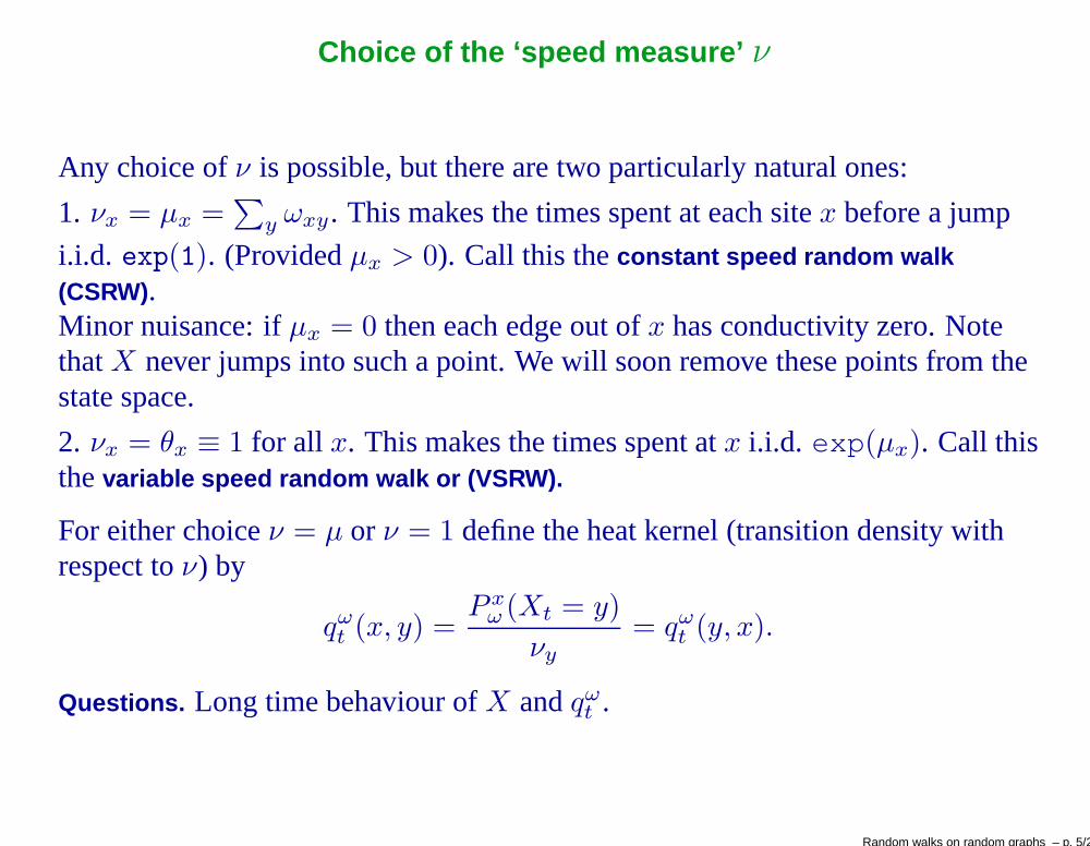
Any choice ofν is possible, but there are two particularly natural ones:

1. νx = µx =∑

y ωxy. This makes the times spent at each sitex before a jump

i.i.d. exp(1). (Providedµx > 0). Call this theconstant speed random walk(CSRW).Minor nuisance: ifµx = 0 then each edge out ofx has conductivity zero. NotethatX never jumps into such a point. We will soon remove these points from thestate space.

2. νx = θx ≡ 1 for all x. This makes the times spent atx i.i.d. exp(µx). Call thisthevariable speed random walk or (VSRW).

For either choiceν = µ or ν = 1 define the heat kernel (transition density withrespect toν) by

qωt (x, y) =

P xω (Xt = y)

νy= qω

t (y, x).

Questions. Long time behaviour ofX andqωt .


Percolation and positive conductance bonds

If ωe = 0 thenX cannot jump across the edgee. Define a percolation processassociated with the environmentω by taking

x, y is open ⇔ ωxy > 0,

and letCx = Cx(ω) be the open cluster containingx – i.e. the set ofy ∈ Zd such

thatx andy are connected by a path of open edges. So

P xω (Xt ∈ Cx for all t ≥ 0) = 1.

Letp+ = P(ωe > 0).

If p+ < pc(d), the critical probability for bond percolation inZd, then all theopen clusters are finite, soX is trapped in a small finite region.


Bond percolation with p+ = 0.2.


GB and QFCLT

Assumption. From now on assume

p+ > pc(d).

Write C∞(ω) for the (P-a.s. unique) infinite cluster of the associated percolationprocess, and considerX started only at points inC∞(ω).

Problems. What we would like to have (but may not):

Gaussian bounds (GB)on qωt (x, y).

Quenched functional CLT with diffusivityσ2: Let X(n)t = n−1/2Xnt, andW be a

BM(Rd). Then forP-a.a.ω, underP 0ω,

X(n) ⇒ σW.

(In particular isσ2 > 0?)


Gaussian bounds in the random context

For GB one wants:

For eachx ∈ Zd there exist r.v.Tx(ω) ≥ 1 with

P(Tx ≥ n, x ∈ C∞) ≤ c exp(−nεd) (T )

and (non-random) constantsci = ci(d, p) such that the transition density ofXsatisfies,

c1

td/2e−c2|x−y|2/t ≤ qω

t (x, y) ≤c3

td/2e−c4|x−y|2/t, (GB)

for x, y ∈ C∞(ω), t ≥ max(Tx(ω), c|x − y|).

1. The randomness of the environment is taken care of by theTx(ω), which willbe small for most points, and large for the rare points in large ‘bad regions’.2. Good control of the tails of the r.v.Tx, as in (T), is essential for applications.


Consequences of GB and QFCLT

GB lead to Harnack inequalities, which imply Hölder continuity of harmonicfunctions, solutions of the heat equation onC∞, and Green’s functions.

However: define theslabSN = x = (x1, . . . , xd) ∈ Zd : |x1| < N. We would

guess that

limN→∞

P 0ω(X leavesSN upwards, i.e. inx : x1 > 0 ) = 1

2 , (∗)

but (GB) do not imply this.

QFCLT does imply (*), but on its own does not give good controlof harmonicfunctions.

If one has both GB and QFCLT then one obtains a local limit theorem forqωt (x, y) (MB + B. Hambly) and good control of Green’s functions.


Averaged FCLT

Recall that

X(n)t = n−1/2Xnt.

For eventsF ⊂ Ω × Ω′ define

E∗(1F ) = EE0

ω1F , and writeP∗ for the associated probability.

Theorem A. (De Masi, Ferrari, Goldstein, Wick 1989). Let(ωe, e ∈ Ed) be ageneral stationary ergodic environment. Assume thatEωe < ∞. UnderP∗,X(n) ⇒ σW, whereW is a BM, andσ2 ≥ 0.

This gives a FCLT, but one where we average over all environments.

This paper used the Kipnis-Varadhan approach of ‘the environment seen from theparticle’.

We have no example of a environment satisfying the conditions of Theorem A forwhich the QFLCT fails. But work in progress (MB-Burdzy-Timar) shows thatmore generally it is possible to have AFCLT without QFCLT.


Special cases for the law of ωe.

1. “Elliptic” : 0 < C1 ≤ ωe ≤ C2 < ∞.2. “Percolation”: ωe ∈ 0, 1 (andp+ > pc.)3. “Bounded above”: ωe ∈ [0, 1] (andp+ > pc.)4. “Bounded below”: ωe ∈ [1,∞).

In Cases 1–3 there is little difference between the CSRW and the VSRW.

1. Elliptic case.GB follow from general results of Delmotte (1999).QFCLT was only proved in full generality by Sidoravicius andSznitman (2004).

2. Percolation. GB proved by MB (2004). QFCLT proved by Sidoravicius andSznitman (2004), Berger and Biskup (2007), Mathieu and Piatnitski (2007).

3. Bounded above.Berger, Biskup, Hoffmann, Kozma (2008) showed GB mayfail. (We will see why later.) QFCLT holds withσ2 > 0: Biskup and Prescott(2007), Mathieu (2007).

4. Bounded below.GB for VSRW, and QFCLT for both VSRW and CSRWproved by MB, Deuschel (2010).

Call the VSRWY and the CSRWX .


General case

Theorem 1. (S. Andres, MB, J-D. Deuschel, B.M. Hambly). Assume thatp+ > pc.Then a QFLT holds both for the VSRW and for the CSRW (with diffusionconstantsσ2

V , σ2C ). Furtherσ2

V > 0 always, and ifEωe < ∞ then

σ2C =

σ2V

E1µ0.

HereE1(·) = E(·|0 ∈ C∞).

In general GB fail, for the reason identified by Berger, Biskup, Hoffmann, Kozma.However, whend ≥ 3 we do have bounds on Green’s functions.


Green’s functions

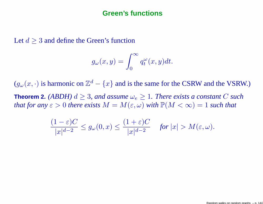
Let d ≥ 3 and define the Green’s function

gω(x, y) =

∫ ∞

0

qωt (x, y)dt.

(gω(x, ·) is harmonic onZd − x and is the same for the CSRW and the VSRW.)

Theorem 2. (ABDH)d ≥ 3, and assumeωe ≥ 1. There exists a constantC suchthat for anyε > 0 there existsM = M(ε, ω) with P(M < ∞) = 1 such that

(1 − ε)C

|x|d−2≤ gω(0, x) ≤

(1 + ε)C

|x|d−2for |x| > M(ε, ω).


Why are the CSRW and VSRW different ?

Recall the jump rates fromx to y are:

(1) ωxy for the VSRW,(2) ωxy/

∑z ωxz for the CSRW.

Consider a configuration like this, where black bonds haveωe ≈ 1 and the redbondx, y hasωxy = K ≫ 1.

The red bond acts as a ‘trap’. Both walks jump across the red bondO(K) timesbefore escaping. Since each jump takes timeO(1), the CSRW takes time0(K).Each jump takes the VSRW timeO(K−1), so the total time is onlyO(1).


Why may GB fail?

Consider a configuration like this:

The blue bond with0 < ωe << 1 attached to the black bond acts as a kind of‘battery’, and can hold the random walk for a long period.


Overview of proofs

1. The basic idea is to follow Kipnis-Varadhan and constructthe ‘corrector’χ(ω, x) : Ω × Z

d → Rd such that forP-a.a.ω

Mt = Yt − χ(ω, Yt) is aP 0ω-martingale.

Then one proves:

M(n)t = n−1/2Mnt ⇒ σWt, (1)

n−1/2χ(ω, Ynt) → 0, in P 0ω probability. (2)

2. A general CLTs for martingales (Helland, 1982) gives convergence in(1).

3. To control the corrector one needs something like:

limn→∞

max|x|≤n

χ(ω, x)

n= 0. (3)

In d ≥ 3 proving this requires upper bounds onqωt (x, y).


Heat kernel bounds – 1

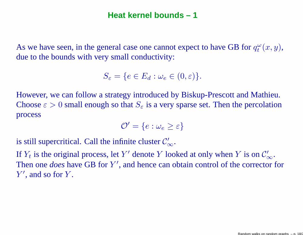
As we have seen, in the general case one cannot expect to have GB for qωt (x, y),

due to the bounds with very small conductivity:

Sε = e ∈ Ed : ωe ∈ (0, ε).

However, we can follow a strategy introduced by Biskup-Prescott and Mathieu.Chooseε > 0 small enough so thatSε is a very sparse set. Then the percolationprocess

O′ = e : ωe ≥ ε

is still supercritical. Call the infinite clusterC′∞.

If Yt is the original process, letY ′ denoteY looked at only whenY is onC′∞.

Then onedoeshave GB forY ′, and hence can obtain control of the corrector forY ′, and so forY .


Heat kernel bounds - 2

A general guide to proving heat kernel bounds is given by the following theorem.

Theorem B. (T. Delmotte, 1999). LetG = (V, E) be a (locally finite) graph, withdistanced(x, y). The following are equivalent:(a) The heat kernelqt(x, y) satisfies (GB).(b) G satisfiesVolume DoublingandPoincaré inequality: VD+PI.[ (c) Solutions of the heat equation onG satisfy a PHI. ]

Here (GB) means that ift ≥ 1 ∨ d(x, y)

exp(−c1d(x, y)2/t)

|B(x, c1t1/2)|≤ qt(x, y) ≤

exp(−c2d(x, y)2/t)

|B(x, c2t1/2)|.

Note that|B(x, t1/2| can be replaced byctd/2 if, as is the case onZd,

crd ≤ |(B(x, r)| ≤ c′rd.


VD and PI for graphs

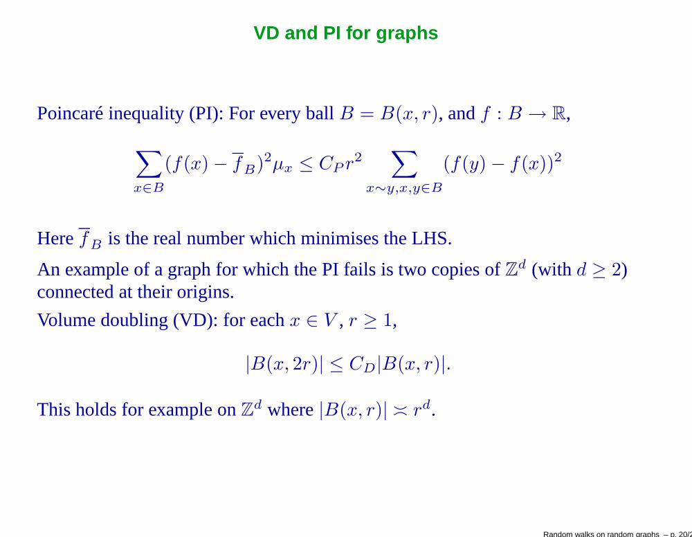
Poincaré inequality (PI): For every ballB = B(x, r), andf : B → R,

∑x∈B

(f(x) − fB)2µx ≤ CP r2∑

x∼y,x,y∈B

(f(y) − f(x))2

HerefB is the real number which minimises the LHS.

An example of a graph for which the PI fails is two copies ofZd (with d ≥ 2)

connected at their origins.

Volume doubling (VD): for eachx ∈ V , r ≥ 1,

|B(x, 2r)| ≤ CD|B(x, r)|.

This holds for example onZd where|B(x, r)| ≍ rd.


Heat kernel bounds - 3

Delmotte’s theorem was based on the characterization of PHIon manifolds due toGrigoryan and Saloffe-Coste. This in turn was ultimately based on work onMoser in the early 1960s.

In the random graph case, it has (so far) proved difficult to adapt Moser’smethods. But other techniques due to Nash can be used, and give a version ofTheorem B which holds for supercritical percolation clusters.

A similar approach also works in for the truncated clusterC′∞, and gives (GB) for

Y ′.

This then leads to good control of the correctorχ and hence to a FLCT for theVSRW.


CSRW

Once we have the QFCLT for the VSRWY it is easy to get it for the CSRWX .Set

At =

∫ t

0

µYsds,

and letτt be the inverse ofA. Then the CSRWX is given by

Xt = Yτt, t ≥ 0.

By the ergodic theorem

At/t → C = 2d E1ωe ∈ [1,∞],

soτt/t → C−1 ∈ [0, 1]. So we get the QFCLT forX , and the diffusivityσ2X is

positive if and only ifC < ∞, i.e. if and only if

Eωe < ∞.


CSRW: beyond the CLT

If Eωe = ∞ then we just have

X(n)t = n−1/2Xnt → 0.

The reason is thatX spends long periods in the ‘traps’, i.e. jumping across ‘redbonds’e = x, y with ωe ≫ 1.‘Fractional kinetic motion’ FK(α). Let d ≥ 1, W be BM(Rd) andξt be anindependent stable subordinator indexα ∈ (0, 1). Let Lt be the inverse ofξ:Lt = infs : ξs > t. Then the FK(α) is given by:

R(α)t = WLt

, t ≥ 0.

R is not Markov, moves like a BM, but has long periods of remaining constant.MB and J.Cerný: ifd ≥ 3, andP(ωe > t) ∼ t−α then

n−α/2Ynt ⇒ cR(α)t .


Fractional Kinetic motion


random walks on random graphs - university of british ...barlow/talks/iciam.pdf · random walks on...

Documents