HAL Id: halshs-01082996https://halshs.archives-ouvertes.fr/halshs-01082996v2

Preprint submitted on 21 Dec 2015

HAL is a multi-disciplinary open accessarchive for the deposit and dissemination of sci-entific research documents, whether they are pub-lished or not. The documents may come fromteaching and research institutions in France orabroad, or from public or private research centers.

L’archive ouverte pluridisciplinaire HAL, estdestinée au dépôt et à la diffusion de documentsscientifiques de niveau recherche, publiés ou non,émanant des établissements d’enseignement et derecherche français ou étrangers, des laboratoirespublics ou privés.

Ranking Distributions of an Ordinal AttributeNicolas Gravel, Brice Magdalou, Patrick Moyes

To cite this version:Nicolas Gravel, Brice Magdalou, Patrick Moyes. Ranking Distributions of an Ordinal Attribute. 2015.�halshs-01082996v2�

Working Papers / Documents de travail

WP 2014 - Nr 50

Ranking Distributions of an Ordinal Attribute

Nicolas GravelBrice Magdalou

Patrick Moyes

Ranking distributions of an ordinal attribute ∗

Nicolas Gravel†, Brice Magdalou‡and Patrick Moyes§

Keywords: ordinal, qualitative, health, inequality,

Hammond transfers, increments, dominance

JEL codes: C81, D63, I1, I3

December 13th 2015

Abstract

This paper establishes foundational equivalences between alternative

criteria for comparing distributions of an ordinally measurable attribute.

A first criterion is associated with the possibility of going from distribution

to the other by a finite sequence of two elementary operations: increments

of the attribute and Hammond transfers. The later transfers are like the

famous Pigou-Dalton ones, but without the requirement - that would be

senseless in an ordinal setting - that the "amount" transferred from the

"rich" to the "poor" is fixed. A second criterion is a new easy-to-use

statistical criterion associated to a specifically weighted recursion on the

cumulative density of the distribution function. A third criterion is that

resulting from the comparison of numerical values assigned to distributions

by a large class of additively separable social evaluation functions. Dual

versions of these criteria are also considered and alternative equivalence

results are established. Illustrations of the criteria are also provided.

1 Introduction

When can we say that a distribution of income among a collection of individuals

is more equal than another ? One of the greatest achievement of the modern

theory of inequality measurement is the demonstration, made by Hardy, Lit-

tlewood, and Polya (1952) and popularized among economists by Kolm (1969)

Atkinson (1970) Dasgupta, Sen, and Starrett (1973), Sen (1973) and Fields and

Fei (1978), that the following three answers to this question are equivalent :

∗This article is significant extension of a paper with the same title released as the AMSEworking paper no 2014-50. In preparing this extension, we have benefited greatly from the

detailed comments made by Ramses Abdul Naga on the earlier paper. He bears of course no

responsibility for any remaining deficiencies.†Aix-Marseille Univ. (Aix-Marseille School of Economics), CNRS & EHESS, Centre de la

Vieille Charité, 2, rue de la Charité, 13002, Marseille France.‡Université de Montpellier 1 & LAMETA, rue Raymond Dugrand, 34960 Montpellier,

France.§CNRS, GRETHA, Université Montesquieu (Bordeaux 4), Avenue Léon Duguit, 33 608

Pessac, France.

1

1) When one distribution has been obtained from the other by a finite se-

quence of Pigou-Dalton transfers.

2) When one distribution would be considered better than the other by all

utilitarian philosophers who assume that individuals convert income into utility

by the same increasing and concave function.

3) When the Lorenz curve associated to one distribution lies nowhere below,

and at least somewhere above, that of the other.

The equivalence of these three answers - often referred to as the Hardy-

Littlewood-Polya (HLP) theorem - is an important result because it ties together

three a priori distinct aspects of the process of inequality measurement.

The first one - contained in the Pigou-Dalton principle of transfers - is an

elementary transformation of the distribution of income that captures in a crisp

fashion the nature of the equalization process that is at stake. It provides a first,

immediately palatable, answer to the question raised above. A distribution is

more equal than another when it has been obtained from it by a finite sequence

of such "clearly equalizing" Pigou-Dalton transfers.

The second aspect of the process of inequality measurement identified by the

HLP theorem is the ethical principle underlying utilitarianism or, more gener-

ally, additively separable social evaluation. Attitude toward income inequality

is clearly an ethical matter. It is therefore of importance to identify the ethi-

cal principles that rationalize the notion of inequality reduction underlying the

Pigou-Dalton principle of transfers. While the HLP theorem points toward

utilitarianism or additively separable social evaluation as a source of such ra-

tionalization, it can be shown (see e.g. Gravel and Moyes (2013)) that such a

rationalization can also be obtained through a much more general class of social

evaluation functions.

The third aspect of the process of inequality measurement captured by the

HLP theorem is the empirically implementable criterion underlying Lorenz dom-

inance. It is, indeed, immensely useful to have an implementable criterion like

the Lorenz curve that enables one to check in an easy manner when one distrib-

ution dominates another. Comparisons of Lorenz curves have become a routine

exercise that is performed every day by thousands of researchers worldwide.

Moreover, compatibility with the Lorenz ranking of income distributions is now

considered to be a minimal requirement that any numerical index of income

inequality must satisfy. In this sense, the HLP theorem is, in the literal sense

of the word, a foundation to income inequality measurement.

The current paper is concerned with establishing analogous foundations to

the problem of comparing distributions of an ordinal or qualitative attribute

among a collection of individuals. The last fifteen years have witnessed indeed an

extensive use of data involving distributions of attributes such as access to basic

services, educational achievements, health outcomes, and self-declared happiness

to mention just a few. When performing normative comparisons of distributions

of such attributes, it is not uncommon for researchers to disregard the ordinal

measurability of the attribute and to treat it, just like income, as a variable

that can be "summed", or "transferred" across individuals. Examples of those

practices include Castelló-Clement and Doménech (2002) and Castelló-Clement

and Doménech (2008) (who discusses inequality indices on human capital) and

Pradhan, Sahn, and Younger (2003) (who decompose Theil indices applied to

the heights of under 36 month children interpreted as a measure of health).

Yet, following the influential contribution by Allison and Foster (2004), there

2

has been a growing concern by researchers of duly accounting for the ordinal

character of the numerical information conveyed by the indicators used in those

studies. Examples of studies that have taken such a care, and have explicitly

refused to use cardinal properties of the attribute when normatively evaluating

its distribution, include Abul-Naga and Yalcin (2008) and Apouey (2007).

A difficulty with the normative evaluation of distributions of an ordinal at-

tribute is that of defining an appropriate notion of inequality reduction in that

context. What does it mean indeed for an ordinal attribute to be "more equally

distributed" than another ? The notion of Pigou-Dalton transfer used to answer

this question in the case of a cardinally measurable attribute is of no clear rele-

vance for that purpose. For a Pigou-Dalton transfer is the operation by which an

individual transfers to someone endowed with a lower quantity of the attribute

a certain quantity of that attribute. Such a transfer is obviously meaningless if

the "quantity" of the attribute is ordinal. While ordinal measurability of the at-

tribute - provided that it is comparable across different individuals - enables one

to identify which of two individuals has "more" of the attribute than the other,

it does not enable one to quantify further the statement. It does not enable one

to talk about a "certain quantity" of the attribute that can be transferred across

individuals.

Some forty years ago, Peter J. Hammond (1976) has proposed, in the spe-

cific context of social choice theory, a so-called "minimal equity principle" that

was explicitly concerned with distributions involving an ordinally measurable

attribute. According to Hammond’s principle, a change in the distribution that

"reduces the gap" between two individuals endowed with different quantities of

the ordinal attribute is a good thing, irrespective of whether or not the "gain"

from the poor recipient is equal to the "loss" from the rich giver. A Pigou-Dalton

transfer is clearly a particular case of a Hammond transfer, that imposes on the

later the additional requirement that the amount given by the rich be equal to

the amount received by the poor. It seems to us that the purely ordinal nature

of Hammond transfers qualifies them as a highly plausible instances of "ordinal

inequality reduction". This paper identifies a normative dominance criterion and

a statistically implementable criterion that are each equivalent to the notion of

equalization underlying Hammond transfer. It does so in the specific, but empir-

ically important, case where the ordinal attribute can take only a finite number

different values. This finite case is somewhat specific indeed for discussing the

Hammond equity principle. For, as is well-known in social choice theory (see e.g.

D’Aspremont and Gevers (1977), D’Aspremont (1985), Sen (1977)), the Ham-

mond equity principle is closely related to "Maximin" or "Leximin" types of

criteria that rank distributions of an ordinal attribute on the basis of the small-

est quantity of the attribute. Bosmans and Ooghe (2013) have even shown that

any anonymous, continuous, and Pareto-inclusive transitive ranking of all vec-

tors of R that is sensitive to Hammond transfer must be the Maximin criterionthat compares such vectors on the sole basis of the size of their smallest compo-

nent. As shall be seen in this paper, this apparently tight connection between

Maximin or Leximin principles and Hammond transfers becomes significantly

looser when attention is restricted to distributions of an attribute that can take

finitely many different values.

As for the normative principle, we stick to the tradition of comparing distri-

butions of the attribute by means of an additively separable social evaluation

function. Each attribute quantity is thus assigned a numerical value by some

3

function, and alternative distributions of attributes are compared on the basis

of the sum - taken over all individuals - of these values. While this normative

approach can be considered utilitarian (if the function that assigns a value to the

attribute is interpreted to be a "utility" function), it does not need to. One could

also interpret the function more generally as an advantage function reflecting

the value assigned to each individual attribute quantity by the "social planner"

or the "ethicist". It is also possible to justify axiomatically this additively sepa-

rable normative evaluation in a non-welfarist setting (see e.g. Gravel, Marchant,

and Sen (2011)). As the ordinal attribute (health indicator, education, access to

basic services) is considered to be a good thing to the individual, it is assumed

that the advantage function is increasing with respect to the attribute. We show

in this paper that, in order for a ranking of distributions based on an additively

separable social evaluation function to be sensitive to Hammond transfers, it is

necessary and sufficient for the advantage function to satisfy a somewhat strong

"concavity" property. Specifically, any increase in the quantity of the attribute

obtained from some initial level must increase the advantage more than any

increase in the attribute taking place at some higher level of the attribute, no

matter what the later increase is. Because of this result, we therefore consider

the ranking of distributions of the ordinal attribute that coincides with the una-

nimity of all additively separable rankings who use an advantage function that

satisfies this property.

The empirical implementable criterion that we consider is, to the very best

of our knowledge, a new one. Its construction is based on a curve that we

call the +-curve, by reference to the Hammond principle of transfer to which

it is, as it turns out, closely related. The + curve is defined recursively as

follows. It starts by assigning to the lowest possible quantity of the ordinal

attribute the fraction of the population that are endowed with this quantity.

For this lowest category, this number is nothing else than the relative frequency

of the category or, equivalently for the lowest category, its cumulative frequency.

One then proceeds recursively, for any quantity of the attribute strictly larger

than this smallest quantity, by adding together the relative frequency of the

population endowed with this quantity of the attribute and twice the value

assigned by the curve to the immediately preceding category. The innovation of

this curve lies precisely in its addition, to any fraction of the population falling

in some category, of twice the value assigned by the curve to the immediately

preceding category. This (doubly) larger weight given to the preceding category

as compared to any given category reflects, of course, the somewhat strong

redistributive flavour of the Hammond’s equity principle. The criterion that we

propose, and that we call +-dominance, is for the dominating distribution to

have a +-curve nowhere above and somewhere below that of the dominated

one. As illustrated below, the construction of these curves, and the resulting

implementation of the criterion, is easy.

This paper provides some justification for the use of such a+-curve. It does

so by proving that the fact of having a distribution of an ordinal attribute that

+-dominates another is equivalent to the possibility of going from the latter to

the former by a finite sequence of Hammond transfers and/or increments of the

attribute. The paper also shows that the +-dominance criterion coincides with

the unanimity of all additively separable aggregation of advantage functions that

use an advantage function that is strongly decreasingly increasing in the sense

given above.

4

While these results justify comparing distributions of an ordinal attribute

on the basis of +- dominance, they do not readily lead to a definition of what

it means for a distribution or an ordinal attribute to be "more equal" than

another. In effect, + dominance combines together both Hammond transfers

and increments. While the former transformation is a plausible candidate for a

definition of an inequality reduction in an ordinal setting, the later is not. Could

one identify an operational criterion that coincides with Hammond transfers

only and that could serve, as a result, as an operational definition of inequality

reduction in an ordinal setting ?

A parallel with the classical cardinal case can be useful for understanding

this point. In this classical setting, it is well-known that if two distributions of

an attribute have the same sum (or the same mean), then the Lorenz domi-

nation of one distribution by the other is equivalent to the possibility of going

from the dominated distribution to the dominating one by a finite sequence

of Pigou-Dalton transfers. For distributions with the same mean therefore, in-

equality reduction in the sense of Pigou-Dalton transfers is equivalent to Lorenz

domination. If there was a meaningful analogue - in the ordinal setting - to

the requirement that two distributions have the "same mean", one could think

at paralleling - for that analogue - the standard approach and at identifying

+ domination with Hammond transfers only. Unfortunately there is no such

meaningful analogue to the mean in the ordinal setting. However, there is an-

other (less well-known) path taken from the theory of majorization (see e.g.

Marshall, Olkin, and Arnold (2011)) that can be followed to handle that is-

sue. From that theory (see Marshall, Olkin, and Arnold (2011) (chapter 1,

p. 13, equation (14)), it can be noticed that Lorenz dominance between two

distributions of a cardinal attribute with the same sum is nothing else than

the intersection of two independent majorization quasi-orderings that do not

assume anything about the "sum" of the attribute. The first one, called subma-

jorization by Marshall, Olkin, and Arnold (2011), defines a distribution to be

better than a distribution 0 if, for any rank , the sum of income of the individ-uals weakly richer than is weakly smaller in than in 0. The second criterion,called supermajorization by Marshall, Olkin, and Arnold (2011), corresponds

to the more usual generalized Lorenz domination criterion (see e.g. Shorrocks

(1983)) according to which distribution is better than distribution 0 if thesum of the lowest incomes is weakly larger in than in 0 no matter what is. In this paper, we parallel the route taken by Marshall, Olkin, and Arnold

(2011) by exploring a dual domination criterion based on the − curve of adistribution of an ordinal attribute. This curve is constructed just like the +

one but, contrary to the later, it starts from "above" (that is from the highest

ordinal category) rather than from "below", and iteratively cumulate the (dis-

crete) survival function rather than the (discrete) cumulative function. We then

establish that this notion of − domination coincides with the possibility of go-ing from the dominated distribution to the dominating one by a finite sequence

of either Hammond transfers and/or decrements. As for the submajorization

and supermajorization criteria in the classical cardinal setting, the ranking of

distributions generated by the intersection of the two domination criteria +

and − could serve as a plausible instance of a clear inequality reduction inan ordinal setting. Indeed, as established in this paper, any finite sequence of

Hammond transfers would be recorded as an improvement by this intersection

ranking.

5

While we do not have available a proof of the converse implication, we do

have results that lead somewhat toward it. One of theses results is the equiva-

lence that we establish between the intersection of the + and the − dom-inance criteria on the one hand, and the intersection of all rankings produced

by additively separable social evaluation functions that use a strongly concave

- in the sense alluded to above - but not necessarily monotone individual ad-

vantage function on the other. Another such a result is the examination of the

two + and − criteria that we provide when the finite grid used to definethe categories is refined. Indeed, every criterion considered in this paper de-

pends upon the finite grid of attribute values that is considered. What happens

to the criterion when the grid thus considered is refined ? We show in this

paper that there exists a level of grid refinement above which the + dom-

ination criterion coincides with the Leximin ranking of the two distributions.

Similarly we indicate that there exists a level of grid refinement above which

the − domination criterion coincides with the (anti) Leximax ranking of thosetwo distributions. Notice that these results are consistent with those obtained

in classical social choice theory (see Hammond (1976), Deschamps and Gevers

(1978), D’Aspremont and Gevers (1977), Sen (1977)). The Leximin criterion

can be viewed as the limit of the + criterion when the number of different

categories of the attribute becomes arbitrarily large. Similarly the anti Leximax

criterion can be viewed as the limit of the − criterion when the number ofdifferent categories becomes large. It follows of course from these two remarks

that the intersection of the anti Leximax and the Leximin criteria is the limit of

the intersection of the + and the − criteria when the number of categoriesbecomes large. Since, as proved in Gravel, Magdalou, and Moyes (2015), the in-

tersection of the anti-Leximax and the Leximin criteria is the transitive closure

of the binary relation "is obtained from by a Hammond transfer" applied to all

vectors in a closed and convex subset of R, we view this result as a suggestiveevidence that the possibility of going from a distribution to a distribution

by a finite sequence of Hammond transfers is closely related to the dominance

of by by both the + and the − criterion.The plan of the rest of the paper is as follows. The next section introduces

the notation, discusses the general problem of comparing distributions of an

ordinal attribute, and presents the normative dominance notions, the elemen-

tary transformations (Hammond transfers and increments/decrements) and the

implementation criteria ( curves) in the specific setting where the ordinal at-

tribute can take finitely many different values. The main results identifying the

elementary transformations underlying the + and the −curves are statedand proved in the fourth section. The fourth section discusses the connection

between the discrete setting in which the analysis is conducted and the classical

social choice one in which the Hammond equity principle has been originally

proposed and establishes the results mentioned above on the behavior of the

+ (and the −) criterion when the number of different categories is enlarged.The fifth section illustrates the usefulness of the criteria for comparing distri-

butions of Body Mass Index categories among genders in France, UK and the

US. The sixth section concludes.

6

2 Three perspectives for comparing distributions

of an ordinal attribute

2.1 Normative evaluation

We consider distributions of an ordinal attribute between a given number - say

- of individuals, indexed by . As is standard in distributional analysis since at

least Dalton (1920), distributions of the attribute between a varying number of

individuals can be compared by means of the principle of population replication

(replicating a distribution any number of times is a matter of social indifference).

We assume that there are (with ≥ 3) different values that the ordinal

attribute can take. These values, which can be interpreted as "categories" (e.g.

"being gravely ill", "being mildly ill", "being in perfect health"), are indexed by

. We denote by C = {1 } the set of these categories, assumed to be orderedfrom worst (e.g. being gravely ill) to the best (e.g. being in perfect health).

The fact that the attribute is ordinal means that the integers 1 assigned

to the different categories have no particular significance other than ordering

the categories from the worst to the best. Hence, any comparative statement

made on two distributions in which the attribute quantity is measured by the

list of numbers {1 } would be unaffected if this list was replaced by thelist (1) () generated by any strictly increasing real valued function

admitting as its subdomain.

A society = (1 ) ∈ C is a particular assignment of these categoriesto the individuals, where is the category assigned to in society . For any

society , and every category , one can define the number of individuals

who, in , falls in category by:

= #{ ∈ {1 } : = }

We of course notice thatP=1

= for every society . If one adopts an anony-

mous perspective according to which "the names of the individuals do not mat-

ter", then the integers (for = 1 ) summarize all the ethically relevant

information about society . The current paper adopts this anonymous perspec-

tive and examines, more specifically, the family of additively separable rankings

º of societies in C that can be defined, for any two societies and 0 in C,by:

º 0 ⇐⇒X

=1

≥X

=1

0 (1)

for some list of real numbers (for = 1 ). These numbers can of

course be seen as numerical evaluations of the corresponding categories (in which

case we could require them to satisfy 1 ≤ ≤ ). These valuations may

reflect subjective utility (if a utilitarian perspective is adopted) or a non-welfarist

appraisal made by the social planner of the fact, for someone, to falling in

the different categories to which these numbers are assigned. If such a non-

welfarist perspective is adopted, the specific additive form of the numerical

representation (1) of the social ordering can be axiomatically justified (see e.g.

Gravel, Marchant, and Sen (2011)).

7

The ordinal interpretation of the categories suggests that some care be taken

in avoiding the normative evaluation exercise to be unduly sensitive to particular

choices of the numbers (for = 1 ). A standard way to exert such a

care is to require the unanimity of evaluation over a wide class of such lists of

numbers. This underlies the following general definition of normative dominance.

Definition 1 For any two societies and 0 in C, we say that normativelydominates 0 for a family A ⊂ R of evaluations of the categories, denoted

ºA 0, if one has:X

=1

≥X

=1

0

for all (1 ) ∈ A.

The elementary transformations and implementable criteria that will be dis-

cussed in the next two subsections will be shown to be somewhat tightly as-

sociated with specific - but somewhat large - families of evaluations of the

categories.

2.2 Elementary transformations

The definition of these transformations lies at the very heart of the problem of

comparing alternative distributions of an ordinally measured attribute. Indeed,

these transformations are intended to capture in a crisp and concise fashion one’s

intuition about the meaning of "equalizing" or "gaining in efficiency" (among

others). In defining these transformation, it is important to make sure that they

use only ordinal property of the attribute. In this paper, we discuss three such

transformations.

The first of them - the increment - is hardly new. It captures the intuitive

idea - somewhat related to efficiency - that giving to someone - up to a per-

mutation thanks to anonymity - additional quantities of the ordinal attribute

without reducing - up to a permutation - the quantity of attribute of the others

is a good thing. We actually formulate this principle in the following minimalist

fashion.

Definition 2 (Increment) We say that society has been obtained from society

0 by means of an increment, if there exist ∈ {1 − 1} such that:

= 0 ∀ 6= + 1 ; (2)

= 0 − 1 ; +1 =

0+1 + 1 (3)

In words, society has been obtained from society 0 by an increment ifthe move from 0 to is the sole result of the move of one individual from a

category to the immediately superior category +1. The notion of increment

is the minimal formulation of the idea that increasing (up to a permutation of

individuals) the quantity of the attribute for someone is a good thing if it does

not reduce the attribute of others. In a somewhat reverse fashion, we can also

introduce the notion of a decrement as follows.

8

Definition 3 (Decrement) We say that society has been obtained from society

0 by means of a decrement, if there exist ∈ {1 − 1} such that:

= 0 ∀ 6= + 1 ; (4)

= 0 + 1 ;

+1 =

0+1 − 1 (5)

In words, society has been obtained from society 0 by an decrement if themove from 0 to is the sole result of the move of one individual from a category+1 to the immediately inferior category . A decrement would be a normatively

improving operation if the the categories {1 } were decreasingly ordered orif the ordinal attribute was considered to be a "bad", rather than a "good". The

following obvious, and therefore unproved, remark recalls that a decrement is

nothing else than the converse of an increment.

Remark 1 Society has been obtained from society 0 by means of a decre-ment if and only if society 0 has been obtained from society by means of an

increment.

The third elementary transformation considered in this paper is that under-

lying the equity principle put forth by Peter J. Hammond (1976) some forty

years ago. It reflects an appealing - if not strong - notion of aversion to inequal-

ity in contexts where the distributed attribute - taken to be utility in Hammond

(1976) - is ordinal. This principle considers that a reduction in someone’s en-

dowment of the attribute compensated by an increase in the endowment of some

other person is a good thing if the looser remains, after the loss, better off than

the winner. While a reduction in someone’s endowment that is compensated by

an increase in that of someone else may be viewed as the result of a "trans-

fer" of attribute between the two persons, it is worth noticing that, contrary

to what is the case with standard Pigou-Dalton transfers, the "quantity" of the

attribute given by the donor needs not be equal to that received by the recipi-

ent. A Hammond transfer may involve taking "a lot" of attribute away from a

"rich" person in exchange of giving "just a little bit" to a poorer one. It may,

conversely, entail the transformation of a "small" quantity" taken from the rich

into a "large" one given to the poor. As the comparisons of gains and loss of an

ordinal attribute is meaningless, the Hammond transfer may be viewed as the

natural analogue, in the ordinal setting, of the Pigou-Dalton transfer used in

the cardinal one. The precise definition we give of a Hammond transfer is the

following.

Definition 4 (Hammond’s transfer) We say that society is obtained from

society 0 by means of a Hammond’s (progressive) transfer, if there exist fourcategories 1 ≤ ≤ ≤ such that:

= 0 ∀ 6= ; (6a)

= 0 − 1 ; =

0 + 1 ; (6b)

= 0 + 1;

=

0 − 1 (6c)

9

It should be noticed that a Pigou-Dalton transfer is, in the current discrete

setting, nothing else than a Hammond transfer for which the indices , and

of Definition 4 satisfy the additional condition that − = − (a given -

by − - quantity of the attribute is transferred). This additional condition has

little meaning given the ordinal nature of the attribute. But it could certainly

be imposed if, as in the literature on discrete first and second order dominance

(see e.g. Fishburn and Lavalle (1995) or Chakravarty and Zoli (2012)), the gap

between any two adjacent categories was believed to be meaningfully constant.

2.3 Implementation criteria

Three implementation criteria are considered in this paper. The first one - first

order stochastic dominance - is standard in the literature. Its formal definition in

the current setting makes use of the cumulative distribution function associated

to a society , that is denoted, for every ∈ C, by (; ) and that is defined,

for = 1 , by:

(; ) =

X=1

(7)

Using this definition, one can define first order dominance as follows.

Definition 5 (1st order dominance) We say that society first order dominates

society 0, which we write º1 0, if and only if: (; ) ≤ (; 0) ∀ = 1 2 (8)

(remembering of course that (; ) =P

=1 = 1 for any society ).

The second implementation criterion examined in this paper is based on the

following + curve (defined for any society and any ∈ {1 }):

+(; ) =

X=1

¡2−

¢ (9)

A few remarks can be made about this curve.

First, it verifies:

+(1; ) = (1; ) (10)

and:

+(; ) =

−1X=1

¡2−−1

¢ (; ) + (; ) ∀ = 2 3 (11)

The different values of +(·; ) are therefore nested. Moreover, for any =

2 3 , we have:

+(; ) = 2+(− 1; ) + (; )− (− 1; ) = 2+(− 1; ) + (12)

Hence, by successive decomposition, one obtains, for all = 2 3 :

+(; ) =¡2¢+(− ; ) +

−1X=0

¡2¢ −

∀ = 1 2 − 1 (13)

This curve gives rise to the following notion of dominance - called + domi-

nance.

10

Definition 6 (+ dominance) We say that society +-dominates society 0,which we write º+ 0, if and only if:

+(; ) ≤ +(; 0) ∀ = 1 2 (14)

A few additional remarks are in order on the + curves and the +-

dominance criterion to which they give rise. The definition of the + curve

as per expression (11) makes clear that first order stochastic dominance implies

+ dominance. In plain English, +(; ) is a (specifically) weighted sum of

the fractions of the population in that are in weakly worse categories than .

The weight assigned to the fraction of the population in category (for )

in that sum is 2−. Hence the weights are (somewhat strongly) decreasing withrespect to the categories. A nice feature of the + curve - that appears strik-

ingly in formula (12) - is its recursive construction, that is quite similar to that

underlying the cumulative distribution curve. The cumulative distribution

can indeed be defined recursively by:

(1; ) = 1 (15)

and, for = 2 , by:

(; ) = (− 1; ) + (16)

The recursion that defines + starts just in the same way than as in (15) with:

+(1; ) = 1

but has the iteration formula (16) replaced by:

+(; ) = 2+(− 1; ) +

The last implementation criterion examined in this paper is somewhat dual to

+ dominance. Its formal definition makes use of the complementary cumulative

distribution function - also known as the survival function - associated to a

society , that is denoted, for every ∈ C, by (; ) and that is defined by:

(; ) = 1− ( ) (17)

=

X=+1

for = 1 − 1 and, (18)

= 0 for = (19)

Hence (; ) is the fraction of the population in who is in a strictly better

category than . For technical reasons in some of the proofs below, we find useful

to extend the domain of definition of (; ) from C = {1 } to {0 } andto set (0; ) = 1. With this notation, one can define the last implementation

criterion examined in this paper by means of the following − curve defined,for any society and any ∈ {1 }, by:

−(; ) =X

=+1

¡2−−1

¢ for = 1 − 1 (20)

11

and:

−(; ) = 0 (21)

This curve is thus constructed under exactly the same recursive principle than

the + one, but starting with the highest category, and iterating with the

complementary cumulative distribution function rather than with the standard

cumulative one. The − curves therefore starts at category − 1:−( − 1; ) = ( − 1; ) = (22)

and satisfies:

−(; ) =X

=+1

¡2−−1

¢ (; ) + (; ) ∀ = 1 2 − 1 (23)

so that the different values of −(·; ) are nested starting from above and goingbelow. Moreover, for any = 1 2 − 2 we have:−(; ) = 2−(+ 1; ) + (; )− (+ 1; ) = 2−(+ 1; ) + (24)

Hence, just as in expression (13) above, one obtains, by successive decomposi-

tion, for all = 1 2 − 2:

−(; ) =¡2−

¢−( − ; ) +

X=+1

¡2−−1

¢ −

∀ = + 1 − 1

(25)

This curve gives rise to the following notion of dominance.

Definition 7 (− dominance) We say that society −-dominates society 0,which we write º− 0, if and only if:

−(; ) ≤ −(; 0) ∀ = 1 2 (26)

As illustrated in section 5, these two curves, constructed recursively from

the cumulative and complementary cumulative distribution functions thanks to

formula (12) and (24), are easy to use and draw. As will also be seen in the

next section, the two dominance criteria that they generate provide exact diag-

nostic test of the possibility of moving from the dominated distribution to the

dominating one by Hammond transfers and increment (for + dominance) or

decrements (for + dominance). Moreover, the additional criterion provided by

the intersection of − and + dominance - that we referred to as -dominance

- will turn out to appear tightly related to the notion of equalization contained

in the Hammond principle of transfers. For future reference, we define formally

this notion of dominance as follows.

Definition 8 ( dominance) We say that society -dominates society 0,which we write º 0, if and only if one has both º+ 0 and º− 0.

We end this section by providing links between some of these notions of

implementable dominance. Specifically, we show that first order dominance of

a society 0 by a society entails the + dominance of 0 by and the −

dominance of society by 0. As for all formal results of this paper, the proofof those results are gathered in the Appendix.

Proposition 1 Let and 0 ∈ C. Then º1 0 =⇒ º+ 0 ∧ 0 º−

12

3 Equivalence results

In this section, we provide a few theorems that connect together normative

dominance - as per definition 1 - over specific classes of collections of numbers

1 on the one hand and, on the other, specific implementable dominance

criteria as well as the possibility of going from the dominated to the dominating

distribution by appropriate elementary transformations of the distributions.

We start by stating the following technical result, proved in the Appendix,

that establishes an important decomposition property of the additively separable

criterion underlying the notion of normative dominance favoured in this paper.

Lemma 1 For any ∈ C and any conceivable collection of numbers (1 ) ∈R, one has:

1

X=1

= −−1X=1

(; ) [+1 − ] (27)

or equivalently:

1

X=1

= 1 +

−1X=1

(; ) [+1 − ] (28)

Moreover, for all = 2 3 − 1, one has:

1

X=1

= −−1X=1

(; ) [+1 − ] +

−1X=

(; ) [+1 − ] (29)

Endowed with this result, we start with the notions of increment and decre-

ment, as these elementary transformations can be appraised by normative dom-

inance. Indeed, suppose that we compare alternative societies on the basis of

a criterion that can be numerically represented by expression (1) for some list

1 of real numbers. A first question that arises is: what properties must

these numbers satisfy for a criterion numerically represented as per (1) to con-

sider an increment (a decrement) as a definite social improvement? It should

come as no surprise that the answer to this question is for the numbers to

belong to the two following sets:

A+1 = {(1 ) ∈ R : 1 ≤ ≤ }and

A−1 = {(1 ) ∈ R : 1 ≥ ≥ }The set A+1 is indeed the largest set of valuations of the categories over whichnormative dominance (as per definition 1) is consistent with the idea that the

"welfare" or the "advantage" associated to the categories by the social planner

be increasing with respect to them. It is clear that any criterion that writes as

per (1) for a list (1 ) of numbers in the set A+1 will consider an incrementas a normative improvement. Similarly, the set A−1 is the largest collection of

lists of numbers that are consistent with the idea that the social valuation

of the categories is decreasing (rather than increasing) with respect to those.

Any additively separable normative judgement made by a criterion that can be

represented as per (1) for a list (1 ) of numbers in A−1 will consider a

decrement to be a good thing (or an increment to be a bad one).

The following two propositions establish this formally.

13

Proposition 2 Let be a society that has been obtained from 0 by an incre-ment as per definition 2. Then ºA 0 if and only if A = A+1 .

Proposition 3 Let be a society that has been obtained from 0 by an decre-ment as per definition 3. Then ºA 0 if and only if A = A−1 .

We now use these propositions to establish the following two theorems.

The first theorem has been known for quite a long time (see e.g. Lehmann

(1955) or Quirk and Saposnik (1962)). We nonetheless provide a proof of part

of it for completeness and for later use in the proof of the important Theorem

3 below.

Theorem 1 For any two societies and 0 ∈ C, the following three statementsare equivalent:

(a) is obtained from 0 by means of a finite sequence of increments,(b) ºA+

10,

(c) º1 0.

The second theorem is dual to the previous one. It links decrements to nor-

mative dominance over the set A−1 of valuations of the categories on the onehand and (anti) stochastic dominance on the other. The formal statement of

this theorem - whose proof, similar to that of theorem 1, is left to the reader -

is as follows.

Theorem 2 For any two societies and 0 ∈ C, the following three statementsare equivalent:

(a) is obtained from 0 by means of a finite sequence of decrements,(b) ºA−1 0,(c) 0 º1 .

We now turn to Hammond transfers. In a parallel fashion to what has been

established before propositions 2 and 3, we first ask under what conditions on

the set A of valuations of categories is normative dominance - as per definition1 - sensitive to Hammond transfers (as per definition 4). It turns out that the

answer to this question involves the following subset AH of R

AH =©(1 ) ∈ R | ( − ) ≥ ( − ) for 1 ≤ ≤ ≤

ª(30)

In words, AH contains all lists of categories’ evaluations that are "strongly

concave" with respect to these categories in the sense that the "utility" or

"advantage" gain of moving from one category to a better one is always larger

when done from categories in the bottom part of the scale than when done

in the upper part of it. The following proposition - proved in the Appendix

- establishes that the set AH of categories’ valuation is indeed the largest one

over which normative dominance (as per Definition 1) considers favorably the

notion of equalization underlying Hammond transfer.

14

Proposition 4 Let 0 ∈ C, and assume that is obtained from 0 by meansof a Hammond transfer. Then ºA 0 if and only if A = AH.

The intuition that the set AH captures a "strong concavity" property is,

perhaps, better seen through the following proposition, also proved in the Ap-

pendix, which establishes that AH contains all lists of categories’ valuations

that are "single-peaked" in the sense of admitting a largest value before which

they are increasing at a (strongly) decreasing rate and after which they are

decreasing at a (strongly) increasing rate.

Proposition 5 A list (1 ) of real numbers belongs to AH if and only

if there exists a ∈ {1 } such that (+1 − ) ≥ ( − +1) for all =

1 2 −1 (if any) and (0+1−0) ≤ (0−), for all 0 = +1 −1(if any).

Two particular "peaks" among those identified in Proposition 5 are of partic-

ular importance. One is when = so that the numbers 1 are increasing

(at a strongly decreasing rate) with respect to the categories. In this case, the

elements of AH are also in A+1 , and we denote by A+H = AH∩A+1 this set ofincreasing and strongly concave valuations of the categories. We then have the

following immediate (and therefore unproved) corollary of Proposition 5 (ap-

plied to = ).

Lemma 2 A list of real numbers (1 ) satisfies +1 − ≥ − +1for all ∈ {1 − 1} if and only if it belongs to A+H.

The other extreme of the possible peaks identified in Proposition 5 corre-

sponds to the case where = 1 so that the numbers 1 are decreasing

(at a strongly increasing rate) with respect to the categories. In this case, the

elements of AH are also in A−1 , and we denote by A−H = AH∩A−1 this subset ofthe set of all strongly concave valuations of the categories that are also decreas-

ing with respect to these categories. We then have the following also immediate

(and unproved) corollary of Proposition 5 (applied to = 1).

Lemma 3 A list of real numbers (1 ) satisfies +1− ≤ −1 forall ∈ {1 − 1} if and only if it belongs to A−H.

We now turn to the main result of this paper. This result states that +

dominance is the implementable test that enables one to check if one distribution

of an ordinal attribute is obtained from another by a finite sequence of either

Hammond transfers or increments. The formal statement of this result is as

follows.

Theorem 3 For any societies and 0 ∈ C, the following three statements areequivalent:

(a) is obtained from 0 by means of a finite sequence of Hammond’s transfersand/or increments,

(b) ºA+H0,

(c) º+ 0.

15

While a detailed proof of the equivalence of the three statements of Theo-

rem 3 is provided in the Appendix, it may be useful to sketch here the main

arguments. The fact that statement (a) implies statement (b) is an immediate

consequence of Propositions 2 and 4. These propositions indicate indeed that

normative dominance as per definition 1 over the set of categories’ valuations

A+H is sensitive to Hammond transfers and increments. The proof that statement(b) implies statement (c) amounts to verifying that any list of real numbers

(1 ) defined, for any ∈ {1 }, by:

= −(2−) for = 1 (31)

= 0 for ∈ {+ 1 } (32)

belongs to the set A+H. Indeed, it is apparent from expression (9) that verifying

the inequality:X

=1

≥

X=1

0

for any list (1 ) of real numbers defined as per (31) and (32) for any

is equivalent to the + dominance of 0 by . As, by definition of ºA+H,

inequality (1) holds for all (1 ) in the set A+H, it must hold in particularfor those (1

) defined as per (31) and (32) for any . The most difficult

proof that statement (c) implies statement (a) is obtained by first noting that

if º1 0 holds, then the possibility of going from 0 to by a finite sequence

of increments is an immediate consequence of Theorem 2. The proof is then

constructed under the assumption that º+ 0, but that does not dominate0 by first order dominance. Hence there must be some category at which thetwo cumulative density functions associated to and 0 "cross". We show that,in that case, one can make a Hammond transfer "above" the first category for

which this crossing occurs in such a way that the new society obtained after the

Hammond transfer remains dominated by as per the + dominance criterion.

We also show that this Hammond transfer "bring to naught" at least one of

the strict inequalities that distinguish ( ) from ( 0). Hence if the finaldistribution is not reached after this first transfer, then one can reapply the

same procedure again and again as many times as required to reach . As the

number of inequalities that distinguish ( ) from ( 0) is finite, this provethe implication.

We now state a theorem (proved in the appendix) that is the mirror image

of Theorem 3, but with increments replaced by decrements, the quasi-ordering

ºA+Hreplaced by ºA−H and the + dominance criterion replaced by the −

dominance one.

Theorem 4 For all societies and 0 ∈ C, the following three statements areequivalent:

(a) is obtained from 0 by means of a finite sequence of Hammond’s transfersand/or decrements,

(b) ºA−H 0,(c) º− 0.

Theorems 3 and 4 show that the + and − dominance criteria provide ex-act diagnostic tools of the possibility of going from the dominated society to the

16

dominating one by a finite sequence of Hammond transfers and increments and

Hammond transfers and decrements respectively. What about identifying the

possibility of going from a society to another by equalizing Hammond transfers

only ? It follows clearly from Theorems 3 and 4 that if this possibility exists

between two societies, then the society from which these transfers originate is

dominated by the society to which these transfers lead by both the + and

the − dominance criteria or, equivalently (Definition 8) by the dominance

criterion. Unfortunately, we do not have at our disposal a proof of the converse

implication that the dominance of a society by another as per the dominance

criterion entails the possibility of going from the dominated society to the dom-

inating one by a finite sequence of transfers only. Yet, it happens that that the

criterion of dominance is equivalent to additive normative dominance over

the class AH of ordered lists of real numbers. The following theorem describes

all the relations between Hammond transfers and the relevant normative and

implementable criteria that we are aware of.

Theorem 5 Consider any two societies and 0 ∈ C, and the following threestatements:

(a) is obtained from 0 by means of a finite sequence of Hammond’s transfers(b) ºA−H 0,(c) º 0.Then, statement (a) implies statement (b) and statement (b) and (c) are equiv-

alent.

4 Sensitivity of the criteria to the grid of cate-

gories.

As is well-known in classical social choice theory (see e.g. Hammond (1976),

Hammond (1976), Deschamps and Gevers (1978), D’Aspremont and Gevers

(1977) and Sen (1977)) Hammond transfers, when combined with the "Pareto

principle", is somewhat related with the lexicographic extension of the Maximin

(Leximin for short) criterion for ranking various ordered lists of numbers. For

example, Theorem 4.17 in Blackorby, Bossert, and Donaldson (2005) (ch. 4;

p. 123) states that the Leximin criterion is the only complete, reflexive, transi-

tive, monotonically increasing and anonymous ranking of R that is sensitive toHammond transfers. In the same vein, Bosmans and Ooghe (2013) and Miyag-

ishima, Bosmans, and Ooghe (2014) have shown that the Maximin criterion is

the only continuous and Pareto consistent reflexive and transitive ranking of R

that is consistent with Hammond transfers. Since the + dominance criterion

coincides, by Theorem 3, with the possibility of going from the dominated so-

ciety to the dominating one by a finite sequence of Hammond transfers and/or

increments - which are nothing else than anonymous Pareto improvements - it

is of interest to understand the connection between the + dominance criterion

and the Leximin one.

We start by defining the latter criterion in the current setting as follows.

Definition 9 Given two societies 0 ∈ C, we say that dominates 0 ac-cording to the Leximin, which we write º 0, if and only if there exists ∈ C,

17

such that 0 and = 0 for all ∈ C such that 1 ≤ (if there are

any such ).

It is clear (and well-known) that the Leximin criterion provides a complete

ranking of all lists of real numbers. The following proposition establishes that

the quasi-ordering º+ is a strict subrelation of º 0

Proposition 6 Assume that 2. Then, for any two societies and 0 ∈ C, º+ 0 =⇒ º 0, but the converse is false.

A key difference between the current framework and that considered in clas-

sical social choice theory is of course the discrete nature of the former. In the

framework considered here, the rankings are defined on C which can be viewedas a finite subset of N. In classical social choice theory, the criteria are takento be defined on the set R of all ordered lists of real numbers so that theattributes’ quantities are free to vary continuously.

In order to connect the two frameworks, we find useful to examine what

happens to the + criterion when the finite grid over which it is defined is

refined. As it turns out, for a suitably large level of grid refinement, the +

criterion becomes indistinguishable from the Leximin. There are obviously many

ways by which a given finite grid can be refined. In this section, we consider the

following notion of -refinement of the grid C = {1 2 }, for = 0 1

Definition 10 The -refinement of the grid C = {1 2 } for = 0 1 isthe set C() defined by:

C() = ©2 : = 1 2 (2)ª (33)

or, equivalently,

C() =½1

22

23

2

(2)

2

¾ (34)

Notice that C(0) = C so that the initial grid corresponds to a "zero" re-finement. The grid becomes obviously finer as increases, and it is clear that

C() ⊂ C(+1) for all = 0 . Hence, if the society (1 2 ) ∈ C, it alsobelongs to C() for all ∈ N. We also remark that the finite set C() tends tothe continuous interval ]0 ] as tends to infinity.

For any society , and any real number in the interval [0 ], we denote by

( ) the (possibly null) number of individuals in whose attribute takes the

value in the grid C() defined by:

( ) = # { ∈ {1 2 } : = }

We observe that, for any = 0 1 and society ∈ C(), one has:

( ) = 0 for all ∈ C() (35)

and, since C() ⊂ C(+ 1):

( + 1) = ( ) (36)

18

for all ∈ C(). Using these numbers () and applying the definition of the+ curve provided by Equation (9) to the grid C() enable one to define the-refinement of the + curve, denoted +

, as follows (for any ∈ C())

+ (0; ) = 0

and:

+

µ

2;

¶=1

X=1

¡2−

¢µ

2

¶ ∀ = 1 2 (2) (37)

We are now ready to define the notion of + dominance on a −refined grid asfollows.

Definition 11 Given two societies and 0 ∈ C and ∈ {0 }, we say thatsociety +-dominates society 0 on the grid C(), which we write º

+ 0, ifand only if:

+ (; ) ≤ +

(; 0) ∀ ∈ C() (38)

This definition produces a sequence of quasi-orderings {º+} initiated by º0+

=º+which, as it turns out, converges to the complete quasi ordering º when

becomes large enough.

The first thing to notice about such a refinement of the grid is that it reduces

the incompleteness of the quasi-ordering of societies induced by the + domi-

nance criterion. Specifically, the following proposition is proved in the appendix.

Proposition 7 For all 0 ∈ C() and all = 0 1 , º+ 0 =⇒ º+1

+

0.

Hence, refining the grid leads to an increase in the discriminating power of

the +. The next theorem establishes that there exists a degree of refinement

above which the +-dominance criterion becomes equivalent to the Leximin

ordering.

Theorem 6 For any two societies and 0 ∈ C, the following two statementsare equivalent:

(a) There exists a non-negative integer such that º0 0 for all integer

0 ≥

(b) º 0.

We conclude this section by noticing that a similar relation exists between

the − dominance criterion on the one hand and the Lexicographic extensionof the minimax criterion on the other. The minimax criterion is the ordering

that compares a;alternative lists of real numbers on the basis of their maximal

elements, and which prefers lists with smaller maximal elements to those with

larger ones. The lexicographic extension of the minimax criterion extends the

principle to the second maximal element, and to the third and so on when the

maximal, the second maximal and so on of two lists are identical. While the

Leximin or the maximin criteria may be seen as ethically favouring the "worst

19

off", the minimax criterion or its lexicographic extension disfavors the "best

off".

The fact that− dominance converges to the Lexicographic extension of theMinimax criterion and + dominance converges to the leximin one when the

grid becomes sufficiently fine has an obvious, but important, implication for the

dominance criterion examined in the preceding section. This dominance

criterion, defined as the intersection of + and − dominance, must convergeto the intersection of the Lexicographic extensions of the Minimax and the Max-

imin criteria when the grid becomes sufficiently fine. When combined with the

result of Gravel, Magdalou, and Moyes (2015) establishing that the intersection

of the Lexicographic extensions of the Minimax and the Maximin criteria is

the transitive closure of the binary relation "is obtained from by a Hammond

transfer", this state of affairs reinforces one’s confidence in the fact that the

dominance criterion provides an exact test of the possibility of going from

society to another by a finite sequence of Hammond transfers.

5 Illustrations of the criteria

In the following section, which borrows material from Bennia, Gravel, Magdalou,

and Moyes (2015) where additional discussion can be obtained, we illustrate the

usefulness of our criteria for normatively comparing alternative distributions of

an ordinally measurable attribute that is somewhat important for individual

welfare: body weight. The adverse effect of overweight and obesity on health

is indeed largely documented. Less discussed is the epidemiological evidence

(see e.g. Cao, Moineddin, Urquia, Razak, and Ray (2014) or Flegal, Graubard,

Williamson, and Gail (2005)) that being pathologically underweight can also

be associated with significant increase in the probability of dying in the next

5 years as compared to having a "normal" weight. It is also well-known that

body weight may impact individual well-being in a way that is not reducible to

its health consequences, however severe these may be. Inadequate body weight

may indeed affect self esteem and happiness (see e.g. Oswald and Powdthavee

(2007)) and lead to social stigma (see e.g. Carr and Friedman (2005), Roberts,

Kaplan, Shema, and Strawbridge (2000), Roberts, Strawbridge, Deleger, and

Kaplan (2002)) or to an unfavorable image of one self when comparing with

others (see e.g. Blanchflower, Landeghem, and Oswald (2010)).

We stick to the common practice of measuring body weight by the Body Mass

Index (BMI), defined as the ratio of the individual weight (in kilograms) over the

"surface body" (in squared meters). We use the BMI to construct various weight

categories that are considered meaningful in terms of their impact on individual

well-being from either a medical or non-medical point of view. According to the

World Health Organization (WHO), these are, for the adult population above

the age of 20:

Underweight (BMI below 18.5),

Normal (BMI between 18.5 and 25),

Overweight (BMI between 25 and 30)

Grade 1 obesity (BMI between 30 and 35)

Grade 2 obesity (BMI between 35 and 40)

Grade 3 obesity (BMI above 40)

20

category FRANCE UK US

obesity 3 0.0114 0.0416 0.0786

obesity 2 0.0311 0.0951 0.1125

obesity 1 0.0910 0.1681 0.2045

underweight 0.0467 0.0166 0.0213

overweight 0.2490 0.3019 0.3016

normal 0.5708 0.3767 0.2815

Table 1: distributions of BMI categories among women

category FRANCE UK US

obesity 3 0.0047 0.0121 0.0441

obesity 2 0.0211 0.0623 0.0736

obesity 1 0.1030 0.1990 0.2163

underweight 0.0132 0.0084 0.0116

overweight 0.3840 0.4536 0.3896

normal 0.4740 0.2646 0.2648

Table 2: distributions of BMI categories among men

In the following two tables, we report the distributions (e.g. the numbers

) for these six BMI categories for representative samples of the female (ta-

ble 1) and the male (table 2) population in France, the US and the UK for

the year 2008. We again refer to Bennia, Gravel, Magdalou, and Moyes (2015)

for details on the data sources from which these tables have been constructed.

Sample sizes for are as in the following figure.

France(2008)

UK(2008-2012)

US (2007-2008)

Number of individuals 11 255 1 912 5 607

Number of men 5 369 906 2 747

Number of women 5 886 1 006 2 860

 

Figure 1: Sample description

A difficulty with a numerical indicator like the BMI is that its relationship

with the individual well-being is not monotonic. While it seems clear that indi-

vidual well-being is decreasing with respect to the BMI categories when these

correspond to a BMI above 25, and that being underweight is worse than having

a normal weight, it is not clear how the well-being associated to the underweight

category compares with that associated to any of the overweight and obese ones.

Because of this ambivalence, Bennia, Gravel, Magdalou, and Moyes (2015) con-

sider in turn each of the following rankings of BMI categories, from the worst

(bottom) to the best (top):

21

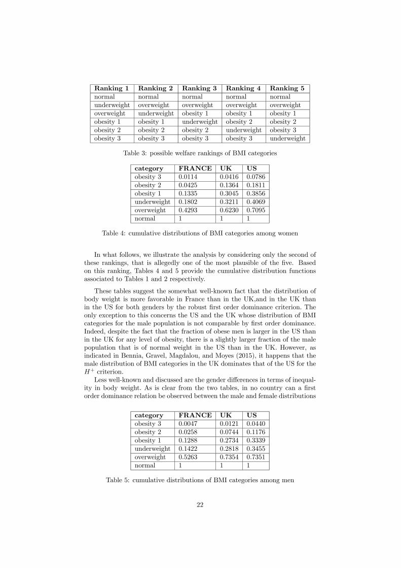
Ranking 1 Ranking 2 Ranking 3 Ranking 4 Ranking 5

normal normal normal normal normal

underweight overweight overweight overweight overweight

overweight underweight obesity 1 obesity 1 obesity 1

obesity 1 obesity 1 underweight obesity 2 obesity 2

obesity 2 obesity 2 obesity 2 underweight obesity 3

obesity 3 obesity 3 obesity 3 obesity 3 underweight

Table 3: possible welfare rankings of BMI categories

category FRANCE UK US

obesity 3 0.0114 0.0416 0.0786

obesity 2 0.0425 0.1364 0.1811

obesity 1 0.1335 0.3045 0.3856

underweight 0.1802 0.3211 0.4069

overweight 0.4293 0.6230 0.7095

normal 1 1 1

Table 4: cumulative distributions of BMI categories among women

In what follows, we illustrate the analysis by considering only the second of

these rankings, that is allegedly one of the most plausible of the five. Based

on this ranking, Tables 4 and 5 provide the cumulative distribution functions

associated to Tables 1 and 2 respectively.

These tables suggest the somewhat well-known fact that the distribution of

body weight is more favorable in France than in the UK,and in the UK than

in the US for both genders by the robust first order dominance criterion. The

only exception to this concerns the US and the UK whose distribution of BMI

categories for the male population is not comparable by first order dominance.

Indeed, despite the fact that the fraction of obese men is larger in the US than

in the UK for any level of obesity, there is a slightly larger fraction of the male

population that is of normal weight in the US than in the UK. However, as

indicated in Bennia, Gravel, Magdalou, and Moyes (2015), it happens that the

male distribution of BMI categories in the UK dominates that of the US for the

+ criterion.

Less well-known and discussed are the gender differences in terms of inequal-

ity in body weight. As is clear from the two tables, in no country can a first

order dominance relation be observed between the male and female distributions

category FRANCE UK US

obesity 3 0.0047 0.0121 0.0440

obesity 2 0.0258 0.0744 0.1176

obesity 1 0.1288 0.2734 0.3339

underweight 0.1422 0.2818 0.3455

overweight 0.5263 0.7354 0.7351

normal 1 1 1

Table 5: cumulative distributions of BMI categories among men

22

of BMI categories. Indeed, in all three countries, women are more affected by

obesity then men but women are also more likely to fall in the favorable "nor-

mal" weight category then men. However, it happens that the distribution of

BMI categories is "more equally" distributed among males than among females

as per the notion of equalization underlying Hammond transfers.

0

5

10

15

20

obesity 3 obesity 2 obesity 1 underweight overweight normal

Female H‐

Female H+

male H‐

male H+

Figure 2: H+ and H- curves for men and women en France, 2008.

For instance, Figure 2 shows the + and − curves for the female (in blue)and the male (in red) population in France. As can be seen, the males’ curves

lie everywhere below the females’ one. Hence, the distribution of BMI categories

appears to be more equally distributed among men than among women in France

for this ranking of BMI categories. As it happens, the same conclusion holds for

the two other countries. We believe that this male-female differential in body

weight inequalities revealed by our criteria is an important issue. It is also worth

mentioning that this conclusion of a better distribution of BMI categories among

men than among women could not be obtained using the well-known ordinal

criterion proposed by Allison and Foster (2004). In effect, the distributions of

BMI categories among males and among females do not have the same median.

As a result, Allison and Foster (2004) criterion does not even apply.

6 Conclusion

The paper has provided foundations to the issue of comparing alternative dis-

tributions of an attribute ordinally measured by an indicator that takes finitely

many values. The crux of the analysis has been an easy-to-use criterion, called

+−dominance, that can be viewed as the analogue, for comparing distribu-tions of an ordinally measurable attribute, of the generalized Lorenz curve used

for comparing distributions of a cardinally measurable one. It is well-known (see

23

e.g. Shorrocks (1983)) that a distribution of a cardinally measurable attribute

dominates another for the generalized Lorenz domination criterion if and only

if it is possible to go from the dominated distribution to the dominating one by

a finite sequence of increments of the attribute and/or Pigou-Dalton transfers.

The main result of this paper - Theorem 3 - establishes an analogous result

for the +-dominance criterion by showing that the latter criterion ranks two

distributions of an attribute in the same way than would the fact of going from

the dominated distribution to the dominating one by a finite sequence of incre-

ments and/or Hammond transfers of the attribute. The paper has also identified

a dual − dominance criterion that ranks two distributions in the same waythan would the fact of going from the dominated distribution to the dominat-

ing one by a finite sequence of decrements and/or Hammond transfers of the

attribute. We suspect strongly that the -dominance criterion - defined as the

intersection of the + and the − dominance one - coincides with the possibil-ity of going from the dominated distribution to the dominated one by a finite

sequence of Hammond transfers only.

As illustrated with the data provided in Bennia, Gravel, Magdalou, and

Moyes (2015), we believe the +-dominance criterion, and the Hammond prin-

ciple of transfers that justifies it along with increments, to be a useful tool for

comparing distributions of an attribute that can not be meaningfully transferred

à la Pigou-Dalton. Beside the fact of being justified by clear and meaningful

elementary transformations, the +-dominance criterion has the advantage of

being applicable to a much wider class of situations than, for instance, the widely

discussed criterion proposed by Allison and Foster (2004). The later is indeed

limited to distributions that have the same median. Furthermore it is not as-

sociated to clear and meaningful elementary transformations. The criterion

could also be useful for comparing distributions of a cardinally measurable at-

tribute if one is willing to accept the rather strong egalitarian ethics underlying

the principle of Hammond transfer.

Among the many possible extensions of the approach developped in this pa-

per, two strike us as particularly important. First, as the + criterion (or, for

that matter the one) is incomplete, it would be interesting to obtain simple

ordinal inequality indices that are compatible with Hammond transfers and,

therefore, with the criterion. We believe that obtaining an axiomatic charac-

terization of a family of such indices would not be too difficult. Indeed, a good

starting point would be to consider indices that can write as per expression (1)

for some suitable choice of lists (1 ) of real numbers. A second exten-

sion, that seems clearly more difficult, would be to consider multi-dimensional

attributes.

A Appendix: Proofs

A.1 Proposition 1

Let and 0 ∈ C be such that º1 0. By definition 5, one has (; ) ≤ (; 0)for all ∈ {1 }. It follows that:

(1; ) ≤ (1; 0)

24

and:

(1; ) + (2; ) ≤ (1; 0) + (2; 0),

2 (1; ) + (2; ) + (3; ) ≤ 2 (1; ) + (2; ) + (3; ),

−1X=1

¡2−−1

¢ (; ) + (; ) ≤

−1X=1

¡2−−1

¢ (; ) + (; ) ∀ = 2 3

as required by expressions (10) and (11) that define + dominance of 0 by . To

establish the − dominance of by 0, it suffices to notice that the requirement (; ) ≤ (; 0) for all ∈ {1 } that defines º1 0 can alternatively bewritten (thanks to expressions (17)-(19)) as :

(; ) ≥ ( 0)

for all ∈ {1 − 1}. This implies that: ( − 1; ) ≥ ( − 1; 0)

and:

( − 2; ) + ( − 1; ) ≥ ( − 2; 0) + ( − 1; 0), ( − 3; ) + ( − 2; ) + 2 ( − 1; ) ≥ ( − 3; 0) + ( − 2; 0) + 2 ( − 1; 0)

X=+1

¡2−−1

¢ (; )+ (; ) ≥

X=+1

¡2−−1

¢ (; 0)+ (; 0) ∀ = 1 2 −1

as required (thanks to expressions 22 and 23) by the − dominance of society bysociety 0 as per definition 7.

A.2 Lemma 1

Observe first that:

X=1

=

⎧⎪⎪⎨⎪⎪⎩1 1

+ 2 2+ · · ·+

(39)

or equivalently:

X=1

=

⎧⎪⎪⎪⎪⎨⎪⎪⎪⎪⎩1 1

+ 2 1 + 2 [2 − 1]

+ 3 1 + 3 [2 − 1] + 3 [3 − 2]

+ · · ·+ 1 + [2 − 1] + [3 − 2] + [ − −1]

(40)

hence:

X=1

=

⎧⎪⎪⎪⎪⎪⎨⎪⎪⎪⎪⎪⎩

1+ (− 1) [2 − 1]

+ [− (1 + 2)] [3 − 2]

+ · · ·+

h−P−1

=1

i[ − −1]

(41)

25

from which one obtains:

1

X=1

= [1 + ( − 1)]−−1X=1

(; )(+1 − ) (42)

= −−1X=1

(; )(+1 − ) (43)

as required by Equation (27). Now, by reconsidering equation (41) and recalling that

(; ) = 1 − (; ) =³−P

=1

´ for every = 1 , one immediately

obtains equation (28). We must now establish equation (29). For this sake, one can

notice that, for any ∈ {2 − 1}, one has:X

=1

=

X=1

+

X=+1

(44)

If one successively decompose the two terms on the right hand of (44), one obtains for

the first one:

X=1

=

⎧⎪⎪⎪⎪⎨⎪⎪⎪⎪⎩1 1

+ 2 1 + 2 [2 − 1]

+ 3 1 + 3 [2 − 1] + 3 [3 − 2]

+ · · ·+ 1 + [2 − 1] + [3 − 2] + [ − −1]

One has therefore:

X=1

=

⎧⎪⎪⎪⎪⎪⎪⎪⎪⎨⎪⎪⎪⎪⎪⎪⎪⎪⎩

³P=1

´1

+hP

=1 − 1

i[2 − 1]

+hP

=1 − (1 + 2)i[3 − 2]

+ · · ·+

hP=1 −

P−1=1

i[ − −1]

or equivalently:

1

X=1

=

Ã1

X=1

! −

−1X=1

(; ) [+1 − ] (45)

For the second term of (44), the successive decomposition yields:

X=+1

=

⎧⎪⎪⎪⎪⎨⎪⎪⎪⎪⎩+1 +1

+ +2 +1 + +2 [+2 − +1]

+ +3 +1 + +3 [+2 − +1] + +3 [+3 − +2]

+ · · ·+ +1 + [+2 − +1] + [+3 − +2] + [ − −1]

This can be written as:

X=+1

=

⎧⎪⎪⎪⎪⎪⎪⎪⎨⎪⎪⎪⎪⎪⎪⎪⎩

³P=+1

´+1

+³P

=+2

´[+2 − +1]

+³P

=+3

´[+3 − +2]

+ · · ·+ [ − −1]

26

or equivalently:

1

X=+1

=

Ã1

X=+1

!+1 +

−1X=+1

(; ) [+1 − ] (46)

By summing equations (45) and (46), one concludes that:

1

X=1

=

Ã1

X=1

! +

Ã1

X=+1

!+1

−−1X=1

(; ) [+1 − ] +

−1X=+1

(; ) [+1 − ](47)

This equality can be further simplified, by observing that:Ã1

X=1

! +

Ã1

X=+1

!+1 =

1

Ã−

X=+1

! +

Ã1

X=+1

!+1

= + (+1 − ) (; ) (48)

Equation (29) is then obtained from the reintroduction of (48) into (47).

A.3 Propositions 2 and 3

For proposition 2, let be a society obtained from 0 by an increment. By definition2, there exists some ∈ {1 − 1} such that:

= 0

for all ∈ {1 } such that 6= + 1,

= 0 − 1

and,

+1 = 0 + 1.

Then ºA 0 if and only if: (using definition 1):

X=1

≥X

=1

0

⇐⇒+1 − ≥ 0

by definition of an increment. As this inequality must hold for any ∈ {1 − 1},this completes the proof of proposition 2.The argument for the proof of proposition 3

is similar (with definition 2 replaced by definition 3.

27

A.4 Theorem 1

The equivalence between statements (a) and (c) of this theorem is well-known in the

literature. We therefore only prove the equivalence between statements (b) and (c).

Using equation (27) of Lemma 1, one has:

1

"X

=1

−X

=1

0

#=

−1X=1

[ (; 0)− (; )] [+1 − ] (49)

Hence, if º1 0 and (1 ) ∈ A+1 , thenP

=1 ≥P

=1 0 . To

establish the converse implication, define, for every ∈ {1 − 1} the list of numbers = (1

) to be such that

= 0 for = 1 and

= 1 for

= + 1 . We note that ∈ A+1 for any ∈ {1 − 1}. Since ºA+10,

one must therefore have, for any = 1 − 1:X

=1

≥

X=1

0

⇐⇒X

=+1

≥X

=+1

0

⇐⇒

−X

=1

≥ −X

=1

0

⇐⇒X

=1

≤X

=1

0

as required (definition 5) for º1 0.

A.5 Proposition 4

Suppose that society has been obtained from society 0 by means of a Hammondtransfer as per Definition 4. This means that there are categories 1 ≤ ≤

≤ for which one has:

X=1

=

X=1

0 − + + − (50)

By definition 1, ºA 0 for any obtained from 0 by means of a Hammond transferif and only if inequality

P=1

−

P=1

0 = ( − ) − ( − ) ≥ 0

hold for all categories 1 ≤ ≤ ≤ , which is precisely the definition of the

setAH.

28

A.6 Proposition 5

Assume that the list of numbers (1 ) belongs toAH and, therefore, satisfies

− ≥ − for all 1 ≤ ≤ ≤ . This implies in particular

that +1 − ≥ − +1 for any ∈ {1 2 − 2}. Let = min{ =1 : +1 − ≤ 0} (using the convention that +1 = ). Such a clearly

exists under this convention, because ∈ { = 1 : +1 − ≤ 0}. If = ,

then the fact that +1 − ≥ − +1 holds for any ∈ {1 2 − 2}implies that +1 − ≥ − +1 for all = 1 2 − 1 and (trivially) that0+1−0 ≤ 0− holds for all 0 ∈ { −1} = ∅. Notice that if = , then,

one has +1 − ≥ − +1 0 for any ∈ {1 2 − 2} (the alphas are

increasing with respect to the categories). If = 1, then the set { = 1 2 −1} isempty so that one must simply verify that 0+1−0 ≤ 0−1, for 0 = 1 −1.But this results immediately from the definition of (if 0 = 1) or from applying the

requirement that − ≥ − for all 1 ≤ ≤ ≤ to the

particular case where = 1, = = 0 1 and = 0 + 1 (otherwise). Noticethat if = 1, then one has by definition that 0 ≥ 2 − 1 ≥ − −1 forevery = 3 so that the alphas are decreasing with the categories. Assume now

that ∈ {2 − 1}. We must check first that +1 − ≥ − +1 for all

= 1 2 −1. The case where = −1 is proved by observing that, by definitionof , one has − −1 0 = − . The case where − 1 (if any) is provedby applying the statement − ≥ − for all 1 ≤ ≤ ≤ to the

particular case where = ∈ {1 −2} = = +1 and = . To check that the

inequality 0+1−0 ≤ 0− holds for all 0 ∈ {0 −1}, simply observe that,for 0 = , the inequality is obtained from the very definition of and, for 0 , it

results from applying the fact that − ≥ − for all 1 ≤ ≤ ≤

to the particular case where = , = = 0 and = 0 + 1Conversely, consider any list of numbers (1 ) for which there exists a ∈{1 } such that:

+1 − ≥ − +1 (51)

holds for all ∈ {1 2 − 1} (if any) and:0+1 − 0 ≤ 0 − (52)

holds for all 0 ∈ { −1} (if any). Notice that applying inequality (51) to = −1implies that − −1 ≥ − = 0. Combining this recursively with inequality

(51) implies in turns that 2 − 1 ≥ 3 − 2 ≥ ≥ − −1 ≥ 0 so that thelist of numbers (1 ) is increasing from 1 up to . Similarly, applying inequality

(52) to 0 = implies that +1 − ≤ − = 0. Combining this recursively

with inequality (52) satisfied for all 0 ∈ { − 1} (if any) leads to the conclusionthat − −1 ≤ −1 − −2 ≤ ≤ +1 − ≤ 0 so that the list of numbers(1 ) is decreasing from up to . Consider then any four integers , , and

satisfying 1 ≤ ≤ ≤ . Five cases need to be distinguished:

(i) ≥ ≥ 1, then one has: − = ( − −1) + (−1 − −2) + + (+1 − )

≤ +1 − (because the are decreasing above )

≤ − (by inequality (52))

= − + − + − (for any integer )

≤ − (because the are decreasing above )

29

(ii) ≤ ≤ ≤ . Then one has:

− = ( − −1) + (−1 − −2) + + (+1 − )

≤ +1 − (because the are decreasing above )

≤ − (by inequality (52))

= − + − + − (for any integer )

≤ − (because − ≤ 0 and − ≤ 0)

(iii) ≤ ≤ . Then one has:

− = ( − −1) + (−1 − −2) + + (+1 − )

≤ +1 − (because the are decreasing above )

≤ − (by inequality (52))

≤ 0 (because the are decreasing above )

≤ − (because the are increasing below )

(iv) ≤ ≤ ≤ . Then one has:

− = ( − −1) + (−1 − −2) + + (+2 − +1) + (+1 − )

≥ +1 − (because the are increasing below )

≥ − +1 (by inequality (51))

= − + − + − +1 (for any + 1 ≤ ≤ )

≥ − (because − ≥ 0 and − +1 ≥ 0)

(v) ≤ . In this case, one has:

− = ( − −1) + (−1 − −2) + + (+2 − +1) + (+1 − )

≥ +1 − (because the are increasing below )

≥ − +1 (by inequality (51))

= − + − + − +1 (for any + 1 ≤ ≤ )

≥ − (because because the are increasing below )

Hence any list of numbers (1 ) for which there exists a ∈ {1 } suchthat inequalities (52) and (51) belongs to AH.

A.7 Theorem 3.

A.7.1 Statement (a) implies statement (b)

Suppose has been obtained from 0 by means of an increment. It then follows fromProposition 2 that inequality 1 holds for all ordered lists of real numbers (1 )

in the set A+1 . This inequality holds therefore in particular for all ordered lists of

real numbers (1 ) in the set A+H ⊂ A+1 . If, on the other hand, has beenobtained from 0 by means of a Hammond transfer, we know from Proposition 4 that

inequality 1 holds for all ordered lists of real numbers (1 ) in the set AHand, therefore, for all ordered list of real numbers in the set A+H ⊂ AH. Sincethe binary relation ºA+

His transitive, the implication then follows from any finite

repetition of these two elementary implications.

30

A.7.2 Statement (b) implies statement (c)

Assume thatX=1

≥X=1

0 (53)

holds for all (1 ) ∈ A+H. For any ∈ {1 }, define the ordered list of numbers (1

) by:

= −(2−) for = 1 = 0 for = + 1

Let us first show that the ordered list (1 ) of real numbers thus defined

belongs to A+H for every ∈ {1 }. Thanks to Lemma 2, this amounts to showthat these real numbers satisfy

+1 − ≥ − +1 (54)

for every ∈ {1 − 1}. If ≥ + 1, then one has:

+1 − = 0− 0 ≥ 0− 0 = − +1

so that that inequality (54) holds for that case. If = , then

+1 − = 0 + 20 ≥ 0− 0 = − +1

so that (54) holds also for that case. If finally , then one has:

+1 − = −2−−1 + 2−= 2−−1

= 0− (−2−−1)= − +1

so that inequality (54) holds for this case as well. Since the ordered list (1 )

of real numbers belongs to A+H for every ∈ {1 }, Inequality (53) must hold forany such ordered list of numbers. Hence, one has, for every ∈ {1 } :

X=1

≥

X=1

0

⇐⇒X

=1

2− ≤X

=1

2−0

which is nothing else than the condition for + dominance, as expressed by equation

(9).

A.7.3 Statement (c) implies statement (a)

Assume that º+ 0 so that +(; ) ≤ +(; 0) for all = 1 2 − 1.We know from Proposition 1 that º1 0 implies º+ 0. Hence, if º1 0, weconclude from theorem 1 that can be obtained from 0 by means of a finite sequence of

31

increments and the proof is done. In the following, we therefore assume that º+ 0

holds but that º1 0 does not hold so that there exists some ∈ {1 2 − 1}for which one has (; )− (; 0) 0. Define then the index by:

= min { | (; )− (; 0) 0} (55)

Given that index , one can also define the index by:

= min { | (; )− (; 0) ≤ 0 ∀ ∈ [ ]} (56)

Such a exists because (; )− (; 0) = 0. Notice that, by definition of such a ,one has:

( − 1; )− ( − 1; 0) 0 and (; )− (; 0) ≤ 0 (57)

Hence, one has (using the definition of provided by (7), that 0 . We now

establish that there exists some ∈ {1 2 − 1} such that: (; )− (; 0) 0 and (; )− ( 0) = 0 ∀ (58)

Indeed, since +(; ) ≤ +(; 0) for all = 1 2 − 1, one has either:+(1; ) +(1; 0)

⇐⇒ (thanks to expression (10))

(1; ) (1; 0) (59)

or:

(1; ) = (1; 0) (60)

If case (59) holds, then the existence of some ∈ {1 2 −1} for which expression(58) holds is established (with = 1). If, on the other hand, case (60) holds, then,

since +(2; ) ≤ +(2; 0) holds, we must have either:

+(2; ) +(2; 0)

⇐⇒ (thanks to expression (11))

2 (1; ) + (2; ) 2 (1; 0) + (2; 0) (61)

or:

2 (1; ) + (2; ) = 2 (1; 0) + (2; 0) (62)

Again, if we are in case (61), we can conclude (since (1; ) = (1; 0)) that (2; ) (2; 0), which establishes the existence of some ∈ {1 2 − 1} for whichexpression (58) holds (with = 2 in that case). If we are in case (62), we iterate in the

same fashion using the definition of + provided by (11). We notice that the index

for which (58) holds must be strictly smaller than because assuming otherwise will

contradict, given the definition of and the (iterated as above) definition of +, the

fact that +(; ) ≤ +(; 0) holds for all = 1 2 − 1. We finally notethat, because of the definition of provided by (7), the definition of the index just

provided entails that:

0 (63)

and:

= 0

32

for all = 1 − 1. We now proceed by defining a new society - 1 say - that

belongs to C, that has been obtained from 0 by means of a Hammond’s transfersand that is such that º+ 1 Â+ 0. For this sake, we define the numbers 1 and2 and by:

1 = 0 − ; 2 = [ ( − 1; )− ( − 1; 0)] and = min(1 2) (64)

We note that, by the very definition of the index , one has 1 0. We notice also

that, using (57) and the definition of the index , one has 0 2 ≤ 0 − . Define

then the society 1 by:

1

= 0 ∀ 6= + 1 ;

1

= 0 − ;

1

+1 = 0+1 + 2 ;

1

= 0 − ;

It is clear that such a society belongs to C. Moreover, 1 has been obtained from0 by Hammond transfers as per definition 4 where the indices and of this

definition are, here, , + 1, + 1 and (respectively)). By virtue of what has been

established above, this implies that 1 Â+ 0. We further notice that:

( 1) =

X=1

1

=

X=1

0

= ( 0) (66)

for all = 1 − 1. Also one has:

( 1) =

X=1

1

= (− 1 0) + 1

= (− 1 0) + (0 − )

= ( 0)− (67)

(+ 1 1) = ( 1) + 1

+1

= ( 0)− + 1

+1

= ( 0)− + 0+1+ 2

= (+ 1 0) + (68)

Furthermore, for = + 2 − 1, one has:

( 1) = (+ 1 1) +

X=+2

1

= (+ 1 0) + +

X=+2

1

= (+ 1 0) + +

X=+2

0

= ( 0) + (69)

33

While finally, for = :

( 1) = ( − 1 1) +X=

1

= ( − 1 0) + +

X=

1

= ( − 1 0) + + 0 − +

X=+1

0

= ( 0) (70)

We must now verify that º+ 1 and, therefore, that +(; )−+(; 1) ≤ 0 forall = 1 2 −1. Since º+ 0, we know already that +(; )−+( 0) ≤0 for all = 1 2 − 1. We first observe that, by the definition just given of 1one has:

+( 1) =

⎧⎪⎪⎨⎪⎪⎩+( 0) for = 1 − 1,+( 0)− for = ,

+( 0) for = + 1 − 1+( 0)− 2− for = .

(71)

The first line of (71) is indeed clear given expression (66) and the definition of +

provided by (9).The second line of (71) results from (67) and the definition of +

provided by (11). Consider now = + 1. One has (using (11) again):

+(+ 1 1) =

X=1

¡2−

¢ (; 1) + (+ 1; 1)

=

−1X=1

¡2−

¢ (; 0) + (; 0)− + (+ 1; 1) (by (67))

=

−1X=1

¡2−

¢ (; 0) + (; 0)− + (+ 1; 0) + (by (68))

=

−1X=1

¡2−

¢ (; 0) + (; 0) + (+ 1; 0)

=

X=1

¡2−

¢ (; 0) + (+ 1; 0) = +(+ 1 0) (72)

Combined with (12) and the fact that 1

= 0 for all = + 2 − 1, equality

(72) establishes the third line of expression (71). As for the last line of (71), we start

with = and we use (12) to write:

+( 1) = 2+( − 1; 1) + 1

= 2+( − 1; 0) + (0 − )

= +( 0)− (73)

34

Iterating on this expression using (12) yields:

+( + 1 1) = 2+(; 1) + 1

+1

= 2(+(; 0)− ) + 0+1

= +( + 1 0)− 2 (74)

and therefore, for any ∈ { }:

+( 1) = +( 0)− 2−

as required by the last line of expression (71). We now notice that expression (71)

entails that:

+( )−+( 1) =

⎧⎪⎪⎨⎪⎪⎩+( )−+( 0) for = 1 − 1,+( )−+( 0) + for = ,

+( )−+( 0) for = + 1 − 1+( )−+( 0) + 2− for = .

(75)

Since by assumption º+ 0, this establishes that +(; ) −+(; 1) ≤ 0 forall ∈ {1 2 − 1}∪ {+1 − 1}. Consider now the case = . Using (12),

we know that:

+(; )−+( 0) = 2 (+(− 1; )−+(− 1; 0)) + ( − 0 ) (76)

By definition of , one has (; ) − (; 0) = 0 for all , so that the first

term in the right hand side of equation (76) is 0. Recalling then from (64) that

1 = 0 − 0 and that = min(1 2), it follows that:

− 0 + ≤ 0

By combining equations (75) and (76), we conclude that:

+( )−+( 1) = +( )−+( 0) + = − 0 + ≤ 0 (77)

Consider finally the case where = −1. By using equation (12) (and recallingthat 2 = [ ( − 1; )− ( − 1; 0)]), one has:

+(; )−+(; 0) = 2(+(− 1; )−+(− 1; 0))+ (; )− (; 0)− 2

(78)

Combining (78) with the last line of (75), and remembering that ≤ 2, one obtains:

+( )−+( 1) = 2[(+(−1; )−+(−1; 0)]+ (; )− (; 0)+(−2) ≤ 0 (79)

Finally, using successive applications of equation (12), one obtains, for any = +

1 − 1:

+(; )−+(; 0) = 2−+1[+( − 1; )−+( − 1; 0)]

+

−1X=

2−1−[ (; )− (; 0)]

+ (; )− (; 0)− 2−2≤ 0

35

by assumption. Combined with the last line of (75) and the fact that ≤ 2, this

completes the proof that º+ 1. Hence, we have found a society 1 obtained from

society 0 by means of a Hammond’s transfers that is such that º+ 1 Â+ 0.We now show that, in moving from 0 to , one has "brought to naught" at least oneof the differences | (; )− (; 0)| that distinguishes from 0. That is to say, weestablish the existence of some ∈ {1 − 1} for which one has:¯

(; )− (; 1)¯= 0

and:

| (; )− (; 0)| 0This is easily seen from the fact that, in the construction of 1, one has either:

= 1 = 0 − (80)

or:

= 2 = [ ( − 1; )− ( − 1; 0)] (81)

If we are in the case (80), one has by definition of the index and the function :

(; )− (; 1) = 0

and:

(; )− (; 0) 0

If on the other hand we are in case (81), then, we have (using (68)):

( − 1; )− ( − 1; 1) = ( − 1 )− [ ( − 1 0) + 2]

= 0

while, by definition of the index , one has:

( − 1 )− ( − 1 0) 0

Now, if = 1, then the proof is complete. If ¬( = 1) but º1 1, then we

conclude that society can be obtained from society 0 by means of a finite sequenceof Hammond’s transfers and increments. If ¬( = 1) and ¬© º1 1ª, then wecan find three categories and just as in the preceding step and construct a new

distribution - say 2 - that can be obtained from distribution 1 by means of an

(integer number of) Hammond’ transfers satisfying º+ 2 Â+ 1 and so on.

More generally, after a finite number - say - of iterations, we will find a distribution

such that º+ Â+ −1 . In that case, we will have either = or º1 .As is finite, and there are finitely many differences of the kind | (; )− (; 0)|to bring to naught, this completes the proof.

A.8 Theorem 4

A.8.1 Statement (a) implies statement (b)

Just like the (detailed) argument underlying the proof of the corresponding implication

for Theorem 3, the implication results straightforwardly from Propositions 3 and 4.

36

A.8.2 Statement (b) implies statement (c)

Assume that the inequality:

X=1

≥X=1

0 (82)

holds for all (1 ) ∈ A−H . For any = 1 − 1, define the ordered list of numbers (1

) by:

= 0 for = 1

= −2−−1 for = + 1 (83)

We first show that, for any ∈ {1 −1}, (1 ) ∈ A−H. Thanks to Lemma3, this amounts to show that, for any ∈ {1 − 1}, one has:

+1 − ≤ − 1 ≤ 0 (84)

for all ∈ {1 − 1}. If ≤ − 1, then one has (thanks to expression (83)):

+1 − = 0− 0 ≤ − 1 = 0− 0 = 0

so that (84) holds for those . If = , then one has (expression (83)):

+1 − = +1 − = −1 ≤ − 1 = 0− 0 = 0

so that (84) holds for that case. Assume now that ≥ + 1. In that case, one has

by expression (83):

+1 − = −2− + 2−−1= −2−−1= − 1 ≤ 0

so that (84) holds for those as well. Since the ordered lists of numbers (1 )

defined by (83) all belong to A−H, inequality (82) holds for any of those ordered lists.As a result, one has:

X=1

≥

X=1

0

⇐⇒X

=+1

2−−1 ≤

X=+1

0 2

−−1

for every = 1 −1, which, by expression (20), is the definition of − dominance.

A.8.3 Statement (c) implies statement (a)

Assume that º− 0, so that −(; ) ≤ −(; 0) for all = 1 2 − 1(avoiding the degenerate case where is equal to 0).Step 1.

37

From Proposition 1, 0 º1 implies º− 0. By Theorem 1, 0 º1 if and

only if 0 can be obtained from by a finite sequence of increments or, equivalently,

if can be obtained from 0 by a finite sequence of decrements. Hence, if 0 º1 ,

we know that can be obtained from 0 by means of a finite sequence of decrements,and the proof is complete. In the following, we therefore assume that º− 0

but that 0 º1 does not hold. Hence, there exists ∈ {1 2 − 1} such that (; 0)− (; ) 0, or, equivalently, such that:

1− (; ) 1− (; 0)

⇐⇒ (; ) (; 0)

Let be defined by:

= max© | (; )− (; 0) 0

ª (85)

Given , we let be defined by:

= max© | (− 1; )− (− 1; 0) ≤ 0ª (86)

Such a exists because (0; )− (0; 0) = 0. By definition, we have:

( − 1; )− ( − 1; 0) ≤ 0 and (; )− (; 0) 0 (87)

from which we deduce that 0 .We now prove the existence of some ∈ { + 2 } such that:

(− 1; )− (− 1; 0) 0 and (; )− (; 0) = 0 ∀ − 1 (88)

Note that if such a exists, equation (88) implies that 0. To prove theexistence of a such that (88) holds, one first recall that º− 0 if and only if−(; ) −−(; 0) ≤ 0 for all = 1 2 − 1. If −( − 1; ) −−( −1; 0) 0 or, equivalently, if ( − 1; ) − ( − 1; 0) 0, one has =

and 0 . If, otherwise, −( − 1; ) − −( − 1; 0) = 0 or, equivalently,

(−1; )− (−1; 0) = 0, one can move forward and recall that −(−2; )−−( − 2; 0) ≤ 0. If −( − 2; ) −−( − 2; 0) 0, one obtains, using (??),

that [ (− 1; )− (− 1; 0)] + [ (− 2; )− (− 2; 0)] 0. When combinedwith (− 1; )− (− 1; 0) = 0, this implies that (− 2; )− (− 2; 0) 0so that one can set = − 1, and observe that 0 and −1 0−1. Ifon the other hand −( − 2; )−−(2; 0) = 0, then one can proceed to the nextiteration (and so on until one gets eventually to + 2). It can not be the case that

(+; )− (+; 0) = 0 for all = 1 − − 1 because assuming so wouldamount, when combined with the definition of provided by (85) and the definition

of −() provided by (23), to contradicting the fact that −(; )−−(; 0) ≤ 0for all = 1 2 − 1.Step 2.

We now define a new society 1 ∈ C, obtained from 0 by means of a finitesequence of Hammond transfers, and such that º− 1. We start by setting:

1 = ×£ (; )− (; 0)¤; 2 = ×£ (− 1; 0)− (− 1; )¤ and = min {1 ; 2}

(89)

38

From equation (88), we have 2 = 0− 0. Then, it is apparent from (87) that

0 1 ≤ 0 − . Moreover, since and 0 ∈ N+ for all = 1 2 , one

also has 1 2 ∈ N+, which implies that ∈ N+. We then define the society 1 asfollows:

1

= 0 ∀ 6= − 1 ;

1

= 0 − ; 1

−1 = 0−1 + 2 ; 1

= 0 −

By construction, 1 ∈ , and 1 is obtained from by means of exactly ∈ N++Hammond’s transfers. Observe now that:

−(; )−−(; 1) =

⎧⎪⎪⎨⎪⎪⎩−(; )−−(; 0) +

¡2−−1

¢ for = 1 − 1

−(; )−−(; 0) for = − 2−(; )−−(; 0) + for = − 1−(; )−−(; 0) for = − 1

(92)

Since º− 0 or, equivalently, −(; )−−(; 0) ≤ 0 for all = 1 2 −1, if follows from (92) that −(; ) − −(; 1) ≤ 0 for all ∈ { −2}S{ − 1}. Consider now the case where = − 1. Using (??), one has:

−(−1; )−−(−1; 0) = 2 £−(; )−−(; 0)¤+1

(−0) (93)

Remember that (; ) − (; 0) = 0 by definition of . Remember also that

2 = 0 − 0 and that = min {1 ; 2} so that ≤ (0 − ). Hence,

combining equations (92) and (93) leads to the conclusion that:

−(− 1; )−−(− 1; 1) =

− 1

(0 − ) ≤ 0 (94)

Consider finally the cases where = 1 −1 Start with the case where = −1.By using equation (??), and recalling that 1 = × £ (; )− (; 0)

¤, one observes

that:

−(−1; )−−(−1; 0) = 2 £−(; )−−(; 0)¤+ (−1; )− (−1; 0)−1

(95)

Combining (95) with (92) yields:

−(−1; )−−(−1; 1) = 2 £−(; )−−(; 0)¤+ (−1; )− (−1; 0)+ − 1

≤ 0

(96)

(since −(; )−−(; 0) ≤ 0 and (−1) ≤ 0). Finally, by successive applicationsof equation (??), one obtains, for any = 1 − 2:−(; )−−(; 0) = (2−)

£−(; )−−(; 0)

¤+ ( − 1; )− ( − 1; 0)

−(2−−1)1+

−1X=+1

(2−−1)[ (; )− (; 0)] (97)

Combining (97) with (92) one obtains, for all = 1 − 2:−(; )−−(; 1) = (2−)

£−(; )−−(; 0)

¤+ ( − 1; )− ( − 1; 0)

+(2−−1) − 1

+

−1X=+1

(2−−1)[ (; )− (; 0)]

≤ 0

39

(since −(; ) − −(; 0) ≤ 0, − 1 and (; ) − (; 0) ≤ 0 for all =

1 − 1). Hence, −(; ) ≤ −(; 1) for all = 1 − 1 and, therefore, º− 1.

Step 3.Hence, we have found a society 1 obtained from society 0 by means of a sequence

of Hammond’s transfers that is such that º− 1 Â− 0. We now show that, inmoving from 0 to 1, one has "brought to naught" at least one of the differences¯ (; )− (; 0)

¯that distinguishes from 0. That is, we establish the existence

of some ∈ {1 − 1} for which one has:¯ (; )− (; 1)

¯= 0

and:

| (; )− (; 0)| 0This is easily seen from the fact that, in the construction of 1, one has either:

= 1 = × £ (; )− (; 0)¤

(98)

or:

= 2 = 0 − (99)

If we are in the case (99), one has by definition of the index and the function :

(− 1; )− (− 1; 1) = 0

and:

(− 1; )− (− 1; 0) 0

=⇒| (− 1; )− (− 1; 0)| 0

If, on the other hand, we are in case (98), then, we have (using (68)):

(; )− (; 1) = ( )− [ ( 0) + 2]

= 0

while, by definition of the index , one has:

( )− ( 0) 0

Now, if = 1, then the proof is complete. If 6= 1 and 1 º1 , then we

conclude that society can be obtained from society 0 by means of a finite sequenceof Hammond’s transfers and decrements. If 6= 1 and ¬(1 º1 ), then we can

find three categories and just as in the preceding step and construct a new

distribution - say 2 - that can be obtained from distribution 1 by means of an

(integer number of) Hammond’ transfers satisfying º− 2 Â− 1 and so on.

More generally, after a finite number - say - of iterations, we will find a distribution

such that º− Â− −1 . In that case, one has either = or º1 .As is finite, and there are finitely many differences of the kind

¯ (; )− (; 0)

¯to bring to naught, this completes the proof.

40

A.9 Theorem 5

A.9.1 Statement (a) implies statement (b)

This results immediately from the definition of the set AH (using Proposition 4).

A.9.2 Statement (b) implies statement (c)

Assume that the inequalityP

=1 ≥

P=1

0 holds for all lists of real

numbers (1 ) ∈ A . This implies in particular that the inequality holds for

all (1 ) ∈ A+ so that ºA+H0 holds. It then follows from Theorem 3 that

º+ 0. Similarly, the fact that the inequalityP

=1 ≥

P=1

0 holds

for all lists of real numbers (1 ) ∈ A implies in particular that it holds for

all (1 ) ∈ A− . Hence ºA−H 0 holds and, thanks to Theorem 4, so does

º− 0. Hence one has both º+ 0 and º− 0, as required by the definitionof º

A.9.3 Statement (c) implies statement (b)

Assume that º 0. Thanks to Proposition 5, one needs to show thatP

=1 ≥P

=1 0 holds for all (1 ) ∈ R+ for which there exists an integer ∈

{1 } such that (+1−) ≥ (−+1), for all = 1 2 −1 (if any) and(0+1 − 0) ≤ (0 − 0), for all ∈ { + 1 − 1} (again if this set is non-empty). Since by definition of º , one has both º+ 0 and º− 0, we knowat once from Theorems 3 and 4 that

P=1

≥

P=1

0 holds for all list of

real numbers (1 ) ∈ A+ ∩ A− . These numbers are associated to an integer ∈ {1 }. Hence one only needs to prove that P

=1 ≥

P=1

0 holds for

all (1 ) ∈ R+ for which there exists an integer ∈ {2 − 1} such that(+1−) ≥ (−+1), for all = 1 2 −1 and (0+1−0) ≤ (0 −0)for all = { + 1 − 1}. Using (28) in Lemma 1, we find useful to write (forany society ):

1

X=1

= −−1X=1

(; ) [+1 − ] (100)

or:

1

X=1

= −−1X=1

( ) (101)

with = +1 − for every = 1 − 1. Letting = −P−1

=+1 for

all = 1 2 − 2 a[nd −1 = −1, we rewriteP−1

=1 ( ) in (101) as

follows:

For = 1:

41

(1; )1 = (1; )[1 −−1X=2

] + (1; )2++ (1; )−1

= (1; )[1 −−1X=2

] + (1; )[2 −−1X=3

]

+2 (1; )3 ++ 2 (1; )−1

= (1; )[1 −−1X=2

] + (1; )[2 −−1X=3

]

+2 (1; )[3 −−1X=4

] +4 (1; )4+ 4 (1; )−1

=

= (1; )1+ (1; )2+2 (1; )2 (102)

+ 22 (1; )3++ 2−3 (1; )−1

For = 2

(2; )2 = (2; )[2 −−1X=3

]+ (2; )3++ (2; )−1

= (2; )[2 −−1X=3

]+ (2; )[3 −−1X=4

]

+2 (2; )4++ 2 (2; )−1

= (2; )[2 −−1X=3

] + (2; )[3 −−1X=3

]

+2 (2; )[4 −−1X=5

] + 4 (2; )5+ 4 (2; )−1

=

= (2; )2+ (2; )3+2 (2; )4 (103)

+22 (2; )5++ 2−4 (2; )−1

More generally, one has ( − 1 )−1 = ( − 1; )−1 and, for all =

1 2 − 2:

(; ) = (; ) + (; )

−1X=+1

¡2−−1

¢ (104)

42

Hence, one can write:

(1;)1 = (1;)1 + (1;)2 + 2 (1;)3 + 22 (1;)4 + + 2−4 (1;)−2 + 2−3 (1;)−1 (2;)2 = (2;)2 + (2;)3 + 2 (2;)4 + 2−5 (2;)−2 + 2−4 (2;)−1 (3;)3 = (3;)3 + (3;)4 + 2−6 (3;)−2 + 2−5 (3;)−1 (4;)4 = (4;)4 + 2−7 (4;)−2 + 2−6 (4;)−1

(−2;)−2 = + (−2;)−2 + (−2;)−1 (−1;)−1 = + (−1;)−1

(105)Remembering that −1 = −1 and = −

P−1=+1 for all = 1 2 −2,

one can use equation (11) and sum vertically the decomposition (105) to obtain:

−1X=1

(; ) =

−1X=1

+(; )[ −−1X

=+1

] (106)

Since 1

P=1

= −

P−1=1 (; ) , one obtains finally:

1

[

X=1

−X=1

0 ] =−1X=1

£+(; 0)−+(; )

¤[ −

−1X=+1

] (107)

In a symmetric fashion, one obtains from equation (28) in Lemma 1:

1

X=1

= 1 +

−1X=1

(; ) [+1 − ] (108)

Hence, letting 1 = 1 and = (−P−1

=1 ) for all = 2 3 −1, we rewriteP−1=1 (; ) [+1 − ] in (108) as follows:

For = − 1:

( − 1; )−1 = ( − 1; )[−1 −−2X=1

] + ( − 1; )−2 + + ( − 1; )1

= ( − 1; )[−1 −−2X=1

] + ( − 1; )[−2 −−3X=1

]

+2 ( − 1; )−3 + + 2 ( − 1; )1

= ( − 1; )[−1 −−2X=1

] + ( − 1; )[−2 −−3X=1

]

+2 ( − 1; )[−3 −−4X=1

] + 4 ( − 1; )−4+ 4 ( − 1; )1=

= ( − 1; )−1 + ( − 1; )−2 + 2 ( − 1; )−3 (109)

+22 ( − 1; )−4 + + 2−32 ( − 1; )1For = − 2:

43

( − 2; )−2 = ( − 2; )[−2 −−3X=1

] + ( − 2; )−3

+ ( − 2; )−4 + + ( − 2; )1

= ( − 2; )[−2 −−3X=1

] + ( − 2; )[−3 −−4X=1

]

+2 ( − 2; )−4 + + 2 ( − 2; )1

= ( − 2; )[−2 −−3X=1

] + ( − 2; )[−3 −−4X=1

]

+2 ( − 2; )[−4 −−5X=1

]

+4 ( − 2; )−5 ++ 4 ( − 2; )1=

= ( − 2; )−2 + ( − 2; )−3 + 2 ( − 2; )−4(110)

+22 ( − 2; )−5 + + 2−42 ( − 2; )1More generally, one has (1; )1 = (1; )1 and:

(; ) = (; ) + (; )

−1X=1

¡2−−1

¢ ∀ = 2 3 − 1 (111)

Hence, one can conclude that:

( − 1; )−1 = ( − 1; )−1 + ( − 1; )−2 + + 2−4 ( − 1; )2 + 2−3 ( − 1; )1 ( − 2; )−2 = ( − 2; )−2 + · · ·+ 2−5 ( − 2; )2 + 2−4 ( − 2; )1

=

(2; )2 = (2; )2 + (2; )1

(1; )1 = + (1; )1(112)

Using (23), and summing vertically the previous equation, one obtains:

−1X=1

(; ) = −(1; )1 +−1X=2

−(1; )[ −−1X=1

] (113)

These decompositions being obtained, consider now an integer ∈ {2 3 − 1}such that:

−1 ≥ 0 and ( −−1X

=+1

) ≥ 0 for = 1 − 2 (114)

and:

≤ 0 and ( −−1X=

) ≤ 0 for = + 1 − 1 (115)

44

From Equation (29) in Lemma 1, one has, for any such a ∈ {2 3 − 1}:

1

X=1

= −−1X=1

(; ) +

−1X=

(; ) (116)

By using equations (102) - (107) and replacing category by category in these

equations, one obtains:

−1X=1

(; ) =

−2X=1

+(; )

" −

−1X=+1

#++(− 1; ) −1 (117)

Symmetrically, replacing category 1 by category in equations (108)-(113) enables one

to write:

−1X=

(; ) = −(; ) +−1X=+1

−(; )

" −

−1X=

# (118)

Combining equations (116), (117) and (118), one gets finally:

1

[

X=1

( − 0 )] =

−2X=1

[+(; 0)−+(; )]

" −

−1X=+1

#+[+(− 1; 0)−+(− 1; )] −1+[−(; )−−(; 0)]

+

−1X=+1

[−(; )−−(; 0)]

" −

−1X=

#(119)

Since º 0, one has both º+ 0 and º− 0. Hence+(; )−+(; 0) ≤ 0and −(; )−−(; ) ≤ 0 for all ∈ C. This, combined with equations (114) and(114), leads to the conclusion that each term of the right hand side of Equality (119)

is positive, and, therefore, that

X=1

( − 0 ) ≥ 0 for all lists of real numbers

(1 ) in the set A , as required by normative dominance.

A.10 Proposition 6

Assume that º+ 0 and, thanks to Theorem 3, that can be obtained from 0 bymeans of a finite sequence of increments and/or Hammond transfers. We immediately

deduce from this information that the smallest ∈ {1 2 } for which 6= 0is such that 0 . But this implies that º 0. To show that the converse

implication is false, one just needs to consider the following example for = = 3,

and societies and 0 such that:

01 = 1 02 = 0,

03 = 2

and:

1 = 3 = 0, 2 = 3

45

It is clear that º 0. The conclusion that º+ 0 does not hold follows then atonce from the following table which gives the values of +(; ) and +(; 0) as perexpression (12) for = 1 2 3.

category 1 category 2 category 3

(; ) 0 1 1

+(: ) 0 1 2

(; 0) 13 13 1

+(; 0) 13 23 2

A.11 Proposition 7

As a preliminary of the proof, we first notice that, for any society ∈ C() , one has:

(2 + 1

2+1 + 1) = 0 (120)

and:

++1(

2 + 1

2+1; ) = 2+

+1(

2; ) (121)

Indeed, since C() ⊂ C( + 1), one also has ∈ C( + 1). Moreover, for any

= 1 2 (2), one has:

2=

2

2+1 (122)

Equation (120) then follows from the fact that ( 2+1

+1) = 0 for all 2+1

∈ C(),while Equation (121) is an immediate consequence of Equations (120) and (122) and

the fact that, thanks to Expression (12), one has:

++1(

2 + 1

2+1; ) = 2+

+1(2

2+1; ) + (

2 + 1

2+1 + 1)

for every = 0 1 (2) − 1. We also observe that:

++1(

2; ) =

−1X=1

³22(−)−1

´+ (

2; ) ++

(

2; ) (123)

for any society ∈ C() . Indeed, from Equation (37) applied to the grid C(+ 1),we know that:

++1 (; ) =

1

X=1

¡2−

¢(2+1 + 1)

for any ∈ C(+1), and = 2+1). Applying this to = 2for any = 1 (2)

yields:

++1(

2; ) =

1

2X=1

¡22−

¢(2+1 + 1) (124)

for any such . Expression (123) can then be obtained from (124) the following obser-

vations (made only for = 1 2 3, but easily extendable to any other ). For = 1 2 3

46

(124) writes:

++1(

1

2; ) =

1

[2(

1

2+1 + 1) + (

2

2+1 + 1)]

=1

(

2

2+1 + 1) (since (

1

2+1 + 1) = 0)

=1

(

1

2 + 1) (125)

++1(

2

2; ) =

1

[8(

1

2+1 + 1) + 4(

2

2+1 + 1) + 2(

3

2+1 + 1) + (

4

2+1 + 1)]

=1

[4(

2

2+1 + 1) + (

4

2+1 + 1)]

=1

[4(

1

2 + 1) + (

2

2 + 1)] (126)

(since again ( 2+1

+ 1) = 0 for all 2+1

∈ C())

++1(

3

2; ) =

1

[32(

1

2+1 + 1) + 16(

2

2+1 + 1) + 8(

3

2+1 + 1)

+4(4

2+1 + 1) + 2(

5

2+1 + 1)+(

6

2+1 + 1)]

=1

[16(

2

2+1 + 1) + 4(

4

2+1 + 1)+(

6

2+1 + 1)](127)

(because again ( 2+1

+1) = 0 for all 2+1

∈ C()). Now, applying Equation (37)to the grid C(), one has:

+ (1

2; ) =

1

(

1

2 ) (128)

+ (2

2; ) =

1

[2(

1

2 ) + (

2

2 )] (129)

+ (3

2; ) =

1

[4(

1

2 ) + 2(

2

2 ) +

1

(

3

2 )] (130)

so that Expression (123) for = 1 2 3 results from combining (125)-(127) with (128)-

(130).

In order to prove the result, consider two societies and 0 ∈ C() and assumethat º

+ 0 holds. By Definition 11:

+

µ

2;

¶≤ +

µ

2; 0¶

for all ∈ {1 (2)}. Hence, for any ∈ {1 } one has:

+

µ

2;

¶≤ +

µ

2; 0¶

and, using (123):

++1(

2; ) ≤ +

+1(

2; 0)

for all ∈ {1 (2)} which implies, thanks to (121) and definition 11 applied tothe grid C(+ 1) that º+1

+ 0.

47

A.12 Theorem 6

The proof that statement (a) of the theorem implies statement (b) gas been established

in Proposition 6 (since º+= º0+). In order to prove the converse implication,

consider two arbitrary societies and 0 in C such that º 0. Because of

Proposition 7, we only have to show that there exists a non-negative integer for

which º 0 holds or, equivalently thanks to Theorem 3, that can be obtained

from 0 by means of a finite sequence of increments and/or Hammond transfers onthe grid C(). Since º 0, there is by Definition 9 an index ∈ {1 2 } suchthat = ( ) =

0( ) = 0 for all = 1 2 − 1 and = ( )

0( ) = 0 . Given this index , consider a society

00 ∈ C such that:

00 = ∀ = 1 ;

00+1 =X

=+1

;

00 = 0 ∀ = + 2

Notice thatP

=1 00 = and that (; ) ≤ (; 00) for all = 1 so that

º1 00 or, equivalently by Theorem (1), that can be obtained from 00 by meansof a finite sequence of increments. We also observe that:

0 () = 00 ∀ = 1 − 1 ; (132a)

0 − 00 0 ; 0+1 − 00+1 0 ; (132b)

0 ≥ 00 = 0 ∀ = + 2 (132c)

Define, for any ∈ C, the number by:

= 0 − 00

It is clear that so defined is an integer (which may be positive or negative). SinceP=

0 =

P=

00 , one can write:

+ +1 = −X

=+2

(133)

Since, by (132c), ≥ 0 for all = + 2 , one observes that + +1 ≤ 0.We consider two cases.

Case 1: ++1 = 0. In that case, we conclude from (133) thatP

=+2 = 0 and,

thanks to (132c), that 0 = 00 for all = + 2 . Hence, one has 0 = 00for all = {1 − 1} ∩ {+ 2 }, and = 0 − 00 =

00+1 −

0+1 0.

Hence, 00 can be obtained from 0 by means of increments from to + 1 and we

conclude that º1 00 º1 0 which implies that º 0 for all = 0

Case 2: + +1 0. In that case, we deduce from (133) that there is an ∈{+ 2 } such that 0 or, equivalently, that 0 00 = 0. From (132a)-

(132c), one immediately observes that 00 can be obtained from 0 by means of increments from category to category + 1, and (−+1) decrements (+1 is anegative integer), from each category + 1 for which 0 0 to category

48

+ 1. However more decrements than increments are required ((−+1) ), so

that increments and decrements can not be matched one by one to produce Hammond

transfers — and only Hammond transfers — in order to obtain, on the initial grid C,00 from 0. Yet we can match the increments with the decrements if an appropriaterefinement of the grid between and + 1 can be performed. First, staying on the

initial grid C, and starting from 0, we can combine ( − 1) increments (from to

+ 1) to the same number of decrements starting from one or several categories

above +1 and bringing the individuals from these categories to +1. This generates

immediately (−1) Hammond transfers. In order complete the move from 0 to bymeans of Hammond transfers, we need to match the last [− (−1)] = 1 incrementfrom to +1 with the remaining [(−+1)−(−1)] 1 decrements that are requiredfrom each category +1 where the number of individuals remains strictly positive

to the category + 1. Whatever is the number [(−+1)− ( − 1)] 1, it is clearlypossible to refine the grid C in such a way as to obtain at least [(−+1)− ( − 1)]adjacent categories between and +1. Once this refinement is obtained, one can then

proceed in decomposing the last increment from to + 1 into [(−+1)− ( − 1)]“small” increments between adjacent intermediate categories, each of which being

matched with a decrement from each category + 1 for which there is a strictly

positive number of individuals. Hence, it is possible to achieve 00 from by using

Hammond transfer only (provided that a suitable refinement of the grid be performed).

Hence, there exists a non-negative integer such that 00 can be obtained from 0

by means of exactly (−+1) Hammond transfers on the grid C() (recalling that atransformation on the grid C is also a transformation on the grid C()). We concludethat º 00 º

0, which completes the proof.

References

Abul-Naga, R., and T. Yalcin (2008): “Inequality Measurement for orderedresponse health data,” Journal of Health Economics, 27, 1614—1625.

Allison, R. A., and J. E. Foster (2004): “Measuring health InequalityUsing Qualitative Data,” Journal of Health Economics, 23, 505—524.

Apouey, B. (2007): “Measuring Health Polarization with Self-Assessed HealthData,” Health Economics, 16, 875—894.

Atkinson, A. (1970): “On the Measurement of Inequality,” Journal of Eco-nomic Theory, 2, 244—263.

Bennia, F., N. Gravel, B. Magdalou, and P. Moyes (2015): “ComparingDistributions of Body Mass Index Categories,” AMSE working paper, no

2015-28.

Blackorby, C., W. Bossert, and D. Donaldson (2005): Population Issuesin Social Choice Theory. Cambridge University Press, Cambridge UK.

Blanchflower, D. G., B. V. Landeghem, and A. J. Oswald (2010):“Imitative Obesity and Relative Utility,” Journal of the European Economic

Association, 7, 528—538.

Bosmans, K., and E. Ooghe (2013): “A Characterization of Maximin,” Eco-nomic Theory Bulletin, 1, 151—156.

49

Cao, S., R. Moineddin, M. L. Urquia, F. Razak, and J. G. Ray (2014):“J-shapedness: an often missed, often miscalculated relation: the example of

weight and mortality,” Journal of Epidemiology and Public Health, published

on linefirst 28 March 2014.

Carr, D., and M. A. Friedman (2005): “Is Obesity Stigmatizing? Body

Weight, Perceived Discrimination, and Psychological Well-Being in the United

States,” Journal of Health and Social Behavior, 246, 244—259.

Castelló-Clement, A., and R. Doménech (2002): “Human Capital In-equality and Economic Growth: some New Evidence,” The Economic Jour-

nal, 112, C187—C200.

(2008): “Human Capital Inequality, Life Expectancy and Economic

Growth,” The Economic Journal, 118, 653—677.

Chakravarty, S., and C. Zoli (2012): “Stochastic Dominance Relations forInteger Variables,” Journal of Economic Theory, 147, 1331—1341.

Dalton, H. (1920): “The Measurement of the inequality of incomes,” Eco-nomic Journal, 30, 348—361.

Dasgupta, P., A. K. Sen, and D. Starrett (1973): “Notes on the Mea-surement of Inequality,” Journal of Economic Theory, 6, 180—187.

D’Aspremont, C. (1985): “Axioms for Social Welfare Orderings,” in SocialGoals and Social Organization, ed. by L. Hurwicz, D. Schmeidler, and H. Son-

nenschein, pp. 19—76. Cambridge University Press, Cambridge, UK.

D’Aspremont, C., and L. Gevers (1977): “Equity and the InformationalBasis of Social Choice,” Review of Economic Studies, 46, p.199—210.

Deschamps, R., and L. Gevers (1978): “Leximin and Utilitarian Rules: AJoint Characterization,” Journal of Economic Theory, 17, 143—163.

Fields, G., and J. Fei (1978): “On inequality Comparisons,” Econometrica,46, 305—316.

Fishburn, P. C., and I. H. Lavalle (1995): “Stochastic dominance on uni-dimensional grids,” Mathematics of Operation Research, 20, 513—525.

Flegal, K. M., B. I. Graubard, D. F. Williamson, and M. H. Gail(2005): “Excess Deaths Associated With Underweight, Overweight, and Obe-

sity,” Journal of the American Medical Association, 293, 1861—1867.

Gravel, N., B. Magdalou, and P. Moyes (2015): “The intersection of theLeximin and the Anti-leximax orderings is the intersection of all Hammond

equitable quasi-orderings,” Mimeo.

Gravel, N., T. Marchant, and A. Sen (2011): “Comparing Societies withDifferent Numbers of Individuals on the Basis of their Average Advantage,”

in Social Ethics and Normative Econonomics: Essays in Honour of Serge-

Christophe Kolm, ed. by M. Fleurbaey, M. Salles, and J. A. Weymark, pp.

261—277. Springer Verlag.

50

Gravel, N., and P. Moyes (2013): “Utilitarianism or Welfarism: does it

Make a Difference ?,” Social Choice and Welfare, 40, 529—551.

Hammond, P. J. (1976): “Equity, Arrow’s Conditions and Rawls’s DifferencePrinciple,” Econometrica, 44, 793—803.

Hardy, G. H., J. E. Littlewood, and G. Polya (1952): Inequalities, 2ndedition. Cambridge University Press, Cambridge, UK.

Kolm, S. C. (1969): “The Optimal Production of Social Justice,” in PublicEconomics, ed. by H. Guitton, and J. Margolis. Macmillan, London.

Lehmann, E. L. (1955): “Ordered Family of Distributions,” The Annals ofMathematics and Statistics, 26, 399—419.

Marshall, A. W., I. Olkin, and B. C. Arnold (2011): Inequalities: The-ory of Majorization and Its Applications. Springer, New York, Dordrecht,

Heidelberg, New York, second edition.

Miyagishima, K., K. Bosmans, and E. Ooghe (2014): “A Characterizationof Maximin: corrigendum,” Economic Theory Bulletin, 2, 219—220.

Oswald, A. J., and N. E. Powdthavee (2007): “Obesity, unhappiness, andthe challenge of affluence: Theory and evidence,” Economic Journal, 117,

F441—454.

Pradhan, M., D. A. Sahn, and S. D. Younger (2003): “DecomposingWorld Health Inequality,” Journal of Health Economics, 22, 271—293.

Quirk, J. D., and R. Saposnik (1962): “Admissibility and Measurable UtilityFunctions,” Review of Economic Studies, 29, 140—146.

Roberts, R. E., G. A. Kaplan, S. J. Shema, and W. J. Strawbridge(2000): “Are the obese at greater risk of depression?,” American Journal of

Epidemiology, 152, 163—170.

Roberts, R. E., W. J. Strawbridge, S. Deleger, and G. A. Kaplan(2002): “Are the Fat More Jolly?,” Annals of Behavioral Medicine, 24, 169—

180.

Sen, A. K. (1973): On Economic Inequality. Oxford, Clarendon.

(1977): “On Weights and Measures: Informational Constraints in

Social Welfare Analysis,” Econometrica, 45, 1539—1572.

Shorrocks, A. F. (1983): “Ranking Income Distributions,” Economica, 50,3—17.

51