RAO TRANSFORMS

A New Approach to

Integral and Differential Equations

Dr. Muralidhara SubbaRao (Rao)

Second Edition

Linear/Non-Linear Integral/Integro-Differential Equations/Systems Image/Signal Processing, Computer Vision, Optics, ODE/PDE

http://www.integralresearch.net

2

3

4

To my family and teachers

5

RAO TRANSFORMS

A New Approach to

Integral and Differential Equations

Dr. Muralidhara SubbaRao (Rao)

Second Edition

Linear/Non-Linear Integral/Integro-Differential Equations/Systems Image/Signal Processing, Computer Vision, Optics, ODE/PDE

http://www.integralresearch.net

6

Copyright Notice

©2004-2007 Dr. Muralidhara SubbaRao (Rao). All rights reserved. This material is protected by U.S. and other copyrights. It may not be copied, sold, or redistributed in any form without the written permission of Dr. Muralidhara SubbaRao. First Edition Information:

"Rao Transforms: Theory and Applications", by Dr. Muralidhara SubbaRao (Rao), U.S. Copyright Registration No. TX 6-195-821, June 1, 2005.

Second Edition Information:

"Rao Transforms: A New Approach to Integral and Differential Equations", by Dr. Muralidhara SubbaRao (Rao), Applied for U.S. Copyright Registration, June 2007.

Contact Information

Dr. Muralidhara SubbaRao (Rao). 95 Manchester Ln, Stony Brook, NY 11790, USA. http://www.integralresearch.net Email: rao@integralresearch.net

7

Preface Second Edition The purpose of this book is to present recent reseach results on Rao Transforms (RTs). RTs offer a novel approach to the century old problems of integral and differential equations. They provide both symbolic and numerical solutions that are useful in practical applications. The RT approach is theoretically and computationally unified, simplified, localized, and efficient. It uses a strategy of “localize, solve, and synthesize” which permits a very fine-grain parallel computation of the solution. In solving an integral equation (which may be an integral representation of a differential equation that incorporates boundary conditions), RTs use a kernel transformation of the form L(u,v)=G(u+v,u). This transformation completely and fully localizes the problem. This fascinatingly simple idea has eluded the researchers so far. An expert technical review of the RT approach is posted at www.integralresearch.net. This book is the original source and the only source of information on the RT approach at this time (excluding the related patent applications which are difficult to read). As this book presents mostly new research results, I have chosen to just add new chapters on new results to existing chapters in the First Edition without reorganizing the material. Chapter 1 and 2 are new and together they give a good overview of the RT approach. Chapter 3 is a new edited version of an application example of RTs. These three chapters are a must-read. The remaining 3 chapters are from the First Edition and they provide more details. This organization has the advantage that different chapters can be read independently. The disadvantage is that there is a repetition of common material in different chapters. The RT approach is based on basic integral and differential calculus. No background is needed in advanced mathematical concepts such as orthonormal series expansion, eigen functions/values, etc., to understand and apply the RT approach. For this reason, this book is useful to a large audience in applied sciences and engineering, including undergraduate/graduate students, professionals, and researchers. Therefore, it is hoped that the topic of integral equations will in time be taught routinely at the undergraduate level. The RT approach is a completely open research topic. Only a small fraction of possible topics have been explored here. Further new results are inevitable and with them this book will continue to evolve over time. Important new developments and updates will be posted periodically at www.integralresearch.net. I am thankful to the people who took interest in this research and offered their comments. They include a Professor of Mathematics, a Professor of Engineering, a Program Director of a US Federal Research Funding Agency, and reviewers of the agency. Dr. Muralidhara SubbaRao (Rao) Stony Brook, New York. June 2007.

8

Preface (First Edition) The purpose of this book is to present some recent and past research results on the recently invented Rao Transforms. The first two chapters are edited versions of two US provisional patent applications filed by me in November 2004. The third chapter is an edited version of a research report that I wrote in 1989. Due to some compelling constraints, this book was completed in a hurry with a view that a substantially improved and expanded version will be written later. The three chapters in this book can be read independently. The first chapter is the most recent and most general. It presents the theory and applications of Rao Transforms to the solution of linear/non-linear integral/integro-differential equations. The second chapter expands on a particular problem considered in the first chapter — Fredholm Integral Equation of the First Kind or a Linear Shift-Variant System. The third chapter deals with a special case of the problem solved in the Second Chapter. It is the Convolution Integral or the Spatial Domain Convolution/Deconvolution Transform (or S Transform). Comments on this research monograph are welcome. They can be sent directly by email to rao@integralresearch.net. Dr. Muralidhara Subbarao (Dr. Murali Rao) Stony Brook, New York. May 2005.

9

TABLE OF CONTENTS Chapter I. A New Unified, Localized, and Computationally 11 Efficient Approach to Integral Equations Chapter II. Rao Transforms: A New Approach to 16 Integral and Differential Equations Chapter III. Rao Transforms: Application to the Restoration of Shift-Variant Blurred Images 37

Chapter IV. A New Framework for Solving Integral Equations 49

Chapter V. Computing the Input and Output Signals of a Linear Shift-Variant System 77 Chapter VI. Spatial-Domain Convolution/Deconvolution Transform 104

10

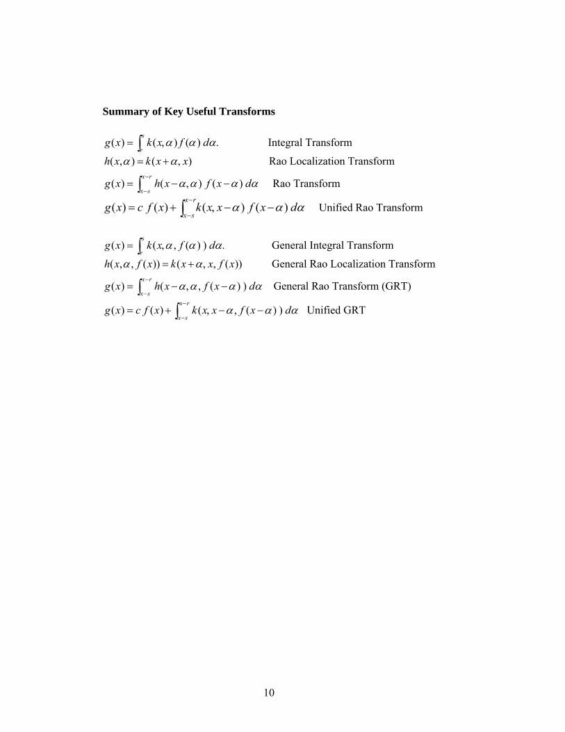
Summary of Key Useful Transforms

( ) ( ) ( )s

rg x k x f dα α α= , .∫ Integral Transform

( , ) ( )h x k x xα α= + , Rao Localization Transform

( ) ( ) ( )x r

x sg x h x f x dα α α α

−

−= − , −∫ Rao Transform

( ) ( ) ( ) ( )x r

x sg x c f x k x x f x dα α α

−

−= + , − −∫ Unified Rao Transform

( ) ( , ( ) )s

rg x k x f dα α α= , .∫ General Integral Transform

( , , ( )) ( , ( ))h x f x k x x f xα α= + , General Rao Localization Transform

( ) ( , ( ) )x r

x sg x h x f x dα α α α

−

−= − , −∫ General Rao Transform (GRT)

( ) ( ) ( , ( ) )x r

x sg x c f x k x x f x dα α α

−

−= + , − −∫ Unified GRT

11

Chapter I. A New Unified, Localized, and Computationally Efficient Approach to Integral Equations

“ [this research] has applications. It is guaranteed to produce doctoral dissertations.”

--An expert reviewer of this research for the U.S. Government, Feb. 2007. Overview A new approach is presented for solving integral equations. It is a fundamental computational and theoretical advance that provides a unified, fully localized, and computationally efficient solution in closed-form that is useful in both symbolic and numeric computations. The approach is naturally suited for fine-grain parallel implementation. In practical problems such as shift-variant image deblurring, the new approach offers significant computational speed-up in comparison with standard current techniques. Since Ordinary Differential Equations (ODEs) and Partial Differential Equations (PDEs) can be reformulated as integral equations by taking boundary conditions into account, the new approach is also relevant to solving ODEs and PDEs. It is also useful in image/signal filtering, and the analysis and modeling of linear and non-linear systems and processes, in engineering and applied sciences. 1. Linear Integral Equations Consider a conventional linear integral equation [2,3,4,] that includes Fredholm and Volterra Integral Equations of both the First and the Second Kind:

( ) ( ) ( ) ( )s

rg x c f x k x t f t dt= + ,∫ (0.1)

Here x and t are real variables, ( )f x is an unknown real valued function that we need to solve for, and ( )g x and ( )k x t, are known (or given) real valued functions. ( )k x t, represents the original integration kernel. For simplicity and without loss of generality, the conventional practice of using a factor λ (corresponding to an eigenvalue parameter) in front of the integral sign is not used here. r and s may be real constants (including possibly ±∞ ) or one of them can be the real variable x (they may also be known functions of x , but we shall not deal with this case here). c=0 for First Kind and c=1 for Second Kind integral equations. ( ) 0g x = for homogeneous integral equations. All functions here are assumed to be continuous, integrable, and differentiable up to some order as needed. The above integral equation will be restated in an equivalent form and without loss of any generality, using the change of variable

u x t= − . (1.2) A novel, unique, and innovative feature of this change of variable is that the new variable u is a function of both x and t instead of just t. This novel idea, although simple, has eluded researchers in the past, and it facilitates localizing the problem and deriving a closed-form solution. A more general change of variable such asu ax bt c= + + for real known constants a, b, and c (and other non-linear functions) are briefly considered later, but will not be considered here. With the above change of variable, we obtain

12

( ) ( ) ( ) ( )x s

x rg x c f x k x u f u du

−

−= + ,∫ (1.3)

which can be written as

( ) ( ) ( ) ( )x r

x sg x c f x k x x t f x t dt

−

−= + , − −∫ (1.4)

The above equation is named Rao Transform (RT) (of f(x) ) or Rao Integral Equation (RIE). It can be reduced to a differential equation as below:

0

0

( 1) ( ) (Taylor-series expansion)!

( ) ( 1) and )!

( ) ( ) ( ) ( )

( ) ( )

( ) ( ) (change order of

n nNn

nn

n nNn

nn

x r

x s

x r

x s

x r

x s

d f xtn dx

d f x tdx n

g x c f x k x x t f x t dt

c f x k x x t dt

c f x k x x t dt

=

=

−

−

−

−

−

−

⎛ ⎞−⎜ ⎟⎝ ⎠

−

= + , − −

≈ + , −

≈ + , −

∑

∑ ∑∫

∫

∫

∫

Therefore ( )

0( ) ( )( ) ( )

Nn

nn

k x f xg x c f x=

≈ +∑ (1.5)

where

( ) ( )

( 1)( )!

( )( )

( ) ,n

nn

nn n

n

x r

x sk x t

nd f xf f x

dx

k x x t dt−

−

−≡

≡ ≡

, −∫ (1.6)

In practical applications, both ( )nk x and ( )nf typically approach zero with increasing n. Let

( ) ( ) 0 for mf x m N= > . (1.7) Later we will consider the limit as N →∞ . Now, using suitable notation, we can derive from Eq. (1.5) an expression for the m-th order derivative of g(x) for m=0,1,2,…N, as:

( ) ( ) ( ) ( ) ( )

0 0

( )( ) ( ) ( ) ( )( )m N m

m m m m m p n pp nm

n p

d g xg g x C k x f x T n pdx

c f x − +

= =

≡ ≡ = ++ ∑∑

(1.8) where

( )( )

( )( ) ( )m p

m pn nm p

dk x k xdx

−−

−= (1.9)

and the function 1 for

( )0 otherwise.

n p NT n p

+ ≤⎧+ = ⎨

⎩ (1.10)

ensures that terms with ( ) ( )n pf x+ in Eq. (1.8) are set to zero when n p N+ > . Eq. (1.8) above can be simplified by grouping terms with respect to ( ) ( )nf x to obtain

( ) ( ) ( ),

0( ) ( ) ( ) for 0,1,2,( )

Nm m n

m nn

g x k x f x m Nc f x=

= =+∑ (1.11)

where

13

min( , )( )

,0

( ) ( )n m

m m pm n p n p

p

k x C k x−−

=

= ∑ . (1.12)

Equations (1.11) and (1.12) can be derived by noting the relation between the terms of ( ) ( )mg x derived from ( 1) ( )mg x− by applying the derivative operator for 1,2, ,m N= .

Eq. (1.11) can be written in vector-matrix form as: (0) (0) (0)

00 01 0(1) (1) (1)

10 11 1

( ) ( ) ( )0 1

1 0 00 1 0

0 0 1

N

N

N N NN N NN

g f fk k kk k kg f f

c

k k kg f f

⎡ ⎤ ⎡ ⎤ ⎡ ⎤⎡ ⎤⎡ ⎤⎢ ⎥ ⎢ ⎥ ⎢ ⎥⎢ ⎥⎢ ⎥⎢ ⎥ ⎢ ⎥ ⎢ ⎥⎢ ⎥⎢ ⎥= +⎢ ⎥ ⎢ ⎥ ⎢ ⎥⎢ ⎥⎢ ⎥⎢ ⎥ ⎢ ⎥ ⎢ ⎥⎢ ⎥⎢ ⎥⎢ ⎥ ⎢ ⎥ ⎢ ⎥⎣ ⎦ ⎣ ⎦⎣ ⎦ ⎣ ⎦ ⎣ ⎦

(1.13)

The above equation can be written in a more compact form using vector and matrix variables as:

( )x x x x xc= + =g I K f J f . (1.14) The subscript x in the above equation makes explicit the dependence of the vector/matrix on x. In this equation, note that the components of the column vectors are not the sampled values of g(x) and f(x) at different points x, but they are the different order derivatives of g(x) and f(x) at the same point x. Therefore, in practical applications, the size of the matrices will be small (3 to 6), but this matrix equation will have to be solved many times, once at value of x. At each point x, xg and xK will have to be computed from known data around the point x. We can obtain a symbolic solution for (0)( ) ( )f x f x= from Eq. (1.13) or (1.14) through a successive Gaussian elimination and back substitution method. This symbolic solution is useful in practical applications as the value of N is typically very small, around 3 to 6. Assuming that the matrix ( )x xc= +J I K is non-singular, the solution can be written in matrix form as:

1x x x x x

− ′= =f J g K g (1.15)

In explicit algebraic form, denoting the elements of 1

x x− ′=J K by ijk ′ , we may write the

solution as (0) (0) ( ) ( )

0 00 0

( ) ( ) lim ( ) ( ) ( ) ( )N N

n nn nN n n

f f x f x k x g x k x g x→∞

= =

′ ′= = = ≈∑ ∑ (1.16)

In practical applications, in order to reduce the effects of noisy data on the solution, a

regularization technique can be used to solve for xf . For example, a spectral filtering technique based on the Singular Value Decomposition (SVD) of

( )x xc= +J I K such as the Truncated SVD or Tikhonov regularization [6] can be used.

14

See later chapters for more details on extension of this approach to multi-dimensional cases and specific application examples, including two-dimensional shift-variant image deblurring. This approach is an extension of the author’s work on depth-from-defocus in computer vision [5]. 2. Non-linear Integral Equations A class of non-linear integral equations is represented by

( ) ( ) ( , ( ) )s

rg x c f x k x t f t dt= + ,∫ . (2.1)

Using the same change of variableu x t= − , the above equation can be written as:

( ) ( ) ( , ( ) )x r

x sg x c f x k x x t f x t dt

−

−= + , − −∫ (2.2)

The method of solution in this case is similar to that of linear integral equations described earlier up to the step of deriving expressions for the derivatives of g(x) up to order N. Then the next step will be to solve a system of non-linear algebraic equations, which is, in general, complicated. Some details on this problem can be found in later chapters [1].

3. Differential Equations Ordinary Differential Equations (ODEs) and Partial Differential Equations (PDEs) can be reformulated as integral equations by taking boundary conditions into account [2,3,4]. Solving such integral equations using the new approach presented here will solve the ODEs and PDEs. 4. Advantages The new approach provides a localized solution in the following sense—the solution

( )f x at a point x is expressed in terms of the values of the known function ( )g x at the same point x, and also the characteristics (or moments with respect to α) of the localized kernel at the same point x. In problems such as shift-variant image deblurring, this facilitates rapid convergence and accuracy of the series expansion in Eq. (1.16) that provides the solution. For the same reason, it permits a fine-grain parallel computation. The solutions at different points x can be computed in parallel using local data of the observed/measured function g(x) (whose local derivatives are used). At each point x, elements of a small (3x3 to 6x6 in practice, depending on data noise and solution accuracy) matrix xJ are computed and inverted. In practical applications, this matrix xJ often has a very simple form and can be computed very efficiently. For example, in shift-variant image deblurring, it is upper triangular and can be computed fast, either using analytic expressions, or, because the kernel is symmetric, i.e. ( , ) ( , )k x x t k x x t− = + , and has compact support with respect to t, i.e. it satisfies the condition ( , ) 0k x x t− = for | |t A≥ for some constant A which is much smaller than the size of the domain of integration (this is the case when the blurring model is based on geometric optics).

The solution at each point x will be compatible with the solutions at near-by points (up to some order derivatives of the solution). Therefore the local solutions can all be synthesized seamlessly (without glitches or discontinuities) at the borders (e.g. image deblurring) to obtain a global solution to the original problem. The new method provides

15

an analytic solution suitable for both theoretical analysis and numerical implementation. It provides a unified theory and a unified computational framework for a large and diverse class of both linear and non-linear integral equations. Numerical methods based on the new method are likely to offer significant computational savings [1]. The new approach can be naturally extended from one-dimensional to multi-dimensional problems. An important future research topic is to compare the computational performance of the new approach and its variations (e.g. incorporating TSVD or Tikhonov regularization) with existing approaches in practical applications.

5. References 1. "Rao Transforms: Theory and Applications", M. SubbaRao, U.S. Copyright

Registration No. TX 6-195-821, June 1, 2005. Self-published book, 120 pages. Purchase at http://www.integralresearch.net.

2. Kanwal, R. P., Linear Integral Equations: Theory and Technique, (2nd Ed.), Birkhauser Publishers, Boston, 1997, ISBN 0-8176-3940-3.

3. M. Masujima, Applied Mathematical Methods in Theoretical Physics, WILEY-VCH Verlag GmbH & Co. KGaA, Weinheim, 2005. ISBN 3-527-40534-8.

4. Polyanin, A. D., and Manzhirov, A. V., Handbook of Integral Equations, Boca Raton, FL: CRC Press, 1998.

5. M. Subbarao and G. Surya, "Depth from Defocus: A Spatial Domain Approach," International Journal of Computer Vision, Vol. 13, No. 3, pp. 271-294, 1994.

6. P. C. Hansen, J.G. Nagy, and D. P. O’Leary, “Deblurring Images: Matrices, Spectra, and Filtering”, book published by SIAM, 2006, ISBN 0-89871-618-7.

16

Chapter II Rao Transforms: A New Approach to Integral and Differential Equations

"In Mathematics, sometimes, the simplest results are the most useful results.” -- A Professor of Mathematics in his comments on this research.

1. Summary Rao Transforms (RTs) provide a brand new approach to the century old problem of solving linear and non-linear integral equations. The solution is completely localized and therefore permits extremely fine-grained parallel implementation on a computer. The approach is simple (easy to implement and comprehend) and unified as it solves a large class of diverse problems. Therefore RTs have both computational and theoretical advantages in practical applications. RTs are also useful in solving differential equations (DEs) as both ordinary and partial differential equations (ODE/PDEs) can be converted to integral equations that incorporate boundary conditions. Since many fundamental laws of physics are stated using ODE/PDEs, RTs are expected to have wide applications in science and engineering. The Rao Transform (RT) theory for solving linear integral equations can be summarized as follows. ( , ) ( )h x k x xα α= + , defines Rao Localization Transform/Equation (RLT/RLE). It transforms a conventional integration kernel ( , )k x α which is a “global form” description of the kernel into ( , )h x α which is a “local form” description of the kernel. This transformation can be used to define a Rao Transform (RT) or Rao Integral

Equation (RIE) as ( ) ( ) ( )x r

x shg x x f x dα α α α

−

−= − , −∫ which is, according to Rao’s First

Theorem (RFT), exactly equivalent to a conventional Integral Equation (IE) or Integral

Transform (IT) of the type ( ) ( ) ( )s

rkg x x f dα α α= ,∫ . In these equations, r and s may be

constants or one of them can be equal to the variable x. A unified, analytic, and localized (and therefore computationally efficient, accurate, and permits fine-grain parallel implementation) solution of RIE (and therefore the IE) can be obtained as follows. First, in the RT defined above, substitute truncated Taylor series expansions of ( )h x α α− , around ( )x α, and ( )f x α− around x , and simplify to obtain a series expansion of ( )g x in terms of the derivatives of ( )f x and moments of derivatives of ( )h x α, . Next, derive a system of linear algebraic equations by taking the derivatives of ( )g x upto a required order. Finally, solve this system of equations by a simple and efficient back/recursive substituition method. The resulting solution appears to be both theoretically and computationally superior to classical solutions provided by Fredholm’s determinants, Volterra’s iterated kernels, and orthonormal series expansions. Numerically, the new solution method is thought to be comparable or superior to classical techniques such as Collocation methods, Galerkin methods, and Nystrom methods. In particular, the new solution method is non-iterative and the computations are highly localized, thus making it ideal for implementation on massively parallel/distributed computing hardware. The results of RTs for linear integral equations can be extended to non-linear integral equations with similar advantages. In this case, a conventional “global form” kernel

17

( , , ( ))k x fα α is transformed to a “local form” kernel ( , , ( ))h x f xα by defining ( , , ( )) ( , ( ))h x f x k x x f xα α= + , .

Rao Transforms are an extension of the Spatial-Domain Convolution/Deconvolution Transoform (S Transform) invented about 15 years ago by this author. S transform has proved to be superior to the Fourier transform in some image processing and computer vision applications such as image restoration/filtering and depth-from-defocus. Rao Transforms are expected to have both theoretical and computational advantages similar to S transform in comparison with conventional methods for solving integral equations. 2. Background A Spatial-domain Convolution/Deconvolution Transform or S Transform was invented by this author in 1989 for the restoration of defocused images [1,2,7,15]. It provided a direct and localized spatial-domain method as opposed to the conventional Fourier domain method for image deconvolution, or the solution of a Convolution Integral Equation (CIE). CIE is a special case of the Fredholm Integral Equation of the First Kind where the integration kernel is shift-invariant. During the last 15 years, the practical applications and advantages of S transform has been successfully demonstrated for image restoration, depth-from-defocus, and autofocusing problems in modern digital cameras [2,7]. In particular, S transform based methods have been demonstrated to be superior to the Fourier transform based methods for depth-from-defocus and autofocusing applications, both in terms of computational speed and the accuracy of depth recovery and autofocusing. The main reason for this better performance seems to be that while inverse S transform provides local deconvolution, inverse Fourier transform provides global deconvolution. In the Summer of 2004, Rao Transforms [1,16,17] were invented by this author. Initially, Rao Transforms were derived by extending the S transform to solve the linear shift-variant image restoration or deblurring problem. In this case, the blurring kernel varies with image position, i.e. the kernel is shift-variant. This problem is the same as the problem of solving the Fredholm Integral Equation of the First Kind. A search of the research literature revealed that Rao Transforms were novel. In addition, it was found that Rao Transforms could be generalized to solve a large class of both linear and non-linear integral equations including Fredholm type, Volterra type, Urysohn type, Hammerstein type, etc. Since Ordinary Differential Equations (ODEs) and Partial Differential Equations (PDEs) can be reformulated as Integral Equations by taking boundary conditions into account, Rao Transforms are also relevant to solving ODEs and PDEs. The theoretical and computational advantages of S transform are expected to carry over to Rao Transforms in solving integral and differential equations as the two transforms are related. 3. Current State of the Art In the current research literature [4,5,6,8,9,10,11,12], there is no unified theory for solving general integral equations. Solution methods for different cases are disconnected, lacking a common theoretical or computational framework. The computational requirements of many solution methods are so large that they are of little use in practical

18

applications. Fredholm’s method of determinants and Volterra’s method of iterated kernels are two examples. Some solution methods rely on numerical and iterative techniques that contribute little towards a theoretical understanding of the problem. Three examples are Galerkin, Collocation, and Nystrom methods. Numerical stability and accuracy of solutions are two desirable characteristics lacking in many methods. Methods based on ortho-normal series expansions may fall into this category. An international expert and a program director of a US federal research funding agency reviewed a brief preliminary proposal on RTs. During the review process, he offered his expert opinion on the unsatisfactory state of the current state of the art in solving integral equations as follows:

"Numerical analysts hate solving integral equations because the resulting matrix approximations are usually full. This means that it takes O(n^2) operations to evaluate a matrix vector multiply and this is too much for large n. To get around this, applied mathematicians have looked for transformations which increase the sparsity of the matrix. Unfortunately, these type of transformations only work for matrices with special structure. The classical example is the Fourier transformation which reduces a circulant matrix to a diagonal matrix. These ideas go back at least to Cauchy. Recent examples are the Fast Multipole algorithm and some Wavelet transforms that I haven't paid much attention to. These methods are wonderful if your application has the right structure and are useless if they don't. [My agency] seems to mostly have problems in the category for which these methods are useless."

Clearly, the current state of the art is unsatisfactory. A quick search of literature revealed that Multipole algorithms and Wavelet transforms were not directly relevant to RTs. After a careful review of the brief preproposal, RTs were thought to be promising and a full proposal was invited. The full proposal received a very good technical review:

“In summary the proposed research appears to be valid and has applications. It is guaranteed to produce doctoral dissertations.”

4. Advantages of Rao Transforms Rao Transforms [1] provide a localized (permitting very fine-grain parallel implementation) analytic solution suitable for both theoretical analysis and numerical implementation. They provide a unified theory and a unified computational framework for a large class of both linear and non-linear integral equations. Numerical methods based on RTs are likely to offer significant computational savings. RTs can be naturally extended from the case of one dimensional problems to multi-dimensional cases. They can also be extended to linear combinations of standard form integral equations, and systems of simultaneous integral equations. Since RTs are novel, their complete list of advantages and disadvantages are yet to be determined through further research.

5. Rao Transform Theory Early results on the basic theory of RTs and their application to solve a large class of linear/non-linear integral/integro-differential equations including many classical

19

equations (e.g. Fredholm, Volterra, Urysohn, and Hammerstein) were presented in the First Edition of this book [1]:

M. Subbarao (Rao), Rao Transforms: Theory and Applications, U.S. Copyright Registration No. TX 6-195-821, June 1, 2005, self-published book, 120 pages, can be purchased at http://www.integralresearch.net.

This book is an updated version of the above book with new material in Chapters 1 and 2.

5.1 Rao Transform (RT) and General Rao Transform (GRT) The basic ideas underlying Rao Transform theory is introduced here with an example of a linear integral equation involving one-dimensional real valued variables and functions. These ideas can be extended to non-linear and multi-dimensional cases as in the book listed above [1]. First we state some of the main RTs:

( ) ( ) ( )s

rg x k x f dα α α= ,∫ Integral Transform/Equation (IT/IE) (1)

( , ) ( )h x k x xα α= + , Rao Localization Transform/Equation (RLT/RLE) (2)

( ) ( ) ( )x r

x sg x h x f x dα α α α

−

−= − , −∫ Rao Transform (RT) /

Rao Integral Equation (RIE) (3)

Here x and α are real variables, ( )f x is an unknown real valued function that we need to solve for, ( )g x , ( )k x α, , and ( )h x α, are known (or given) real valued functions. r and s may be real constants or one of them can be the real variable x . All functions here are assumed to be continuous, integrable, and differentiable. ( )k x α, and ( )h x α, are referred to as global and local kernel functions respectively. Using this notation and taking some liberty to use ambiguous notation (regarding g) and language in the interest of brevity, a crucial theorem is presented below.

Rao’s First Theorem (RFT): If ( )h x α, is defined as in Eq. (2) above (i.e. RLT is true), then IT in Eq. (1) and RT in Eq. (3) above are exactly equivalent with no loss of generality, i.e. ( )g x and ( )f x in the two equations are the same. Proof: R.H.S. of RT (Eq. 3) =

=

=

( ) ( )

(( ) ( )) ( ) from Eq. (2)

( ) ( )

x r

x sx r

x sx r

x s

h x f x d

k x x f x d

k x x f x d

α α α α

α α α α α

α α α

−

−−

−−

−

− , −

− + , − −

, − −

∫∫∫

Change the variable of integration to β where , and .x d dβ α β α= − = −

The new limits of integration are ,x s s x r rα β α β= − ⇒ = = − ⇒ = Therefore,

20

R.H.S. of RT (Eq. 3) =

=

R.H.S. of IT (Eq. 1).

( ) ( )

( ) ( )

=

s

rs

r

k x f d

k x f d

β β β

α α α

,

,

∫∫

The above theorem (RFT) is simple but has apparently eluded all the researchers so far, including Fredholm, Volterra, and Hilbert. This author derived it after he invented a new method for shift-variant image deblurring based on a Rao Transform and then tried to connect/relate his method to existing methods for solving integral equations. Rao Transform essentially restates, without loss of any generality, the same original problem of solving an integral equation in a localized form. In the new form, a localized solution can be obtained as follows:

( )

( )

0

( )

0

( )

0

( ) ( , ) ( )

( , ) ( ) (Taylor-series expansion)

( ) ( , )

( ) ( )

x r

x s

Nx r n nnx s

n

N x rn nn x s

n

Nn

n nn

g x h x f x d

h x a f x d

a f x h x d

a f x h x

α α α α

α α α α

α α α α

−

−

−

−=

−

−=

=

= − −

⎛ ⎞≈ − ⎜ ⎟

⎝ ⎠

≈ −

≈

∫

∑∫

∑ ∫

∑

where

( ) ( , )

( , ) ( )

x r nn x s

x r nnx s

h x h x d

k x x d k x

α α α α

α α α

−

−

−

−

≡ −

= − ≡

∫∫

.

Therefore, we may also write ( )

0( ) ( ) ( )

Nn

n nn

g x a f x k x=

≈ ∑ .

Let us define ( ) ( )( ) ( )( ) ( )

m mm mn n

n nm m

d h x d k xh x k xdx dx

≡ = ≡ .

We can derive an expression for the m-th derivative of g(x) (assuming that the m-th derivative of f(x) for m>N is zero) for m=0,1,2,…N, as:

( ) ( ) 0 for .mf x m N= >

21

( )

( )

( )

( ) ( )

0 0

( ) ( ), ,

0

( ) ( ), ,

0

( )( )

( ) ( )

( ) ( ) for 0,1, 2, ( ) ( )

( ) ( ) ( ) ( )

mm

m

N pmm n p m pp n n

p n

Nn m

m n m n nn

Nn m

m n m n nn

d g xg xdx

C a f x h x

h x f x m N h x h x

k x f x k x k x

−+ −

= =

=

=

≡

=

= = ≡

= ≡

∑ ∑

∑

∑

The above system of equations can be written in vector-matrix form as: (0) (0)

00 01 0(1) (1)

10 11 1

( ) ( )0 1

N

N

N NN N NN

g fh h hh h hg f

h h hg f

⎡ ⎤ ⎡ ⎤⎡ ⎤⎢ ⎥ ⎢ ⎥⎢ ⎥⎢ ⎥ ⎢ ⎥⎢ ⎥=⎢ ⎥ ⎢ ⎥⎢ ⎥⎢ ⎥ ⎢ ⎥⎢ ⎥⎢ ⎥ ⎢ ⎥⎣ ⎦⎣ ⎦ ⎣ ⎦

or (0) (0)

00 01 0(1) (1)

10 11 1

( ) ( )0 1

N

N

N NN N NN

g fk k kk k kg f

k k kg f

⎡ ⎤ ⎡ ⎤⎡ ⎤⎢ ⎥ ⎢ ⎥⎢ ⎥⎢ ⎥ ⎢ ⎥⎢ ⎥=⎢ ⎥ ⎢ ⎥⎢ ⎥⎢ ⎥ ⎢ ⎥⎢ ⎥⎢ ⎥ ⎢ ⎥⎣ ⎦⎣ ⎦ ⎣ ⎦

The above equation can be written in a more compact form using vector and matrix variables as:

or x x x x x x= =g H f g K f . The subscript x in the above equation makes explicit the dependence of the variables on x. We can obtain a symbolic solution for (0)( ) ( )f x f x= through recursive substitution or successive elimination as in Gaussian elimination. This symbolic solution is useful in practical applications as the value of N is very small, typically 2 to 6. Assuming that the matrix xH (or xK ) is non-singular, the solution can be written in matrix form as:

1 1f or fx x x x x x− −= =H g K g

In explicit algebraic form, we may write ( ) ( )

0 0( ) ( ) ( ) ( ) ( )

N Nn n

n n n nn n

f x a g x h x a g x k x= =

′ ′≈ =∑ ∑

We can define a resolvent kernel h’ (or k’) which is determined by 1x−H (the inverse of

xH , or 1x−K the inverse of xK ) so that the following equation is satisfied in the limit as

.N → ∞ :

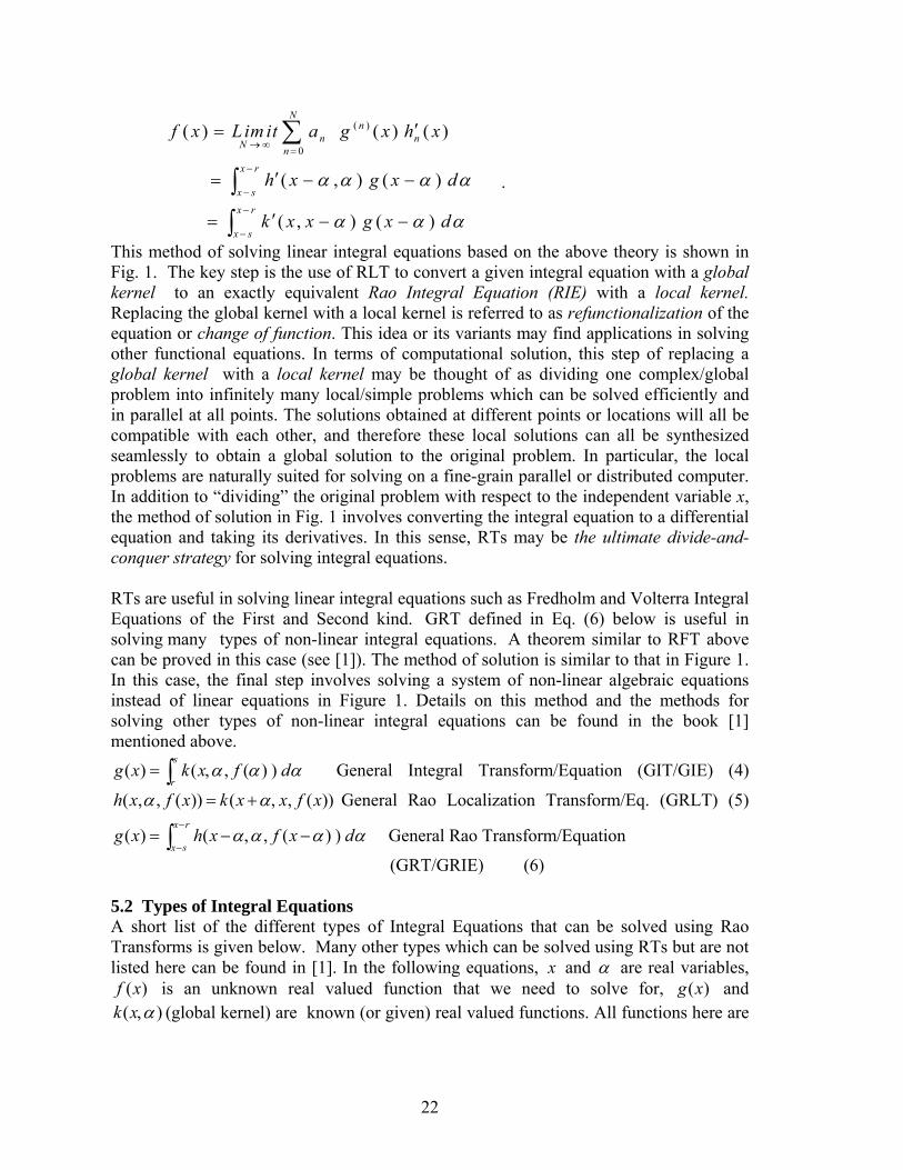
22

( )

0( ) ( ) ( )

( , ) ( )

( , ) ( )

Nn

n nN n

x r

x s

x r

x s

f x L im it a g x h x

h x g x d

k x x g x d

α α α α

α α α

→∞ =

−

−

−

−

′=

′= − −

′= − −

∑

∫∫

.

This method of solving linear integral equations based on the above theory is shown in Fig. 1. The key step is the use of RLT to convert a given integral equation with a global kernel to an exactly equivalent Rao Integral Equation (RIE) with a local kernel. Replacing the global kernel with a local kernel is referred to as refunctionalization of the equation or change of function. This idea or its variants may find applications in solving other functional equations. In terms of computational solution, this step of replacing a global kernel with a local kernel may be thought of as dividing one complex/global problem into infinitely many local/simple problems which can be solved efficiently and in parallel at all points. The solutions obtained at different points or locations will all be compatible with each other, and therefore these local solutions can all be synthesized seamlessly to obtain a global solution to the original problem. In particular, the local problems are naturally suited for solving on a fine-grain parallel or distributed computer. In addition to “dividing” the original problem with respect to the independent variable x, the method of solution in Fig. 1 involves converting the integral equation to a differential equation and taking its derivatives. In this sense, RTs may be the ultimate divide-and-conquer strategy for solving integral equations. RTs are useful in solving linear integral equations such as Fredholm and Volterra Integral Equations of the First and Second kind. GRT defined in Eq. (6) below is useful in solving many types of non-linear integral equations. A theorem similar to RFT above can be proved in this case (see [1]). The method of solution is similar to that in Figure 1. In this case, the final step involves solving a system of non-linear algebraic equations instead of linear equations in Figure 1. Details on this method and the methods for solving other types of non-linear integral equations can be found in the book [1] mentioned above.

( ) ( , ( ) )s

rg x k x f dα α α= ,∫ General Integral Transform/Equation (GIT/GIE) (4)

( , , ( )) ( , ( ))h x f x k x x f xα α= + , General Rao Localization Transform/Eq. (GRLT) (5)

( ) ( , ( ) )x r

x sg x h x f x dα α α α

−

−= − , −∫ General Rao Transform/Equation

(GRT/GRIE) (6) 5.2 Types of Integral Equations A short list of the different types of Integral Equations that can be solved using Rao Transforms is given below. Many other types which can be solved using RTs but are not listed here can be found in [1]. In the following equations, x and α are real variables,

( )f x is an unknown real valued function that we need to solve for, ( )g x and ( )k x α, (global kernel) are known (or given) real valued functions. All functions here are

23

D erive E quivalen t In tegral E quation using R ao T ransform

S im plify. G roup term s based on derivatives o f .

U n k n ow n F u n ction

( ) ( ) ( )x r

x sg x h x f x dα α α α

−

−= − , − .∫

S ubstitu te truncated T aylor-series ex pansions fo r around and a round .x( )f x α−( )x α,( )h x α α− ,

T ake derivatives w ith respect to x and derive asystem of at least N algebraic eqns in N unknow ns and so lve them bysim ple back-substitu tion .

( )nf

C onven tional L inear In tegralE quation w ith term s

A pp ly R ao Localization T ransform

( , ) ( )h x k x xα α= + ,

D ifferen tial E quation O D E /P D E+ B oundary C onditions

( )f x

( ) ( ) ( )s

rg x k x f dα α α= ,∫

( )nf

O RO R

( )f xS olu tion

( )f x

Rao Transforms: A New Approach to Integral and Differential Equations

Figure 1. Solving Linear Integral and Differential Equations

24

assumed to be continuous, integrable, and differentiable. nc , a, and b, all denote real

constants (possibly infinity), and ( )nf denotes the n-th derivative of f(x) at x with respect to x.

1. Fredholm Integral Equation of the First Kind ( ) ( ) ( )b

ag x k x f dα α α= ,∫

2. Fredholm Integral Equation of the Second Kind ( ) ( ) ( ) ( )b

ag x f x k x f dα α α= + ,∫ .

3. Volterra Integral Equation of the First Kind ( ) ( ) ( )x

ag x k x f dα α α= ,∫

4. Volterra Integral Equation of the Second Kind ( ) ( ) ( ) ( )x

ag x f x k x f dα α α= + ,∫

5. Urysohn Integral Equation of the First Kind ( ) ( , ( ))b

ag x k x f dα α α= ,∫

6. Urysohn Integral Equation of the Second Kind ( ) ( ) ( , ( ))b

ag x f x k x f dα α α= + ,∫

7. Urysohn-Volterra Integral Equation of the First Kind ( ) ( , ( ))x

ag x k x f dα α α= ,∫

8. Urysohn-Volterra Integral Equation of the Second Kind

( ) ( ) ( , ( ))x

ag x f x k x f dα α α= + ,∫

9. Linear integro-differential equations (Fredholm Type)

( )

0

( ) ( ) ( ) ( )N bn

n an

g x c f x k x f dα α α=

= + ,∑ ∫

10. Linear integro-differential equations (Volterra Type)

( )

0

( ) ( ) ( ) ( )N xn

n an

g x c f x k x f dα α α=

= + ,∑ ∫

When any integral equation expressed in a conventional form such as above is expressed in an equivalent localized form using RFT and RLT, then the resulting equation is referred to as the Rao Type Integral Equation (RTIE). 6. Example: Restoration of Shift-Variant Blurred Images 6.1 Summary A simple and easily verifiable example of the theory and application of RTs is presented here. A practical problem in shift-variant image restoration is considered which involves solving a Fredholm Integral Equation of the First Kind. A solution based on RTs is shown to provide a closed-form expression which is theoretically novel and interesting. This theoretical result is shown to extend to all linear integral equations in [1]. Similar ideas are used to derive the solution of non-linear integral equations as the solution of a set of non-linear algebraic equations in [1]. Computationally, the solution provided by the RTs for the example considered here is estimated to be about 1000 times faster for an image row with 1000 pixels compared to a conventional method of image restoration based on Singular Value Decomposition (SVD [3,14]) by inverting a large (1000x1000) matrix. This computational advantage is shown to extend to the special case of shift-invariant image blurring where a convolution integral equation is solved. In this special

25

case, the computational advantage is comparable to the famous Fast Fourier Transform (FFT) algorithm. If this computational advantage extends to the general integral equations which can be solved by RTs, a possibility in at least some cases, it would be a remarkable result. Further research is needed to confirm or contradict this possibility. As differential equations can be solved by reformulating them as integral equations [5,11], RTs are relevant to solving them as well. 6.2 Shift-variant Image Restoration We describe here a concrete one-dimensional example of the application of Rao Transforms. One practical problem for which this example is relevant is the restoration or deblurring of shift-variant motion blurred images. When a photograph is captured by a moving camera with a finite exposure period, say 0.1 second, objects nearer to the camera will have larger motion blur than farther objects. This situation can arise when the camera is on a moving platform such as a car or a robot. A similar situation, i.e. a shift-variant defocus blur, can arise in a laser barcode scanner for one-dimensional barcodes. When the plane of the barcode is slanted instead of being perpendicular to the direction of scan/view, the barcode image will be blurred by a shift-variant point spread function. Let the original focused image be f(x), and the corresponding blurred image be g(x). The conventional image blurring model in this case uses a shift-variant point spread function or kernel ( , )k x α . The blurred image g(x) and the kernel ( , )k x α are assumed to be given and the problem is to solve for the focused image f(x). The conventional blurring model is an integral equation of the form: ( ) ( , ) ( )g x k x f dα α α∞

− ∞= ∫ (6.1)

It is a one-dimensional Fredholm Integral Equation of the First Kind. The above model of blurring has two problems. First, it is difficult to find a closed-form inversion formula that is explicit and numerically stable. For example, the well-known Singular Value Decomposition (SVD) [3,14] technique is computationally expensive and unstable. Second, the above model does not capture the physical blurring process in a natural way. It seems to impose mathematical simplicity at the cost of direct natural modeling of the physical blurring process. We model the blurred image g(x) measured at x as the sum or integral over all possible point sources of the contribution due to each point source located at x-α. The contribution is given by the product of the strength of the signal point source f(x-α) and the value of a new localized shift-variant point spread function ( , )h x α α− . The new model of blurring is: ( ) ( , ) ( )g x h x f x dα α α α

∞

−∞= − −∫ (RT) (6.2)

where ( , ) ( )h x k x xα α= + , and (RLT) (6.3) ( ) ( )k x h xα α α, = , − (IRLT) (6.4)

The new model above is an integral equation that is exactly equivalent to the original integral equation (6.1) (see RFT for proof). Equation (6.2) is referred to as the Rao

26

Integral Equation (RIE) and defines the Rao Transform (RT). Equation (6.3) defines the Rao Localization Transform (RLT). Now the m-th order partial derivative of h(x,α) at (x,α ) with respect to x is denoted by

( ) ( ) ( )( )m

m mm

h xh h xx

αα ∂ ,= , = .

∂ (6.5)

The n-th derivative of f(x) at x with respect to x will be denoted by

( ) ( ) ( )( )n

n nn

d f xf f xd x

= = . (6.6)

The n-th moment of the m-th derivative of h is defined by

( ) ( ) ( )( )m

m m nn n m

h xh h x dx

αα α∞

−∞

∂ ,= =

∂∫ (6.7)

Note that the derivative is with respect to x and the moment is with respect to α. The original signal f(x) will be taken to be smooth or analytic so that it can be expanded in a Taylor series. The Taylor series expansion of f(x-α ) around the point x up to order N is

( )

0( ) ( )

Nn n

nn

f x a f xα α=

− = ∑ (6.8)

where

( 1) n

nan−

=!

. (6.9)

The above equation is exact and free of any approximation error when f itself is a polynomial of degree less than or equal to N. In this case, the derivatives of f of order greater than N are all zero. When f has non-zero derivatives of order greater than N, then the above equation will have an approximation error corresponding to the residual term of the Taylor series expansion. This approximation error usually converges rapidly to zero as N increases. In the limit as N tends to infinity, the above series expansion becomes exact and complete. Similarly, the Taylor series expansion of h(x-α, α) around the point (x,α) up to order M is

( )

0

( ) ( )M

m mm

m

h x a h xα α α α=

− , = ,∑ (6.10)

where ma are as in Eq. (6.9). Using a truncated Taylor series expansion as above gives very accurate approximations in many practical applications. One such example is image deblurring. In this case the kernel function usually changes smoothly and slowly with respect to x. If an analytic expression is given for h(x,α), then it may be possible to avoid the approximation introduced by truncation of the Taylor series above in Eq. (6.10). In this case, we would substitute Eq. (6.8) and the following analytic expression in Eq. (6.2) directly for obtaining a series expression for RT: ( ) ( )n

nh x h x dα α α α∞

−∞= − ,∫ .

Let N=2 and M=1, and let the original global kernel ( )k x α, be a Gaussian, that is

27

2

2

1 ( )( ) exp2 ( )2 ( )xk x αασ απσ α

⎛ ⎞−, = −⎜ ⎟

⎝ ⎠ (6.11)

where exp( ) xx e= . The kernel above is a “global” kernel. It is localized using the Rao Localization Transform (RLT) to define a new “local” kernel h as in Eq. (6.3), i.e.

( , ) ( )h x k x xα α= + , , which becomes 2

2

1( ) exp2 ( )2 ( )

h xxx

αασπσ

⎛ ⎞, = −⎜ ⎟

⎝ ⎠ (6.12)

For notational convenience, we denote

1( )( )

xx

ρσ

= . (6.13)

Therefore 2 2( ) ( )( ) exp

22x xh x ρ α ραπ

⎛ ⎞, = −⎜ ⎟

⎝ ⎠ (6.14)

The Taylor series expansion of ( )h x α α− , around the point ( )x α, up to order 1M = is ( 0 ) (1)( ) ( ) ( ) ( )h x h x h xα α α α α− , = , + , − . (6.15)

It can be shown that, when h is as defined in Eq. (6.14),

( )(1) 2 2( )( , )( , ) ( , ) 1 ( )( )

x xh xh x a h x xx x

ρα α α ρρ

∂= = −

∂ (6.16)

where ( )x xρ is the derivative of ( )xρ with respect to x. Note that the above function is an even function of α as it involves only α2. This function is symmetric with respect to α, i.e. h(1)(x, α ) = h(1)(x,-α). Therefore, all odd moments of h(1) with respect to α will be zero, and with M=1 and N=2, the RT becomes

2

( 0 ) (1) ( 2 ) ( 0 ) (1)( ) ( ) ( )2

g x f f f h h dαα α α∞

−∞= − + − .∫ (6.17)

Simplifying, we get

( 0 ) ( 0 ) ( 0 ) (1) (1) (1) ( 0 ) ( 2 ) ( 0 ) (1)0 1 2 1 2 3

1( ) ( ) ( )2

g f h h f h h f h h= − + − + − (6.18)

Since all odd moments of h(0) and h(1) are zero, we set ( 0 ) (1) (1)1 1 3 0 .h h h= = = This

simplifies the problem. Further, we have for this case, ( 0 )0 1h = and both first (1)

0h and second (2)

0h (and all higher) derivatives of (0)0h are always zero. Also the first and higher

derivatives with respect to x of (0)1h , (1)

1h , (1)2h , and (1)

3h are all zero. Only the first derivative of (0)

2h may not be zero. It will be denoted by (1)2h . Significant simplification

of a mathematical problem such as here is likely in many practical applications. With the above simplifications, we get ( 0 ) ( 0 ) (1 ) (1 ) ( 2 ) ( 0 )

2 212

g f f h f h= + + (6.19)

Taking derivatives of the above equation once and twice, we get

28

(1) (1) ( 2 ) (1) ( 2 ) (1)2 2

12

g f f h f h= + + (6.20)

and ( 2 ) ( 2 )g f= . (6.21) We treat the above equations (6.19 to 6.21) as three linear algebraic equations in the three unknowns (0)f , (1)f , and (2)f . They can be easily solved through successive back substitution. In this particular example, which corresponds to a typical practical application, the process of solving becomes trivial. In a general case where the kernel is not symmetric, there will be a system of N linear equations in the N unknowns ( )nf . These equations can be solved symbolically/numerically by recursive substitution (e.g. Gaussian elimination) and back-substitution. In practical applications, N is very small, typically in the range 2 to 6, and so the computational requirement is limited. Here we solve for f(0) = f(x) to obtain

(0 ) (0 ) (1) (1) ( 2 ) (0 ) (1) (1)2 2 2 2

1( ) ( 3 )2

f x f g g h g h h h= = − − − ⋅ (6.22)

The solution above can be further simplified by noting that (0) 22 ( )h xσ= and ( )(1) 2 2 4

2 3

( ) ( )( ) ( ) 3 ( ) 2( ) ( )

x xx xh x x xx x

ρ ρσ ρ σρ ρ

= − = − (6.23)

In matrix notation, the forward and inverse RT for this case (Equations 6.19 to 6.22) can be written as

(0) (1) (0)(0)2 2

(1)(1) (1)2

(2) (2)

1 (1 2)0 1 (3 2)0 0 1

g h h fg h fg f

⎡ ⎤ ⎡ ⎤⎢ ⎥ ⎢ ⎥⎢ ⎥ ⎢ ⎥⎢ ⎥ ⎢ ⎥⎢ ⎥ ⎢ ⎥⎢ ⎥ ⎢ ⎥⎢ ⎥ ⎢ ⎥⎢ ⎥ ⎢ ⎥⎣ ⎦ ⎣ ⎦

⎡ ⎤/⎢ ⎥= /⎢ ⎥⎢ ⎥⎣ ⎦

(0) (1) (0)(0) (1) (1)

2 2 2 2(1)(1) (1)2

(2) (2)

1 (1 2)( 3 )0 1 (3 2)0 0 1

f h h h h gf h gf g

⎡ ⎤ ⎡ ⎤⎢ ⎥ ⎢ ⎥⎢ ⎥ ⎢ ⎥⎢ ⎥ ⎢ ⎥⎢ ⎥ ⎢ ⎥⎢ ⎥ ⎢ ⎥⎢ ⎥ ⎢ ⎥⎢ ⎥ ⎢ ⎥⎣ ⎦ ⎣ ⎦

⎡ ⎤− − / − ⋅⎢ ⎥= − /⎢ ⎥⎢ ⎥⎣ ⎦

Thus we have obtained (in Eq. 6.22) the Inverse Rao Transform (IRT) for a case that is useful in practical applications. It is a closed-form solution up to second order terms. Solution up to any order N can be obtained similarly. As mentioned earlier, both matrix equations above involve upper triangular square matrices. Therefore simple back-substitution can be used to obtain both the forward and the inverse Rao Transforms. Here a solution for f(x) is given in terms of the derivatives of g(x) at x, and moments with respect to α of derivatives with respect to x of the localized kernel h. In all our search of relevant research literature, we have never seen such a closed-from solution for the Fredholm Integral Equation of the First Kind. This is a “local” solution and converges rapidly for this particular example. In particular, unlike the conventional SVD method (3,14), the local solution above given by IRT can be implemented more easily on a parallel or distributed computer. The solution f(x) is computed for each different value of x separately and independently. A few other more complicated examples of solutions of

29

integral equations are presented in the book [1], but the simple example here illustrates the potential power of RTs. Note that, in the process of solving for f(x) at x, we also obtain solutions for (1)f , and

(2)f . Therefore, a Taylor series expansion as in Equation (6.8) can be used to extend the solution at x approximately to a small interval surrounding x. This extended solution will be exact for all α if f itself is a polynomial of order 2N ≤ globally. Otherwise, the accuracy of the solution for f(x-α) will decrease as α increases. 6.3 Computational Complexity Let a one-dimensional (1D) laser barcode scanner be characterized by a 1D Gaussian blurring kernel given by Eq. (6.11) or (6.12). Suppose that it is used to scan a two inch long barcode on a slanted plane at 1000 dots per inch resolution. Let the slant of the plane be such that the blur parameter σ increases smoothly from 1 pixel at the starting pixel to 10 pixels at the last pixel. These 1000 samples represent one row of the blurred image signal g(x) of size P=1000 pixels. Let the support size of the kernel h be s where s is defined as

( ) 0 fo r fo r a llh x s xα α α| − , | ≈ | | > . (6.24) A localized kernel that satisfies the above condition (6.24) is said to have a compact support. In our example, this s is roughly proportional (by a factor of 2) to the blur parameterσ and has a value in the range of 2 to 20 pixels. The value of s is typically 1 to 2 orders of magnitude smaller than P. Although closed-form expressions as in Eq. (6.23) may exist for computing the moments of the derivatives of the kernel when the kernel is a standard mathematical function such as a Gaussian, for a general kernel function ( )O s operations would be needed to compute these moments at each pixel x. A conventional method of restoring the above image is as follows. A discrete version of Equation (6.1) is written with uniformly sampled g(x) and f(x) represented by vectors of size 1000 and the kernel k by a 1000x1000 sampled matrix. A solution for f(x) is obtained by inverting the 1000x1000 matrix corresponding to the global kernel k. Inverting a PxP matrix has a computational complexity of 3( )O P which is very high for P=1000. In the presence of noise, a Singular Value Decomposition method may be used in practice. It is possible to solve this problem by considering small intervals at time, for example by dividing the 1000 pixel interval into 10 intervals of 100 pixel each, and solving the equation separately in each interval. In this case, the computational complexity would be

310 (100 ).O⋅ However, this approach will reduce the accuracy of the solution, especially at the end points of the intervals since blurred pixels just outside the interval will affect measured g(x) just inside the interval. In addition this approach permits only a very coarse grained parallel implementation on a computer. In the new method based on RT, the computational complexity is ( )O Pst operations where t is the highest order derivative considered in the local Taylor series expansion of f or g. In our blurring example, a typical value for t would be 4. Estimating the derivatives of g at each pixel x requires ( )O t operations using ( )O t data points. This t is typically 2 to 3 orders of magnitude smaller than P and a reasonable estimate may be

30

( ) (log )O t O P≤ . t is also the number of terms on the right hand side of inverse Rao Transform (in Eq. 6.22). Therefore the computational speed up is 2( /( ))O P st which is typically over ( )O P or 1000. The method can be implemented in parallel with one processor for each pixel operating on ( )O t data points of g(x) and ( )O s data points of the kernel ( ) fo r fo r a llh x s xα α α− , | | ≤ . In the limiting case when truncation of the Taylor series expansions are not permitted in order to preserve full accuracy, t=P. Note that a P-th order polynomial will fit the P data points of g which can be expanded in a Taylor series with P terms with no approximation, and therefore there will be P terms in the solution of f. In this case, solution of f and all its P derivatives at a single point x can be used to compute f at all possible points x using a Taylor series expansion as in Equation (6.8). As the interval of support s of the kernel h increases to span the entire space of P points where g is defined, s approaches P. In this worst case scenario, the computational complexity of the RT method equals that of the conventional method or the SVD method [3] which is 3( )O P . If the blurring kernel is a standard mathematical function, then ( )O s computational operations needed for computing the moments of the kernel h can be avoided because an analytic expression can be used to compute them. This offers significant additional computational advantage. It is interesting to note that when M=0 in Equation (6.10), the shift-variant blurring becomes shift-invariant which corresponds to a convolution operation. See Reference [2,7] for a practical application of this case. In this case, ( ) (1)O s O= because there is no need to re-compute the moments of h at each point x as they remain the same at all points. The moments of h need to be computed only once. Therefore the computational complexity of the proposed method becomes ( )O Pt . This compares very well with the Fast Fourier Transform (FFT) method which has a computational complexity of

( log )O P P . The computational speed up attained by RT as compared to FFT is (log / )O P t which may be significant in some practical applications (see [2]). Note that

while RT can be naturally extended to the shift-variant problems, FFT cannot be extended to them. In addition, RT permits a more fine-grain parallel implementation than the FFT. The example above is for a one-dimensional image. For an actual 2D image and other higher dimensional applications, the computational advantages would be much higher. In conclusion, Rao Transforms are theoretically interesting, and practically useful. Further research is needed to explore and exploit their full potential. 7. Solving Ordinary and Partial Differential Equations (ODEs/PDEs) A differential equation by itself is inherently under-constrained in the absence of initial values or boundary conditions. A differential equation along with the initial values or boundary conditions can be compactly and explicitly represented by an integral equation. In this integral representation, it becomes possible to solve the problem. It is said (e.g. [5]) that one of the most important achievements and applications of integral equation methods are in solving partial differential equations (PDEs) of second order, such as the Laplace ( 2 0f∇ = ), Poisson ( 2 4f gπ∇ = − ; g is a given function of position), and

31

Helmholtz (or the steady-state wave) ( 2 2( ) 0k f∇ + = ; k is a number) equations. Boundary value problems for elliptic type PDEs can be reduced to Fredholm integral equations, and parabolic and hyperbolic PDEs lead to Volterra integral equations. For these reasons, Rao Transforms as a tool for solving Integral Equations are directly relevant to solving ODEs and PDEs. This is an area that remains completely unexplored. Applying RTs to solve ODEs and PDEs may lead to fundamentally new approaches to problems in theoretical physics and mechanics. It may also lead to a big leap in computational techniques for solving boundary value problems in many applied sciences, from the design of submarine hulls and missiles [19] to inverse optics [18]. In order to see how the application of RTs may change a conventional technique for solving differential equations, we shall consider a simple example here. 7.1 Example: n-th order initial value problem Consider an n-th order linear differential equation and initial values:

( )

( )0

( ) ( ) ,n kn

k n kk

d yA x F xdx

−

−=

=∑ with (7.1)

( ) ( )n kn ky r q−−= as initial conditions for 0,1, , 1k n= − , (7.2)

where ,kA F are defined and continuous in the interval r x s≤ ≤ and kq are given constants. Assume, without loss of generality that 0 ( ) 1.A x = Define / ( )n ndy dx f x= . This initial value problem can be converted to the following Volterra Integral Equation of the second kind [5] (pages 62,63):

( ) ( ) ( , ) ( )x

rg x f x K x f dα α α= − ∫ , where (7.3)

1

1

( )( , ) ( )( 1)!

kn

kk

xK x A xkαα

−

=

−= −

−∑ and (7.4)

{ }1 1 1 2 2

11 1 0

( ) ( ) ( ) [( ) ] ( )

[( ) /( 1)!] ( ) ( )n n n

nn n

g x F x q A x x r q q A x

x r n q x r q q A x− − −

−−

= − − − + −

− − − + + − +. (7.5)

After solving the integral equation above for / ( )n ndy dx f x= , the solution for y can be obtained by integrating it n times as in [5]. The solution is given by

1 1

0

( ) ( )( ) ( )( 1)! !

n knx

krk

x x ry x f d qn kα α α

− −

=

− −= +

− ∑∫ . (7.6)

Applying the Rao Transform technique, we obtain the following equivalent Rao Type integral equation for the above Volterra Integral Equation of the second kind (7.3):

0( ) ( ) ( , ) ( )

x rg x f x H x f x dα α α α

−= − − −∫ , where (7.7)

1

1( , ) ( )

( 1)!

kn

kk

H x A xkαα α

−

=

= − +−∑ . (7.8)

Solution of the above integral equation is obtained by following steps similar to those in Figure 1. In short, expand ( , )H x α α− in a truncated Taylor series around the point ( , )x α , expand ( )f x α− in a truncated Taylor series around (x) , simplify the integral equation by grouping terms based on the derivatives of f with respect x , consider various

32

order derivatives of g with respect to x to obtain a system of linear algebraic equations, solve them through a successive elimination and back substitution procedure. The theoretical and computational advantages of this new method needs to be investigated as part of future research.

8. Future Research Topics Except for numerical stability and convergence characteristics of solutions, all other theoretical characteristics such as existence and uniqueness of solutions should be the same for both conventional integral equations (CIEs) and their equivalent Rao integral equations (RIEs). This is a consequence of the fact that the domain of definition of the kernels in the two cases are exactly the same. However, while rederiving existing theoretical results on CIEs for RIEs directly may not provide new results, such rederivations may be simpler/unifying which would reduce efforts in teaching/learning the subject matter, and perhaps provide new insights. Therefore such theoretical study would be of interest as a future research topic.

The most important achievements of Rao Transforms may not be that they provide unified theoretical and computational frameworks for solving a large class of integral equations, but it may be that they provide computationally more parallel, efficient, accurate, and stable results than current state-of-the-art methods, at least in some cases, particularly those cases which are of practical importance. Finding such cases where RTs have advantages and applying them would be a useful research topic.

Comparing the computational performance of RTs with current state-of-the-art methods should be a future research topic. Problems of practical importance in engineering (e.g. shift-variant image/signal restoration) and science (e.g. inverse optics, potential theory, initial/boundary value problems) should be investigated for solutions based on RTs. Relative performance of RTs in terms of computational resources used, accuracy, numerical stability, and convergence characteristics, need to be evaluated. Fast computational algorithms should be developed for RTs. Special attention should be paid to solving classical integral equations of Fredholm, Volterra, Urysohn, and Hammerstein types. Extension of Rao Transform theory to functions of complex variables, and extension to discrete or matrix equations are also future research topics of interest. For example, RT can be used to define the concept of “local eigen value/function” and the discrete version of Rao Transform equation can be used to define “local matrix/tensor” product. Presentation slides accompanying this report at www.integralresearch.net provide some additional details on this aspect. An expert reviewer of a research proposal based on RTs commented as follows on the overall potential of future research on RTs:

“If certain class of differential equations and boundary value problems could be solved more effectively, it is likely to have application in problems of computational and finite element fluid mechanics. Specifically could help in the hull design of underwater vehicles. Solving integral equation will also likely impact computational physics”.

33

Perhaps the latest book on integral equations is by Dr. Michio Masujima [8], a Mathematical Physicist from MIT. It was published in 2005, and according to the Preface there, it is based on courses on integral equations taught in the Department of Mathematics at MIT, and at Harvard. On the back cover of the book is the claim "All there is to know about functional analysis, integral equations, and calculus of variations in a single volume". On page 39 of the book we find the following discussion. It is in general easy to transform a differential equation into an integral equation but it says on page 39 “we never solve a differential equation by such a transformation.” It then continues “ Indeed, an integral equation is much more difficult to solve than a differential equation in a closed form. Only very rarely can this be done. Therefore, whenever it is possible to transform an integral equation into a differential equation, it is a good idea to do so [and solve it]”. It should be noted that RTs (always as opposed to rarely) transform an integral equation into a differential equation that is easily solved in closed-form using a truncated Taylor series expansion. Equation (6.18) is a simple example of such a differential equation. However, there is a crucial difference because a conventional differential equation uses boundary conditions specified as separate equations, but the differential equation derived by RT already includes the boundary conditions (see [1] for a more general example of applying RTs to solve a Volterra Integral Equation of the Second Kind). Further research is needed to investigate the relation between RTs and other conventional techniques for solving differential equations, e.g. the method of Green’s functions. 8.1 Generalization of Rao Transform Theory The theory of RTs can be generalized further, but its practical applications remain unexplored. One way to extend the RT theory is as follows. Consider the conventional integral equation:

( ) ( ) ( )s

rg x k x f dα α α= ,∫

In the above equation, note that integration is with respect to α, and therefore α is a dummy variable. It can be replaced by another suitable dummy variable β that is a function of both α and x defined by:

( , )xβ β α= . With this change of variable, the integral equation becomes:

( , )

( , )( ) ( ( , )) ( ( , ))

x s

x rg x k x x f x d

β

ββ α β α β= ,∫ .

A simple example of ( , )xβ α is: ( , )x a x b cβ α α= + + where a, b, and c are known scalar constants.

Note that setting 1a = , 1b = − , and 0c = results in the original definition of Rao Transforms where ( , )x xβ α α= − . In an extended theory of RTs, ( , )xβ β α= can be a very general function but satisfying appropriate properties (e.g., it should be uniquely invertible with respect to α, i.e. a one to one and onto function of α for all x). The case when ( , )xβ α is a general linear function of x and α as defined above may have some practical applications. Such a general linear function includes translation and scaling with

34

respect to x and α. Therefore, the effect can be thought of as positioning and scaling the problem as desired depending on the constants a, b, and c, instead of just localizing the problem as in RTs. In this case, the resulting integral equation can be solved easily by following steps similar to deriving the original inverse RT. In this case, the Taylor series expansion of ( )f ax b cα+ + can be done in two ways. The first way is in terms of the derivatives of ( )f ax c+ and powers of bα , and the second way is in terms of the derivatives of ( )f ax and powers of b cα + . The choice depends on the problem at hand. In both cases, this Taylor series expansion can be denoted symbolically as

( )( )

0( ( , )) ( )

Nn

n xn

f x a fβ α α=

≈∑ .

Therefore we can derive ( , )

( , )

( , ) ( )( )( , )

0

( , )( )( ) ( , )

0

( )( )

0

( ) ( , ( , )) ( ( , ))

( , ( , )) ( )

( ) ( , ( , ))

( )

x s

x r

Nx s nn xx r

n

N x snx nx r

n

Nn

x nn

g x k x x f x d

k x x a f d

f a k x x d

f k x

β

β

β

β

β

β

β α β α β

β α α β

α β α β

=

=

=

=

≈

≈

≈

∫

∑∫

∑ ∫

∑

where ( , )

( , )( ) ( ) ( , ( , ))

x s

n nx rk x a k x x d

β

βα β α β≡ ∫

In the above derivation, the key step is the factorization of the terms in the series expansion of ( ( , ))f xβ α where one term depends only on α and the other term depends only on x. After we derive the expression

( )( )

0

( ) ( )N

nx n

n

g x f k x=

≈∑ ,

the subsequent steps for solving for f(x) are similar to the original RT. They involve deriving expressions for derivatives of g(x) assuming

( )( ) 0 for mxf m N= >

and solving a system of linear equations. The above generalization of the RT theory for linear integral equations can be extended in a similar manner to the case of non-linear integral equations, and non-linear cases of

( , )xβ α . This generalization will be carried out as the practical need arises. 8.2 Discrete Case In the discrete case, using matrices, vectors, and integer index variables that correspond to the continuous case, we may write

[ ] [ ] [ ]s

r

g x k x fα

α

α α=

=

= ,∑

35

In the above equation, note that summation is done with respect to the index α. As summation can be done in any order as long as the terms of summation remain the same, we may use a new index of summation β that is a uniquely invertible function with respect to α of both α and x defined by:

[ , ]xβ β α= . The summation can be done in any order we desire by appropriately choosing the bijective mapping between α and β. Compare this with the continuous case where a small change in α corresponds to a small change in β. Now the summation becomes:

( , )

( , )

[ ] [ [ , ]] [ [ , ]]x s

x r

g x k x x f xβ

β β

β α β α=

= ,∑ .

Depending on the application, it may be possible to speed up the above summation, or equivalently a matrix-vector product computation, by appropriately choosing

[ , ]xβ β α= and grouping terms with common product terms, e.g. as in FFT computation. Speed-up is also possible if [ [ , ]]f xβ α can be expressed in a rapidly convergent series expansion (e.g. Taylor series) where the terms are separable with respect to x and α as:

[ ][ ]

0[ ( , )] [ ]

Nn

n xn

f x e fβ α α=

≈∑

In this case, computation is reduced by truncating the above series expansion. This is permissible provided the error is bounded and acceptable.

( , )[ ]

[ ]( , ) 0

( , )[ ]

[ ]0 ( , )

[ ][ ] [ ]

0

[ ]

[ ]

[ ]

[ ] [ [ , ]]

[ [ , ]]

x s Nn

x nx r n

x sNn

x nn x r

Nn

x nn

f e

f e

f k x

g x k x x

k x x

β

β β

β

β β

α

α

β α

β α

= =

= =

=

≈ ,

≈ ,

≈

∑ ∑

∑ ∑

∑

9. References 1. "Rao Transforms: Theory and Applications", by M. Subbarao (Rao), U.S.

Copyright Registration No. TX 6-195-821, June 1, 2005. Self-published book, 120 pages. Purchase at http://www.integralresearch.net.

2. M. Subbarao, T. Wei, and G. Surya,"Focused Image Recovery from Two Defocused Images Recorded with Different Camera Settings," IEEE Transactions on Image Processing , Vol. 4, No. 12, 16 pages, Dec. 1995.

3. A. K. Jain, Fundamentals of Digital Image Processing, Section 8.9, pages 299 to 301, Prentice-Hall, Inc., 1989, ISBN 0-13-336165-9.

4. Polyanin, A. D., and Manzhirov, A. V., Handbook of Integral Equations, Boca Raton, FL: CRC Press, 1998.

5. Kanwal, R. P., Linear Integral Equations: Theory and Technique, (2nd Ed.), Birkhauser Publishers, Boston, 1997.

6. K. E. Atkinson, The Numerical Solution of Integral Equations of the Second Kind, Cambridge University Press, 1997.

36

7. M. Subbarao and G. Surya, "Depth from Defocus: A Spatial Domain Approach," International Journal of Computer Vision, Vol. 13, No. 3, pp. 271-294, 1994.

8. M. Masujima, Applied Mathematical Methods in Theoretical Physics, WILEY-VCH Verlag GmbH & Co. KGaA, Weinheim, 2005. ISBN 3-527-40534-8.

9. Eric W. Weisstein. "Integral Equation." From Mathworld, A Wolfram Web Resource. http://mathworld.wolfram.com/IntegralEquation.html

10. Corduneanu, C. Integral Equations and Applications, Cambridge, England: Cambridge University Press, 1991.

11. Kondo, J. Integral Equations, Oxford, England: Clarendon Press, 1992. 12. Delves, L.M. and Mohamed, J.L. Computational Methods for Integral Equations,

Cambridge University Press, 1985. 13. M. Subbarao, “Passive ranging and rapid autofocusing,” U.S. patent No. 5,148,209,

Sept. 15, 1992. 14. W. K. Pratt, Digital Image Processing, Second Edition, Section 12.3, pages 376 to

382, John Wiley and Sons, 1991, ISBN 0-471-85766-1. 15. M. Subbarao, A method and apparatus for restoring convolution degraded images

and signals, U.S. patent application serial no. 07/548,287, filing date 07/03/90 (abandoned).

16. M. Subbarao (Rao), “Methods and apparatus for computing the input and output signals of a linear shift-variant system”, United States Patent and Trademark Office, Provisional patent application filed on 11/08/2004, Ref. No. 16800 U.S. PTO. 60/626028. Full patent application filed on 9/26/2005. No. 113010 U.S. PTO, 11/235724.

17. (a) M. Subbarao (Rao), “Method and Apparatus for Solving Linear and Non-Linear Integral and Integro-Differential Equations", United States Patent and Trademark Office, Provisional patent application filed ion 11/23/2004, Ref. No. 22151 U.S. PTO. 60/630395. Combined full patent application filed on 10/03/2005, No. 112991 U.S. PTO, 11/242191.

(b) M. Subbarao (Rao), “Unified Method and Apparatus for Solving Linear and Non-Linear Integral, Integro-Differential, and Differential Equations", Provisional patent application filed in the United States Patent and Trademark Office, 11/29/2004, Ref. No. 19249 U.S. PTO, 60/631555. Combined full patent application filed on 10/03/2005, No. 112991 U.S. PTO, 11/242191.

18. M. Subbarao (Rao), “Direct Vision Sensor for 3D Computer Vision, Digital Imaging, and Digital Video", Provisional patent application filed in the United States Patent and Trademark Office, June 18, 2005, Ref. No. 113013 U.S. PTO, 60/691358. Full patent application filed on 6/10/2006. No. 112959 U.S. PTO, 11/450024.

19. P. M. Guevel and P. R. Bardey, “Air or submarine engine with improved contour”, U. S. Patent No. 5024396, June 18, 1991.

37

Chapter III. Rao Transforms: Application to the Restoration of Shift-Variant Blurred Images

Introduction

We describe concrete one-dimensional (1D) and two-dimensional (2D) examples of the practical application of Rao Transforms (RTs) [1]. The one-dimensional example is relevant to the restoration or deblurring of shift-variant motion blurred images. When a photograph is captured by a moving camera with a finite exposure period, say 0.1 second, objects nearer to the camera will have larger motion blur than farther objects. This situation can arise when the camera is on a moving platform such as a car or a robot. A similar situation, i.e. a shift-variant defocus blur, can arise in a laser barcode scanner for one-dimensional barcodes. When the plane of the barcode is slanted instead of being perpendicular to the direction of view, the barcode image will be blurred by a shift-variant point spread function (SV-PSF). The two-dimensional example is related to the restoration of images (or signals) degraded by a SV-PSF, such as blurred images of a slanted plane or a curved surface produced by a defocused camera system.

One–Dimensional case Let the original focused image be f(x), and the corresponding blurred image be g(x). The conventional image blurring model in this case uses a shift-variant point spread function or kernel k(x, α). The blurred image g(x) and the kernel k(x, α) are assumed to be given and the problem is to solve for the focused image f(x). The conventional blurring model is an integral equation of the form: ( ) ( , ) ( )g x k x f dα α α∞

− ∞= ∫ (1)

It is a one-dimensional Fredholm Integral Equation of the First Kind. The above model of blurring has two problems. First, it is difficult to find a closed-form inversion formula that is explicit and numerically stable. For example, the well-known Singular Value Decomposition (SVD) technique is computationally expensive and unstable. Second, the above model does not capture the physical blurring process in a natural way. It seems to impose mathematical simplicity at the cost of direct natural modeling of the physical blurring process.

We model the blurred image g(x) measured at x as the sum or integral over all possible point sources of the contribution due to each point source located at x-α. The contribution is given by the product of the strength of the signal point source f(x-α) and the value of a new localized shift-variant point spread function h(x-α,α). The new model of blurring is:

( ) ( , ) ( )g x h x f x dα α α α∞

−∞= − −∫ (RT) (2)

where ( , ) ( )h x k x xα α= + , and (RLT) (3) ( ) ( )k x h xα α α, = , − (IRLT) (4)

The new model above is an integral equation that is exactly equivalent to the original integral equation (1) (see [1] for proof). Equation (2) is referred to as the Rao Integral

38

Equation (RIE) and defines the Rao Transform (RT). Equation (3) defines the Rao Localization Transform (RLT).

Now the m-th order partial derivative of h(x,α) at (x,α ) with respect to x is denoted by

( ) ( ) ( )( )m

m mm

h xh h xx

αα ∂ ,= , = .

∂ (5)

The n-th derivative of f(x) at x with respect to x will be denoted by

( ) ( ) ( )( )n

n nn

d f xf f xd x

= = . (6)

The n-th moment of the m-th derivative of h is defined by

( ) ( ) ( )( )m

m m nn n m

h xh h x dx

αα α∞

−∞

∂ ,= =

∂∫ (7)

Note that the derivative is with respect to x and the moment is with respect to α. The original signal f(x) will be taken to be smooth or analytic so that it can be expanded in a Taylor series. The Taylor series expansion of f(x-α ) around the point x up to order N is

( )

0( ) ( )

Nn n

nn

f x a f xα α=

− = ∑ (8)

where

( 1)n

nan−

=!

. (9)

The above equation is exact and free of any approximation error when f itself is a polynomial of degree less than or equal to N. In this case, the derivatives of f of order greater than N are all zero. When f has non-zero derivatives of order greater than N, then the above equation will have an approximation error corresponding to the residual term of the Taylor series expansion. This approximation error usually converges rapidly to zero as N increases. In the limit as N tends to infinity, the above series expansion becomes exact and complete.

Similarly, the Taylor series expansion of h(x-α, α) around the point (x,α) up to order M is

( )

0

( ) ( )M

m mm

m

h x a h xα α α α=

− , = ,∑ (10)

where ma are as in Eq. (9). Using a truncated Taylor series expansion as above gives very accurate approximations in many practical applications such as image deblurring as the kernel function usually changes smoothly and slowly with respect to x. Example(1): We conclude our one-dimensional discussion with a specific example where we let N = 2, M = 1, and let the original kernel k be a Gaussian, that is

39

2

2

1 ( )( ) exp2 ( )2 ( )xk x αασ απσ α

⎛ ⎞−, = −⎜ ⎟

⎝ ⎠ (11)

where exp( ) xx e= . The kernel above is a “global” kernel. It is localized using the Rao Localization Transform (RLT) to define a new “local” kernel h as in Eq. (3), i.e.

( , ) ( )h x k x xα α= + , , which becomes 2

2

1( ) exp2 ( )2 ( )

h xxx

αασπσ

⎛ ⎞, = −⎜ ⎟

⎝ ⎠ (12)

For notational convenience, we denote 1( )

( )x

xρ

σ= . (13)

Therefore 2 2( ) ( )( ) exp

22x xh x ρ α ραπ

⎛ ⎞, = −⎜ ⎟

⎝ ⎠ (14)

The Taylor series expansion of ( )h x α α− , around the point ( )x α, up to order 1M = is ( 0 ) (1)( ) ( ) ( ) ( )h x h x h xα α α α α− , = , + , − . (15)

It can be shown that, when h is as defined in Eq. (14),

( )(1) 2 2( )( , )( , ) ( , ) 1 ( )( )

x xh xh x a h x xx x

ρα α α ρρ

∂= = −

∂ (16)

where ( )x xρ is the derivative of ( )xρ with respect to x.

Note that the above function is an even function of α as it involves only α2. This function is symmetric with respect to α, i.e. h(1)(x, α ) = h(1)(x,-α). Therefore, all odd moments of h(1) with respect to α will be zero, and with M=1 and N=2, the RT becomes

2

( 0 ) (1) ( 2 ) ( 0 ) (1)( ) ( ) ( )2

g x f f f h h dαα α α∞

−∞= − + − .∫ (17)

Simplifying, we get

( 0 ) ( 0 ) ( 0 ) (1) (1) (1) ( 0 ) ( 2 ) ( 0 ) (1)0 1 2 1 2 3

1( ) ( ) ( )2

g f h h f h h f h h= − + − + − (18)

Since all odd moments of h(0) and h(1) are zero, we set ( 0 ) (1) (1)1 1 3 0 .h h h= = = This

simplifies the problem. Further, we have for this case, ( 0 )0 1h = and both first (1)

0h and second (2)

0h (and all higher) derivatives of (0)0h are always zero. Also the first and higher

derivatives with respect to x of (0)1h , (1)

1h , (1)2h , and (1)

3h are all zero. Only the first derivative of (0)

2h may not be zero. It will be denoted by (1)2h . Significant simplification

of a mathematical problem such as here is likely in many practical applications. With the above simplifications, we get ( 0 ) ( 0 ) (1 ) (1 ) ( 2 ) ( 0 )

2 212

g f f h f h= + + (19)

Taking derivatives of the above equation once and twice, we get

40

(1) (1) ( 2 ) (1) ( 2 ) (1)2 2

12

g f f h f h= + + (20)

and ( 2 ) ( 2 )g f= . (21) We treat the above equations (19 to 21) as three algebraic equations in the three unknowns (0)f , (1)f , and (2)f . They can be easily solved through successive elimination and back substitution. In this particular example, which corresponds to a typical practical application, the process of solving becomes trivial. We solve for f(0) = f(x) to obtain

(0 ) (0 ) (1) (1) ( 2 ) (0 ) (1) (1)2 2 2 2

1( ) ( 3 )2

f x f g g h g h h h= = − − − ⋅ (22)

The solution above can be further simplified by noting that (0) 22 ( )h xσ= and ( )(1) 2 2 4

2 3

( ) ( )( ) ( ) 3 ( ) 2( ) ( )

x xx xh x x xx x

ρ ρσ ρ σρ ρ

= − = − (23)

Thus we have obtained (in Eq. 22) the Inverse Rao Transform (IRT) for a case that is useful in practical applications. It is a closed-form solution up to second order terms. Solution up to any order N can be obtained similarly. A solution for f(x) is given in terms of the derivatives of g(x) at x, and moments of derivatives of the localized kernel h. In all our search of relevant research literature, we have never seen such a closed-from solution for the Fredholm Integral Equation of the First Kind. This is a “local” solution and converges rapidly for this particular example. A few other more complicated examples are presented in the book [1], but the simple example here illustrates the potential power of RTs. In matrix notation, the forward and inverse RT for this case can be written as

(0) (1) (0)(0)2 2

(1)(1) (1)2

(2) (2)

1 (1 2)0 1 (3 2)0 0 1

g h h fg h fg f

⎡ ⎤ ⎡ ⎤⎢ ⎥ ⎢ ⎥⎢ ⎥ ⎢ ⎥⎢ ⎥ ⎢ ⎥⎢ ⎥ ⎢ ⎥⎢ ⎥ ⎢ ⎥⎢ ⎥ ⎢ ⎥⎢ ⎥ ⎢ ⎥⎣ ⎦ ⎣ ⎦

⎡ ⎤/⎢ ⎥= /⎢ ⎥⎢ ⎥⎣ ⎦

(44)

(0) (1) (0)(0) (1) (1)2 2 2 2

(1)(1) (1)2

(2) (2)

1 (1 2)( 3 )0 1 (3 2)0 0 1

f h h h h gf h gf g

⎡ ⎤ ⎡ ⎤⎢ ⎥ ⎢ ⎥⎢ ⎥ ⎢ ⎥⎢ ⎥ ⎢ ⎥⎢ ⎥ ⎢ ⎥⎢ ⎥ ⎢ ⎥⎢ ⎥ ⎢ ⎥⎢ ⎥ ⎢ ⎥⎣ ⎦ ⎣ ⎦

⎡ ⎤− − / − ⋅⎢ ⎥= − /⎢ ⎥⎢ ⎥⎣ ⎦

(45)

If the input function is a polynomial, and the value of N is chosen to be the same as the degree of the polynomial, then from the theory one sees that the reconstruction should be perfect. This has been verified in simulation experiments. Two-Dimensional case A shift-variant defocused image will be denoted by g(x,y). The shift-variant point spread function (SV-PSF) will be denoted by h(x,y,α ,β) where x and y are shift-variance

41

variables and α and β are spread function variables. The original uncorrupted focused input image will be denoted by f(x,y) . The Rao Transform in this case is

( ) ( ) ( )g x y h x y f x y d dα β α β α β α β∞ ∞

−∞ −∞, = − , − , , − , − .∫ ∫ (48)

The following notation will be used to represent partial derivatives of ( )g x y, , ( )f x y, , and the moments of ( )h x y, :

( ) ( )

m nm n

m ng g x yx y

, ∂ ∂= ,∂ ∂ (49)

( ) ( )

m nm n

m nf f x yx y

, ∂ ∂= ,∂ ∂ (50)

( ) ( ) ( ) ( )

m nm n m n

m nh h x y h x yx y

α β α β, , ∂ ∂= , , , = , , ,

∂ ∂ (51)

( ) ( ) ( ) ( )

m nm n m n i k

i k i k m nh h x y h x y d dx y

α β α β α β α β∞ ∞, ,

, , −∞ −∞

∂ ∂= , , , = , , ,

∂ ∂∫ ∫ (52)

for 0 1 2 .m n, = , , , Using the above notation, the Taylor series expansion of ( )f x yα β− , − around ( )x y, up to order N and ( )h x yα β α β− , − , , around the point ( )x y α β, , , up to order M are given by

( )

0 0

( )N n

n n i i n i in i

n i

f x y a C fα β α β− − ,

= =

− , − =∑ ∑ (53)

( )

0 0

( )M m

m m j j m j jm j

m j

h x y a C hα β α β α β− − ,

= =

− , − , , = ∑ ∑ (54)

where niC and m

jC denotes the binomial coefficients defined by

( )kp

kCp k p

!=

! − !

and ma and na are constants as defined in Eq. (9). Substituting the above expressions into the Rao Transform of Eq. (48) and simplifying, we get

( ) ( )

0 0 0 0

( )N n M m

n n i i m m j jn i m j m n i j i j

n i m j

g x y a C f a C h− , − ,+ − − , +

= = = =

, =∑ ∑ ∑ ∑ (55)

The above equation can be rewritten as

( )

0 0

( )N n

n i in i

n i

g x y S f − ,,

= =

, = ∑∑ (56)

42

where

( )

0 0

M mn m m j j

n i n i m j m n i j i jm j

S a C a C h − ,, + − − , +

= =

= ∑ ∑ (57)

We can now write expressions for the various partial derivatives of g as

( ) ( )

0 0

p qN np q n i i

n ip qn i

g S fx y

, − ,⎡ ⎤⎢ ⎥,⎣ ⎦

= =

∂ ∂= .

∂ ∂∑∑ (58)

for 0 1 2p q N+ = , , , , . Note that

( )

( ) ( )

0 0

p q M p q mp q n m m j p j q

n i n i n i m j m n i j i jp qm j

S S a C a C hx y

− +, − + , +

, , + − − , += =

∂ ∂= =∂ ∂ ∑ ∑ (59)

and

( ) ( )

p qn i i n i p i q

p q f fx y

− , − + , +∂ ∂= .

∂ ∂ (60)

The above equation for ( )p qg , for 0 1 2p q N, = , , , , and 0 p q N≤ + ≤

constitute ( 1)( 2) 2N N+ + / equations in as many unknowns ( )p qf , . The system of

equations for ( )p qg , can be expressed in matrix form with a suitable RT coefficient matrix of size ( 1)( 2) 2N N+ + / rows and columns. These equations can be solved

either numerically or algebraically to obtain ( )p qf , , and in particular, (0 0)f , . The

solution for (0 0)f , can be expressed as

(0,0) ( )

0 0( )

N nn i i

n in i

f x y f gS − ,,

= =

, = = ′∑∑ (61)

where n iS ,′ are the inverse RT coefficients for the 2-dimensional case. Example 2: We present a solution for the case of 2N = and 1M = for the case of a 2-D Gaussian SV-PSF given by

2 2

2 2

1( ) exp2 ( ) 2 ( )

h x yx y x y

α βα βπσ σ

⎛ ⎞+, , , = −⎜ ⎟, ,⎝ ⎠

(62)

We will define a new parameter ( )x yρ , as

2

1( )( )

x yx y

ρσ

, = ., (63)

Therefore the SV-PSF can be written as

43

2 2( ) ( )( )( ) exp

2 2x y x yh x y ρ ρ α βα βπ

⎛ ⎞, , +, , , = −⎜ ⎟

⎝ ⎠ (64)

For this case, as in the 1-D case, many moment parameters and their derivatives become zero. Specifically,

(1 0) 2 2

(1 0) ( )( ) ( ) 12

h h x y h x yx

ρ ρ α βα β α βρ

,, ⎛ ⎞∂ += , , , = , , , − .⎜ ⎟∂ ⎝ ⎠

(65)

Similarly

(0 1) 2 2

(0 1) ( )( ) ( ) 12

h h x y h x yy

ρ ρ α βα β α βρ

,, ⎛ ⎞∂ += , , , = , , , − .⎜ ⎟∂ ⎝ ⎠

(66)

We see that (1 0)h , and (0 1)h , are both rotationally symmetric with respect to α andβ . Therefore all odd moments are zero, i.e. (1 0) (0 1) 0 if is odd or is oddi j i jh h i j, ,

, ,= = . (67)

Also,

(0 0)0 0 ( ) 1h h x y d dα β α β

∞ ∞,, −∞ −∞

= , , , =∫ ∫ (68)

for all ( )x y, and therefore, all derivatives of (0 0)0 0h ,, with respect to x and y are zero.

Also, since 1M = , all derivatives of h of order more than 1 with respect to x and y are zero. In summary,

(0 0)0 0 1h ,, = , (0 0) (0 0) (0 0)

1 0 0 1 1 1 0h h h, , ,, , ,= = = ,

(1 0) (1 0) (1 0) (1 0) (1 0)1 0 1 1 2 1 1 2 3 0 0h h h h h, , , , ,, , , , ,= = = = = , (0 1) (0 1) (0 1) (0 1) (0 1)0 1 1 1 2 1 1 2 0 3 0h h h h h, , , , ,, , , , ,= = = = = .

Therefore we get RT to be

(0 0) (0 0) (1 0) (1 0) (0 1) (0 1) (2 0) (0 0) (0 2) (0 0)2 0 0 2 2 0 0 2

1 12 2

g f f h f h f h f h, , , , , , , , , ,, , , ,= + + + + (69)

The above equation gives a method of computing the output signal g(x,y) given the input signal f(x,y). It can be written in a form similar to Eq. (56) to obtain the RT coefficients

n iS , . We can derive the inverse RT for this case using Equation (69). As in the 1-dimensional case, we consider the various derivatives of g in Eq. (69) and solve for the derivatives of f as unknowns. In this particular example, we first solve for (0 0)f , in terms of other terms using Eq. (69). Then, we take the derivative of the expression for (0 0)f , with respect to x and solve for (0 1)f , . Next we take the derivative of (0 0)f , with respect to y and solve for

44

(0 1)f , . Then we take the derivative with respect to x of (1 0)f , and (0 1)f , and solve for (2 0)f , and (1 1)f , respectively. Similarly we take derivatives with respect to y of (0 1)f ,

and (1 0)f , and solve for (0 2)f , and (1 1)f , respectively. Finally, we back substitute these results and eliminate (1 0)f , , (0 1)f , , (2 0)f , , (1 1)f , , and (0 2)f , to get the following explicit solution for (0 0)f , in terms of the derivatives of g and moments of the derivatives of h as below :

(0 0) (0 0) (1 0) (1 0) (0 1) (0 1)2 0 0 2

(2 0) (1 0) 2 (0 1) (0 1) (0 0)2 0 0 2 2 0 2 0

(0 1) 2 (1 0) (1 0) (0 0)(0 2)0 2 2 0 0 2 0 2

3 1 1( )2 2 2

3 1 1( ) (70)2 2 2

f g g h g h

g h h h h

g h h h h

, , , , , ,, ,

⎛ ⎞⎜ ⎟, , , , ,⎜ ⎟, , , ,⎜ ⎟⎝ ⎠

⎛ ⎞⎜ ⎟, , , ,,⎜ ⎟, , , ,⎜ ⎟⎝ ⎠

= − −

+ + −

+ + −

Further simplification of the above equation is possible due to rotational symmetry (e.g. (1 0) (0 1)2 0 0 2h h, ,, ,= , and (0 0) (0 0)

2 0 0 2h h, ,, ,= ). The above equation gives an explicit, closed-form,

formula for restoring an image blurred by a shift-variant Gaussian point spread function. The above equation can be written in a form similar to Equation (61) for inverse RT to obtain the inverse RT coefficients. It is clear from the above discussion that the method for implementing the forward and inverse RT for the two-dimensional case is similar to the one-dimensional case explained earlier. Experiments: Several simulation experiments were done to verify the theory above. The experiments consisted of both 1D and 2D cases. First the unknown function f was chosen to be a polynomial of a certain order (e.g. 156267 2345 −−−+ xxxxx ) or a sine function of a certain period (e.g. Sin(x)), then the kernel h was chosen to be one of Gaussian or rect (and a Cylindrical in the 2D case) with a Taylor series expansion up to order M=1 or 2. The order N of the polynomial was varied (3 to 8) and the period of the sine function was varied (sin(x) to sin(2x)) in different experiments. The spread parameter sigma of the SV-PSF in the different cases was varied linearly (e.g. s=0.5+0.1x). The analytic expressions for the blurred image and the restored image were plotted in an interval (e.g. x_min=-10 to x_max= 10 with 200 sampled points). As expected, when the unknown function was a polynomial, the solution for f(x) was exact. However, in the case of sine functions, due to truncation of the series expansion, as expected, the solution had small errors. This error increased when the ratio of the parameter sigma to the period of the sine wave increased. The error was small up to a ratio of 0.2. Two examples of 2D input functions are as below

3 2 2 3( , ) 0.2 + 0.13 0.1 + 0.5 , 3, 1. f x y x x y xy y N M= − = =

min min max max( , ) sin(1.5 ) cos(1.5 ), 4, 1, , 5, and , 5.f x y x y N M x y x y= + = = = − =

45

Conclusion Equation (70) gives a closed-form solution for the restoration of a shift-variant defocused image. It has been verified experimentally through simulations. This localized solution to shift-variant image restoration can be easily extended to higher order local polynomial approximations, and many different models of SV-PSF (Gaussian, cylindrical, rect, etc.). The resulting computational approach is 2 to 3 orders of magnitude faster than the classical SVD approach [1,2,3,4]. The method here has been implemented on actual images with simulated blur and verified. This method holds much promise in many applications. Appendix In this section we present closed-form explicit expressions for the moments of the derivatives of the SV-PSF h for different cases. 1D Gaussian The PSF has the following form :

2

2

1( ) exp2 ( )2 ( )

h xxx

αασπσ

⎛ ⎞, = −⎜ ⎟

⎝ ⎠ (A1)

Therefore the thn moment, )(xhn is expressed as the following integral,

)(xhn = ασαα

σπd

xxn∫

∞

∞−⎟⎟⎠

⎞⎜⎜⎝

⎛−

)(2exp

)(21

2

2

(A2)

Since the limits of integration do not depend on the variable x, we can interchange the integration with respect to α and differentiation with respect to x. Therefore, to get the derivatives of the moments, that is )()( xh m

n we compute the integral (A2) and then differentiate them. The following steps lead us to a general formula for )(xhn .

)(xhn = ασαα

σπd

xxn∫

∞

∞−⎟⎟⎠

⎞⎜⎜⎝

⎛−

)(2exp

)(21

2

2

= ασαα

σπd

xxn

n

∫∞

⎟⎟⎠

⎞⎜⎜⎝

⎛−

−+

02

2

)(2exp

)(2))1(1(

⎟⎟⎠

⎞⎜⎜⎝

⎛−

)(2exp 2

2

xn

σαα is an odd(even) function if n is odd(even). We make the following

substitution : t=2

2

2σα , therefore t2σα = and

tdtd2

σα = . With this substitution the

above equation becomes:

)(xhn = dtttx

nnnn

)exp()(2

))2()()1(1(

0

2111

−−+

∫∞ −−+

σπσ

= ⎟⎠⎞

⎜⎝⎛ +

Γ−+ −

21))2()()1(1( 2 nnnn

πσ (A3)

46

In the experiments, we have chosen σ to vary linearly as x1.05.0 +=σ , and N = 2. Therefore 1)(0 =xh , 0)(1 =xh and 2

2 )( σ=xh , therefore, 2

2)0(

2 )1.05.0()()( xxhxh +== xxxh 02.01.0)1.05.0(2.02)()1(

2 +=+=′= σσ 02.0)()2(

2 =xh , 0)()3(2 =xh

1D Rectangular PSF The PSF for the rectangular case, has the following form

=),( αxh )(

1xT

for 2 2T Tx−≤ ≤ (A4)

= 0 Otherwise Therefore the thn moment can be expressed as:

αα dxT

xh

T

T

nn ∫

−

=2

2

)(1)( (A5)

As seen from the formula (A5), the limits of integration now do depend on the variable x, So we cannot take derivatives of (A5), to get )()( xh m

n ‘s. Below we derive a general formula for )()( xh m

n , under the assumption that T(x) is linearly varying, that is second and higher order derivatives of T(x) are all zero.

αα dxTdx

dxh

T

Tm

mnm

n ∫−

⎟⎟⎠

⎞⎜⎜⎝

⎛=

2

2

)()(

)(1)( (A6)

Now, under the assumption that T(x) is linear, we have, for the derivative:

⎟⎟⎠

⎞⎜⎜⎝

⎛)(

1)(

xTdxd

m

m

= 1

))(!()1(+

′−m

mm

TTm (A7)

Substituting (A7) to (A6), we get,

αα∫−

+

′−=

2

2

1)( ))(!()1()(

T

T

nm

mmm

n dT

Tmxh

= 12)1())(!)()1(1()1(

+

−

+′−+−

n

mnmnm

nTTm (A8)

2D Gaussian The PSF has the following form :

⎟⎟⎠

⎞⎜⎜⎝

⎛ +−= 2

22

2 2exp

),(21),,,(

σβα

πσβα

yxyxh (A9)

Therefore the thnm ),( moment, )(, xh nm is expressed as the following integral,

47

),(, yxh nm = ασ

βαβαβπσ

dyx

dyx

nm∫∫∞

∞−

∞

∞−⎟⎟⎠

⎞⎜⎜⎝

⎛ +−

),(2exp

),(21

2

22

2 (A10)

We split the double integral as a product of two single integrals,

),(, yxh nm = βσββα

σαα

πσd

yxd

yxyxnm ∫∫

∞

∞−

∞

∞−⎟⎟⎠

⎞⎜⎜⎝

⎛−⎟⎟

⎠

⎞⎜⎜⎝

⎛−

),(2exp

),(2exp

),(21

2

2

2

2

2

We integrate each, as we did for the one dimnensional case. The result is as follows:

[ ]

π

σ

4

))1(1)()1(1(2

12

1)2(),(,

nmnm

nm

nm

yxh−+−+⎟

⎠⎞

⎜⎝⎛ +

Γ⎟⎠⎞

⎜⎝⎛ +

Γ=

+

(A11)

We differentiate (A11) to get the derivatives. 2D Rectangular PSF The PSF for the rectangular case has the following form

( , , , )h x y α β =),(

12 yxT

for ,2 2T Tα β−≤ ≤ (A12)

= 0 Otherwise Therefore the thnm ),( moment can be expressed as:

αβαβ ddyxT

yxh

T

T

nm

T

Tnm ∫∫

−−

=2

2

2

2

2, ),(1),( (A13)

As in the One-Dimensional case, the limits of integration depend on x,y. Therefore to get the derivatives of the moments we need to differentiate under the integral. The formula for the derivatives of the moments is:

∫ ∫− −

+

⎟⎟⎠

⎞⎜⎜⎝

⎛∂∂

∂=

2

2

2

2

2),(

, ),(1),(

T

T

T

Tji

jinmji

nm ddyxTyx

yxh βαβα (A14)

Under the assumption that T(x,y) varies linearly with x and y,

⎟⎟⎠

⎞⎜⎜⎝

⎛∂∂

∂ +

),(1

2 yxTyx ji

ji

= 2

)()()!1()1( +++ ++

− ji

jy

ixji

TTTji

(A15)

Here xT is the first partial derivative of T with respect to x, and yT is the first partial derivative of T with respect to y. Therefore, putting (A15) into (A14) and integrating, we get,

),(),(, yxh jinm = [ ]))1(1)()1(1(

2)1)(1()()()!1(

)1( 2

2

2nm

nm

nm

ji

jy

ixji

nmT

TTTji

−+−+⎥⎦

⎤⎢⎣

⎡++⎥

⎥⎦

⎤

⎢⎢⎣

⎡ ++− ++

++

+++

(A16)

48

2D Cylindrical PSF: The derivation is very similar to the Rectangular case. So we will skip most of the steps here. The PSF for the cylindrical case, has the following form

=),,( βαyxh),(

12 yxRπ

),0(),( RB∈βα (A17)

= 0 Otherwise The moments and their derivatives can be obtained by evaluating the following integral,

=),(),(, yxh jinm ∫∫ ⎟⎟

⎠

⎞⎜⎜⎝

⎛∂∂

∂ +

),0(2 ),(1

RBji

jinm

yxRyx πβα dA (A18)

We make the assumption that R varies linearly with x and y. Therefore the partial derivatives of h are as follows:

⎟⎟⎠

⎞⎜⎜⎝

⎛∂∂

∂ +

),(1

2 yxRyx ji

ji

π = 2

)()()!1()1( +++ ++

− ji

jy

ixji

RRRji

π (A19)

To compute (A18), we switch to polar co-ordinates, that is we replace α by θcosr and β by θsinr , and the area element dA by r dr dθ . Therefore the integral (A18) becomes,

∫ ∫ ++++

+ ++−=

π

θθθπ

2

0 0

12

),(, sincos

)()()!1()1(),(

Rnmnm

ji

jy

ixjiji

nm drdrR

RRjiyxh

= 2)2()()()!1(

)1( +++

++

++− ji

jy

ixji

RnmRRji

π ),(2 nmTrigR nm ++ (A20)

where ∫=π

θθθ2

0

sincos),( dnmTrig nm , can be computed separately.

References 1. "Rao Transforms: Theory and Applications", by M. Subbarao (Rao), U.S. Copyright

Registration No. TX 6-195-821, June 1, 2005. Purchase at http://www.integralresearch.net.

2. M. Subbarao, “Passive ranging and rapid autofocusing,” U.S. patent No. 5,148,209, Sept. 15, 1992.

3. W. K. Pratt, Digital Image Processing, Second Edition, Section 12.3, pages 376 to 382, John Wiley and Sons, 1991, ISBN 0-471-85766-1.

4. A. K. Jain, Fundamentals of Digital Image Processing, Section 8.9, pages 299 to 30, Prentice-Hall, Inc., 1989, ISBN 0-13-336165-9.

49

Dr. Muralidhara SubbaRao (Rao) RAO TRANSFORMS A New Approach to Integral and Differential Equations “ [this research] has applications. It is guaranteed to produce doctoral dissertations.”

--An expert reviewer of this research for the U.S. Government, Feb. 2007. A fundamentally new approach is presented for solving integral equations and consequently differential equations. The approach is based on restating a conventional

linear integral equation ( ) ( ) ( ) ( )s

rg x c f x k x t f t dt= + ,∫ which is in global form by an

exactly equivalent equation ( ) ( ) ( ) ( )x r

x sg x c f x k x x t f x t dt

−

−= + , − −∫ which is in a

completely localized form. This simple idea seems to have eluded all the researchers in the past. Using this simple idea, the problem of solving integral equations is completely localized and a novel closed-form analytic solution is derived that is computationally efficient. The solution provides a unified approach to a large class of diverse problems such as Fredholm’s and Volterra’s First and Second Kind integral equations as well as non-linear integral equations. Early results on basic theory and examples of applications (e.g. shift-variant image deblurring) are presented. Numerous future research topics are outlined. As differential equations and associated boundary conditions can be reformulated as integral equations, the new approach is also useful in solving differential equations. Integral and differential equations arise in many fields of science, engineering, and applied mathematics. This book is useful in all such fields to students, professionals, and researchers. Dr. Muralidhara SubbaRao (Rao) is a Professor of Electrical and Computer Engineering with research and teaching interests in Computer Vision, Digital Image Processing, and Computational Engineering.

http://www.integralresearch.net