rapid assessment of the spatial extent of strong ground

Caving 2018 – Y Potvin and J Jakubec (eds) © 2018 Australian Centre for Geomechanics, Perth, ISBN 978-0-9924810-9-4

Caving 2018, Vancouver, Canada 533

Rapid assessment of the spatial extent of strong ground

motion in mines – ShakeMap approach

S Meyer Institute of Mine Seismology, Australia

J Doolan Newcrest Mining Limited, Australia

C Chester Newcrest Mining Limited, Australia

G Basson Institute of Mine Seismology, Australia

Abstract

Rapid assessment of areas that may experience damage during large seismic events is an important task of seismic monitoring in rockburst-prone mines, particularly in the seconds to hours following the event. Correctly installed sensors of the appropriate type allow instantaneous and accurate measurement at the location of the sensor. However, the ground motion at any point in the mine could be of interest. Traditionally, this assessment at locations away from sensors was estimated using ground motion prediction equations (GMPEs); specially calibrated equations describing the relationship between ground motion, event strength (radiated seismic energy or seismic potency) and distance. However, the uncertainty in these equations is often quite significant due to complexity of the problem, e.g. radiation pattern effects, extended seismic sources, variations in attenuation characteristics, and uncertainty in source parameters. We improve the accuracy of these estimations by combining the measurements at sensors with a GMPE in an approach known as ShakeMap, popular in crustal seismology. This allows for rapid and more accurate estimation of ground motions at any location following a large event. This knowledge can play an important role in planning of potential post-event evacuation operations and damage assessments. The method is demonstrated on examples from an Australian sublevel caving mine.

Keywords: ground motion, ShakeMap, GMPE, seismicity, seismic damage

1 Introduction

Seismic wave propagation and ground motions in heterogeneous rock masses and mines with multiple excavations have complex distributions (Kaiser & Cai 2013a). Standard ground motion prediction equations (GMPEs) can therefore suffer a number of shortcomings. Firstly, large events have extended and complex distributions of slip and slip velocity over the rupture plane leading to high variability of ground motions, particularly in the near-field (e.g. Ripperger et al. 2008). Quite often this leads to situations where the major component of deformation associated with the event was located relatively far away from the estimated hypocentre (van Aswegen 2017), which normally represents the point of rupture initiation. This disparity between the true location of significant deformation and the event hypocentre represents another shortcoming with the standard approach of GMPE peak ground velocity (PGV) mapping. Large seismic events from mines often also suffer from incorrect estimation of seismic source parameters (normally underestimated) due to bandwidth limitations of the sensors generally used in mines (Mendecki 2013). These GMPEs also operate under the assumption of a perfectly isotropic radiation pattern away from the source. This is clearly not the case, as seismic events have characteristic radiation patterns (Aki & Richards 2002). The ShakeMap method has subsequently been developed to address some of these shortcomings.

doi:10.36487/ACG_rep/1815_41_Meyer

https://doi.org/10.36487/ACG_rep/1815_41_Meyer

Rapid assessment of the spatial extent of strong ground motion S Meyer et al. in mines – ShakeMap approach

534 Caving 2018, Vancouver, Canada

The method is demonstrated on events recorded at the Telfer gold mine (Telfer). Telfer, owned by Newcrest Mining Limited, is located in the Great Sandy Desert 400 km east–southeast of Port Hedland, and approximately 1,300 km northeast of Perth, Australia. The mining operation is currently producing from the Main Dome and West Dome open pits, and the underground operations, which consist of a sublevel cave (SLC), narrow vein, longhole open-stoping and longhole retreat stoping. The underground mine is hoisting in the order of 6 M tpa, of which the majority comes from the SLC.

Telfer is a highly seismic mine. The SLC is the most active area of the underground operations, with seismicity linked to cave production, growth and SLC production blasting. The seismic history at Telfer is discussed further by Woods et. al (2018). The events used in this analysis are from late-stage production and cave growth phases of the SLC.

2 Data

The data used in this analysis is recorded by the underground microseismic network. The array consists almost entirely of triaxial 4.5 and 14 Hz geophones. More recently, some strong ground motion micro-electromechanical system (MEMS) accelerometers have been installed. The analysis performed here only includes geophone sensors, and excludes recordings from damaged sensors.

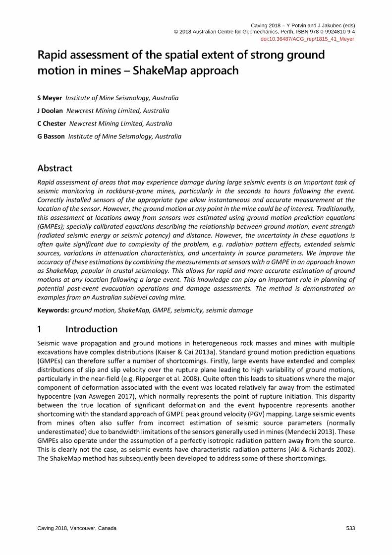
Two datasets are compiled. The first set, the calibration set, consists of all events recorded from 23 August 2016 to 30 October 2017 with LogP > -1.0 and located in the area of interest around the production levels. This dataset consists of 292 events (Figure 1).

Figure 1 Plan view (top) and east-facing section view (bottom) of the events used in the calibration

dataset. The majority of the LogP > -1.0 events are on the eastern flank, but the largest events

are on the western flank

Seismicity – tools to manage seismic risk


The observed ground motions of this set are compared to the estimated ground motions. Figure 2 shows the observed versus estimated plot, using the potency-based GMPE (Mendecki 2015) which was calibrated using 740 observations, with events ranging in size from LogP = 0.0 to LogP = 2.9, observation distances from 54 to 1,222 m and ground motions from 0.3 to 164 mm/s. This is used to estimate 𝜎𝑜𝑏𝑠, one of the parameters required for the ShakeMap method. The largest ground motions and largest outliers were manually checked. One event was excluded from this as it was inside a blasting sequence and the strongest ground motions were associated with the blast. Another event was excluded as it was a ‘double’ event, with two events inside the same waveform buffer. Only observations associated with the larger event and stronger ground motions were kept. Two events were found to have clipped waveforms with four observations in total, which were also excluded.

Figure 2 Observed versus predicted ground motions for events in the calibration dataset. Only ground

motions above 1 mm/s were considered. The largest outliers were manually examined and

removed if need be, e.g. due to electrical noise or multiple events in the waveform buffer

The second dataset represents the large events on which the method was tested. For this purpose, three of the largest events were selected. These are summarised in Table 1 and shown in Figure 3. The largest of these, LogP = 2.9 on 7 November 2014, is particularly large for a mining-induced seismic event (Malovichko & Meyer 2014). It is noted that all these events occurred following SLC production blasts, during post-blast seismic exclusion periods.

Table 1 Details of the target dataset, the large events on which the method was tested

# Date Time X (m) Y (m) Z (m) LogP LogE

1 07/11/14 06:12:30 60,394 11,575 4,499 2.9 8.2

2 16/11/16 06:42:48 60,494 11,066 4,416 1.4 6.9

3 24/07/17 06:08:20 60,462 10,932 4,463 1.5 7.0



Figure 3 Plan view (top) and east-facing section view (bottom) of the events used in the target dataset.

Purple triangles represent seismic sensors. Solid wireframes represent mined out stopes at

different time periods

3 Method

The method implemented here is based on the approach in Worden et al. (2010). The concept of the method is to combine observations at stations with a GMPE to improve estimates of ground motion at areas of interest. Measurements at sensors provide reliable and precise data points, but are very limited in space. GMPEs can provide estimates at any location of interest, but are much more uncertain than actual measurements. The ShakeMap approach aims to combine these two to deliver the most reliable results. For the GMPE, we use the potency-based GMPE from Mendecki (2015):

𝑃𝐺𝑉 = 5.02 × 𝑃0.68(5.25𝑃1 3⁄ + 𝑅)−1.49

(1)

where PGV is in m/s, P in m3 and R in m. This is the same equation used to generate the estimated PGV values in Figure 2.

The exact details of the ShakeMap implementation are not discussed here, but some key factors and concepts are introduced to explain and demonstrate the method, as illustrated in Figure 4.



Figure 4 Illustration of the method and associated geometry. Calculation of Yobs,x,i, the estimated ground

motion at point x inferred from observation point i. The equation for estimating σobs,x depends

on the value of rΔ. Point YA would use Equation 4 (observation dominates), YB Equation 5 (GMPE

dominates but observation plays a role), and YC would use Equation 6 (observation plays no role)

(adapted from Worden et al. 2010)

The first of these concepts is the estimated ground motion amplitude, 𝑌𝑜𝑏𝑠,𝑥 at a point �⃗�, based on nearby

observation, 𝑌𝑜𝑏𝑠:

𝑌𝑜𝑏𝑠,𝑥 = 𝑌𝑜𝑏𝑠 × (𝑌𝐺𝑀𝑃𝐸,�⃗⃗⃗�

𝑌𝐺𝑀𝑃𝐸,𝑜𝑏𝑠) (2)

where 𝑌𝐺𝑀𝑃𝐸,𝑥 and 𝑌𝐺𝑀𝑃𝐸,𝑜𝑏𝑠 are the estimated ground motions from the GMPE at point �⃗� and the

observation point (where the sensor is), respectively. The original work by Worden et al. (2010) also contains another adjustment for a local site effect. We exclude this aspect as we assume no site effects by considering all geophones and measurements are in boreholes. Equation 2 provides a single estimate based on a single measurement. This is now expanded to account for ground motion uncertainty and the contribution from multiple sites:

𝑌𝑥 = 𝑌𝐺𝑀𝑃𝐸,𝑥 ×

1

𝜎𝐺𝑀𝑃𝐸2 +∑ (

𝑌𝑜𝑏𝑠,�⃗⃗⃗�,𝑖𝑌𝐺𝑀𝑃𝐸,𝑜𝑏𝑠,𝑖

×1

𝜎𝑜𝑏𝑠,�⃗⃗⃗�,𝑖2 )𝑛

𝑖=1

1

𝜎𝐺𝑀𝑃𝐸2 +∑ (

1

𝜎𝑜𝑏𝑠,�⃗⃗⃗�,𝑖2 )𝑛

𝑖=1

(3)

where 𝜎𝐺𝑀𝑃𝐸 is the standard deviation of the GMPE. 𝜎𝑜𝑏𝑠,𝑥 is the standard deviation expected for a remote

estimation at point �⃗� based on an observation at sensor i and depends on the distance to the sensor. n is the total number of sensors used in the final approximation. In Mendecki (2015), a value of σGMPE = 0.355 was found for the dataset used to calibrate the GMPE. This estimated deviation is therefore based on some measurements that are perhaps not of interest to this task. This value is therefore re-evaluated using a more recent, independent dataset with a minimum threshold of 1 mm/s, and σGMPE = 0.363 was found, as shown in Figure 2.



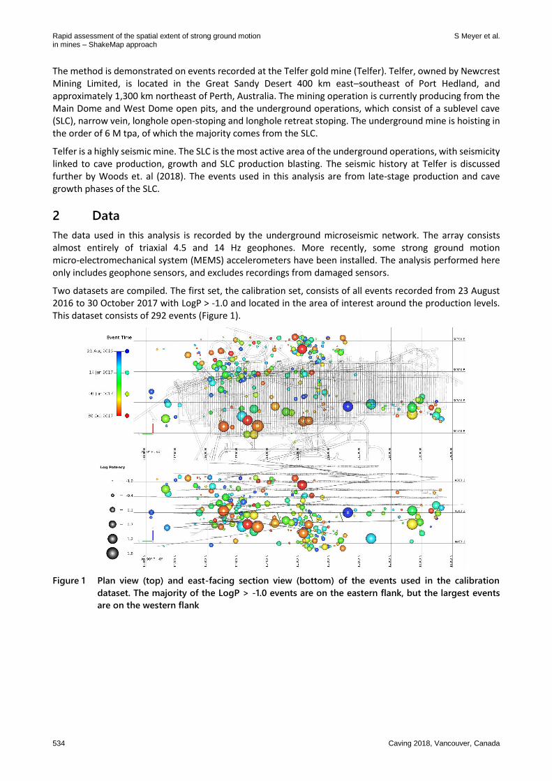
The value of σobs,x,i is a function of 𝑟𝛥, the distance between the estimation point �⃗� and the location of sensor i and can be based on one of the following three equations:

𝜎𝑜𝑏𝑠,𝑥 = 𝜎𝐺𝑀𝑃𝐸 . (1 − 𝑒𝑥𝑝(−√𝛼𝑟. 𝑟𝛥)) (4)

for 𝑟𝛥 ⩽ 𝑟𝑅𝑂𝐼,

𝜎𝑜𝑏𝑠,𝑥 = 𝜎𝑟=𝑟𝑅𝑂𝐼 .𝑟𝑚𝑎𝑥−𝑟𝑅𝑂𝐼

𝑟𝑚𝑎𝑥−𝑟𝛥 (5)

for 𝑟𝑅𝑂𝐼 < 𝑟𝛥 < 𝑟𝑀𝑎𝑥, and

𝜎𝑜𝑏𝑠,𝑥 = ∞ (6)

for 𝑟𝛥 > 𝑟𝑀𝑎𝑥

As discussed in Worden et al. (2010), rROI is an empirically estimated distance at which the observation’s standard deviation is equal to the GMPE’s. When r∆ is less than rROI , the contribution from the observation has more influence than the estimation from the GMPE. As r∆ approaches zero, i.e. interpolation point approaches an observation point, the observation dominates and the GMPE has negligible impact. In Worden et al. (2010), αr = 0.6 which is taken from Boore et al. (2003) who estimated this parameter for the California region, while rROI = 10 km and rmax = 15 km.

These values would clearly not be applicable for Telfer mine, which should have its own site-specific values estimated. To do this, we repeat the process from Boore et al. (2003) used to find αr:

For an event of interest, compute the interstation distance, ∆.

For each pair, compute the difference of the logarithm of the PGV after correcting for differences in distance from station to earthquake. The correction is calculated using the GMPE and its parameters, cl and cR, although cl has very minor impact unless R is very small:

𝑃𝐺𝑉𝐵 = 𝑃𝐺𝑉𝐴 [𝑐𝑙𝑃

1 3⁄ +𝑅𝐵

𝑐𝑙𝑃1 3⁄ +𝑅𝐴

]−𝑐𝑅

(7)

Divide the range of ∆ into bins so that there are 25 station pairs per bin. This value of 25 is arbitrary. Testing values between 10 and 30 yielded little variation.

Compute standard deviation of differences in each ∆ bin.

Plot these standard deviations against the median distances from each bin and fit a function.

This procedure was repeated for the events in the calibration dataset (Figure 1). As done in Boore et al. (2003) and Worden et al. (2010), we initially attempted fitting an exponential function. The fit from this was however not particularly good. We then repeated the process with a linear function. The fit of the linear function was only applied on ranges where σobs ≤ σGMPE . This also allowed us to estimate the point at which uncertainty in observations exceeds that of the GMPE, rROI , and was found to be about 265 m. Figure 5 illustrates these results and is effectively a reproduction of Figure A1 in Boore et al. (2003), done with recent Telfer data of interest.



Figure 5 Standard deviation of difference of log of PGV as a function of interstation distance. The red line

shows the fitted linear function up to a maximum distance of 265 m. The green curved line shows

the initial exponential fit

Following these results, we can estimate that for Telfer, Equation 4 should become:

𝜎𝑜𝑏𝑠,𝑥 = 𝜎𝐺𝑀𝑃𝐸 . (0.00139𝛥) (8)

where r∆ ≤ rROI and rROI = 265 m. Equation 5 simply acts as a tapering function and we keep the form the same as in Worden et al. (2010). For rmax, we choose 400 m. This selection is somewhat arbitrary, but has little impact on the results, and is similar to the value selected by Worden et al. (2010) when considered as a proportion of rROI .

4 Results

The method is applied to the events of interest listed in Table 1. The processing and overall waveform quality is checked to ensure that there are no spurious artefacts, e.g. electrical spikes.

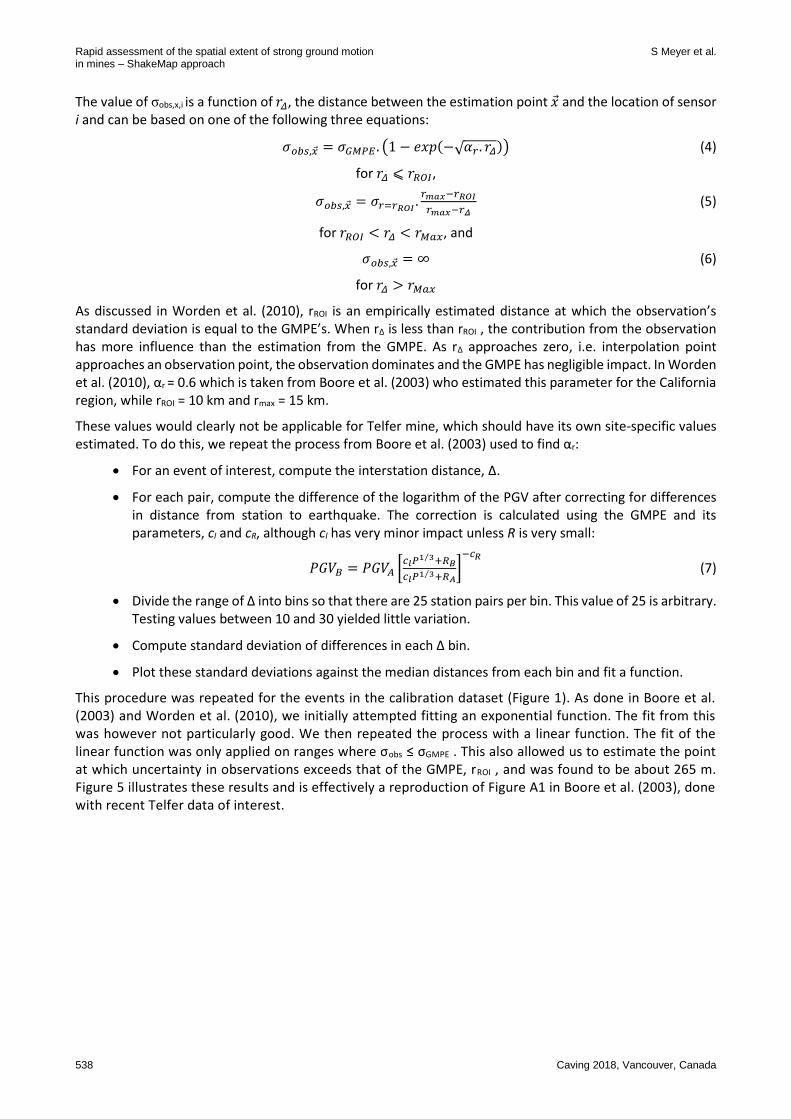
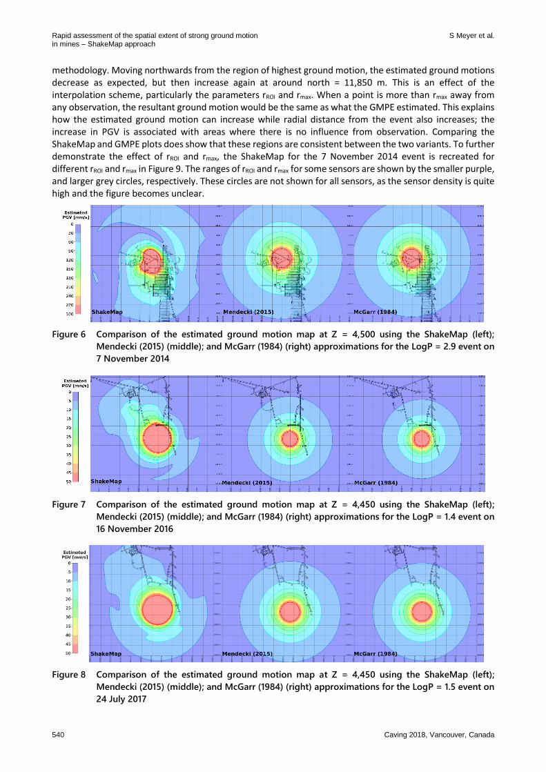
Figures 6 to 8 compare the results of the standard GMPE results and the ShakeMap for the different events in the target dataset using the calibrated values rROI = 265 m and rmax = 400 m. The GMPE plots use the LogP GMPE calibrated for Telfer mine (Mendecki 2015). The ShakeMap uses the equations listed in Equations 5, 6 and 8. For further comparison, we also compare the performance of the ShakeMap to the GMPE of McGarr (1984):

𝑃𝐺𝑉 = 10−4.78𝑀00.44𝑅−1 (9)

Assuming a rigidity of 𝜇 = 30𝐺𝑃𝑎, the potency-based version becomes:

𝑃𝐺𝑉 = 0.676 × 𝑃0.44𝑅−1 (10)

The most obvious feature of the plots is that the ShakeMap does not produce radially isotropic ground motions like the two GMPE methods. This is as expected, and highlights the exact purpose of the ShakeMap, leading to some cases where the ShakeMap estimate exceeds that of the GMPE while the opposite is true in other cases. For example, in Figure 6, the ShakeMap ground motion estimates are larger than those of the GMPE in areas to the south of the event, but less than the GMPE estimates to the west, north and east. The same figure also demonstrates another interesting, perhaps unexpected, behaviour in the ShakeMap



methodology. Moving northwards from the region of highest ground motion, the estimated ground motions decrease as expected, but then increase again at around north = 11,850 m. This is an effect of the interpolation scheme, particularly the parameters rROI and rmax. When a point is more than rmax away from any observation, the resultant ground motion would be the same as what the GMPE estimated. This explains how the estimated ground motion can increase while radial distance from the event also increases; the increase in PGV is associated with areas where there is no influence from observation. Comparing the ShakeMap and GMPE plots does show that these regions are consistent between the two variants. To further demonstrate the effect of rROI and rmax, the ShakeMap for the 7 November 2014 event is recreated for different rROI and rmax in Figure 9. The ranges of rROI and rmax for some sensors are shown by the smaller purple, and larger grey circles, respectively. These circles are not shown for all sensors, as the sensor density is quite high and the figure becomes unclear.

Figure 6 Comparison of the estimated ground motion map at Z = 4,500 using the ShakeMap (left);

Mendecki (2015) (middle); and McGarr (1984) (right) approximations for the LogP = 2.9 event on

7 November 2014



16 November 2016



24 July 2017



Figure 9 Results of the ShakeMap for the 7 November 2014 event for different rmax and rROI values;

rROI = 100 m and rmax = 150 m (left); rROI = 265 m and rmax = 400 m (middle); rROI = 600 m and

rmax = 1,000 m (right); at Z=4,500 m

Figure 10 compares the results of the ShakeMap with observed damage. The plot on the right compares the observed ground motions to the estimated ground motions according to the GMPE of Mendecki (2015). The waveforms at a number of nearby sensors are shown and are all clipped, leading to understated ground motion values. The data points within the red square were all associated with clipped measurements, and thus the true values would be higher and unknown.

Figure 10 The left plot shows the ShakeMap contours for the 7 November 2014 event. Purple regions

indicate areas of reported falls of ground (FOG) > 1 t (Newcrest Mining Limited 2014)

As is often observed following large seismic events in mines, damage can occur in localised and isolated patches. While strong ground motions can facilitate the occurrence damage, it is clearly not the sole decider. Local geological or design features can increase the local stress field, or ‘stress raisers’, leading to disparities of between observed damage and strong ground motion (Kaiser 2017). This illustrates the range of uncertainties of associated parameters and our lack of understanding of rockburst mechanism details (Dunn 2017).

5 Mine site application

An important aspect of this work for mine site applications is that the results can be accessed and viewed quickly and easily by geotechnical staff onsite. Figure 11 demonstrates how this could be implemented. Once the ShakeMap has been calibrated, seismic monitoring software is used to display the results on mine solids. This can be achieved by selecting the event, or otherwise the software can automatically estimate the ShakeMap for the largest, most recent event (e.g. within the last four hours).



Figure 11 Example of enabling the ShakeMap mine plans overlay in the 3D viewer. The results can be

displayed for the largest event in the currently visible time period, or for a user-selected event

This is useful, as following a large and potentially damaging seismic event, the site geotechnical engineer is required to investigate event source, mechanism, location and extent of rock mass damage and ground support condition. Also, depending on the location and potential severity of the event and mine protocols, a partial or whole mine evacuation may be required. A ShakeMap can facilitate initial investigations by providing a more reliable estimate of the spatial extent of strong ground motion, thus allowing geotechnical engineers to more rapidly evaluate the extent of potentially damaging ground motions and take appropriate action. Results are typically available as soon as the event is processed, normally within minutes of it occurring.

The ShakeMap results may also be used to compare measured (actual) versus forecast ground motions. Kaiser (2013b) describes that for forensic analysis of rockburst processes causing damage to underground excavations, the actual ground motion must be measured by field monitoring or predicted by synthetic ground motion models.

Although significant damage may not occur from an individual event, monitoring of the ShakeMaps over a period of time, say a month, allows the geotechnical engineer to isolate or focus additional monitoring and analysis on areas of the mine that have sustained repeated strong ground motions. Steps can then be taken to ensure appropriate mitigation controls are in place to address any ground support capacity consumption that may have occurred as a result of the cumulative effects of ground motion.

The calibrated and correlated ShakeMaps also form a powerful communication tool for the geotechnical engineer to effectively communicate both upwards and downwards to all levels of mine personnel due to the common understanding of heat maps. Presentation of seismic events as simple coloured spheres, scaled to magnitude, can lead to confusion and distraction from the message. Whereas ShakeMaps in the form of heat maps can communicate both spatial and risk (deformation potential) information as shown in Figure 11.



6 Discussion

The ShakeMap approach provides a relatively simple and efficient method of improving the estimates of strong ground motion from large seismic events by combining a GMPE with observations at sensors. GMPEs are known to be fairly uncertain due to complexities associated with large events, such as directivity, slip distribution and radiation pattern effects. By integrating the direct measurements from sensors, these complications are inherently accounted for. This does, however, highlight one of the potential drawbacks to the method, whereby corrupted measurements can skew the results. For example, clipping of sensors can lead to recorded ground motions being lower than what was really experienced. This is possible for both dynamic range clipping (sensor output voltage exceeding range of digitiser) or mechanical clipping (geophone mass physically reaching the maximum displacement limit). Although both of these situations would represent an underestimate of the ground motion, they would only occur in fairly extreme situations with very large events and strong ground motions, and would, therefore, not lead to a situation where potentially damaging ground motions were missed, just their exact values. Alternatively, false measurements of strong ground motions, such as electrical spikes, could potentially lead to estimates of strong ground motion that did not really occur.

The calibration of the ShakeMap, namely determining values for the parameters rROI and rmax, is also important. Figure 9 shows how changes to these parameters can influence the results. When these values are low, the results of the ShakeMap is much closer to that of the chosen GMPE. The ground motion map on the left of Figure 9 illustrates this. The contours of estimated ground motion are fairly concentric and very similar to that of the GMPE (middle plot of Figure 6), except for isolated patches showing variation. These patches are those areas within rmax of at least one sensor, as indicated by the circles. Conversely, setting rROI and rmax quite high (right plot of Figure 9) leads to the observations dominating and a much smoother set of contours. Setting rROI and rmax too low is clearly not useful, as it simply emulates the standard GMPE. Setting these values much higher might be considered desirable, but then the method also loses usefulness as the effects from all the observations begin to mix and smooth too much. These observations highlight that ShakeMap calibration should be completed by an experienced seismologist and occasionally be verified and updated if necessary, including when microseismic systems are expanded.

Regardless of the choice of rROI and rmax values, the best solution to maximise the benefit from the method is to ensure sufficient spatial coverage of reliable sensors, as illustrated in Figure 9. The three variants of the ShakeMap for this event are generally very different. However, in the nearby vicinity of sensors, the results are consistent. Even though the overall shape and form of the three different ShakeMaps vary quite significantly, they all have very similar ground motion values when very close to a sensor (centre of purple circles). Therefore, having many sensors at fairly constant sensor density would benefit the results significantly. Furthermore, for best results, the sensors and stations should have the ability to record strong ground motions without being corrupted due to clipping. Dynamic range clipping on geophones can be addressed, however, mechanical clipping cannot be avoided.

The 14 and 4.5 Hz geophones have peak-to-peak displacement limits of 0.5 and 4 mm, respectively. These values are insufficient to fully capture ground motion of large events when considering associated displacements, particularly when the sensors are located near the source. To avoid experiencing corrupted measurements, it is recommended that rockburst-prone mines install capable strong ground motion sensors, such as high-fidelity MEMS accelerometers. These sensors have the ability to record very strong ground motions without clipping. However, they are less sensitive to small ground motions and, therefore, the best approach is to utilise hybrid sensors that contain a triaxial MEMS accelerometer and triaxial 14 or 4.5 Hz geophone in the same sensor boat. The geophone is utilised for processing of small- and medium-sized events while the MEMS can be used to accurately retrieve the ground motions associated with less common, but more important, large events.

Figure 10 shows how clipped measurements can influence GMPE-based analyses. The site closest to the event hypocentre (ID 39) has estimated ground motion higher than observed, due to the close proximity to the event. The other sites that clipped, such as ID 47, all had estimated ground motions similar to, or lower than, the observed values. Therefore, if the observed values were not corrupted due to clipping, they would



have exceeded the estimated values. This would have led to even higher, and more accurate values of ShakeMap contours. Even though the measurement was underestimated due to clipping, as it exceeded the GMPE estimate, it still provided more reliable estimates of strong ground motions than the standard GMPE.

The main objective of this method and its application in mine seismology is to provide site-based geotechnical engineers with a way to quickly and reliably estimate and communicate which areas may have experienced strong, potentially damaging ground motion from a large seismic event, assisting with post-event seismic risk management and investigation protocols. While local geological and design features could dictate the exact locations of significant damage, identification of areas that experienced the strongest ground motions provides a guide as to where these may be. Future development of this method can look to incorporate such ‘stress raisers’ which may amplify the damage potential. Additionally, ShakeMaps in terms of cumulative absolute displacement (CAD) (Mendecki 2016) can provide insight into the longer term consumption of support capacity as it quantifies the cumulative deformation experienced at a location over time. CAD can provide a way to account for the effect of multiple smaller or medium-sized seismic events and their impact on support, while PGV is better suited for assessing potential damage associated with a single event.

Acknowledgement

The authors thank Newcrest Mining Limited for their collaboration and for permission to publish this work. Thanks also go to P Mountfort for providing valuable feedback regarding the clipped waveforms and to D Malovichko for discussing the calibration and interpretation of results.

References

Aki, K & Richards, PG 2002, Quantitative Seismology, University Science Books, Herndon. Boore, DM, Gibbs, JF, Joyner, WB, Tinsley, JC & Ponti, DJ 2003, ‘Estimated ground motion from the 1994 Northridge, California,

earthquake at the site of interstate 10 and La Cienega Boulevard bridge collapse, West Los Angeles, California’, Bulletin of the Seismological Society of America, vol. 93, no. 6, pp. 2737–2751.

Dunn, MJ 2017, ‘Dynamic ground support – design methodologies and uncertainties’, in J Wesseloo (ed), Proceedings of the Eighth International Conference on Deep and High Stress Mining, Australian Centre for Geomechanics, Perth, pp. 637–650.

Kaiser, PK & Cai, M 2013a, ‘Critical review of design principles for rock support in burst-prone ground – time to rethink!’, in Y Potvin & B Brady (eds), Proceedings of the Seventh International Symposium on Ground Support in Mining and Underground Construction, Australian Centre for Geomechanics, Perth, pp. 3–37.

Kaiser, PK & Cai, M 2013b, ‘Rockburst damage mechanisms and support design principles’, in A Malovhicko & D Malovhicko (eds), Proceedings of the Eighth International Symposium on Rockbursts and Seismicity in Mines, S RAS & MI UB RAS, Obninsk-Perm, pp. 349–370.

Kaiser, PK 2017, ‘Ground control in strainbursting ground – A critical review and path forward on design principles’, in J Vallejos (ed.), Proceedings of the Ninth International Symposium on Rockbursts and Seismicity in Mines, University of Chile, Santiago, pp. 146–158.

Malovichko, D & Meyer, S 2014, Telfer Mine: Analysis of the M2.9 Seismic Event on 7 Nov’14 and Related Seismicity, technical report, Institute of Mine Seismology, Hobart.

McGarr, A 1984, ‘Scaling of ground motion parameters, state of stress, and focal depth’, Journal of Geophysical Research: Solid Earth, vol. 89, no. B8, pp. 6969–6979.

Mendecki, AJ 2013, ‘Frequency range, log E, log P and magnitude’, in A Malovhicko & D Malovhicko (eds), Proceedings of the 8th International Symposium on Rockbursts and Seismicity in Mines, S RAS & MI UB RAS, Obninsk-Perm, pp. 167–173.

Mendecki, AJ 2015, Telfer Mine: Development of Ground Motion Prediction Equation for Telfer Mine Below 4650RL, technical report, Institute of Mine Seismology, Hobart.

Mendecki, AJ 2016, Mine Seismology Reference Book – Seismic Hazard, Institute of Mine Seismology, Hobart. Newcrest Mining Limited 2014, Seismic Event Investigation 2.7ML event 7-11-2014, Newcrest Internal Report: 700-200-GE-REP-1003,

Newcrest Mining Limited, Melbourne. Ripperger, J, Mai, PM & Ampuero, J-P 2008, ‘Variability of near-field ground motion from dynamic earthquake rupture simulations’,

Bulletin of the Seismological Society of America, vol. 98, no. 3, pp. 1207–1228. van Aswegen, G 2017, ‘Seismic sources and rockburst damage in South Africa and Chile’, in J Vallejos (ed.), Proceedings of the Ninth

International Symposium on Rockbursts and Seismicity in Mines, University of Chile, Santiago, pp. 72–86. Woods, MJ, Poulter, ME & King, RG 2018, ‘Progression and management of seismic hazard through the life of Telfer sublevel cave’,

in Y Potvin & J Jakubec (eds), Proceedings of the Fourth International Symposium on Block and Sublevel Caving, Australian Centre for Geomechanics, Perth, pp. 651–664.

Worden, CB, Wald, DJ, Allen, TI, Lin, K, Garcia, D, & Cua, G 2010, ‘A revised ground-motion and intensity interpolation scheme for ShakeMap’, Bulletin of the Seismological Society of America, vol. 100, no. 6, pp. 3083–3096.

rapid assessment of the spatial extent of strong ground

Documents