ORIGINAL PAPER

Rapid flood inundation mapping using social media,remote sensing and topographic data

J. F. Rosser1 • D. G. Leibovici1 • M. J. Jackson1

Received: 11 August 2016 /Accepted: 11 January 2017 / Published online: 25 January 2017� The Author(s) 2017. This article is published with open access at Springerlink.com

Abstract Flood events cause substantial damage to urban and rural areas. Monitoring water

extent during large-scale flooding is crucial in order to identify the area affected and to

evaluate damage. During such events, spatial assessments of floodwater may be derived from

satellite or airborne sensing platforms. Meanwhile, an increasing availability of smartphones

is leading to documentation of flood events directly by individuals, with information shared in

real-time using social media. Topographic data, which can be used to determine where

floodwater can accumulate, are now often available from national mapping or governmental

repositories. In this work, we present and evaluate a method for rapidly estimating flood

inundation extent based on a model that fuses remote sensing, social media and topographic

data sources. Using geotagged photographs sourced from social media, optical remote

sensing and high-resolution terrain mapping, we develop a Bayesian statistical model to

estimate the probability of flood inundation through weights-of-evidence analysis. Our

experiments were conducted using data collected during the 2014 UK flood event and focus

on the Oxford city and surrounding areas. Using the proposed technique, predictions of

inundation were evaluated against ground-truth flood extent. The results report on the

quantitative accuracy of the multisource mapping process, which obtained area under

receiver operating curve values of 0.95 and 0.93 for model fitting and testing, respectively.

Keywords Flood mapping � Data fusion � Data conflation � Data integration

1 Introduction

Flooding causes considerable damage to people, infrastructure and economies of many

countries of the world. During a flooding event, rapid estimation of inundated areas is

critical to effectively manage response operations. Emergency managers require timely and

& J. F. Rosserjulian.rosser@nottingham.ac.uk

1 Nottingham Geospatial Institute, University of Nottingham, Nottingham NG7 2TU, UK

123

Nat Hazards (2017) 87:103–120DOI 10.1007/s11069-017-2755-0

accurate information on areas affected by floodwater to prioritise relief efforts and plan

mitigation measures against damage.

Nowadays, large amounts of geospatial data can be derived from a multitude of sources.

In a time-critical disaster situation, utilisation of multiple data sources is particularly

desirable. Remote sensing from satellite and aircraft platforms can provide detailed

snapshots of a situation. However, these frequently do not provide the spatio-temporal

coverage required for flood assessment and may not be validated in the field. For example,

Landsat 8 provides multispectral data at 30-m spatial resolution, yet urban and semi-urban

environments can contain many features affecting floodwater movement and presence

within this cell size. Remote assessments can also have quality and uncertainty issues

resulting from the choice of processing algorithm, mixed spectral responses and back-

ground noise (Jiang et al. 2014).

Furthermore, the increasing proliferation of consumer devices, such as smartphones,

tablets and wearable logging sensors is facilitating the creation of large streams of data

(Goodchild 2007). However, despite much interest in using such sources in natural hazard

assessment (Goodchild and Glennon 2010), exploiting this information is not trivial. The

data usually have no validation or assessment of quality (Goodchild and Li 2012) and may

contain deliberate or unintended bias (Xiao et al. 2015).

To address these issues, we describe a method to integrate information derived from

multiple sources to aid in the estimation of flood inundation extent. Observations made by

in situ crowd users are combined with medium-scale optical remote sensing and a high-

resolution terrain model. Our main contribution is a probabilistic model, which quantita-

tively evaluates the contribution of each data source, and exploits contemporaneous remote

sensing, social media and high-resolution topographic models to estimate flood inundation

extent. Although our sample of social media is relatively small (n = 205), the importance

of this information can be quantified by our method and use this ranking within an overall

flood presence probability prediction. This enables even relatively small amounts of

crowdsourced information to add value to hazard assessments. Validation and assessment

of the proposed fusion-conflation model is undertaken demonstrating quantitative

improvements over mapping flood extent using a single data source.

2 Crowdsourcing and disaster assessment

In this section, we review approaches and research undertaken to exploit crowdsourced

data during natural disasters. We separate this work into two separate areas. Section 2.1

deals with citizen science type approaches where the ‘‘crowd’’ is actively engaged or

directed. Section 2.2 reviews studies using web-harvested geospatial data.

2.1 Volunteer-based assessment

The use of crowdsourced data has been explored in various papers and research pro-

grammes in relation to natural disaster assessment. Coordinated deployment of crowd

contributors is relatively well explored following earthquakes (Zook et al. 2010; Bar-

rington et al. 2011; Ghosh et al. 2011; Kerle and Hoffman 2013). These approaches

typically rely on citizen-based satellite or aerial image interpretation to assess disaster

damage. Crowdsourcing software platforms may also be used to assess ground-collected

images captured using smartphones. For example, the UNITAR-UNOSAT project

104 Nat Hazards (2017) 87:103–120

123

GeoTag-X aims at using volunteers to categorise images captured during disaster situations

and providing assessments, such as floodwater extent, damage to buildings or the safety of

temporary shelters for refugees (GeoTag-X 2015).

Poser and Dransch (2010) evaluated the use of volunteered geographic information for

flood damage assessment. The authors surveyed individuals affected by a river flooding

event to understand their perception of inundation and compared this to hydraulic mod-

elling predictions, identifying that non-professionals can make useful assessments of water

extent and depth.

Hung et al. (2016) describe the use of geo-referenced citizen reports in relation to flood

events. They describe a method to assess the credibility of the reports based on a proba-

bilistic model trained on a previous flood event. The model was then used to categorise

credibility on a subsequent event, highlighting that volunteered information may be

automatically ranked to enable more rapid and adoption within emergency management

contexts.

Le Coz et al. (2016) highlight the use of volunteer-based hydrological monitoring and

prediction. They describe the adoption of citizen-captured video footage to estimate

hydraulic data (e.g. water velocity and discharge) in flash flooding situations. Furthermore,

the authors describe development and deployment of an interpolation approach using

citizen’s photographs of maximum flood levels in conjunction with LiDAR surface

models, and supplementary field assessment by professionals, in order to generate water

depth maps.

In our work, we choose to investigate use of social media data as that follows events in

real time, enabling capture of unpredictable situations and with the potential of a large

sample of well-positioned data. For these reasons, we focus the remaining review of the

literature on this topic.

2.2 Social media

Using information from social media for aiding decision-making is a problematic task.

This is due to multiple reasons including the challenge of extracting relevant information

(e.g. identifying topicality) within unstructured or semi-structured web-harvested data,

unknown quality (there may be little or no relevant metadata), and difficulty integrating it

with other sources (which may in turn have their own issues of quality and uncertainty).

When using social media, biases may also be present, for example, from a lack of digital

engagement within certain demographics of the populations of particular areas (Xiao et al.

2015).

Panteras et al. (2014) cross-reference geotagged points of images mined from Flickr and

tweets to estimate spatial footprints events. The authors extract toponyms expressed in

tweets to aid in estimating the viewing direction of Flickr images depicting a wildfire

event, leading to a more accurate delineation of the event. However, the authors do not

utilise remotely sensed earth observation data within their methodology, which is often

available in disaster situations.

Several research projects have analysed social media specifically during flood disasters.

Albuquerque et al. (2015) provide an example of the use of social media during flood

events. They built a statistical model of tweets as they relate to authoritative river levels. In

particular, the model tested the association between tweet locations and the water level in

flood-affected catchments.

Schnebele et al. (2014b) describe an interpolation-based approach that incorporates non-

authoritative data such as geotagged airborne (oblique) photographs and terrestrial videos

Nat Hazards (2017) 87:103–120 105

123

to provide a spatio-temporal flood damage assessment. Furthermore, integrating social

media data with remote sensing, river gauge measurements and digital elevation models

(DEM) has been shown to be effective at producing near-real-time flood hazard maps

(Schnebele and Cervone 2013). Fusion-based approaches can also aid extent estimation

when the data sources have incomplete coverage (Schnebele et al. 2014a). However, these

approaches rely on subjective user determination of weights for the model variables.

3 Study area

From December 2013 to February 2014, many parts of the UK were affected by flooding.

These events resulted from a series of major storms generating intense rainfall, severe

coastal gales and exceptional river flow rates (Slingo et al. 2014). Furthermore, a lack of

investment in river dredging, flood defence schemes, intensive agricultural practice and

inappropriate development of floodplains are thought to have exacerbated levels of

flooding (Thorne 2014). The impact of the inundation was sufficient to invoke activation of

the International Charter (International Charter 2000), a mechanism for making satellite

data available for disaster response, on 4/12/13, 6/1/14 and 6/2/14.

The study area is centred on the city of Oxford, shown in Fig. 1. The area encompasses

154.35 km2. Multiple watercourses flow through and converge in the city and its sur-

roundings. The Thames (Isis) and Cherwell form the major river systems with many

smaller streams and brooks as tributaries. The landscape is predominantly made up of

urban and agricultural uses with small tracts of mixed forest cover. Oxford city is thought

to be primarily at risk of fluvial flood events (OCC 2011). Groundwater flooding is also

known to be a risk factor (OCC 2011; Macdonald et al. 2012). In the city, 4500 properties

Fig. 1 Study area location within Great Britain, ground-truth flood extent, training and testing points

106 Nat Hazards (2017) 87:103–120

123

are thought to be at risk of flooding, rising to 6000 properties by 2080 as a result of the

effects of climate change (Envrionment Agency 2015).

4 Methodology

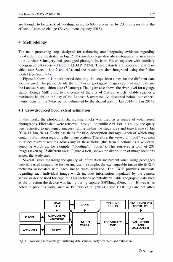
The main processing steps designed for estimating and integrating evidence regarding

flood extent are illustrated in Fig. 2. The methodology describes integration of near-real-

time Landsat 8 imagery and geotagged photographs from Flickr, together with ancillary

topographic data (derived from a LIDAR DTM). These datasets are processed and clas-

sified (see Sects. 4.1, 4.2 and 4.3), and the results are then integrated using the fusion

model (see Sect. 4.4).

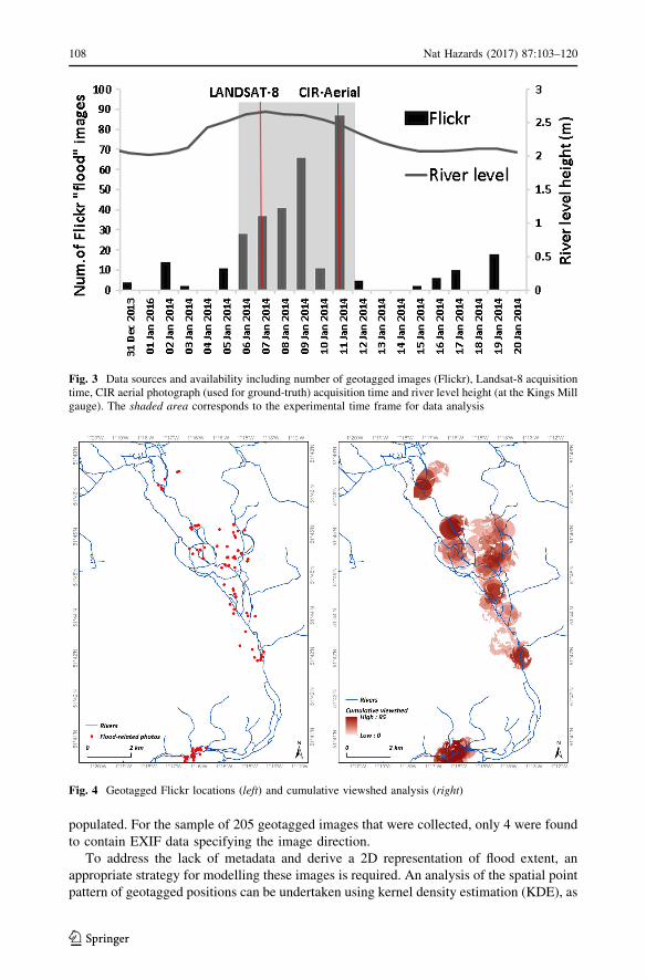
Figure 3 shows a 1-month period detailing the acquisition times for the different data

sources used. The period details the number of geotagged images captured each day and

the Landsat 8 acquisition date (7 January). The figure also shows the river level for a gauge

station (Kings Mill) close to the centre of the city of Oxford, which notably reaches a

maximum height on the day of the Landsat 8 overpass. As discussed below, our experi-

ments focus on the 7-day period delineated by the shaded area (5 Jan 2014–11 Jan 2014).

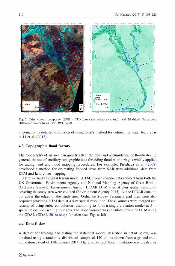
4.1 Crowdsourced flood extent estimation

In this work, the photograph-sharing site Flickr was used as a source of volunteered

photographs. Flickr data were retrieved through the public API. For this study, the query

was restricted to geotagged imagery falling within the study area and time frame (5 Jan

2014–11 Jan 2014). Flickr has fields for title, description and tags—each of which may

contain information regarding the image content. Therefore, the keyword ‘‘flood’’ was used

to detect relevant records across any of these fields (this term functions as a wildcard,

detecting words as, for example, ‘‘flooding’’, ‘‘floods’’). This retrieved a total of 205

images taken by 25 different users. Figure 4 (left) shows the distribution of image locations

across the study area.

Several issues regarding the quality of information are present when using geotagged

web-harvested images. To further analyse the sample, the exchangeable image file (EXIF)

metadata associated with each image were retrieved. The EXIF provides metadata

regarding each individual image which includes information populated by the camera

sensor or device used for capture. This includes potentially valuable geographic data such

as the direction the device was facing during capture (GPSImageDirection). However, as

noted in previous work, such as Panteras et al. (2014), these EXIF tags are not often

Fig. 2 Processing methodology illustrating data sources, analytical steps and validation

Nat Hazards (2017) 87:103–120 107

123

populated. For the sample of 205 geotagged images that were collected, only 4 were found

to contain EXIF data specifying the image direction.

To address the lack of metadata and derive a 2D representation of flood extent, an

appropriate strategy for modelling these images is required. An analysis of the spatial point

pattern of geotagged positions can be undertaken using kernel density estimation (KDE), as

Fig. 3 Data sources and availability including number of geotagged images (Flickr), Landsat-8 acquisitiontime, CIR aerial photograph (used for ground-truth) acquisition time and river level height (at the Kings Millgauge). The shaded area corresponds to the experimental time frame for data analysis

Fig. 4 Geotagged Flickr locations (left) and cumulative viewshed analysis (right)

108 Nat Hazards (2017) 87:103–120

123

adopted in Schnebele and Cervone (2013). These unsupervised methods learn a proba-

bilistic surface based on the 2D point pattern. Rather than use a kernel-based method, we

take a similar approach to Panteras et al. (2014) and adopt a viewshed-based model.

Specifically, the cumulative viewshed is used, first adopted for archaeological analysis

(Wheatley 1995). Here a viewshed for each photograph is calculated with each pixel

labelled as visible (value = 1) or not visible (value = 0). A summation over all viewsheds

therefore gives the number of times a location is visible from any photograph. This avoids

the necessity of selecting a bandwidth parameter, as required by kernel density estimation,

and takes account of topography—an important consideration in flood scenarios. The

viewshed methodology provides a measure of corroboration between individual geotagged

photographs at the pixel level and thus provides a model of agreement on where possible

flooded areas may be. The viewshed methodology implemented here assumes a viewer

height of 1.6 m, 360� viewing angle and a maximum viewing distance of 500 m. Although

the focal length of the camera image might be utilised, this information was not present in

the EXIF data. Thus, we chose a maximum viewing distance of 500 m based upon the

range that would be effectively observable (e.g. a photograph taken at edge of a flooded

field could extend to this range). The LIDAR DTM (described in further detail below) is

used by viewshed algorithm for defining topography. The result of the cumulative view-

shed analysis is shown in Fig. 4 (right).

4.2 Landsat 8 water detection

Both multispectral and SAR satellite remote sensing is commonly used for assessing

inundation extent during flood events. The operational land imager (OLI) instrument of

Landsat 8 provides multispectral data at 30-m spatial resolution. A single Landsat 8-OLI

image was obtained from the US Geological Survey (USGS) Global Visualization Viewer

as Level 1 Terrain Correct (L1T) product. One scene acquired on 7th January 2014 (path/

row: 203, 24) was obtained with cloud-free coverage of the study area. A small section in

the south-eastern corner of the study area fell outside the acquisition swath and thus is

missing data. Digital number (DN) values for the scene were converted to surface

reflectance (see Fig. 5, left) using the dark object subtraction (DOS) method (Chavez Jr

1996) available in QGIS. Further data pre-processing steps undertaken here involved

stacking Landsat bands 1–7 (30 m), re-projecting to British National Grid, cropping to the

study area undertaken using GDAL.

One frequently applied approach for detecting water given spectral response at

appropriate infrared wavelengths is to compute the Normalised Difference Water Index

(NDWI) (McFeeters 1996). However, using the Modified NDWI (MNDWI) has the

advantage of suppressing the response of both vegetation and built-up areas leading to

enhanced water detection for these areas (Xu 2006). This is applicable to the landscape

found in the Oxford study area and as such, we adopt this method here (see Fig. 5, right).

MNDWI can be expressed as:

MNDWI ¼ Green�MIR

GreenþMIRð1Þ

where MIR corresponds to band 7 (SWIR2, 2.11–2.29 l) of the L8-OLI instrument. As an

index method, a threshold for discriminating between water and non-water areas is

required. The threshold value for identifying areas of water can be assessed by expert or

automatically determined using methods such as Otsu’s algorithm (Otsu 1979). The

method uses the maximum between-class variance to determine the threshold. For further

Nat Hazards (2017) 87:103–120 109

123

information, a detailed discussion of using Otsu’s method for delineating water features is

in Li et al. (2013).

4.3 Topographic flood factors

The topography of an area can greatly affect the flow and accumulation of floodwater. In

general, the use of ancillary topographic data for aiding flood monitoring is widely applied

for aiding land and flood mapping procedures. For example, Pierdicca et al. (2008)

developed a method for estimating flooded areas from SAR with additional data from

DEM and land cover mapping.

Here we build a digital terrain model (DTM) from elevation data sourced from both the

UK Government Environment Agency and National Mapping Agency of Great Britain

(Ordnance Survey). Environment Agency LIDAR DTM tiles at 2-m spatial resolution

covering the study area were collated (Environment Agency 2015). As the LIDAR data did

not cover the edges of the study area, Ordnance Survey Terrain 5 grid tiles were also

acquired providing DTM data at a 5-m spatial resolution. These sources were merged and

resampled using cubic convolution resampling to form a single elevation model at 5-m

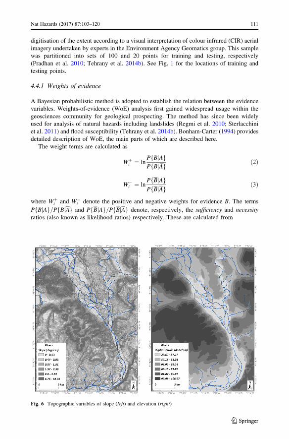
spatial resolution (see Fig. 6, right). The slope variable was calculated from the DTM using

the GDAL (GDAL 2016) slope function (see Fig. 6, left).

4.4 Data fusion

A dataset for training and testing the statistical model, described in detail below, was

obtained using a randomly distributed sample of 120 points drawn from a ground-truth

inundation extent of 11th January 2014. The ground-truth flood inundation was created by

Fig. 5 False colour composite (RGB = 632) Landsat-8 reflectance (left) and Modified NormalisedDifference Water Index (MNDWI, right)

110 Nat Hazards (2017) 87:103–120

123

digitisation of the extent according to a visual interpretation of colour infrared (CIR) aerial

imagery undertaken by experts in the Environment Agency Geomatics group. This sample

was partitioned into sets of 100 and 20 points for training and testing, respectively

(Pradhan et al. 2010; Tehrany et al. 2014b). See Fig. 1 for the locations of training and

testing points.

4.4.1 Weights of evidence

A Bayesian probabilistic method is adopted to establish the relation between the evidence

variables. Weights-of-evidence (WoE) analysis first gained widespread usage within the

geosciences community for geological prospecting. The method has since been widely

used for analysis of natural hazards including landslides (Regmi et al. 2010; Sterlacchini

et al. 2011) and flood susceptibility (Tehrany et al. 2014b). Bonham-Carter (1994) provides

detailed description of WoE, the main parts of which are described here.

The weight terms are calculated as

Wþi ¼ ln

PfBjAgPfBj�Ag ð2Þ

W�i ¼ ln

PfBjAgPfBjAg

ð3Þ

where Wþi and W�

i denote the positive and negative weights for evidence B. The terms

PfBjAg=PfBjAg and PfBjAg=PfBjAg denote, respectively, the sufficiency and necessity

ratios (also known as likelihood ratios) respectively. These are calculated from

Fig. 6 Topographic variables of slope (left) and elevation (right)

Nat Hazards (2017) 87:103–120 111

123

PfBjAg ¼ NfB \ AgNfAg ð4Þ

PfBjAg ¼ NfB \ AgNfAg

ð5Þ

PfBjAg ¼ NfB \ AgNfAg ð6Þ

PfBjAg ¼ NfB \ AgNfAg

ð7Þ

where A denotes the area of known occurrences of the phenomena based on the training

sample, B denotes the area of an evidence variable, and N{} denotes the count of the grid

cells. Intuitively, within this work, these equations calculate proportions for the presence

and absence of flood given presence and absence of the binary evidence.

In WoE, continuous variables must be discretised to form multiclass evidence data.

Once weights for the evidence data have been calculated, the maps may be integrated

together. The standard approach to applying WoE is to then convert multiclass evidence to

binary evidence variables. While an index of susceptibility can be calculated based on a

summation of contrast C (Oh and Lee 2010; Regmi et al. 2010), a map of posterior

probability may be calculated through identification of the appropriate cut-off value

determined from an analysis of contrast C (Bonham-Carter 1994). The ratio of the contrast

to standard deviation, C/s(C), provides a statistical test for determination of the optimal

cut-off point for each variable. Specifically, the threshold can be determined as the point

where C/s(C) is greater than or equal to a defined confidence level. The two final weights

for this binary map are assigned from the W? and W- values at this threshold point.

Assuming conditional independence between evidence variables (i.e. P(B1B2|-

A) = P(B1|A)P(B2|A)), logarithmic posterior probability maps may be computed using

L ¼ logitfAjB1 \ B2 \ B3 \ � � �Bng ¼ logitfAg þXn

i¼1

Wi ð8Þ

where logit{A} denotes the prior logarithmic odds of a flooded location given its prior

probability P(A). Therefore

logitfAg ¼ logðPðAÞ=1� PðAÞÞ ð9Þ

The prior probability p(A) can be calculated as the proportion of known flood locations to

the study area.

PðBÞ ¼ NfAg=NfTg ð10Þ

where N{T} is the total area.

Weight Wi corresponds to either Wþi or W�

i based on the presence or absence of the

evidence, respectively. Then converting to a probability

Pflood ¼expðLÞ

ð1þ expðLÞÞ ð11Þ

where Pflood is the probability of a flooded location.

112 Nat Hazards (2017) 87:103–120

123

Computing posterior probability maps using weights of evidence requires an assumption

of conditional independence between evidence variables. In geospatial problems, this

assumption may be violated to some degree as spatial data can often exhibit correlations

and therefore examination of the conditional independence should be undertaken (Bon-

ham-Carter 1994; Agterberg and Cheng 2002)

For discretisation in this work, a six-class quantile reclassification scheme was applied

to variables with continuous values, i.e. Flickr cumulative viewshed, slope and elevation

variables. Quantile classification was chosen due to its previous application to hazard

mapping using evidence variables (Dickson et al. 2006; Tehrany et al. 2014b). As binary

evidence, the MNDWI variable does not require reclassification.

5 Results

In this section, we present experimental results of applying the proposed workflow for

estimating flood extent. First, we analyse the calculated weight and contrast values which

quantify positive and negative correlations with flooded locations provided by each indi-

vidual data source (Sect. 5.1). Secondly, evaluation of the predictive power of the indi-

vidual data sources and their integration together as a posterior probability model is made

against ground-truth flood extent data (Sect. 5.2). Thirdly, we generate a flood extent map

based on the posterior probability (Sect. 5.3).

5.1 Evidence weights

Table 1 details the weight calculations (W?, W-) for each evidence variable class. Fig-

ure 7 plots the weight contrast (C) for each of the multiclass data sources. Recall from

Sect. 4.4.1 that the contrast can be used to help assess the importance of each class and

determine a binary cut-off threshold for the influence of a variable.

As described in Sect. 4.4.1, the cumulative viewshed Flickr extent was classified using

quantiles (Viewshed-01 to Viewshed-06). In Table 1 and Fig. 7 (left), the influence (W?)

and weight contrast (C) of the viewshed extent remain negative for the first three classes

(Viewshed-01 to Viewshed-03), with a strong positive correlation for classes 4–6

(Viewshed-04 to Viewshed-06). This corresponds to what we would expect given an

overestimation of flooded extent provided by the viewshed methodology described in

Sect. 4.1. However, classes 4–6 relate to areas where the viewshed extent is corroborated

by multiple images, correlating with flooded locations and lead to an increased positive

weight (weight values of 1.72, 1.60, and 1.54).

Notably, the weight values for the Flickr cumulative viewshed are close to that found in

Landsat-8 MNDWI water detection class, which has a strong positive weight (W?) of 2.11.

Recall from Sect. 4.2 that the water detection is based on a binary threshold derived using

the Otsu method, a commonly used method for detecting flood presence. Given this, we

can expect this detection to be influential in detecting flood presence.

The results also demonstrate correlations of topographic evidence variables with flood

locations. As seen in Table 1, lower elevations exhibited a high positive correlation with

flood locations, ranging from 1.42 to 0 for positive weight values (W?). The positive

weight value for the slope variable is seen to provide a slightly weaker correlation ranging

from 0.63 to 0.0 for gentle to steep slopes respectively. As discussed in Sect. 4, analysis of

the contrast (C) and C/s(C) values enables determination of an appropriate cut-off to

Nat Hazards (2017) 87:103–120 113

123

determine the final evidence variable class weight (visual assessment of Fig. 7 (centre) and

Fig. 7 (right) does not show a clear distinction for this cut-off). Here, a value of 2 is chosen

for the confidence level (Bonham-Carter 1994). This calculation forms a Studentised

measure of the certainty with which the contrast is known—i.e. a large value indicates an

effect that is more likely to be real. Slope values covering values of 0�–0.86� and elevation

covering altitudes of 28.63–58.81 m defined this threshold, and the final evidence weight

Wfin, shown in Table 1.

Table 1 Results of initial weight calculation (W?,W2), contrast (C), standard deviation of contrast (s(C)),studentised contrast (C/s(C)), final weight selected (Wfin) and its standard deviation (s(Wfin)) for evidencelayers

Evidence variable class Number ofcells

W? W- C s(C) C/s(C) Wfin s(Wfin)

Flickr cumulative viewshed

Viewshed01 5,598,238 -0.23 1.10 -1.33 0.22 -5.97 -0.23 0.12

Viewshed02 160,302 -0.26 0.01 -0.27 0.71 -0.37 -0.15 0.50

Viewshed03 126,383 -0.02 0.00 -0.02 0.71 -0.03 -0.15 0.50

Viewshed04 110,037 1.72 -0.09 1.81 0.33 5.44 1.72 0.32

Viewshed05 99,895 1.60 -0.07 1.67 0.37 4.52 1.60 0.35

Viewshed06 79,145 1.54 -0.05 1.59 0.42 3.78 1.54 0.41

Lansat-8 Modified Normalised Difference Water Index

MNDWI Non-water 5,306,975 -1.57 2.11 -3.68 -14.08 -14.08 -1.57 0.24

MNDWI Water 579,843 2.11 -1.57 3.68 14.08 14.08 2.11 0.11

MNDWI (MD) 287,182 0.00 0.00 0.00 0.00 0.00 0.00 0.00

Topographic data—slope

Slope 0�–0.43� 2,331,865 0.63 -0.76 1.39 0.22 6.33 0.37 0.10

Slope 0.44�–0.86� 3,887,775 0.37 -1.41 1.78 0.35 5.10 0.37 0.10

Slope 0.87�–1.51� 4,646,052 0.21 -1.26 1.47 0.39 3.76 -1.41 0.33

Slope 1.52�–2.59� 5,414,922 0.10 -1.41 1.51 0.59 2.58 -1.41 0.33

Slope 2.6�–4.74� 5,902,486 0.03 -1.48 1.52 1.01 1.51 -1.41 0.33

Slope 4.75�–54.95� 6,174,000 0.00 11.03 -11.03 14.14 -0.78 -1.41 0.33

Topographic data—elevation

Elevation28.63–56.07 m

1,226,214 1.42 -1.49 2.91 0.22 11.19 1.00 0.10

Elevation56.08–58.81 m

2,252,396 1.00 -4.15 5.15 5.12 5.12 1.00 0.10

Elevation58.82–63.75 m

3,317,417 0.62 -8.44 9.06 0.91 0.91 -4.15 1.00

Elevation63.76–73.63 m

4,288,052 0.36 -8.02 8.39 0.84 0.84 -4.15 1.00

Elevation73.64–92.84 m

5,267,575 0.16 -7.29 7.45 0.75 0.75 -4.15 1.00

Elevation92.85–168.57 m

6,174,000 0.00 11.03 -11.03 -0.78 -0.78 -4.15 1.00

M.D missing data

114 Nat Hazards (2017) 87:103–120

123

5.2 Model testing and validation

Receiver operating characteristic (ROC) and area under curve ROC (AUROC) analysis

was used to assess the performance of the individual data sources derived from Landsat-8

MNDWI and Flickr analysis, and the posterior probability model generated from com-

bining all sources using weights of evidence. In brief, ROC assessments are typically used

to measure the predictive power of a model to detect a binary outcome and are often used

for validating susceptibility models and mapping tasks (such as Devkota et al. (2013) and

Tehrany et al. (2014a)). The ROC curve plots the false positive rate (1-specificity) against

the true positive rate (sensitivity). The sensitivity and specificity provide an evaluation of

the model at correctly identifying flooded locations (true positive rate) and non-flooded

locations (true negative rate).

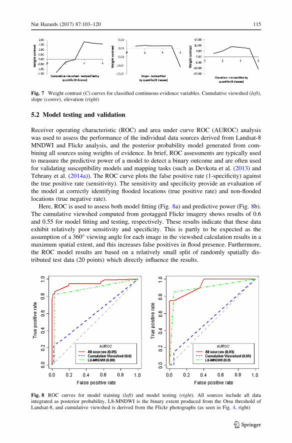
Here, ROC is used to assess both model fitting (Fig. 8a) and predictive power (Fig. 8b).

The cumulative viewshed computed from geotagged Flickr imagery shows results of 0.6

and 0.55 for model fitting and testing, respectively. These results indicate that these data

exhibit relatively poor sensitivity and specificity. This is partly to be expected as the

assumption of a 360� viewing angle for each image in the viewshed calculation results in a

maximum spatial extent, and this increases false positives in flood presence. Furthermore,

the ROC model results are based on a relatively small split of randomly spatially dis-

tributed test data (20 points) which directly influence the results.

Fig. 7 Weight contrast (C) curves for classified continuous evidence variables. Cumulative viewshed (left),slope (centre), elevation (right)

Fig. 8 ROC curves for model training (left) and model testing (right). All sources include all dataintegrated as posterior probability, L8-MNDWI is the binary extent produced from the Otsu threshold ofLandsat-8, and cumulative viewshed is derived from the Flickr photographs (as seen in Fig. 4, right)

Nat Hazards (2017) 87:103–120 115

123

ROC analysis of the Landsat-8 MNDWI binary flood mapping based on the Otsu

threshold was also completed. This identified a model fitting error of 0.88 and testing error

of 0.90 indicating that this data source is very effective at delineating flooded areas.

Generation of the all sources (L8-MNDWI, Flickr cumulative viewshed and topo-

graphic variables) flood model was undertaken through calculation of posterior of prob-

ability, as specified by Eqs. 8–11. The validation of the posterior probability map shows

AUROC values of 0.95 and 0.93 for model fitting and testing, respectively.

Testing of the resulting probability map incorporating all data sources was carried out

indicating no significant violations of conditional independence. A conditional indepen-

dence ratio of 6.38 was calculated, well above the recommended upper threshold of 1

suggested by Bonham-Carter (1994).

5.3 Flood extent map generation

Using a cut-off point determined from the ROC analysis of the training data, binary flood

extent maps may be generated from the probabilistic flood map. The cut-off point that

equally maximised both sensitivity and specificity was chosen using the ROCR package

(Sing et al. 2005). Figure 9 (right) shows the binary extent flood map against the CIR

ground-truth extent.

6 Discussion

The results demonstrate that incorporation of multiple sources of data can aid prediction of

flood extents using the proposed methodology. Despite this, several important assumptions

must be noted. Firstly, this work does not consider temporal aspects of the data within the

Fig. 9 Flood extent maps based on posterior probability (left) and probability cut-off calculated using ROCanalysis

116 Nat Hazards (2017) 87:103–120

123

modelling process as this case study involved a prolonged flooding event. Consideration of

the temporal aspects would be important for generalising the work to flash flood mapping

scenarios. Secondly, one drawback of the weights-of-evidence approach is the need for

variable discretisation. This can result in information loss if sufficient consideration is not

given to the modelling problem and evidence data used. This means that the proposed

methodology cannot be applied in a completely automated fashion unless an automatic

choice of number of classes is performed.

The work described here exploited a data-driven fusion model to integrate variables

which inform the desired analytical output—in this case a map of flood extent. However, in

other disaster scenarios alternative outputs might be more valuable. For example, identi-

fication of the areas where there is high uncertainty might be useful, allowing for further

remote interrogation or field investigation. The weights-of-evidence approach supports this

through enabling analysis of the weight variance (Dickson et al. 2006). Extension of the

analysis of either the weights or uncertainty with ensemble learning methods also offers the

potential of improving the results.

Although the experiments here exploit geotagged images sourced from social media, the

rapid inundation mapping methodology employed could incorporate other crowdsourced

assessments such as Twitter (Panteras et al. 2014; Smith et al. 2015) or volunteered by

citizens (Poser et al. 2009). Similarly, other authoritative data sources may be relevant

depending on the context. Within the UK, for example, many large watercourses are

gauged. Where this is the case, both river flow measurements and river level data are

usually available and this might be incorporated through linear interpolation of depth levels

as an indication of maximal water extent (Apel et al. 2009) or inclusion of an appropriate

2D hydrological inundation model (Liu et al. 2015). Other remote sensing platforms may

also be utilised as independent sources of evidence, such as SAR (Mason et al. 2010;

Matgen et al. 2011; Schumann et al. 2013).

Data quality is often discussed in relation to use of crowdsourced information. In terms

of rapid inundation mapping, the data sources expose different levels of uncertainty. On

one side with authoritative data, this uncertainty comes from a controlled quality assurance

but which needs to be modified due to the assessment time difference. On the other side,

various crowdsourcing data (e.g. Flickr, citizen science, Twitter) come with less controlled

quality assurance, but are timely. This reflects a recognised issue in the use of volunteered

data for natural hazard assessment where data quality is a concern, but its adoption is

particularly desirable (Goodchild and Glennon 2010; Haworth 2016). Our work evaluated a

sample of social media data taken for a large and serious flooding event retrieved via

keyword search. Despite this, the small size of the retrieved social media, and relatively

poor performance of this information when used on its own, highlights that crowdsourced

data currently must be used in combination with traditional flood mapping methods.

However, novel additional techniques for identifying relevant social media reports and

increasing samples sizes of digital reporting from citizens may relax this requirement (as

long as its quality can be assured). The fusion method proposed did not take into account

the quality of the information, but the workflow proposed here could integrate a quality

assurance step (e.g. such as a probabilistic credibility assessment (Hung et al. 2016)), even

if the algorithms used in quality assurance and in data fusion present some entanglement

(Leibovici et al. 2015).

Nat Hazards (2017) 87:103–120 117

123

7 Conclusions

This paper presented the methodology and experimental results of a rapid flood mapping

workflow using social media, remote sensing and topographic map data. Using a Bayesian

statistical model based on weights-of-evidence analysis, a data-driven approach was

developed which quantifies the contribution of each information source. Combining these

sources together enables generation of a probability map denoting likelihood of the

presence of floodwater at the pixel level. A case study using data relating to the 2014 UK

flood event was completed. ROC assessment and AUROC values demonstrated that the

multisource flood mapping method effectively predicts spatial extent of water. Further-

more, the methodology shows that even relatively simple voting-based procedures for

controlling for the quality of non-authoritative social media data may be integrated in a

flood assessment workflow. In future work, we will investigate the effects of uncertainty

within the data, such as positional accuracy of the geotagged photographs and the

imprecision of viewing direction, on the predicted flood extent.

Acknowledgements This work was supported by the Advanced Geospatial Information and IntelligenceServices (AGIS) project (UK MOD Contract No: DSTLX-1000063699) and the Citizen Observatory WEB(COBWEB) project funded by the European Union under the FP7 ENV.2012.6.5-1 funding scheme, EUGrant Agreement Number: 308513. The authors thank the UK Environment Agency Geomatics team forsupplying the ground-truth data for this study.

Open Access This article is distributed under the terms of the Creative Commons Attribution 4.0 Inter-national License (http://creativecommons.org/licenses/by/4.0/), which permits unrestricted use, distribution,and reproduction in any medium, provided you give appropriate credit to the original author(s) and thesource, provide a link to the Creative Commons license, and indicate if changes were made.

References

Agterberg F, Cheng Q (2002) Conditional independence test for weights-of-evidence modeling. Nat ResourRes 11:3–9. doi:10.1023/A:1021193827501

Albuquerque JP, Herfort B, Brenning A, Zipf A (2015) A geographic approach for combining social mediaand authoritative data towards identifying useful information for disaster management. Int J Geogr InfSci. doi:10.1080/13658816.2014.996567

Apel H, Aronica GT, Kreibich H, Thieken AH (2009) Flood risk analyses—how detailed do we need to be?Nat Hazards 49:79–98. doi:10.1007/s11069-008-9277-8

Barrington L, Ghosh S, Greene M et al (2011) Crowdsourcing earthquake damage assessment using remotesensing imagery. Ann Geophys. doi:10.4401/ag-5324

Bonham-Carter G (1994) Geographic information systems for geoscientists: modelling with GIS. Elsevier,Amsterdam

Chavez PS Jr (1996) Image-based atmospheric corrections—revisited and improved. Photogramm EngRemote Sens 62:1025–1036

Devkota KC, Regmi AD, Pourghasemi HR et al (2013) Landslide susceptibility mapping using certaintyfactor, index of entropy and logistic regression models in GIS and their comparison at Mugling-Narayanghat road section in Nepal Himalaya. Nat Hazards 65:135–165. doi:10.1007/s11069-012-0347-6

Dickson BG, Prather JW, Xu Y et al (2006) Mapping the probability of large fire occurrence in northernArizona, USA. Landsc Ecol 21:747–761. doi:10.1007/s10980-005-5475-x

Environment Agency (2015) LIDAR composite DTM-2m. https://data.gov.uk/dataset/lidar-composite-dtm-2m1

Envrionment Agency (2015) Oxford and Abingdon: reducing flood risk. https://www.gov.uk/government/publications/oxford-flood-risk-management-scheme/oxford-and-abingdon-reducing-flood-risk. Acces-sed 11 Sep 2015

118 Nat Hazards (2017) 87:103–120

123

GDAL (2016) Homepage of geospatial data abstraction library. http://www.gdal.org/. Accessed 11 Aug2016

GeoTag-X (2015) GeoTag-X disaster mapping. http://www.geotagx.org/. Accessed 22 Sep 2015Ghosh S, Huyck CK, Greene M et al (2011) Crowdsourcing for rapid damage assessment: the global earth

observation catastrophe assessment network (GEO-CAN). Earthq Spectra. doi:10.1193/1.3636416Goodchild MF (2007) Citizens as sensors: the world of volunteered geography. GeoJournal 69:211–221.

doi:10.1007/s10708-007-9111-yGoodchild MF, Glennon JA (2010) Crowdsourcing geographic information for disaster response: a research

frontier. Int J Digit Earth. doi:10.1080/17538941003759255Goodchild MF, Li L (2012) Assuring the quality of volunteered geographic information. Spat Stat

1:110–120. doi:10.1016/j.spasta.2012.03.002Haworth B (2016) Emergency management perspectives on volunteered geographic information: opportu-

nities, challenges and change. Comput Environ Urban Syst 57:189–198. doi:10.1016/j.compenvurbsys.2016.02.009

Hung K-C, Kalantari M, Rajabifard A (2016) Methods for assessing the credibility of volunteered geo-graphic information in flood response: a case study in Brisbane, Australia. Appl Geogr 68:37–47.doi:10.1016/j.apgeog.2016.01.005

International Charter (2000) Space and major disasters. http://www.disasterscharter.orgJiang H, Feng M, Zhu Y et al (2014) An automated method for extracting rivers and lakes from landsat

imagery. Remote Sens 6:5067–5089. doi:10.3390/rs6065067Kerle N, Hoffman RR (2013) Collaborative damage mapping for emergency response: the role of cognitive

systems engineering. Nat Hazards Earth Syst Sci 13:97–113. doi:10.5194/nhess-13-97-2013Le Coz J, Patalano A, Collins D et al (2016) Crowd-sourced data for flood hydrology: feedback from recent

citizen science projects in Argentina, France and New Zealand. J Hydrol 541:766–777. doi:10.1016/j.jhydrol.2016.07.036

Leibovici DG, Evans B, Hodges C et al (2015) On data quality assurance and conflation entanglementincrowdsourcing for environmental studies. ISPRS Ann Photogramm Remote Sens Spat Inf Sci1:195–202

Li W, Du Z, Ling F et al (2013) A comparison of land surface water mapping using the normalizeddifference water index from TM, ETM? and ALI. Remote Sens 5:5530–5549. doi:10.3390/rs5115530

Liu L, Liu Y, Wang X et al (2015) Developing an effective 2-D urban flood inundation model for cityemergency management based on cellular automata. Nat Hazards Earth Syst Sci 15:381–391. doi:10.5194/nhess-15-381-2015

Macdonald D, Dixon A, Newell A, Hallaways A (2012) Groundwater flooding within an urbanised floodplain. J Flood Risk Manag 5:68–80. doi:10.1111/j.1753-318X.2011.01127.x

Mason DC, Speck R, Devereux B et al (2010) Flood detection in urban areas using TerraSAR-X. IEEETrans Geosci Remote Sens 48:882–894. doi:10.1109/TGRS.2009.2029236

Matgen P, Hostache R, Schumann G et al (2011) Towards an automated SAR-based flood monitoringsystem: lessons learned from two case studies. Phys Chem Earth Parts A/B/C 36:241–252. doi:10.1016/j.pce.2010.12.009

McFeeters SK (1996) The use of the Normalized Difference Water Index (NDWI) in the delineation of openwater features. Int J Remote Sens 17:1425–1432. doi:10.1080/01431169608948714

OCC (2011) Oxford City council strategic flood risk assessment for Oxford City. https://www.oxford.gov.uk/download/downloads/id/1503/strategic_flood_risk_assessment_level_1_-_main_report.pdf

Oh HJ, Lee S (2010) Assessment of ground subsidence using GIS and the weights-of-evidence model. EngGeol 115:36–48. doi:10.1016/j.enggeo.2010.06.015

Otsu N (1979) A threshold selection method from gray-level histograms. Syst Man Cybern IEEE Trans9:62–66. doi:10.1109/TSMC.1979.4310076

Panteras G, Wise S, Lu X et al (2014) Triangulating social multimedia content for event localization usingFlickr and Twitter. Trans GIS 19:694–715. doi:10.1111/tgis.12122

Pierdicca N, Chini M, Pulvirenti L, Macina F (2008) Integrating physical and topographic information into afuzzy scheme to map flooded area by SAR. Sensors 8:4151–4164. doi:10.3390/s8074151

Poser K, Dransch D (2010) Volunteered geographic information for disaster management with application torapid flood damage estimation. Geomatica 64:89–98

Poser K, Kreibich H, Dransch D (2009) Assessing volunteered geographic information for rapid flooddamage estimation. In: 12th AGILE international conference on geographic information science,pp 1–9

Pradhan B, Oh H-J, Buchroithner M (2010) Weights-of-evidence model applied to landslide susceptibilitymapping in a tropical hilly area. Geomat Nat Hazards Risk 1:199–223. doi:10.1080/19475705.2010.498151

Nat Hazards (2017) 87:103–120 119

123

Regmi NR, Giardino JR, Vitek JD (2010) Modeling susceptibility to landslides using the weight of evidenceapproach: western Colorado, USA. Geomorphology 115:172–187. doi:10.1016/j.geomorph.2009.10.002

Schnebele E, Cervone G (2013) Improving remote sensing flood assessment using volunteered geographicaldata. Nat Hazards Earth Syst Sci 13:669–677. doi:10.5194/nhess-13-669-2013

Schnebele E, Cervone G, Kumar S, Waters N (2014a) Real time estimation of the calgary floods usinglimited remote sensing data. Water 6:381–398. doi:10.3390/w6020381

Schnebele E, Cervone G, Waters N (2014b) Road assessment after flood events using non-authoritative data.Nat Hazards Earth Syst Sci 14:1007–1015. doi:10.5194/nhess-14-1007-2014

Schumann GJP, Vernieuwe H, De Baets B, Verhoest NEC (2013) ROC-based calibration of flood inun-dation models. Hydrol Process 5502:5495–5502. doi:10.1002/hyp.10019

Sing T, Sander O, Beerenwinkel N, Lengauer T (2005) ROCR: visualizing classifier performance in R.Bioinformatics 21:3940–3941

Slingo J, Belcher S, Scaife A et al (2014) The recent storms and floods in the UK. http://www.metoffice.gov.uk/media/pdf/1/2/Recent_Storms_Briefing_Final_SLR_20140211.pdf

Smith L, Liang Q, James P, Lin W (2015) Assessing the utility of social media as a data source for flood riskmanagement using a real-time modelling framework. J Flood Risk Manag. doi:10.1111/jfr3.12154

Sterlacchini S, Ballabio C, Blahut J et al (2011) Spatial agreement of predicted patterns in landslidesusceptibility maps. Geomorphology 125:51–61. doi:10.1016/j.geomorph.2010.09.004

Tehrany MS, Lee M-J, Pradhan B et al (2014a) Flood susceptibility mapping using integrated bivariate andmultivariate statistical models. Environ Earth Sci 72:4001–4015. doi:10.1007/s12665-014-3289-3

Tehrany MS, Pradhan B, Jebur MN (2014b) Flood susceptibility mapping using a novel ensemble weights-of-evidence and support vector machine models in GIS. J Hydrol 512:332–343. doi:10.1016/j.jhydrol.2014.03.008

Thorne C (2014) Geographies of UK flooding in 2013/4. Geogr J 180:297–309. doi:10.1111/geoj.12122Wheatley D (1995) Cumulative viewshed analysis: a GIS-based method for investigating intervisibility, and

its archaeological application. In: Lock G, Stancic Z (eds) Archaeology and geographic informationsystems: a european perspective. Taylor & Francis, London, pp 171–185

Xiao Y, Huang Q, Wu K (2015) Understanding social media data for disaster management. Nat Hazards79:1663–1679. doi:10.1007/s11069-015-1918-0

Xu H (2006) Modification of normalised difference water index (NDWI) to enhance open water features inremotely sensed imagery. Int J Remote Sens 27:3025–3033. doi:10.1080/01431160600589179

Zook M, Graham M, Shelton T, Gorman S (2010) Volunteered geographic information and crowdsourcingdisaster relief: a case study of the Haitian earthquake. World Med Heal Policy 2:6–32. doi:10.2202/1948-4682.1069

120 Nat Hazards (2017) 87:103–120

123