RAPID LOSS MODELING OF DEATH AND DOWNTIME CAUSED BY

EARTHQUAKE INDUCED DAMAGE TO STRUCTURES

A Thesis

by

SANDEEP GHORAWAT

Submitted to the Office of Graduate Studies of Texas A&M University

in partial fulfillment of the requirements for the degree of

MASTER OF SCIENCE

May 2011

Major Subject: Civil Engineering

RAPID LOSS MODELING OF DEATH AND DOWNTIME CAUSED BY

EARTHQUAKE INDUCED DAMAGE TO STRUCTURES

A Thesis

by

SANDEEP GHORAWAT

Submitted to the Office of Graduate Studies of Texas A&M University

in partial fulfillment of the requirements for the degree of

MASTER OF SCIENCE

Approved by:

Co-Chairs of Committee, John B. Mander Ivan D. Damnjanovic Committee Member, Scott Lee Head of Department, John Niedzwecki

May 2011

Major Subject: Civil Engineering

iii

ABSTRACT

Rapid Loss Modeling of Death and Downtime Caused By Earthquake Induced Damage

to Structures.

(May 2011)

Sandeep Ghorawat, B.Tech., Indian Institute of Technology Guwahati, India

Co-Chairs of Advisory Committee: Dr. John B. Mander Dr. Ivan D. Damnjanovic

It is important to assess and communicate the risk to life and downtime

associated with earthquake induced damage to structures. Thus, a previously developed

four-diagram/four-step approach to assess direct losses associated with structural

damage, a similar quantitative risk assessment technique is used to examine the indirect

loss associated with death and downtime. The four-step approach is subdivided into four

distinct tasks: (a) Hazard analysis, (b) Structural analysis, (c) Loss analysis of both direct

and indirect losses and (d) The total loss estimation due to damage, death and downtime.

This empirically calibrated model in the form of power curve is used by establishing

losses corresponding to onset of damage state 5 (complete damage) and limiting upper

losses. The utility of the approach is investigated for the bridges in both California and

New Zealand regions with different detailing. Results show that death related losses for

bridges are generally twice and downtime five times the direct damage losses. Thus, it is

concluded that structures should be designed for more than just acceptable physical

damage. It is shown that a marked improvement can be made by moving to a

comprehensive damage avoidance design paradigm.

iv

DEDICATION

To my Family and Friends

v

ACKNOWLEDGEMENTS

I thank my co-chair, Dr. Mander, for his invaluable guidance and support

throughout the course of this research. This work would not have been possible without

his vision and thoughts.

I would also like to thank my other co-chair, Dr. Damnjanovic, and my

committee member, Dr. Lee, for serving on my advisory committee. Thanks also to the

department faculty and staff for making my time at Texas A&M University a great and

memorable experience. I would also like to thank Angad, Bharath, Pankaj, Sireesh,

Vivek and Yamshi at Texas A&M University and elsewhere for their constant support

and encouragement.

Last but not the least, I would like to show my gratitude towards my family for

making this unforgettable journey at Texas A&M University possible and for their

constant support, prayers and encouragement.

vi

TABLE OF CONTENTS

Page

ABSTRACT............................................................................................................... iii

DEDICATION........................................................................................................... iv

ACKNOWLEDGEMENTS....................................................................................... v

TABLE OF CONTENTS........................................................................................... vi

LIST OF FIGURES.................................................................................................... viii

LIST OF TABLES...................................................................................................... x

1. INTRODUCTION................................................................................................ 1

1.1 Background and Motivation................................................................. 1 1.2 Literature Review.................................................................................. 3 1.2.1 Seismic Hazard, Risk and Loss................................................... 3 1.2.2 DAD............................................................................................ 10 1.2.3 Fatal Accident Rate (FAR)......................................................... 10 1.2.4 Value of Statistical Life (VSL)................................................... 11 1.2.5 Downtime.................................................................................... 14 1.3 Scope of Thesis..................................................................................... 15 1.4 What Then Is Particularly New in This Thesis?................................... 16

2. RAPID LOSS MODELING OF FATALITIES CAUSED BY SEISMICALLY DAMAGED STRUCTURES.............................................................................. 17

2.1 Summary............................................................................................... 17 2.2 Introduction........................................................................................... 17 2.3 Direct Loss Estimation Framework....................................................... 20 2.4 Proposed Death Loss Model................................................................. 23 2.5 Calibration of Death Loss Model.......................................................... 26 2.6 Bridge-Specific Likelihood of Death Loss........................................... 31 2.7 Example Case Studies........................................................................... 32 2.8 Discussion............................................................................................. 33 2.9 Section Closure..................................................................................... 38

3. RAPID LOSS MODELING OF DOWNTIME CAUSED BY SEISMICALLY DAMAGED STRUCTURES............................................................................... 39

vii

Page

3.1 Summary............................................................................................... 39 3.2 Introduction........................................................................................... 40 3.3 Proposed Downtime Loss Model.......................................................... 43 3.4 Calibration of Loss Model for Downtime............................................. 46 3.5 Uncertainty and the Analysis of EADT................................................. 47 3.6 Case Study for Bridges.......................................................................... 51 3.7 Discussion............................................................................................. 60 3.8 Section Closure..................................................................................... 62

4. SUMMARY, CONCLUSIONS AND RECOMMENDATIONS........................ 63

4.1 Summary............................................................................................... 63 4.2 Conclusions........................................................................................... 64 4.3 Recommendations for Further Work.................................................... 65

REFERENCES .......................................................................................................... 66

VITA ......................................................................................................................... 75

viii

LIST OF FIGURES

Page Figure 1.1 Fault and event trees for a locomotive collision with an obstruction (Mander and Elms 1994)........................................................................ 13 Figure 2.1 Summary of the Four-step approach used to estimate loss. (a) Two

points on hazard recurrence curve are used to compute the IM (hazard analysis). (b) The IM’s derived from (a) Are used to compute inter-story drifts using the hazard-drift curve (structural analysis). (c)

The drifts obtained from (b) Are used to compute death loss (d) From which loss is computed............................................................................ 21 Figure 2.2 Summary of the Four-step approach used to estimate FAR along with

various dispersion factors. (a) Two points on hazard recurrence curve are used to compute the IM (hazard analysis). (b) The IM’s derived from (a) Are used to compute inter-story drifts using the hazard-drift curve (structural analysis). (c) The drifts obtained from (b) Are used to

compute death loss (d) From which FAR is computed............................ 25 Figure 2.3 Fatal accident probability for a bridge collapse due to a catastrophic earthquake............................................................................................... 27 Figure 2.4 Fatal accident probability for a building collapse due to a catastrophic earthquake............................................................................................... 28 Figure 2.5 Five-span prototype bridge used in study. (a) Bridge piers studied by

Mander et al. (2007) and (b) DAD pier designed for California seismicity (DAD2)................................................................................... 34 Figure 2.6 Analysis of fatalities for different bridge designs and regions on

log-log scale (DAD1 for NZ and DAD2 is for California seismicity respectively)................................................................................... ......... 35 Figure 2.7 Swing analysis with variation of 10% of different parameters for calculation of FAR for DAD1................................................................. 37 Figure 3.1 Summary of the interrelated four-step approach used to estimate

downtime showing, (a) Hazard analysis (b) Structural analysis (c) Downtime analysis and (d) Downtime estimation................................... 44

ix

Page

Figure 3.2 Loss model calibration for post-earthquake downtime losses. These curves are plotted showing upper, median and lower ranges of loss based on Eq. 3.5 for (a) NZ; (b) Caltrans; (c) DAD1; and (d) Japan. The solid line shows the capped power model according to Eq. 3.4. For this case the onset of Damage State 5 is shown as the critical drift

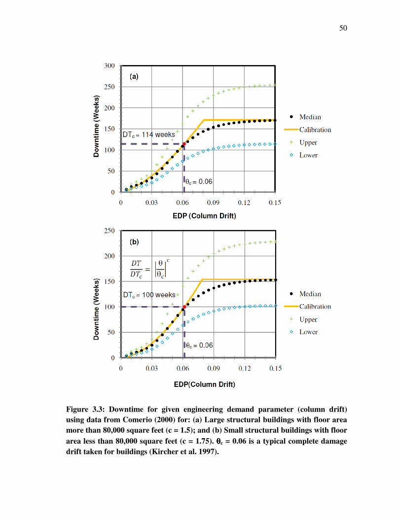
point, θc. All calibrated curves have the same power of c = 2.5.............. 49 Figure 3.3 Downtime for given engineering demand parameter (column drift)

using data from Comerio (2000) for: (a) Large structural buildings with floor area more than 80,000 square feet (c =1.5); and (b) Small structural buildings with floor area less than 80,000 square feet

(c = 1.75). θc = 0.06 is a typical complete damage drift taken for buildings (Kircher et al. 1997)................................................................. 50

Figure 3.4 Five-span prototype bridge used in study. (a) Bridge piers studied by

Mander et al. (2007) and (b) DAD pier designed for California seismicity (DAD2)................................................................................... 53 Figure 3.5 Comparison of median values of downtime loss on log-log scale for

three different design systems Caltrans, DAD2 and Non-Seismic using four-step approach.......................................................................... 54 Figure 3.6 Comparison of median values of downtime loss on log-log scale for

three different design systems New Zealand, DAD1 and Japan using four-step approach.......................................................................... 55 Figure 3.7 Comparative study of expected annual 3D losses of various prototype bridges...................................................................................................... 59 Figure 3.8 Comparative study of 3D losses for scenario event (DBE and MCE) for Non-Seismic and Caltrans prototype bridges..................................... 59 Figure 3.9 Swing analysis with variation of 10% of different parameters for calculation of expected annual downtime losses for DAD1.................... 61 Figure 3.10 Swing analysis with variation of 10% of different parameters for

calculation of total expected annual losses for prototype DAD2 bridge...................................................................................................... . 61

x

LIST OF TABLES

Page Table 2.1 Calculation of expected annual death loss and fatal accident rate (FAR)........................................................................................................ 36 Table 3.1 Definition of damage states and performance outcomes (Mander and Basoz 1999).............................................................................................. 46 Table 3.2 Calculation of expected annual downtime (in Days) for different bridge designs along with median and mean parameters.......................... 56 Table 3.3 Comparative study of a prototype bridge showing total loss (Damage, Death and Downtime) per year for different bridge designs.................... 57 Table 3.4 Comparative study of scenario results for DBE and MCE in California

seismicity.................................................................................................. 58 Table 3.5 3D losses for to prototype bridge in monetary terms for DBE and MCE scenarios.................................................................................................... 58

1

1. INTRODUCTION

1.1 Background and Motivation

Earthquakes are one of the most hazardous natural events which may cause

devastation without warning. Losses due to these types of catastrophes can be

characterized in terms of the 3D’s: Damage, Death and Downtime. Performance-based

earthquake engineering (PBEE) consider these 3D’s as Performance measures. As such

they should also be addressed in loss estimation procedures as the repair cost will not

only be the direct “loss” suffered damage to the owner, but also indirect losses to users

in terms of death and downtime. Thus total losses strictly represent the sum of both

direct and indirect losses that necessitate repair or rebuilding due to earthquake effects.

Generally, only implied losses from structural damage are considered for the design of

infrastructure.

The conventional definition of risk is the product of the probability of the

hazardous event and its associated consequences (Stewart 2009). This definition is

consistent with that used by the US Department of Homeland Security (DHS) National

Infrastructure Protection Plan where risk is assessed from any scenario as a function of

consequence, vulnerability, and threat (DHS 2009). Thus it is important for stakeholders

to know potential downtime and potential fatalities due to collapse of the facility along

with damage repair/replacement costs. This will help a responsible owner to mitigate the

risk to the greatest extent possible.

__________ This thesis follows the style of Journal of Structural Engineering.

2

Recently, Mander and Sircar (2009) and Sircar et al. (2009) developed a four-

step approach to assess the direct financial losses arising from structural damage to

constructed facilities. Although the approach is general and could be applied to any type

of hazard, Sircar et al. (2009) focused on earthquake hazards. Moreover, it is considered

that the four-step approach can be extended to encompass death and downtime. This will

enable the calculation of total “3D-losses” as the model follows similar steps. The

objective of using the Mander and Sircar (2009) direct four-step approach for computing

losses is to relate estimated losses in terms of well-known seismic demand and structural

capacity factors. The loss estimation framework is divided into four interrelated steps:

(a) hazard analysis, (b) structural analysis, (c) damage/loss analysis; and (d) loss

estimation. When these losses are integrated over all possible seismic scenarios, the

Expected Annual Loss (EAL) can be computed directly in terms of a simple formula.

In this research the direct four-step analysis process is extended for the

estimation of death and downtime losses. The approach to incorporate the indirect losses

of death and downtime mirrors what Mander and Sircar (2009) did for physical damage

loss estimation as follows: First, an intensity measure (IM) of hazard such as

acceleration is related to its rate of occurrence (or annual frequency fa or return period

for earthquakes). Second, the earthquake IM is related to the response of the structure

via engineering demand parameters (EDP) such as structural drift (θ); this depends on

the type of structure and its design detailing. These first two steps are common in

estimating each of the 3D’s. The third step is to associate response of the structure with

3

corresponding losses. This can be performed by integrating vulnerability curves over

various damage states to corresponding losses in terms of each of the 3D’s: Damage,

Death and Downtime. The fourth and final step is to associate losses with the hazard

frequency; this can be easily performed by relating the first three steps using a single

compound formula as proposed by Mander and Sircar (2009). The expected annual

losses for the 3D’s can be estimated by integrating losses from their onset over all

possible scenarios.

The objective of this thesis is to develop loss models for Death and Downtime as

an extension of the Mander and Sircar (2009) approach for Damage. Examples will be

drawn from bridges of different design standards and seismic regions.

1.2 Literature Review

1.2.1 Seismic Hazard, Risk and Loss

Low probability-high consequence events like earthquakes have a potential to

cause losses, both structural and non-structural in terms of life, property damage and

facility downtime. It is equally important to predict and mitigate the losses over the

period of time. A predictive capability should help in preparing for the worst to come

and inform owner/users about risk to the facility. As physical damage is a direct loss, it

has always been a primary focus for engineers and others to study the consequences of a

hazardous event. Determining the risk at the site of structural project is the first step in a

performance based design.

Cornell (1968) introduced a method for the evaluation of the seismic risk in

terms of a ground motion parameter (peak ground acceleration) versus average return

4

period at the site of an engineering project. This was a first step in the direction of a

probabilistic risk assessment methodology. Later, Algermissen (1972) studied losses in

the San Francisco Bay area so as to provide the California Office of Emergency Services

on the possible losses produced by large, damaging earthquakes. This was when

California Office of Emergency Services started thinking of some rational basis for state

rescue and recovery operations for future.

Kennedy et al. (1980) studied probabilistic seismic safety of Oyster Creek

nuclear power plant. They considered earthquake hazard as an initiating event that could

result in radioactive release based on probability of earthquake and probability of failure

because of the event. Then, Kennedy and Ravindra (1984) extended their work on

nuclear power plant risk studies using seismic fragilities. They developed seismic

fragilities of critical structures and equipment as families of conditional failure

frequency curves plotted against peak ground acceleration to use in a probability risk

assessment. But sensitivity studies need to be conducted to judge the influence of

different assumptions on risk estimates. Sometime later, Kennedy (1999) worked on risk

based seismic design criteria by aiming certain desired seismic risk in terms of an annual

probability of seismic-induced failure. The integral part of the framework was to

establish the acceptable seismic margin above the design Safe-Shutdown-Earthquake

(SSE) response spectrum. Garrick and Christie (2002) practiced probability risk

assessment technique on nuclear power plants in USA. This signaled the beginning of a

revolution in the licensing process of commercial nuclear power plants.

5

In 1989, the U.S. Federal Emergency Management Agency (FEMA) prepared a

report on estimating losses from future earthquakes and presented it to the National

Academy of Science (NAS). This report may be considered as a cornerstone for carrying

out loss estimation method development and studies. The National Institute of Building

Sciences (NIBS 1994) assessed the state-of-the-art earthquake of loss estimation

methodologies. Thereafter, FEMA collaborated with National Institute of Building

Science (NIBS) and started developing a standard nationally applicable seismic loss

estimation framework on a regional basis (Whitman et al. 1997). The framework is

developed and embodied in geographical information system (GIS) MapInfo-based

software called HAZUS.

HAZUS (1997) was the first edition of risk assessment software package built on

GIS technology, used for mapping and displaying hazard data and the results of damage

and economic loss estimates for building and infrastructure. Kircher et al. (1997) used

building damage functions developed by Whitman et al. (1997) for earthquake loss

estimation. These functions estimate the probability of discrete states of structural and

nonstructural building damage and hence estimate building losses. Thereafter, Mander

and Basoz (1999) developed the seismic fragility curves for highway bridges through the

use of rapid analysis procedures. This was based on fundamentals of mechanics and

dynamics and data obtained from the National Bridge Inventory. The fragility curves

were used to associate losses in terms of its discrete damage states.

HAZUS (2003) was developed as an upgraded version of HAZUS (1997) which

can assess potential losses from multi hazards like floods, hurricanes and earthquakes.

6

Kircher (2003) described procedures based on and compatible with HAZUS that may be

used to develop earthquake damage and related loss functions for welded steel moment-

frame buildings. But an experienced structural engineer is needed to carry out the

process.

Shome and Cornell (1999) developed a relationship between seismic demands on

structures in terms of ground motion parameters which is part of the second step of the

performance based design model. They worked on probabilistic seismic demand analysis

of nonlinear structures in terms of ground motion parameters and frequency of

earthquake. Thereafter, Cornell and Krawinkler (2000) described the foundation on

which performance assessment is based and the major challenges like defining the

objectives of seismic performance assessment (to go for general methodology for

estimating the annualized expected costs or the structure should be compatible for

retrofit which leads to evaluation of design alternatives) on the way to expected success.

Porter et al. (2001) worked on assembly-based vulnerability framework for

evaluating the seismic vulnerability and performance of building. The framework applies

the ground motion time history to structural model to determine structural response and

then utilizes the damage to individual building components to estimate the total loss. The

framework and simulation approach is fully probabilistic and addresses damage in a

highly detailed manner and is building specific. The approach does not rely extensively

on expert opinion but this comes with a cost of rigorous structural analysis and creating

building assemblies and their capacity. Later on, Vamvatsikos and Cornell (2002)

proposed the Incremental Dynamic Analysis (IDA) method, which offers thorough

7

seismic demand and capacity prediction capability by using a series of nonlinear

dynamic analyses under a multiply scaled suite of ground motion records. But selecting

a suite of earthquakes at the desired location/distance from fault is very important as

results may largely depend on it.

Porter et al. (2004) worked on economic seismic risk estimation for buildings

using three different ways; 1) Integration of seismic vulnerability and hazard, 2)

Probable frequency loss and 3) Linear assembly-based vulnerability (LABV). LABV is

similar to four-step rapid modeling process with a striking difference as it simplifies the

analysis of the 50-year loss using linear spectral analysis. They expressed that probable

maximum loss (PML) has no place in a standard financial analysis and need to replace

with more meaningful and applicable term like probable frequent loss (PFL) or expected

annual loss (EAL). They estimated EAL using linear assembly-based vulnerability

(LABV) for number of wood-frame buildings.

Goulet et al. (2007) evaluated seismic performance assessment in terms of

economic losses and collapse safety of a reinforced concrete moment frame building

designed for building code provision (2003). Their work suggests that while considering

higher hazards levels, it is important to consider response spectral shape otherwise it

leads to overestimation of mean annual collapse rate by a factor of 5-10. Later, Baker

and Cornell (2008) worked on determining aleatory and epistemic uncertainty (inherent

randomness and model uncertainty) in each stage of seismic loss estimation framework

and its propagation through the analysis. Mackie et al. (2009) proposed improvement on

previous bridge loss models by local linearization of the dependence between repair

8

quantities and damage states so that the resulting model follows a linear relationship

between damage states and repair points. But this becomes more complicated when the

structure is large and complex.

Dhakal and Mander (2006) expanded upon the idea of the Pacific Earthquake

Engineering Research (PEER) triple integral to include losses in a total probabilistic

framework. Their resulting quadruple integral led to the quantification of the expected

annual financial loss (EAL) for engineered facilities for any natural hazard. At the same

time, Dhakal et al. (2006) worked extensively on seismic financial risk analysis of

reinforced concrete buildings and demonstrated major shortcomings in existing

construction practice. They also showed that improved detailing gives a significant

economic payback in terms of drastically reduced financial risk.

Solberg (2007) performed experimental and computational tests on precast

concrete structures designed for damage avoidance. DAD structures accommodate non-

linear behavior by rocking at specially detailed connections and unbounded prestress is

employed to provide restoring force and supplemental devices are used to dissipate

energy. The EAL of a bridge pier designed for damage avoidance is approximately 25

percent of that of a conventional ductile. Subsequently, Mander et al. (2007) applied

incremental dynamic analysis (IDA) to investigate expected structural response, damage

outcomes, and financial loss from bridges. The results showed that ductility may have

some effect on seismic safety of New Zealand bridges but it is not an alternative to

strength. Later, Solberg et al. (2008) presented a simplified method for EAL without

conducting non-linear dynamic analysis. They proposed a Rapid IDA-EAL method. This

9

was shown to be a powerful, yet simple approach and shows good agreement with the

more comprehensive but time consuming computational IDA-EAL method. They

applied the model to two highway bridge piers; one traditionally designed for ductility

and the other based on DAD.

Bradley et al. (2007) improved seismic hazard model for use in performance-

based earthquake engineering and illustrated the significance of the proposed model on a

typical bridge via probabilistic seismic demand analysis. They have also considered

propagation of epistemic uncertainty in the seismic hazard and compared the model with

power law relationship to illustrate its effects on the risk assessment. The drawback of

the model was that it does not model the response in the region of global collapse.

Mander and Sircar (2009) and Sircar et al. (2009) developed a four-step approach

to assess the direct financial losses arising from physical damage to constructed

facilities. They observed that four-step probabilistic loss model is visually interrelated

through log-log graphs. These losses for each damage states take into account epistemic

uncertainty as well as the effect for loss (cost, downtime and death) surge following a

major hazardous event. The model considered 30% price surge due to inflation in prices

of material and labor in the wake of devastating earthquake. They also considered 10%

swing in various parameters to estimate the change in estimated annual losses per

million dollars of assets. Their inter-relationship via power equations leads to straight

lines between specified coordinates. The four steps can be unified into one single

compound equation which takes the generalized form. Full details of this model are

given in Section 2 and Section 3.

10

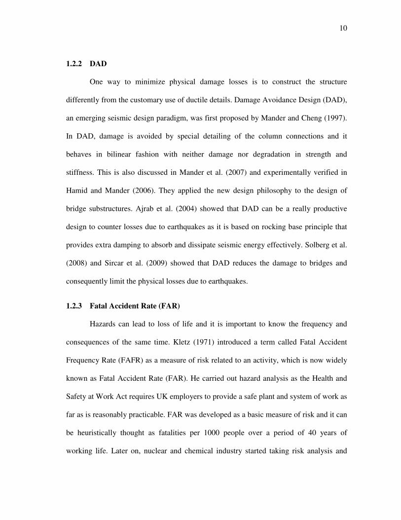
1.2.2 DAD

One way to minimize physical damage losses is to construct the structure

differently from the customary use of ductile details. Damage Avoidance Design (DAD),

an emerging seismic design paradigm, was first proposed by Mander and Cheng (1997).

In DAD, damage is avoided by special detailing of the column connections and it

behaves in bilinear fashion with neither damage nor degradation in strength and

stiffness. This is also discussed in Mander et al. (2007) and experimentally verified in

Hamid and Mander (2006). They applied the new design philosophy to the design of

bridge substructures. Ajrab et al. (2004) showed that DAD can be a really productive

design to counter losses due to earthquakes as it is based on rocking base principle that

provides extra damping to absorb and dissipate seismic energy effectively. Solberg et al.

(2008) and Sircar et al. (2009) showed that DAD reduces the damage to bridges and

consequently limit the physical losses due to earthquakes.

1.2.3 Fatal Accident Rate (FAR)

Hazards can lead to loss of life and it is important to know the frequency and

consequences of the same time. Kletz (1971) introduced a term called Fatal Accident

Frequency Rate (FAFR) as a measure of risk related to an activity, which is now widely

known as Fatal Accident Rate (FAR). He carried out hazard analysis as the Health and

Safety at Work Act requires UK employers to provide a safe plant and system of work as

far as is reasonably practicable. FAR was developed as a basic measure of risk and it can

be heuristically thought as fatalities per 1000 people over a period of 40 years of

working life. Later on, nuclear and chemical industry started taking risk analysis and

11

hazard assessment seriously (Lawley and Kletz (1975); Gibson (1976); Griffiths (1978);

Dunster and Vinck (1979); Lawley (1980); Kennedy et al. (1980); Kennedy and

Ravindra (1984)).

Kletz (1978), Lees (1980) and Elms and Mander (1990) developed some typical

FAR values for various activity or risk exposure. They explained that risk exposure

depends on the activity of a person at the time of disaster. Elms and Mander (1990) used

FAR as a measure of risk to railway locomotive engineers who are exposed to recurring

hazards while driving trains and are affected by various hazards such as slips, floods,

speeding, signal, mechanical and track faults and sleep deprivation.

Subsequently, Mander and Elms (1994) worked on quantitative risk assessment

of large structural systems. They used multiple fault and event trees to evaluate the

probability of fatality from bridge and building collapse due to a catastrophic

earthquake. They applied a similar analogy in various situations like locomotive

collision with an obstruction (Figure 1.1). Even a sleeping person has a latent risk

exposure and this has a measured value of FAR = 1.

1.2.4 Value of Statistical Life (VSL)

Rice and Cooper (1967) estimated value of human life expressed in terms of

lifetime earnings. It was calculated to compare the social benefits associated with

investments in particular programs such as the highway construction, accident control,

education, flood control etc. Later, Acton (1976) and Jones-Lee (1976) measured the

monetary value of life saving programs as economic analysis. Thaler and Sherwin

(1976) and Viscusi (1978) viewed value of saving a life using evidence from the labor

12

market. Rhoads (1978) calculated how much should be spent to save a life through

various models like: 1) Discounted future earnings and 2) Willingness to pay.

Linnerooth (1979) reviewed the models to estimate the value of human life and

suggested some drawbacks and modification for each model. Henley and Kumamoto

(1992) mentioned the outcome of risk study that as risk diminishes to less than 10-6/

year, the average individual does not show undue concern, and so elaborate precautions

against this risk level are seldom taken. For example, this is roughly the probability that

a person can be hit by lightning.

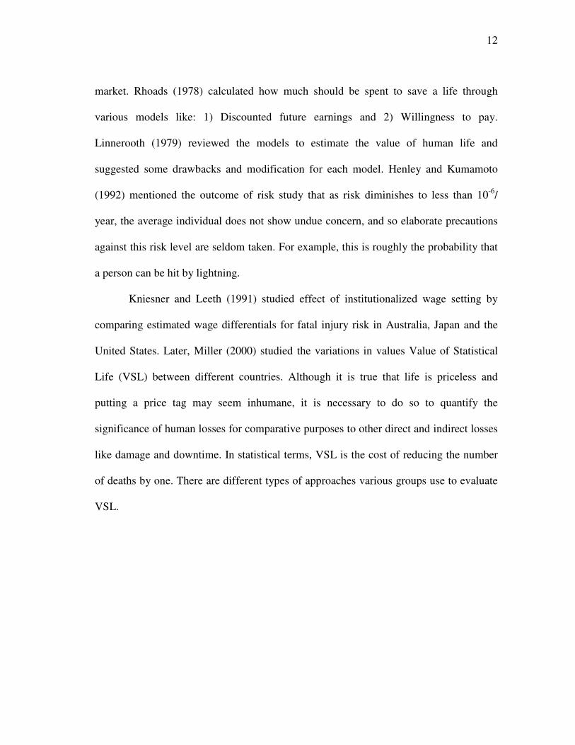
Kniesner and Leeth (1991) studied effect of institutionalized wage setting by

comparing estimated wage differentials for fatal injury risk in Australia, Japan and the

United States. Later, Miller (2000) studied the variations in values Value of Statistical

Life (VSL) between different countries. Although it is true that life is priceless and

putting a price tag may seem inhumane, it is necessary to do so to quantify the

significance of human losses for comparative purposes to other direct and indirect losses

like damage and downtime. In statistical terms, VSL is the cost of reducing the number

of deaths by one. There are different types of approaches various groups use to evaluate

VSL.

13

Figure 1.1: Fault and event trees for a locomotive collision with an obstruction

(Mander and Elms 1994).

14

The U.S. Department of Transportation (2007) has suggested VSL = $5.8

million. Such a VSL is a mean value of various studies carried out by five different

people over the period of four years. Another governmental agency, Environmental

Protection Agency (EPA) has suggested that VSL = $6.9 million in 2008. Kniesner et al.

(2009) examined the differences in the VSL across potential wage levels in panel data

using quantile regressions with intercept heterogeneity. Their findings indicate that a

reasonable average cost per expected life saved cut-off for health and safety regulations

in $7 million to $ 8 million. Based on the above, as of the time of writing a value of VSL

= $ 6.0 million shall be used in this work.

1.2.5 Downtime

Basoz and Mander (1999) developed fragility curves for the highway

transportation lifeline module of HAZUS. They developed a complete description on the

theoretical background of the damage functions and associated each damage state with

corresponding downtime. From this downtime losses could be assessed. Beck et al.

(1999) developed a methodology modified from a repair-time model to estimate the

rational component of downtime. The remaining portion of structure downtime is

difficult to model because it is highly dependent on irrational components.

Comerio (2000) expressed that downtime includes the time necessary to plan,

finance and complete repair of facilities damaged in earthquakes or other disasters. She

goes on to point out there are various factors that can affect downtime: structural

inspection, damage assessment, finance planning, architect/engineering consultations, a

15

possible competitive bidding process, and the repair effort need to return a structure back

to its undamaged state (Comerio 2006).

The rational components of facility downtime are attributed to the time needed to

repair building damage. This is also an essential part of loss modeling, because it is one

measure of operational failure in a lifeline or the business interruption loss in buildings.

Comerio considered the University of California Berkeley as an experimental region and

the losses after the 1994 Northridge earthquake were used to calibrate her models. A

simplified method for estimating downtime was developed based on the floor area of

buildings.

1.3 Scope of Thesis

The scope of the thesis is outlined below:

i. To develop the empirically calibrated four-step model for estimating annual

losses in terms of expected death and downtime based on the four-step

approach of Mander and Sircar (2009).

ii. To calculate FAR and estimate annual death losses in monetary terms using

VSL. Also, to associate downtime with financial losses for different kinds of

bridge structures.

iii. To prepare DAD bridge design according to California design code and

seismicity and its response for a given intensity measure in terms of drift.

iv. For a prototype bridge, compare and aggregate the 3D losses from different

designs and detailing (non-seismic, seismic and DAD) using examples based

on California and New Zealand seismicity along with Japan design standards.

16

1.4 What Then Is Particularly New in This Thesis?

The particularly new work presented in what follows is outlined below:

i. Historically, engineers have fixated on quantifying the extent of physical damage

losses through fragility analysis; death and downtime have only been paid scant

attention. This thesis seeks to redress this imbalanced view.

ii. As it is important to develop a common and easy method to estimate death and

downtime losses along with damage, the four-step approach proposed by Mander

and Sircar (2009) has been extended accordingly.

iii. To compare 3D (death, downtime, damage) losses on one scale in order to study

the relative importance of each. VSL and downtime cost in terms of annualized

dollar losses is used to convert death and downtime into monetary terms,

respectively.

iv. The extended 3D seismic loss analysis is applied to the bridges studied by

Solberg et al. (2008). Thus examples of historic non-seismically designed

structures along with conventionally designed ductile seismic resistant structures

and the emerging damage avoidance design (DAD) class of structures are

investigated.

17

2. RAPID LOSS MODELING OF FATALITIES CAUSED BY SEISMICALLY

DAMAGED STRUCTURES

2.1 Summary

Structural design codes and specifications are primarily concerned with

preserving life-safety. But these are not accordingly calibrated in a direct probabilistic

risk or life-safety context. In this section a probabilistic fatality rate framework is

developed for structures where seismic hazard is related to structural response, which is

then related to damage and collapse, which in turn is related to the potential for fatality.

The model is a power curve and calibrated using event and fault trees. The power curve

is copped with lower and upper bounds, the former relates to damage onset while the

latter corresponds to complete damage (damage state 5, toppling or collapse). The utility

of the approach is investigated for bridges and the calibrated model is validated with

Caltrans, Japan, New Zealand bridges along with Damage Avoidance Design (DAD),

Seismic and Non-seismic designed structures. Result shows that Fatal Accident Rate

(FAR) for DAD is very low while for non-seismically design structures it is seven times

higher. The results are then converted into monetary terms using the value of statistical

life (VSL).

2.2 Introduction

Failure of an engineered structural system may lead to direct and collateral

damages, that is: physical damage to the constructed facility; loss of life or limb; and

down-time within the system leading to loss of revenue and profit. Often engineers

18

disregard the consequences of failure while focusing on the preservation of life-safety

via collapse prevention for a maximum considered design event such as an earthquake

with a return period of say 1000 years. It is important to not only communicate the risk

to life and limb associated with structural damage but stakeholders also need to know the

indirect financial losses along with the long-term economic losses arising from

downtime. The objective of this section is to develop a simplified procedure that directly

relates hazard intensity to response of the structure through collapse and hence to the

chance of fatality.

A quantitative risk assessment technique is proposed to examine the risk to life

and computed in terms of the well-known Fatal Accident Rate (FAR). A four-step

approach is used which can be subdivided into four distinct tasks; (a) hazard analysis;

(b) structural analysis; (c) damage and hence fatality analysis; and (d) FAR estimation.

Recent research has shown that combination of fragility curves with loss functions can

be used for probabilistic risk assessment methodology to estimate expected annual

financial loss for structure (Kircher et al. 1997; Dhakal et al. 2006; Mander et al. 2007;

Solberg et al. 2008). More recently a direct rapid loss assessment approach has been

proposed by Mander and Sircar (2009) and Sircar et al. (2009) for earthquake induced

damage to buildings and bridges.

The first step involves determination of seismic hazard at the constructed facility

site by developing a relationship between earthquake intensity measures (IM) and its

annual frequency, the inverse of which is return period. Such a model needs to be based

on all seismic hazards (and thus faults) at a site, and therefore the general seismicity of a

19

region with predictions based on existing historic catalogue information and models.

Similarly, the second step relates IM with structural response in terms of engineering

demand parameters (EDP) such as drift (θ). The third step involves associating EDP

with probability of fatality using fragility curves. This is accomplished by associating

damage states with an EDP in terms of drift and later on, associating losses at those

drifts. The fourth and final step is inter-relating the first three-steps and integrating

losses over the entire range of frequency. Then these losses can be converted into the

well-known parameter, FAR. Each of these relationships involves uncertainty and must

be treated probabilistically from location, seismic demand versus capacity, and capacity

versus fatality.

FAR is the common measure to describe potential for fatalities and it can be

thought as number of fatalities per 1000 lives over a period of 40 years due to an event

or activity with 2500 hours every year. It is transient in nature as exposure changes from

structure to structure and activity to activity. General risk for a specific activity is given

by a composite FAR. This can be disaggregated into components of the risk which may

arise from different failure modes or accident types. There is need to develop a method

that relates probability of fatality to an EDP through a simple relationship in order to

rapidly determine the probability of a fatality for a specific scenario earthquake event as

well as overall FAR.

The aim of this work is to develop a closed form fatality estimation framework

that directly relates (a) hazard to (b) structural response to (c) damage and losses (d) and

hence to fatality probability. Note that customary evaluation of convolution integrals is

20

not needed in this direct approach. The proposed closed form framework for the fatality

estimation procedure is derived extensively from recent work by Mander and Sircar

(2009) along with quantitative risk assessment work by Mander and Elms (1994) that

produced fatality estimates.

The present section applies the framework to the failure of transportation

structures, specifically bridges designed to different specifications and more specifically,

contrasting non-seismic, seismic and emerging DAD philosophies.

2.3 Direct Loss Estimation Framework

This framework is used by Mander and Sircar (2009) for financial loss analysis

of seismically damaged buildings. It is a quantitative four-step process to estimate the

expected annual losses for different types of structure. Figure 2.1 shows the four-step

framework along with its connectivity between each step. The inter-relationships may be

approximated as capped linear functions in log-log space. The main objective of using

the direct four-step procedure is to relate the probability of loss of life with well-known

seismic demand and structural capacity parameters.

21

Figure 2.1: Summary of the Four-step approach used to estimate loss. (a) Two

points on hazard recurrence curve are used to compute the IM (hazard analysis).

(b) The IM’s derived from (a) Are used to compute inter-story drifts using the

hazard-drift curve (structural analysis). (c) The drifts obtained from (b) Are used

to compute death loss (d) From which loss is computed.

22

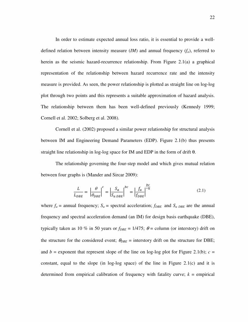
In order to estimate expected annual loss ratio, it is essential to provide a well-

defined relation between intensity measure (IM) and annual frequency (fa), referred to

herein as the seismic hazard-recurrence relationship. From Figure 2.1(a) a graphical

representation of the relationship between hazard recurrence rate and the intensity

measure is provided. As seen, the power relationship is plotted as straight line on log-log

plot through two points and this represents a suitable approximation of hazard analysis.

The relationship between them has been well-defined previously (Kennedy 1999;

Cornell et al. 2002; Solberg et al. 2008).

Cornell et al. (2002) proposed a similar power relationship for structural analysis

between IM and Engineering Demand Parameters (EDP). Figure 2.1(b) thus presents

straight line relationship in log-log space for IM and EDP in the form of drift θ.

The relationship governing the four-step model and which gives mutual relation

between four graphs is (Mander and Sircar 2009):

����� = � θ

���� = � ������ = � �������� �

(2.1)

where fa = annual frequency; Sa = spectral acceleration; fDBE and Sa DBE are the annual

frequency and spectral acceleration demand (an IM) for design basis earthquake (DBE),

typically taken as 10 % in 50 years or fDBE = 1/475; θ = column (or interstory) drift on

the structure for the considered event; θDBE = interstory drift on the structure for DBE;

and b = exponent that represent slope of the line on log-log plot for Figure 2.1(b); c =

constant, equal to the slope (in log-log space) of the line in Figure 2.1(c) and it is

determined from empirical calibration of frequency with fatality curve; k = empirical

23

seismic hazard constant; L = physical damage loss ratio; LDBE = losses corresponding to

design basis earthquake. The exponent of Figure 2.1(d), d, is inter-related to the first

three powers as:

� = ��−� (2.2)

They proposed two-parameter power curve with upper and lower cutoffs to

represent a loss ratio as a function EDP. The empirical model is expressed as:

��� = � θ

θ��� ; ��� ≤ � ≤ �� = 1.3 (2.3)

in which θ = column lateral drift (the EDP); θc = f θDB5 critical drift (where f =

adjustment factor for low damage structures where f > 1, generally f = 1, but this may

have a different value for certain special structure types; and θDB5 = drift value for onset

of complete damage); L = loss ratio for a given drift (θ); Lc = unit cost (normally Lc = 1,

at onset of complete damage; Damage State 5); Lon = loss ratio at onset of damage state

2; Lu = loss ratio at complete damage or toppling of structure (30% more to allow price

surge).

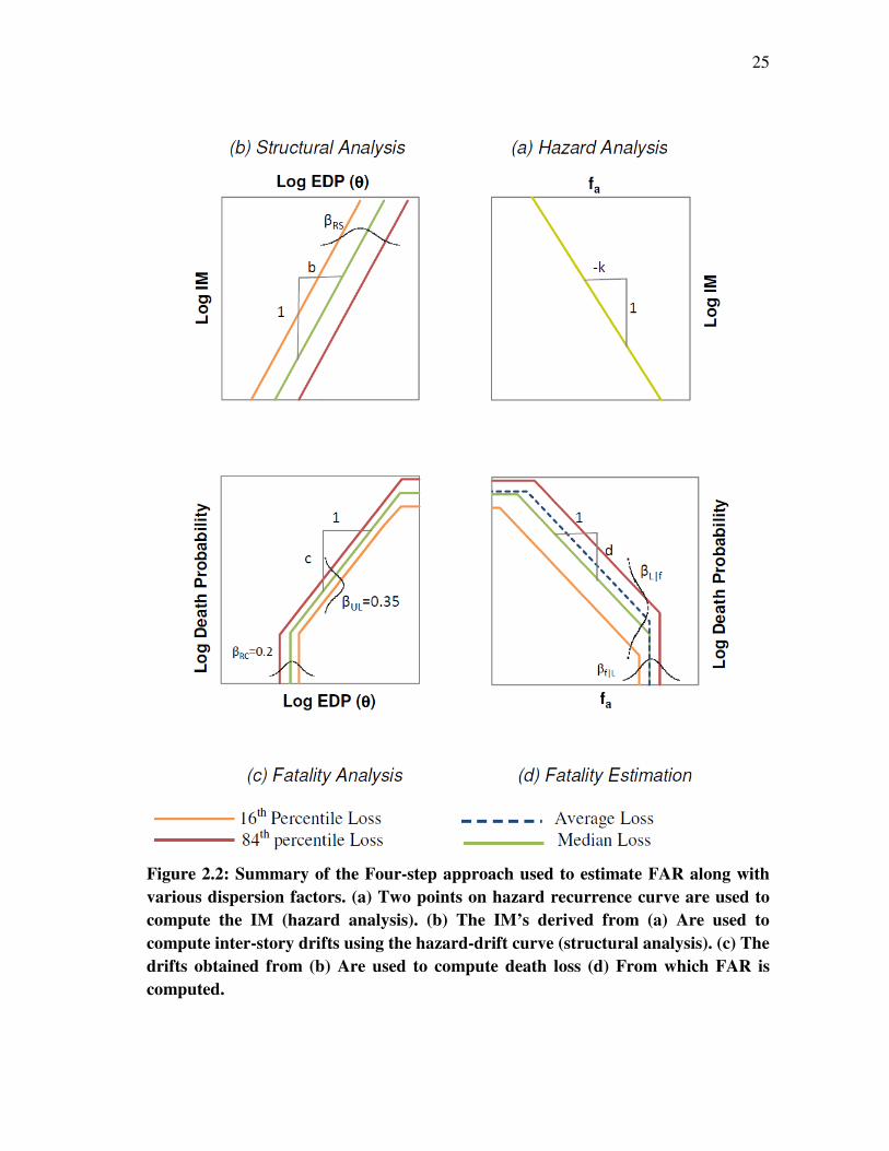
2.4 Proposed Death Loss Model

Previously Shiono et al. (1995) showed that fatality follows a log-log linear

(power) relationship with collapse rate of building. Thus fatality model developed uses

similar type of power relationship as it is been developed for physical damage losses

(Mander and Sircar 2009) and shown in Figure 2.2 along with various dispersion factors.

Briefly, the four-step death loss model directly estimates losses due to inter-relationships

between (a) hazard, (b) structural response, (c) damage and (d) death loss:

24

������� = � θ

���� = � ������ = � �������� �

(2.4)

in which DL = probability of death loss; DLDBE = probability of death loss at design basis

earthquake.

As the probability of death loss associated with each damage state is not

distinctly defined, so the model is calibrated using probable death loss at the onset of

Damage State 5 (complete collapse or toppling). The model is then bounded with upper

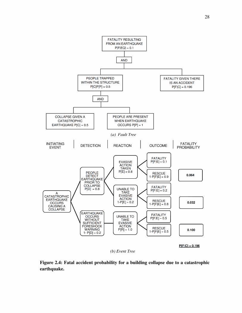
and lower cutoffs based on structural drift. Figures 2.3 and 2.4 uses fault and event trees

to analyse the probability of death loss due to a catastrophic earthquake for bridges and

buildings, respectively. Chance of fatality at onset of complete damage (drift

corresponding to onset of Damage State 5) is taken as 10% for building and bridges

(Mander and Elms 1994). The empirical death loss model with upper and lower cutoff

takes the form as shown:

����� = � θ

θ��� ���; ���� ≤ �� ≤ ��� = 0.75 (2.5)

in which DLc = probability of death loss for drift corresponds to the onset of complete

damage; DLon = probability of death loss at onset of Damage State 2; DLu = ultimate

probability of death loss (at complete damage or toppling of structure).

25

Figure 2.2: Summary of the Four-step approach used to estimate FAR along with

various dispersion factors. (a) Two points on hazard recurrence curve are used to

compute the IM (hazard analysis). (b) The IM’s derived from (a) Are used to

compute inter-story drifts using the hazard-drift curve (structural analysis). (c) The

drifts obtained from (b) Are used to compute death loss (d) From which FAR is

computed.

26

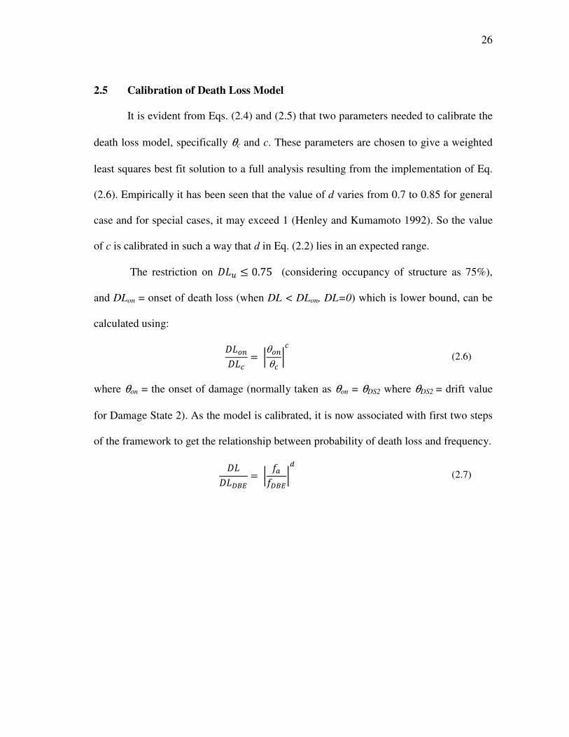
2.5 Calibration of Death Loss Model

It is evident from Eqs. (2.4) and (2.5) that two parameters needed to calibrate the

death loss model, specifically θc and c. These parameters are chosen to give a weighted

least squares best fit solution to a full analysis resulting from the implementation of Eq.

(2.6). Empirically it has been seen that the value of d varies from 0.7 to 0.85 for general

case and for special cases, it may exceed 1 (Henley and Kumamoto 1992). So the value

of c is calibrated in such a way that d in Eq. (2.2) lies in an expected range.

The restriction on ��� ≤ 0.75 (considering occupancy of structure as 75%),

and DLon = onset of death loss (when DL < DLon, DL=0) which is lower bound, can be

calculated using:

������� = �θ��θ� ��

(2.6)

where θon = the onset of damage (normally taken as θon = θDS2 where θDS2 = drift value

for Damage State 2). As the model is calibrated, it is now associated with first two steps

of the framework to get the relationship between probability of death loss and frequency.

������� = � ������"

(2.7)

27

Figure 2.3: Fatal accident probability for a bridge collapse due to a catastrophic

earthquake.

28

Figure 2.4: Fatal accident probability for a building collapse due to a catastrophic

earthquake.

29

All the equations are probabilistic and values of parameters have an uncertainty

and randomness associate with them so it is necessary to incorporate the effects of

variability. It involves in both estimating the demand over time produced by the

earthquake ground motion and the capacity of structure to resist those demands (Cornell

et. al 2002). In this, randomness and uncertainty are considered as aleatoric and

epistemic, respectively. Similarly the probability of death loss in Eq. (2.4) contains both

aleatoric and epistemic uncertainties. It is essential to transform the median parameters

to other fractiles, including the mean values in order to estimate chances of death loss in

each steps of the model. By quantifying the kind and degree of uncertainty in each of the

parameters concerned, the mean value can be estimated. As the power nature of the

death estimation model, a lognormal distribution shall be assumed as appropriate

representation of variability. Using the approach outlined by (Kennedy et. al 1980), the

total dispersion can be estimated in each of the parameters involved in computing chance

of death loss.

Expected Annual Death Loss (EADL) can be calculated by integrating the area

under the mean curve of Figure 2.2(d) when that curve is plotted to a natural scale. Thus

in integral form EADL may be found by computing following:

#$�� = % �� ��&'(

)= ����� + ����� % + �

����," ��&'(

&- (2.8)

This can be expressed as:

#$�� = . �/����0000�� + ���1 ��0000�1 + � 2 �34 � ≠ −1 (2.9)

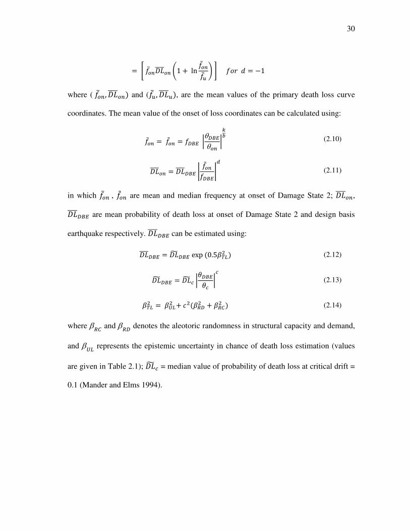
30

= 6 �/����0000�� .1 + ln �/���/� 2 9 �34 � = −1

where ( �/��, ��0000��) and (�/�, ��0000�), are the mean values of the primary death loss curve

coordinates. The mean value of the onset of loss coordinates can be calculated using:

�/�� = �<�� = ���� ���� �

�� (2.10)

��0000�� = ��0000��� = �/������="

(2.11)

in which �/�� , �<�� are mean and median frequency at onset of Damage State 2; ��0000��,

��0000��� are mean probability of death loss at onset of Damage State 2 and design basis

earthquake respectively. ��0000��� can be estimated using:

��0000��� = ��> ��� exp (0.5CDEF ) (2.12)

��> ��� = ��> � �G���G� �� (2.13)

CDEF = CHEF + �F(CI�F + CIJF ) (2.14)

where βIJ and βI� denotes the aleotoric randomness in structural capacity and demand,

and βHE represents the epistemic uncertainty in chance of death loss estimation (values

are given in Table 2.1); ��> � = median value of probability of death loss at critical drift =

0.1 (Mander and Elms 1994).

31

Similarly, the coordinates of death losses corresponding to the mean value of

complete damage can be computed from:

��0000� = ��> � exp (0.5CHEF ) (2.15)

�/� = ���� = ��0000���0000���=K" (2.16)

FAR can be calculated from using EADL from Eq. (2.9) by:

L$M = 11400 (#$��) (2.17)

where numerical coefficient of 11400 converts the EADL into the well known definition

of FAR.

2.6 Bridge-Specific Likelihood of Death Loss

Given a catastrophic event, number of people dying can be estimated using the

probability of death loss multiplying with the average number of people present (Np) in

the danger zone of length (L+S):

OP = � ($$�Q) (� + )24 (1000 S) (2.18)

where n = occupancy of vehicle; AADT = annual average daily traffic; L = Length of

bridge (m); S = approach stopping distance (m); and V = speed of vehicle (km/h).

32

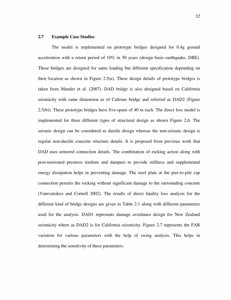
2.7 Example Case Studies

The model is implemented on prototype bridges designed for 0.4g ground

acceleration with a return period of 10% in 50 years (design basis earthquake, DBE).

These bridges are designed for same loading but different specification depending on

their location as shown in Figure 2.5(a). These design details of prototype bridges is

taken from Mander et al. (2007). DAD bridge is also designed based on California

seismicity with same dimension as of Caltrans bridge and referred as DAD2 (Figure

2.5(b)). These prototype bridges have five-spans of 40 m each. The direct loss model is

implemented for three different types of structural design as shown Figure 2.6. The

seismic design can be considered as ductile design whereas the non-seismic design is

regular non-ductile concrete structure details. It is proposed from previous work that

DAD uses armored connection details. The combination of rocking action along with

post-tensioned prestress tendons and dampers to provide stiffness and supplemental

energy dissipation helps in preventing damage. The steel plate at the pier-to-pile cap

connection permits the rocking without significant damage to the surrounding concrete

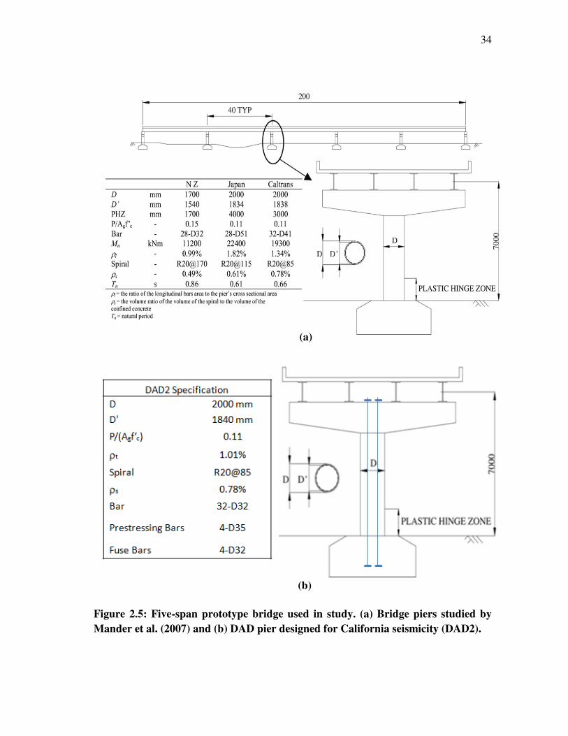
(Vamvatsikos and Cornell 2002). The results of direct fatality loss analysis for the

different kind of bridge designs are given in Table 2.1 along with different parameters

used for the analysis. DAD1 represents damage avoidance design for New Zealand

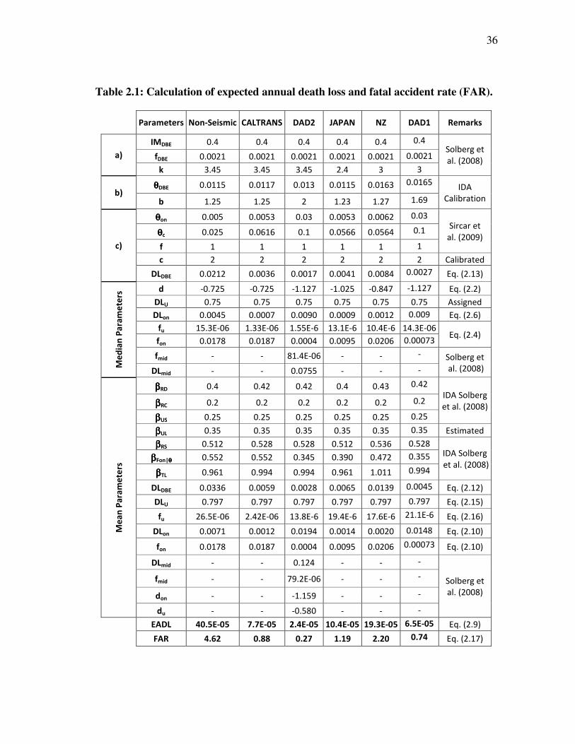
seismicity where as DAD2 is for California seismicity. Figure 2.7 represents the FAR

variation for various parameters with the help of swing analysis. This helps in

determining the sensitivity of these parameters.

33

2.8 Discussion

A probabilistic death estimation framework directly relate hazard to response and

hence to death. This process works really well by taking into account the probability of

death loss due to damage of different earthquake starting from frequent to very rare ones.

The aim of the analysis is to consider the humanitarian background while constructing

the civil engineering structure. Owners don’t want to expose people to more risk just

because they are using their facility. The conceptual design of DAD type structures work

really well during natural hazards like earthquake but these kinds of structures are still

not in use. The model takes into account the different structural strengths and ductility

capabilities and the different seismic-hazard frequency relations. These different

attributes are all integrated in the evaluation of expected annual death loss. This value

helps in calculating FAR, which is good parameter to represent the chance of fatality

over a period of 40 years in laymen terms. From this process, indirect losses in monetary

terms can be measured, which is a missing from previous studies.

34

Figure 2.5: Five-span prototype bridge used in study. (a) Bridge piers studied by

Mander et al. (2007) and (b) DAD pier designed for California seismicity (DAD2).

(a)

(b)

35

Figure 2.6: Analysis of fatalities for different bridge designs and regions on log-log

scale (DAD1 for NZ and DAD2 is for California seismicity respectively).

36

Parameters Non-Seismic CALTRANS DAD2 JAPAN NZ DAD1 Remarks

a)

IMDBE 0.4 0.4 0.4 0.4 0.4 0.4 Solberg et

al. (2008) fDBE 0.0021 0.0021 0.0021 0.0021 0.0021 0.0021

k 3.45 3.45 3.45 2.4 3 3

b) θθθθDBE 0.0115 0.0117 0.013 0.0115 0.0163 0.0165

IDA

Calibration b 1.25 1.25 2 1.23 1.27 1.69

c)

θθθθon 0.005 0.0053 0.03 0.0053 0.0062 0.03 Sircar et

al. (2009) θθθθc 0.025 0.0616 0.1 0.0566 0.0564 0.1

f 1 1 1 1 1 1

c 2 2 2 2 2 2 Calibrated

DLDBE 0.0212 0.0036 0.0017 0.0041 0.0084 0.0027 Eq. (2.13)

Me

dia

n P

ara

me

ters

d -0.725 -0.725 -1.127 -1.025 -0.847 -1.127 Eq. (2.2)

DLU 0.75 0.75 0.75 0.75 0.75 0.75 Assigned

DLon 0.0045 0.0007 0.0090 0.0009 0.0012 0.009 Eq. (2.6)

fu 15.3E-06 1.33E-06 1.55E-6 13.1E-6 10.4E-6 14.3E-06 Eq. (2.4)

fon 0.0178 0.0187 0.0004 0.0095 0.0206 0.00073

fmid - - 81.4E-06 - - - Solberg et

al. (2008) DLmid - - 0.0755 - - -

Me

an

Pa

ram

ete

rs

ββββRD 0.4 0.42 0.42 0.4 0.43 0.42

IDA Solberg

et al. (2008) ββββRC 0.2 0.2 0.2 0.2 0.2 0.2

ββββUS 0.25 0.25 0.25 0.25 0.25 0.25

ββββUL 0.35 0.35 0.35 0.35 0.35 0.35 Estimated

ββββRS 0.512 0.528 0.528 0.512 0.536 0.528 IDA Solberg

et al. (2008) ββββFon|θθθθ 0.552 0.552 0.345 0.390 0.472 0.355

ββββTL 0.961 0.994 0.994 0.961 1.011 0.994

DLDBE 0.0336 0.0059 0.0028 0.0065 0.0139 0.0045 Eq. (2.12)

DLU 0.797 0.797 0.797 0.797 0.797 0.797 Eq. (2.15)

fu 26.5E-06 2.42E-06 13.8E-6 19.4E-6 17.6E-6 21.1E-6 Eq. (2.16)

DLon 0.0071 0.0012 0.0194 0.0014 0.0020 0.0148 Eq. (2.10)

fon 0.0178 0.0187 0.0004 0.0095 0.0206 0.00073 Eq. (2.10)

DLmid - - 0.124 - - -

Solberg et

al. (2008)

fmid - - 79.2E-06 - - -

don - - -1.159 - - -

du - - -0.580 - - -

EADL 40.5E-05 7.7E-05 2.4E-05 10.4E-05 19.3E-05 6.5E-05 Eq. (2.9)

FAR 4.62 0.88 0.27 1.19 2.20 0.74 Eq. (2.17)

Table 2.1: Calculation of expected annual death loss and fatal accident rate (FAR).

37

Figure 2.7: Swing analysis with variation of 10% of different parameters for

calculation of FAR for DAD1.

-30 -20 -10 0 10 20 30

c

θθ θθo

n

θθ θθcr

θθ θθ

DB

Eb

k

38

2.9 Section Closure

From the research presented in this section the following conclusions are drawn:

1. The results for different kind of structures (Seismic, Non-Seismic and DAD)

shows that building structures using DAD technology puts the person on much

lesser risk than person sleeping which is socially needed as no-one wants to

expose more risk just because he is driving on bridge.

2. For Caltrans and Japan Bridge works as seismically designed ones whereas New

Zealand Bridge is can be considered as intermediate designed bridge between

seismic and non-seismic.

3. Probability of a collapse will be sensitive to the structures intrinsic ductility

capability. Also the risk exposure to individual in a building will depend on

where they are located at the time the earthquake strikes and their state of

readiness to take evasive action.

4. In this maximum probability of death is considered to be 75% looks more

realistic, as building is considered to be occupied fully for 2/3 of the time of the

day and remaining time it can be consider as 25% occupied.

39

3. RAPID LOSS MODELING OF DOWNTIME CAUSED BY SEISMICALLY

DAMAGED STRUCTURES

3.1 Summary

Potential design codes and specifications do not include the importance of

structures based on downtime losses arising from catastrophic events such as

earthquakes. This section seeks to display the importance of downtime in an overall

quantitative risk assessment framework. Downtime is referred as the period when a

structure is unavailable or it fails to perform to its capacity. The loss model is developed

by multiplying the probabilities of being in each of the damage states using vulnerability

curves by the corresponding downtime losses and summing those losses across all

damage states to give composite downtime with respect to an engineering demand

parameter, like drift. The losses are then calibrated to a capped power curve. The

calibrated loss model is then incorporated into a direct four-step probabilistic loss

modeling framework. This relates seismic hazard to structural response and hence

structural response to downtime losses from which scenario losses or the expected

annual downtime losses (EADT) for all earthquake hazards are calculated. The

downtime losses are the then converted into equivalent monetary losses for bridge-

specific examples. The utility of the model is demonstrated for bridges from Caltrans

and New Zealand seismicity with different structural detailing. A hypothetical bridge is

used to compare 3D losses for bridge design and scenario event.

40

3.2 Introduction

Natural hazards like earthquakes lead to direct physical damage as well as

indirect losses such as death and downtime. Downtime includes the time necessary to

plan, finance, and complete repairs of facilities damaged in disaster. Downtime losses

can have consequences like delay in reaching the aid to affected people, shut down of

necessary business units like food and medical shops etc. Moreover, downtime if

lengthy, affects a region’s long-term economy. It is important, especially for business

organizations, to determine possible downtime as this may lead to much greater losses

than just physical damage and death.

The objective of this section is to develop a simplified procedure that relates

hazard, to structural response, to downtime and hence estimate losses for key scenario

earthquake events, as well as downtime for all hazards leading to expected annual

downtime losses (EADL). Generally insurance companies cover losses due to physical

damage and death but losses due to downtime may not be covered because compensation

is difficult to assess. This can contribute to financial liabilities to individuals/firm and

hence to shareholders.

Basoz and Mander (1999) developed fragility curves for assessing the seismic

vulnerability of highway bridges through the use of rapid analysis procedures. These

curves can be used in various ways as part of a seismic vulnerability analysis

methodology for highway bridges. Later, Comerio (2000) estimated the downtime for

building structures based on damage states, floor area of building and type of building

(wooden, concrete/brick etc.) of U. C. Berkeley campus. The proposed model estimates

41

downtime losses in similar fashion as Mander and Sircar (2009) did for physical

damage. They used probability risk assessment methodology to estimate EAL using

fragility curve and loss function. After estimating EADL in similar as they did for EAL,

the EADL can be associated to monetary losses depending on the context. For example,

a building owner will lose rent over the downtime period and while residents will have

to pay for shifting and higher rental (price surge) at a new place.

Public assets, such as the highway system are difficult to deal with because

ownership and use is collective, thus downtime effects are distributed throughout society

at large, but the impact is felt most by the users of those facilities. Private bridge owners

will lose toll tax money, whereas public users will have to pay for extra miles and time

need to reroute also there will with wear and tear to that route. This will help in

comparing 3D losses in monetary terms and their relative significance.

After a catastrophic event, it is essential to get back to normal life as soon as

possible. It is desirable for corporations and people want to know the time needed to do

so. Delay time can cause bigger losses than direct damage as people may not be able to

get necessary aid, either in short or long term; this affects the economy of the region.

Often engineers disregard the indirect consequences of structural failure while focusing

on the economical minimization of the probability of structural damage and losses. It is

important to communicate downtime along with physical damage of structure and the

risk of life.

42

Historically, the importance of a structure is an arbitrary assignment of extra

strength by design codes which has been based on engineering judgment and collective

experience rather than rigorous analysis.

Mander and Sircar (2009) worked on quantitative risk assessment technique to

estimate physical damage losses. For that, a four-step probabilistic approach is used

which can be subdivided into four distinct tasks: (a) hazard analysis; (b) structural

analysis; (c) damage and hence loss analysis; and (d) loss estimation. Recent research

has shown that combination of fragility curves with loss functions can be used for

probabilistic risk assessment methodology to estimate expected annual losses for a

structure (Kircher et al. 1997; Dhakal and Mander 2006; Mander et al. 2007; Solberg et

al. 2008; Sircar et al. 2009). The same procedure is extended herein to calculate the

downtime for a given type of structure and earthquake intensity or frequency.

At a constructed facility site, evaluation of seismic hazard and intensity measure

(IM) is required for hazard analysis. Structural analysis involves prediction of structural

response to increasing levels of ground shaking in terms of engineering demand

parameter (EDP). Damage and hence downtime analysis uses EDPs to determine

damage measures to the facility components from which downtime can be estimated.

Each of these relationships involves uncertainty and must be treated probabilistically

from location, seismic demand versus capacity, and capacity versus fatality. The

proposed model is calibrated for buildings (Comerio 2000) from U.C. Berkeley campus

and bridges of different detailing.

43

3.3 Proposed Downtime Loss Model

Figure 3.1 presents the four-step loss modeling approach of Mander and Sircar

(2009) adapted herein for estimating downtime losses for seismically damaged

structures. The main objective of using a direct four-step process for computing losses

is to relate estimated losses in terms of well-known seismic demand and structural

capacity parameters. These four steps are interrelated through use of log-log graphs

from (a) hazard, to (b) response, to (c) damage and (d) hence losses. The relationship

between these graphs can be represented using following equation:

�Q�Q��� = � θ

���� = � ������ = � �������� �

(3.1)

where DT = downtime (weeks) and DTDBE = downtime at design basis earthquake

(weeks). fa = annual frequency; Sa = spectral acceleration; fDBE and Sa DBE are the annual

frequency and spectral acceleration demand (an IM) for design basis earthquake (DBE),

typically taken as 10% in 50 years or fDBE = 1/475. θ is the column (or interstory) drift

on the structure for the considered event; θDBE = interstory drift on the structure for

design basis earthquake; k = best fit empirical constant for figure 3.1(a); b = exponent

that represent slope of the line on log-log plot for figure 3.1(b); c = empirically

calibrated power for figure 3.1(c). The slope of the log-log graph in Figure 3.1 (d) is

related to first three graphs as:

� = ��−� (3.2)

44

Figure 3.1: Summary of the interrelated four-step approach used to estimate

downtime showing, (a) Hazard analysis (b) Structural analysis (c) Downtime

analysis and (d) Downtime estimation.

45

The proposed downtime loss model is a power curve. This also has upper and

lower cut-offs; it can be represented using downtime losses in terms of structural drift.

This relationship can be expressed as:

�Q�Q� = � θ

θ��� ; �Q�� ≤ �Q ≤ �Q� (3.3)

in which �Q� = downtime at onset of damage state 5 (complete damage or toppling); θc

= f θDS5 = the critical drift, where θDS5 = drift value for complete damage (collapse), and f

= factor to adjust for low damage structures. Generally f = 1, but this can have different

values for certain special structure types; �Q� = downtime at complete damage or

toppling, downtime at this point will be maximum and does not increase after that (DT <

DTu = 150 weeks ~ 3 years, for bridges, Mander and Basoz (1999)); �Q�� = lower bound

on downtime is based on the concept that there will be no damage to structure when

earthquake intensity is less than damage state 2 (when DT < DTon, DT =0) and can be

estimated as:

�Q���Q� = �θ��θ� ��

(3.4)

where θon = the onset of damage (normally taken as θon = θDS2 = drift value for Damage

State 2), at this state the structure is expected at least some kind of inspection by experts

which can lead to downtime.

46

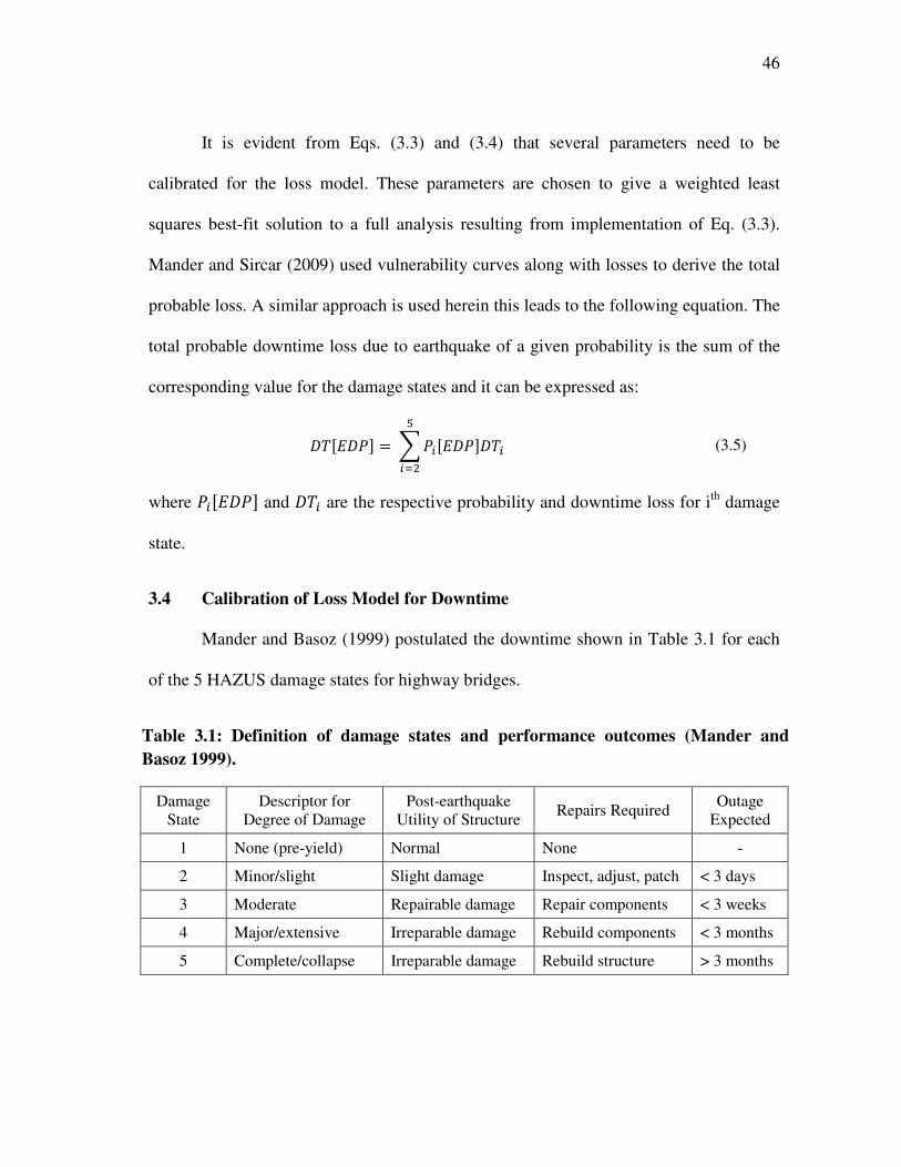
It is evident from Eqs. (3.3) and (3.4) that several parameters need to be

calibrated for the loss model. These parameters are chosen to give a weighted least

squares best-fit solution to a full analysis resulting from implementation of Eq. (3.3).

Mander and Sircar (2009) used vulnerability curves along with losses to derive the total

probable loss. A similar approach is used herein this leads to the following equation. The

total probable downtime loss due to earthquake of a given probability is the sum of the

corresponding value for the damage states and it can be expressed as:

�QT#�UV = W UXT#�UV�QXY

XZF (3.5)

where UXT#�UV and �QX are the respective probability and downtime loss for ith damage

state.

3.4 Calibration of Loss Model for Downtime

Mander and Basoz (1999) postulated the downtime shown in Table 3.1 for each

of the 5 HAZUS damage states for highway bridges.

Table 3.1: Definition of damage states and performance outcomes (Mander and

Basoz 1999).

Damage State

Descriptor for Degree of Damage

Post-earthquake Utility of Structure

Repairs Required Outage

Expected

1 None (pre-yield) Normal None -

2 Minor/slight Slight damage Inspect, adjust, patch < 3 days

3 Moderate Repairable damage Repair components < 3 weeks

4 Major/extensive Irreparable damage Rebuild components < 3 months

5 Complete/collapse Irreparable damage Rebuild structure > 3 months

47

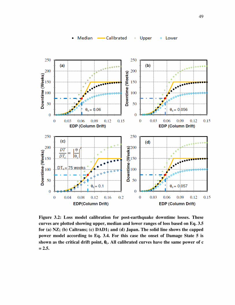
Table 3.1 is then used to multiply the vulnerability probability with expected

losses (consequences) to obtain probable losses for a given EDP. The sum of the product

of probability of drift and its expected outcome (Eq. (3.5)) is then calibrated using the

power curve with the upper and lower cutoffs. The model is calibrated for different

bridges located in California and New Zealand. For each type of bridge, the sum of

product of downtime losses from Table 3.1 and the lognormal distributed drift

corresponding to each damage state (Solberg et al. 2008; Sircar et al. 2009) is calculated

and a curve is generated. The median values thus obtained are curve fitted using power

curve with upper and lower cutoff as shown in Figure 3.2. It is observed from the results

that the exponent of calibrated downtime loss model, ‘c’, for bridges is 2.5 (Figure 3.2).

Similary, a relationship is established between EDP and downtime losses for buildings

using downtime loss data from Comerio (2000). The critical drift for buildings is

assumed as 0.06 (Kircher et al. 1997). For buildings, the downtime at critical drift

depends on floor area and the exponent ‘c’ decreases with increase in floor area (Figure

3.3). There are considerable epistemic uncertainties in these estimates due to contractual

variabilities and scope of work, this is discussed below.

3.5 Uncertainty and the Analysis of EADT

Using the calibrated downtime loss model along with hazard and structural

analysis, downtime loss estimation can be developed. Utilizing dispersion factors, in

conjunction with median coordinates, an expected value (mean) loss curve can be

developed. Expected annual downtime (EADT) may be estimated by simply calculating

the area under mean curve of the Figure 3.1(d) which can expressed as:

48

#$�Q = . �/���Q0000�� + ���1 �Q0000�1 + � 2 �34 � ≠ −1 (3.6)

where ( �/��, �Q0000��) and (�/�, �Q0000�), are the mean values of the primary downtime loss

curve coordinates.

The mean values of coordinates can be estimated using:

�/�� = �<�� = ���� �G���G�� ��� (3.7)

where �/�� and �<�� are mean and median value of the frequency at the onset of damage,

respectively. Note these are identical because the underlying distribution of damage

onset is assumed to be normal. Similarly using Eq. 3.1 in terms of mean parameters:

�Q0000�� = �Q0000��� = �/������="

(3.8)

in which:

�Q0000��� = �Q>��� exp (0.5CDEF ) (3.9)

where

�Q>��� = �Q>� �G���G� �� (3.10)

and

CDEF = CHEF + �F(CI�F + CIJF ) (3.11)

where �Q>� = median downtime at critical drift; CHE = epistemic uncertainty in downtime

loss estimation = 0.35; with CI� and CIJ being the aleotoric randomness dispersions in

structural capacity and demand, respectively.

49

Figure 3.2: Loss model calibration for post-earthquake downtime losses. These

curves are plotted showing upper, median and lower ranges of loss based on Eq. 3.5

for (a) NZ; (b) Caltrans; (c) DAD1; and (d) Japan. The solid line shows the capped

power model according to Eq. 3.4. For this case the onset of Damage State 5 is

shown as the critical drift point, θθθθc. All calibrated curves have the same power of c

= 2.5.

50

Figure 3.3: Downtime for given engineering demand parameter (column drift)

using data from Comerio (2000) for: (a) Large structural buildings with floor area

more than 80,000 square feet (c = 1.5); and (b) Small structural buildings with floor

area less than 80,000 square feet (c = 1.75). θθθθc = 0.06 is a typical complete damage

drift taken for buildings (Kircher et al. 1997).

51

The mean downtime loss at complete collapse or toppling is:

�Q0000� = �Q>� exp (0.5CHEF ) (3.12)

�/� = ���� = �Q0000��Q0000���=K" (3.13)

Values of these aleatoric and epistemic uncertainties are given in Table 3.2 along

with the associated dispersion factors.

3.6 Case Study for Bridges

The prototype of bridge for Caltrans, New Zealand and Japan is shown in Figure

3.4(a). The DAD design for California seismicity with same dimension as of Caltrans

bridge is shown in Figure 3.4(b). Four-step model for California seismicity is shown in

Figure 3.5 for non-seismic, Caltrans and DAD2 bridges whereas comparison of bridge

designs from New Zealand, Japan and DAD1 (designed for NZ seismicity) is shown in

Figure 3.6. The results of four-step model for various bridges are tabulate in Table 3.2

with mean and median parameters.

Result in Table 3.2 shows that EADT for non-seismically designed bridges is

2.11 days whereas for bridge designed using Caltrans specifications has only 6 hours of

expected annual downtime. Bridge designed using DAD technique in California

seismicity (DAD2) performs better than Caltrans design with only 3.6 hours as expected

annual downtime. Bridges designed to New Zealand specifications show more than 16.5

hours as downtime and DAD designed in NZ seismicity (DAD1) has only 5.5 hours as

expected annual downtime.

52

The prototype bridge is considered to see the relative importance of 3D losses

and compare bridge losses on monetary scale. The prototype bridge of five-spans 40 m

each and 15 m width is assumed to be constructed with a cost of $1,200/m2. The annual

average daily traffic (AADT) is assumed as 60,000 with occupancy of a vehicle as 1.2.

Based on U.S. Department of Transportation (2007) recommendations, the value of

statistical life is assumed as $ 6.0 million. The toll tax is assumed as the sum of amount

the bridge owner will lose as toll, the cost of extra miles traveled by the driver to reroute

and wear and tear to the rerouted route. It is conservatively assumed as $1.0 per vehicle

per pass. Result shows that Caltrans design saves more than $149,000 per year by just

adapting the ductile design and DAD design can save another $11,000 per year just by

improving the detailing of connections (Table 3.3). Table 3.3 shows 3D losses for

different prototype bridges in terms of total expected annual losses.

It is also of interest to have some insight as to the expected downtime for the two

commonly used earthquakes applied in design, specifically DBE and MCE (maximum

considered earthquake, 2% in 50 years). Table 3.4 shows the scenario losses for DBE

and MCE in California region based on different detailing. Table 3.5 uses these scenario

losses from Table 3.4 for prototype bridge and estimate losses in monetary terms.

Figure 3.7 represent the total expected annual losses in stacked column chart for

all these different prototype bridges and Figure 3.8 represent scenario event losses for

bridges in Caltrans seismicity showing individual Damage, Death and Downtime losses.

53

Figure 3.4: Five-span prototype bridge used in study. (a) Bridge piers studied by

Mander et al. (2007) and (b) DAD pier designed for California seismicity (DAD2).

(a)

(b)

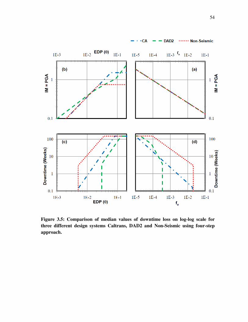
54

Figure 3.5: Comparison of median values of downtime loss on log-log scale for

three different design systems Caltrans, DAD2 and Non-Seismic using four-step

approach.

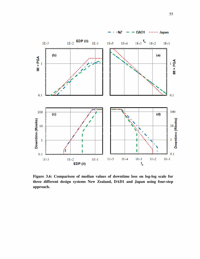
55

Figure 3.6: Comparison of median values of downtime loss on log-log scale for

three different design systems New Zealand, DAD1 and Japan using four-step

approach.

56

Table 3.2: Calculation of expected annual downtime (in Days) for different bridge

designs along with median and mean parameters.

Parameters Non-

Seismic CALTRANS DAD2 JAPAN NZ DAD1 Remarks

a)

IMDBE 0.4 0.4 0.4 0.4 0.4 0.4 Solberg et al.

(2008) fDBE 0.0021 0.0021 0.0021 0.0021 0.0021 0.0021

k 3.45 3.45 3.45 2.4 3 3

b) θθθθDBE 0.0115 0.0117 0.013 0.0115 0.0163 0.0165 IDA

Calibration b 1.25 1.25 2 1.23 1.27 1.69

c)

θθθθon 0.005 0.0053 0.03 0.0053 0.0062 0.03 Sircar et al.

(2009) θθθθc 0.025 0.0616 0.1 0.0566 0.0564 0.1

f 1 1 1 1 1 1

c 2 2.5 2.5 2.5 2.5 2.5 Calibrated

DTDBE 15.87 1.179 0.457 1.396 3.368 0.8294 Eq. 3.10

Me

dia

n P

ara

me

ters

d -0.725 -0.906 -1.449 -1.281 -1.058 -1.408 = b c / -k

DTU 150 150 150 150 150 150 Assigned

DTon 3 0.163 3.697 0.201 0.3 3.697 Eq. 3.4

fu 9.46E-05 9.97E-06 1.93E-05 5.5E-05 5.81E-05 5.24E-05 Eq. 3.3

fon 0.02092 0.01868 0.00035 0.0095 0.0206 0.0007 Eq. 3.7

fmid - - 8.14E-05 - - - Solberg et al.

(2008) DTmid - - 52.8 - - -

Me

an

Pa

ram

ete

rs

ββββRD 0.42 0.42 0.42 0.4 0.43 0.42 IDA Solberg et

al. (2008) ββββRC 0.2 0.2 0.2 0.2 0.2 0.2

ββββUS 0.25 0.25 0.25 0.25 0.25 0.25

ββββUL 0.35 0.35 0.35 0.35 0.35 0.35 Estimated

ββββRS 0.5281 0.5281 0.5281 0.5123 0.5361 0.5281 Calculated

ββββFon|θθθθ 0.552 0.552 0.345 0.390 0.472 0.355 = k/b*βRC

ββββTL 0.994 1.215 1.215 1.172 1.236 1.215 Eq. 3.11

DTDBE 26.01 2.465 0.956 2.77 7.23 1.73 Eq. 3.9

DTU 159.47 159.47 159.47 159.47 159.47 159.47 Eq. 3.12

fu 17.2E-05 2.10E-05 6.15E-05 8.9E-05 11.3E-05 8.47E-05 Eq. 3.13

DTon 4.92 0.34 12.75 0.40 0.645 7.73 Eq. 3.8

fon 0.0209 0.0187 0.0004 0.0095 0.0206 0.0007 Eq. 3.7

DTmid - - 110.38 - - -

Solberg et al.

(2008)

fmid - - 7.92E-05 - - -

don - - -1.449 - - -

du - - -0.725 - - -

EADT (days) 2.11 0.25 0.15 0.36 0.69 0.23 Eq. 3.6

57

Table 3.3: Comparative study of a prototype bridge showing total loss (Damage,

Death and Downtime) per year for different bridge designs.

Parameters Non

Seismic Caltrans DAD2 Japan NZ DAD1

EAL ($/million) 6,210 917 176 970 1,773 328

FAR 4.62 0.88 0.27 1.19 2.20 0.74

EADL 0.000405 7.72E-05 2.37E-05 0.000104 0.000193 6.49E-05

EADT 2.11 0.25 0.15 0.36 0.69 0.23

Damage Loss 22,356 3,301 634 3,492 6,383 1,181

Human Loss 22,664 4,317 1,325 5,838 10,792 3,630

Downtime Loss ($) 126,600 15,000 9,000 21,600 41,400 13,800

Total Loss ($)/year 171,620 22,618 10,958 30,930 58,575 18,611

% Cost of Bridge 4.77 0.63 0.30 0.86 1.63 0.52

Analysis Assumptions Length of bridge = 200m (five spans of 40m); Breath = 15m; Construction Cost = $1,200/m2 ; Total Construction Cost = $ 3.6 million Vehicle Speed = 100km/h; Vehicle Occupancy = 1.2 Annual Average Daily Traffic, AADT = 60,000 Value of a Statistical Life, VSL = $ 6 million Approach stopping distance =100m (for 100 km/h speed) Assumed equivalent toll tax for each passage = $ 1.0

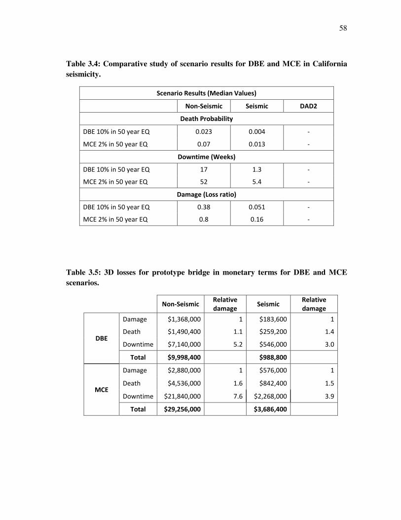
58

Table 3.4: Comparative study of scenario results for DBE and MCE in California

seismicity.

Scenario Results (Median Values)

Non-Seismic Seismic DAD2

Death Probability

DBE 10% in 50 year EQ 0.023 0.004 -

MCE 2% in 50 year EQ 0.07 0.013 -

Downtime (Weeks)

DBE 10% in 50 year EQ 17 1.3 -

MCE 2% in 50 year EQ 52 5.4 -

Damage (Loss ratio)

DBE 10% in 50 year EQ 0.38 0.051 -

MCE 2% in 50 year EQ 0.8 0.16 -

Table 3.5: 3D losses for prototype bridge in monetary terms for DBE and MCE

scenarios.

Non-Seismic

Relative

damage Seismic

Relative

damage

DBE

Damage $1,368,000 1 $183,600 1

Death $1,490,400 1.1 $259,200 1.4

Downtime $7,140,000 5.2 $546,000 3.0

Total $9,998,400 $988,800

MCE

Damage $2,880,000 1 $576,000 1

Death $4,536,000 1.6 $842,400 1.5

Downtime $21,840,000 7.6 $2,268,000 3.9

Total $29,256,000 $3,686,400

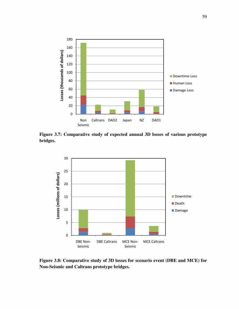
59

Figure 3.7: Comparative study of expected annual 3D losses of various prototype

bridges.

Figure 3.8: Comparative study of 3D losses for scenario event (DBE and MCE) for

Non-Seismic and Caltrans prototype bridges.

0

20

40

60

80

100

120

140

160

180

Non

Seismic

Caltrans DAD2 Japan NZ DAD1

Loss

es

(th

ou

san

ds

of

do

lla

rs)

Downtime Loss

Human Loss

Damage Loss

0

5

10

15

20

25

30

DBE Non-

Seismic

DBE Caltrans MCE Non-

Seismic

MCE Caltrans

Loss

es

(mil

lio

ns

of

do

lla

rs)

Downtime

Death

Damage

60

3.7 Discussion

Although the simple direct four-step probabilistic loss estimation framework

works well in estimating the 3D losses. The absolute accuracy may be quite dependent

on certain parameters and assumptions leaving the final results in doubt.

Notwithstanding this, for comparative purposes the results should remain consistent

amongst the different options considered. As it can be seen from the results, downtime

losses are the most significant for the cases investigated. Results shows that compared to

their historic non-seismic counterparts, modern ductile bridges designed in accordance

with contemporary seismic design specifications (e.g. Caltrans) have significantly less

total losses expected. Improved detailing using for example the emerging DAD armoring

details further improves the overall system performance. The cost for making any of

these improvement changes in the design is negligible, and therefore clearly worthwhile.

Also, when comparing the two DAD designs, DAD1 vs. DAD2, the latter is essentially

the same, but stronger – a clear benefit.

A sensitivity analysis was carried out to investigate the effects of key parameters

on downtime losses. The parameters were varied (one at a time) by 10% and

corresponding change in downtime losses measured (Figure 3.9). It is observed that the

calibrated loss model has least effect on the estimated downtime, as 10% variation in c

can affect less than 2% the estimated downtime but is most sensitive to the use

parameter, AADT and tax. Similarly, Figure 3.10 considers the swing analysis in total

expected annual losses for various parameters of prototype DAD2 bridge.

61

Figure 3.9: Swing analysis with variation of 10% of different parameters for

calculation of expected annual downtime losses for DAD1.

Figure 3.10: Swing analysis with variation of 10% of different parameters for

calculation of total expected annual losses for prototype DAD2 bridge.

-30 -20 -10 0 10 20 30

cθθ θθ

on

θθ θθcr

θθ θθ

DB

Eb

k

-10 -5 0 5 10

L O

ccu

pan

cy

V

T

oll T

ax A

AD

T

62

3.8 Section Closure

From the research presented in this section the following conclusions are drawn:

1. The four-step probabilistic rapid loss estimation framework can be easily applied

to estimate 3D losses and can be calibrated for different kinds of simple bridge

structures.

2. Downtime leads to the most significant losses which can totally overshadow the

other losses due to damage and death. Clearly, it is really important to consider

downtime losses for constructed facilities in public ownership as a significant

sector of society become affected when such facilities are out of commission.

Likewise, similar constructed facilities in private sector ownership are also

affected. Lack of business continuity due to significant downtime may affect

long term business viability.

3. The emerging DAD approach can also reduce losses both in overall EAL, but

perhaps more significantly losses under DBE and MCE can essentially be

eliminated with judicious design.

4. Ductile design reduces 3D losses significantly for smaller earthquakes and it fails

to perform in larger once. Although ductility clearly helps, there is also no

substitution for high strength.

63

4. SUMMARY, CONCLUSIONS AND RECOMMENDATIONS

4.1 Summary

It is important to communicate the risk to life facility downtime associated with

the physical damage to structures arising from natural hazards. A quantitative risk

assessment technique was used to examine the total losses due to earthquakes. This work

extended the four-step direct loss modeling developed by Mander and Sircar (2009).

That approach used a combination of fragility curves and loss functions used for

probabilistic risk assessment methodology to estimate expected annual loss for structure.

The four-step approach was subdivided into four distinct tasks ((a) Hazard analysis, (b)

Structural analysis, (c) Loss analysis and (d) Loss estimation) and was conducted for

damage, death and downtime (the 3D’s) for common class of highway bridges.

The expected annual loss was derived from all possible earthquakes after

accounting for the uncertainties in the response and modeling process. Empirically

calibrated models in the form of power curves that are capped with upper and lower

bounds were used to model death and downtime losses from the onset of damage until

toppling or collapse occurs.

The utility of the approach was investigated for the bridges in both California and

New Zealand regions for different design and detailing specifications. The results

indicated that death losses for bridges were generally greater than one and downtime

four times that of direct physical damage losses. It was also shown that the FAR for

DAD was much less than the risk exposure to a person sleeping whereas for non-

64

seismically designed structures, it was four and half times higher. DAD structures were

demonstrated to perform really well as compared to existing ductile systems with almost

same cost of design and construction. The model was demonstrated to be a useful tool in

comparing structures to both scenario losses and expected annual losses.

4.2 Conclusions

The following are the major conclusions from this study:

i. The four-step risk modeling approach is shown to be a comprehensive

stochastic model for estimating the 3D (death, downtime and damage) losses

due to earthquakes.

ii. Death losses due to earthquakes are slightly more than damage losses. The

FAR for non-seismic structure is 4.62; for seismic, it is 0.88 and for DAD it

is 0.27. This shows that non-seismic structures are 4.5 times more risky than

sleeping activity (FAR = 1.0). DAD structures are at least 70% less risky.

iii. The expected annual downtime loss (EADT) for all possible earthquake

scenarios is at least 2 days per year for non-seismic (non-ductile) structures,

whereas for their ductile seismic-resistant counterparts EADT = 0.25 days per

year. Such a value for the latter may seem insignificantly small. However, in

the context of a MCE (2% in 50 years) the picture is much darker: Non-

seismic and seismically designed structures are expected to be down for 52

and 5 weeks respectively.

iv. Losses can be further reduced or negated if DAD concepts are employed in

design and construction.

65

4.3 Recommendations for Further Work

This section outlines a few important areas in which further study is essential:

i. Experimental and practical investigations are required to verify the results

from the model.

ii. More detail and rigorous analysis is required to confirm the better response of

DAD types of structures in seismic hazards.

iii. To a greater extent, model needs more accurate and realistic relationship

between damages states and 3D losses. Practical regional studies should serve

this purpose where, the death loss should also depend on significance and

importance of the structure (like a school building), and downtime on floor

area of buildings.

iv. More detail study is required for estimating downtime cost of money as it

depends on the location and it varies from owner to user point of view. For

example, in case of bridges, a more detailed origin-destination network

analysis is needed for reliable results.

66

REFERENCES

Acton, J. P. (1976). “Measuring the monetary value of lifesaving programs.” Law and

Contemporary Problems, 40(4), 46-72.

Ajrab, J. J., Pekcan, G., and Mander, J. B. (2004). “Rocking wall-frame structures with

supplemental tendon systems.” Journal of Structural Engineering, 130(6), 895-

903.

Algermissen, S. T. (1972). A study of earthquake losses in the San Francisco Bay area,

Office of Emergency Preparedness and National Oceanic and Atmospheric

Administration, Washington, D.C.

Baker, J. W., and Cornell, C. A. (2008). “Uncertainty propagation in probabilistic

seismic loss estimation.” Structural Safety, 30(3), 236-252.

Basoz, N., and Mander, J. B. (1999). “Enhancement of the highway transportation

lifeline module in HAZUS.” National Institute of Building Sciences, 16(1), 31-

40.

Beck, J. L., Kiremidjian, A., Wilkie, S., Mason, A., Salmo, T., Goltz, J., Olsan, R.,

Workman, J., Irfanoglu, A., and Porter, K. A. (1999). “Decision support tools for

earthquake recovery of business.” CUREe-Kajima Phase III Project, Consortium

of Universities for Research in Earthquake Engineering, Richmond, CA.

67

Bradley, B. A., Dhakal, R. P., Cubrinovski, M., Mander, J. B., and MacRae, G. A.

(2007). “Improved seismic hazard model with application to probabilistic seismic

demand analysis.” Earthquake Engineering & Structural Dynamics, 36(14),

2211-2225.

Comerio, M. C. (2000). The economic benefits of disaster resistant university, Institute

of Urban and Regional Development, University of California, Berkeley, CA.

Comerio, M. C. (2006). “Estimating downtime in loss modeling.” Earthquake Spectra,

22(2), 349-365.

Cornell, C. A. (1968). “Engineering seismic risk analysis.” Bulletin of the Seismological

Society of America, 58(5), 1583-1606.

Cornell, C. A., Jalayer, F., Hamburger, R. O., and Foutch, D. A. (2002). “Probabilistic

basis for 2000 SAC federal emergency management agency steel moment frame

guidelines.” Journal of Structural Engineering, 128(4), 526-533.

Cornell, C. A., and Krawinkler, H. (2000). Progress and challenges in seismic

performance assessment, PEER Center News, University of California, Berkeley,

CA.

Dhakal, R. P., Khare, R. K., and Mander, J. B. (2006). “Economic payback of improved

detailing for concrete buildings with precast hollow-core floors.” Bulletin of the

New Zealand Society for Earthquake Engineering, 39(2), 106-119.

68

Dhakal, R. P., and Mander, J. B. (2006). “Financial risk assessment methodology for

natural hazards.” Bulletin of the New Zealand Society for Earthquake

Engineering, 39(2), 91-105.

Department of Homeland Security (DHS). (2009). National infrastructure protection

plan, National Institute of Building Science, Washington, D.C.

Dunster, H. J., and Vinck, W. (1979). “The assessment of risk-its value and limitations.”

Nuclear Engineering International, 15(3), 23-37.

Elms, D. G., and Mander, J. B. (1990). Locomotive engineer hazards: A quantitative risk

assessment study, Institution of Professional Engineers, Wellington, New

Zealand.

Garrick, B. J., and Christie, R. F. (2002). “Probabilistic risk assessment practices in the

USA for nuclear power plants.” Safety Science, 40(1-4), 177-201.

Gibson, S. B. (1976). “Risk criteria in hazard analysis.” Chemical Engineering Progress,

72(2), 59-62.

Goulet, C. A., Haselton, C. B., Mitrani-Reiser, J., Beck, J. L., Deierlein, G. G., Porter, K.

A., and Stewart, J. P. (2007). “Evaluation of the seismic performance of a code-

conforming reinforced-concrete frame building: From seismic hazard to collapse

safety and economic losses.” Earthquake Engineering & Structural Dynamics,

36(13), 1973-1997.

69

Griffiths, R. F. (1978). “Reactor accidents and the environment.” Atom, 266(2), 314-325.

Hamid, N. H., and Mander, J. B. (2006). “Damage avoidance design of warehouses

using precast hollow core walls system.” Engineering Structures, 9(1), 1-573.

HAZUS. (1997). Earthquake loss estimation methodology, Technical manual, developed

by the Federal Emergency Management Agency, Washington, D.C.

HAZUS. (2003). Multi-hazard loss estimation methodology earthquake model,

Technical manual, developed by the Federal Emergency Management Agency,

Washington, D.C.

Henley, J. E., and Kumamoto, H. (1992). Probabilistic risk assessment, IEEE Press,

New York, NY.

Jones-Lee, M. W. (1976). The value of life: An economic analysis, University of

Chicago Press, Chicago, IL.

Kennedy, R. P. (1999). “Risk based seismic design criteria.” Nuclear Engineering and

Design, 192(3), 117-135.

Kennedy, R. P., Cornell, C. A., Campbell, R. D., Kaplan, S., and Perla, H. F. (1980).

“Probabilistic seismic safety study of an existing nuclear power plant.” Nuclear

Engineering and Design, 59(2), 315-338.

Kennedy, R. P., and Ravindra, M. K. (1984). “Seismic fragilities for nuclear power plant

risk studies.” Nuclear Engineering and Design, 79(1), 47-68.

70

Kircher, C. A. (2003). “Earthquake loss estimation methods for welded steel moment-

frame buildings.” Earthquake Spectra, 19(2), 365-384.

Kircher, C. A., Nassar, A. A., Kustu, O., and Holmes, W. T. (1997). “Development of

building damage functions for earthquake loss estimation.” Earthquake Spectra,

13(4), 663-682.

Kletz, T. A. (1971). “Hazard analysis: A quantitative approach to safety.” Proc.,

Symposium of British Institution of Chemical Engineers, London, UK, 75-87.

Kletz, T. A. (1978). “Hazard analysis, its application to risks to the public at large.”

Reliability Engineering, 3(4), 325-338.

Kniesner, T. J., and Leeth, J. (1991). “Compensating wage differentials for fatal injury

risk in Australia, Japan and United States.” Journal of Risk and Uncertainty,

4(1), 75-90.

Kniesner, T. J., Viscusi, W. K., and Ziliak, J. P. (2009). “Policy relevant heterogeneity in

the value of statistical life: New evidence from panel data quantile regressions.”

Journal of Risk and Uncertainty, 40(1), 15-31.

Lawley, H. G. (1980). “Safety technology in the chemical industry: A problem in hazard

analysis with solution.” Reliability Engineering, 1(2), 89-113.

Lawley, H. G., and Kletz, T. A. (1975). “High-pressure trip systems for vessel

protection.” Chemical Engineering, 82(3), 81-93.

71

Lees, F. P. (1980). Loss prevention in the process industries, Loughborough University,

Leeds, England.

Linnerooth, J. (1979). “The value of human life: A review of the models.” Economic

Injury, 17(1), 52-74.

Mackie, K. R., Wong, J. M., and Stojadinovic, B. (2009). “Post-earthquake bridge repair

cost and repair time estimation methodology.” Earthquake Engineering &

Structural Dynamics, 39(3), 281-301.

Mander, J. B., and Basoz, N. (1999). “Seismic fragility theory for highway bridges:

Optimizing post-earthquake lifeline system reliability.” Proc., Fifth US

Conference on Lifeline Earthquake Engineering, Seattle, WA, 70-85.

Mander, J. B., and Cheng, C. T. (1997). Seismic resistance of bridge piers based on

damage avoidance design, National Center for Earthquake Engineering

Research, Buffalo, NY.

Mander, J. B., Dhakal, R. P., Mashiko, N., and Solberg, K. M. (2007). “Incremental

dynamic analysis applied to seismic financial risk assessment of bridges.”

Engineering Structures, 29(10), 2662-2672.

Mander, J. B., and Elms, D. G. (1994). “Quantitative risk assessment of large structural

systems.” Structural Safety & Reliability, 3(1), 1905-1912.

72

Mander, J., and Sircar, J. (2009). “Loss model for seismically damaged

structures.” Proc., 2009 Structures Congress, ASCE, Austin, TX, 1077-1086.

Miller, T. R. (2000). “Variations between countries in value if statistical life.” Journal of

Transport Economics and Policy, 34(2), 169-188.

National Institute of Building Sciences (NIBS). (1994). Assessment of state of the art

earthquake loss estimation methodologies, FEMA-249, Washington, D.C.

Porter, K. A., Beck, J. L., and Shaikhutdinov, R. (2004). “Simplified estimation of

economic seismic risk for buildings.” Earthquake Spectra, 20(4), 1239-1263.

Porter, K. A., Kiremidjian, A. S., and LeGrue, J. S. (2001). “Assembly-based

vulnerability of buildings and its use in performance evaluation.” Earthquake

Spectra, 17(2), 291-312.

Rhoads, S. E. (1978). “How much should we spend to save a life?” Public Interest,

51(51), 74-92.

Rice, D., and Cooper, B. S. (1967). “The economic value of life.” American Journal of

Public Health, 57(11), 1954-1966.

Shiono, K., Mubakami, H., Okada, S., and Ohta, Y. (1995). Lessons learned from

reconstruction following a disaster: Enhancement of regional seismic safety

attained after the 1976 Tangshan, China Earthquake, Japan Society of Civil

Engineers, Dotoku Gakkai, Japan.

73

Shome, N., and Cornell, C. A. (1999). Probabilistic seismic demand analysis of

nonlinear structures, RMS Program, Stanford University, Stanford, CA.

Sircar, J., Damnjanovic, I., Mander, J., and Aslan, Z. (2009). “Catastrophe bonds for

transportation assests: A feasibility analysis.” Journal of Transportation

Research Record, 2115(1), 12-19.

Solberg, K. M. (2007). Experimental and financial investigations into the further

development of damage avoidance design, University of Canterbury, Canterbury,

New Zealand.

Solberg, K. M., Dhakal, R. P., Mander, J. B., and Bradley, B. A. (2008). “Computational

and rapid expected annual loss estimation methodologies for structures.”

Earthquake Engineering & Structural Dynamics, 37(1), 81-101.

Stewart, M. G. (2009). “Risk-informed decision support for assessing the costs and

benefits of counter-terrorism protective measures for infrastructure.”

International Journal of Critical Infrastructure Protection, 2010(3), 29-40.

Thaler, R., and Rosen, S. (1976). The value of saving a life: Evidence from the labor

market, Household Production and Consumption, Columbia University Press,

New York.

U.S. Department of Transportation. (2007). Treatment of the economic value of a

statistical life in department analyses, Office of Assistant Secretary for

Transportation Policy, Washington, D.C.

74

Vamvatsikos, D., and Cornell, C. A. (2002). “Incremental dynamics analysis.”

Earthquake Engineering & Structural Dynamics, 31(3), 491-514.

Viscusi, W. K. (1978). “Labour market valuations of life and limb: Empirical evidence

and policy implications.” Public Policy, 26(3), 359-386.

Whitman, R. V., Anagnos, T., Kircher, C. A., Lagorio, H. J., Lawson, R. S., and

Schneider, P. (1997). “Development of a national earthquake loss estimation

methodology.” Earthquake Spectra, 13(4), 643-661.

75

VITA

Sandeep Ghorawat received his Bachelor of Technology degree from the Indian

Institute of Technology Guwahati, Assam, India in May of 2008. He entered the

structural engineering program at Texas A&M University in August 2008 and received

his Master of Science degree in May 2011.

Mr. Ghorawat may be reached at CE/TTI, Texas A&M University, 3136 TAMU,

College Station, TX 77843-3136, USA. His email is ghorawatiit04@gmail.com.