rashad cassim - uct faculty of humanities · the measurement of trade creation and diversion is...

D P R U WORKING PAPERS

The Determinants of Intra-Regional Trade in Southern Africa with Specific Reference

to South African and the Rest of the Region

Rashad Cassim

No 01/51 June 2001 ISBN: 0-7992-2057-4 Development Policy Research Unit

University of Cape Town

Abstract

The paper puts forward a case for more attention to be paid to fundamental structural factors that will determine the scope and success of any regional integration initiative in the Southern African Development Community (SADC). The paper provides a review of current estimates of trade potential in the region and contrasts this with the author's own estimates of intra-regional trade. A gravity model is used. The model examines how the reduction of trade transaction costs, the level of development and the size of an economy influences trade potential amongst countries. A major finding is that fundamental structural and economic factors such as the transaction costs of trading, the growth paths of economies and changes in per capita income should be the focus of regional integration rather than trade policy in its own right. The empirical results show that intra-regional trade in SADC is not low by international standards. When compared to regions such as the Southern African Customs Union (SACU) or Mercosur, actual South African exports are higher than estimated potential exports. However, the model indicates low trade volumes for combinations of countries in the SADC region. In particular, there is increasing scope for non-SACU countries to increase their exports to South Africa.

These arguments have to be seen in the context of the impending Free Trade Agreement (FTA) in the SADC region. There is no question about the fact that an FTA will enhance the prospects for increasing intra-regional trade. However, it is important not to exaggerate the impact of a regional agreement. In other words, there is no substitute for national economic policies that are conducive to growth.

Table of Contents

List of Tables

1. Introduction ............................................................................................................................................... 1

2. Review of Projections of Trade Potential In SADC.............................................................................. 1

3. The Determinants of Trade : The Gravity Model................................................................................. 6

4. The Model: Estimating Direction of Trade with Single Country Variables ....................................... 7

5. Future Trade Potential............................................................................................................................10

6. Implications of the Modelling Results..................................................................................................13

7. Conclusion...............................................................................................................................................15

Appendix 1...................................................................................................................................................17

Appendix 2...................................................................................................................................................20

Appendix 3...................................................................................................................................................21

Reference......................................................................................................................................................22

Table 1: Actual and Potential SADC 7 Exports to SACU, 1995 Millions of dollars............................. 2

Table 2: Results of Evans Model with Long-Run Armington Elasticities................................................ 4

Table 3: SADC Simulation of a Free Trade Agreement ........................................................................... 6

Table 4 : Model Single Country Variables: World Sample...................................................................... 8

Table 5: Actual, Potential and Projected Trade Flows based on SACU Control Group, Value in $1 million ................................................................................................................................................11

Table 6: Income Catch-up: Simulated Growth in GDP of SADC Countries ................................ ......13

D P R U W o r k i n g P a p e r N o . 0 1 / 5 1 R a s h a d C a s s i m

22

1. Introduction

Trade integration has become a central focus of policy-makers throughout Southern Africa. Although the appeal for increasing trade in the region may seem plausible, there are strictly speaking no well-grounded economic reasons why trade, in its own right, should be an obsession. More important is the need to explore the welfare of the region, and this may not be achievable by increasing trade.

There are, to date, very few studies in Southern Africa that give clear reasons why we should increase trade, the likely costs and benefits of increasing regional trade, and the form (intra-industry, inter-industry or intra-firm) that an increase in trade is likely to take. Will the growth in intra-regional trade be trade distorting? In other words, will growth in trade be induced more by trade diversion than by trade creation? One of the major indicators of successful integration is for member countries to generate increasing intra-regional trade by reducing the cost to trading in most cases through tariff reduction. Naturally, such trade has to be welfare enhancing and not driven by trade diversion.

One of the important points of departures for any trade study in the region is to begin with a basic analysis of trade creation and trade diversion. However, there are two essential reasons why the measurement of trade creation and diversion is difficult in the Southern African Development Community SADC) context. Firstly, it has been persistently pointed out that one of the greatest difficulties in measuring intra-regional trade in developing areas, such as Southern Africa, is the paucity of reliable trade data. A systematic product-by-product level data set also does not exist. Moreover, a large part of the trade is informal and goes unrecorded, which severely limits the usefulness of official statistics. The second problem stems from the complex hybrid of differential tariff structures, tariff equivalents and exemptions. Hence, this working paper abstracts from these issues and look at some of the fundamental structural factors influencing regional integration.

2. Review of Projections of Trade Potential In SADC

The SADC region consists of countries that are rather small in size and differ remarkably in levels of development. The important question to consider is does size and asymmetry in the level of development bias the prospects for integration? Does regional integration matter for economic growth? Specifically, can regional integration act as an impetus to growth or does low (and often divergent) growth influence the prospects for integration? This is an important issue because growth in the Southern Africa region is, by and large, low and highly variable amongst countries with signs of growing dispersion. The SADC region is typical of many developing regions showing high extra-regional trade intensities but low intra-regional trade biases. Moreover, the high trade intensity is a reflection of high levels of extra-regional trade with minimal growth in intra-regional trade. Noting these structural limitations, what is the potential for trade to grow in the short-, medium- and long-term?

This paper attempts to look at the potential for trade integration in the context of both the structural factors and growth behaviour of the region. A cross-section econometric gravity model is used to look not only at the potential for trade but also the main determinants of trade in the context of trade behaviour in other comparable regions.

A limited number of studies have emerged in the last few years looking at trade potential in the region. Two notable ones are reviewed here. The first relies on using fairly uncomplicated techniques and the second relies on using an elaborate partial equilibrium model.

T h e d e t e r m i n a n t s o f i n t r a - r e g i o n a l t r a d e i n S o u t h e r n A f r i c a

33

Specific trade potential between South Africa and the rest of the region, in a post-apartheid, post-sanctions era has received much attention. Various studies have emerged to project what the potential for trade is and in which likely products. There is general consensus that there is considerable potential.

One study shows that there is considerable potential for the non-Southern African Customs Union (SACU) countries to switch supply from third countries to South Africa. This implies that South Africa actually exports many of the products that the rest of Sub-Saharan Africa (SSA) imports from northern countries (but not from South Africa). These assumptions are derived from looking at potential trade, which is defined as the value of imports currently coming from the rest of the world for which at least one SSA country is making significant exports to the rest of the world (ADB, 1993). Using the same methodology, Mansoor et al (1993) show that potential intra-regional trade for SSA as a whole was $4.5 billion, 16 percent of the regions total exports for the year.

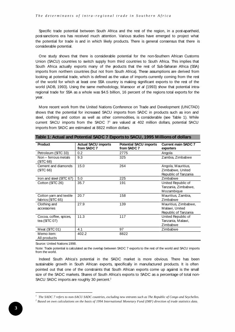
More recent work from the United Nations Conference on Trade and Development (UNCTAD) shows that the potential for increased SACU imports from SADC in products such as iron and steel, clothing and cotton as well as other commodities, is considerable (see Table 1). While current SACU imports from the SADC 71 are valued at 402 million dollars, potential SACU imports from SADC are estimated at 8822 million dollars.

Table 1: Actual and Potential SADC 7 Exports to SACU, 1995 Millions of dollars

Product Actual SACU imports from SADC 7

Potential SACU imports from SADC 7

Current main SADC 7 exporters

Petroleum (SITC 33) 0.2 2775 Angola Non – ferrous metals (SITC 68)

9.3 325 Zambia, Zimbabwe

Cement and diamonds (SITC 66)

15.0 264 Angola, Mauritius, Zimbabwe, United Republic of Tanzania

Iron and steel (SITC 67) 5.0 225 Zimbabwe Cotton (SITC 26) 35.7 191 United Republic of

Tanzania, Zimbabwe, Mozambique

Cotton yarn and textile fabrics (SITC 65)

20.7 158 Mauritius, Zambia, Zimbabwe

Clothing and accessories

27.9 139 Mauritius, Zimbabwe, Malawi, United Republic of Tanzania

Cocoa, coffee, spices, tea (SITC 07)

11.3 117 United Republic of Tanzania, Malawi, Zimbabwe

Meat (SITC 01) 4.1 97 Zimbabwe Memo item: All products

402.2 8822

Source: United Nations 1998. Note: Trade potential is calculated as the overlap between SADC 7 exports to the rest of the world and SACU imports from the world.

Indeed South Africa’s potential in the SADC market is more obvious. There has been sustainable growth in South African exports, specifically in manufactured products. It is often pointed out that one of the constraints that South African exports come up against is the small size of the SADC markets. Shares of South Africa’s exports to SADC as a percentage of total non-SACU SADC imports are roughly 30 percent.2

1 The SADC 7 refers to non-SACU SADC countries, excluding new entrants such as The Republic of Congo and Seychelles. 2 Based on own calculations on the basis of 1994 International Monetary Fund (IMF) direction of trade statistics data.


44

This analysis identifies the overlap of those products exported by SADC countries to the rest of the world while simultaneously imported by SACU from the rest of the world. It provides a useful general map of the trade potential between two regions since it examines trade potential rather than actual trade, focusing on the potential for SADC (excluding Mauritius) countries to export to SACU. Products with growth potential are those that SADC exports in large amounts to the rest of the world while SACU imports them in large amounts from the rest of the world.

These results are quite revealing but it is important to take cognisance of the fact that this methodology is crude and at best provides some pointers as to potential areas of complementarities. What is naturally needed is a closer analysis of the actual products, whether they are good substitutes and how competitive they are. The main weakness of this methodology is that it implicitly assumes that all potential trade is realisable and that the very definition of unexploited potential trade implies that the expected or attainable value of intra-product trade is zero. Moreover, trade potential identified in this way can only be a rough estimate because it is based on actual trade flows rather than on their determinants. Therefore supply capabilities in the potential exporting countries and market access conditions in potential importing countries also have to be taken into account (UNCTAD 1998: 204).

However, an important message emanating from these studies is that there is greater trade complementarity in Southern Africa than was previously believed. This is based on the fact that potential trade is higher than observed or official trade. An assessment of trade potential in SADC can be approached from various levels of sophistication. The most basic methodology was used above showing potential for greater intra-regional trade. As was noted, this methodology is somewhat crude and relies on too many assumptions. The following section reviews more sophisticated attempts to look, not only at trade potential, but other economic variables such as output and employment.

Evans (1997) develops a model that looks at the impact of a FTA in SADC on the economies of member countries. Evans goes beyond trade to look at employment and output.3 The model also shows the likely impact on government revenue due to losses of income from import duties. The multi-country partial equilibrium approach is similar in structure to a Computable General Equilibrium (CGE) model. It is lack of data that precluded the use of a region-wide CGE model.

The structure of the model is such that supply is determined by the so-called Armington4 rules for imports and domestic production. Imports and domestic production are regarded as imperfect substitutes and combined according to cost minimisation principles captured by functional relationships resembling the constant elasticity of substitution (CES) production function. Armington rules are also used to determine imports by source from SADC or the rest of the world. Demand is determined by price, exogenous income and exports from the rest of the world.

What the model attempts to do is to estimate the impact of a free trade agreement (FTA) on member countries. It does this under two scenarios. In the first scenario, it assumes a reduction in tariffs while everything else remains constant. In the second scenario, it assumes that the FTA is concluded with a 3 percent growth in the regions aggregate income5. There are minor differences in the results from the two scenarios but the conclusions are broadly the same. These are as follows:

3 I do not discuss the employment and output results from Evans as it is not of immediate concern except to acknowledge the welfare implications of measuring the impact of integration on trade include employment and output. 4 The Armington Assumption named after Paul Armington’s (1969) work involves a particular specification where products are considered imperfect substitutes. These products are simply differentiated by country of origin. 5 Evans also introduces Rest of World (ROW) effects but for my purposes I limit my discussion and results to SADC effects.


55

• The effect that the FTA has on total demand is low.

• The effect it has on imports into the SADC region as a whole is marginal since under a FTA the external tariff rates of countries remain the same or if these are reduced they are in keeping with World Trade Organisation (WTO) commitments.

• The overall impact of the FTA on employment is low although there may be specific sectors in the respective countries that may suffer.

• The FTA is likely to lead to trade creation of around 20 percent.

• A decline in revenue for some economies, which is somewhat predictable if tariffs come down.

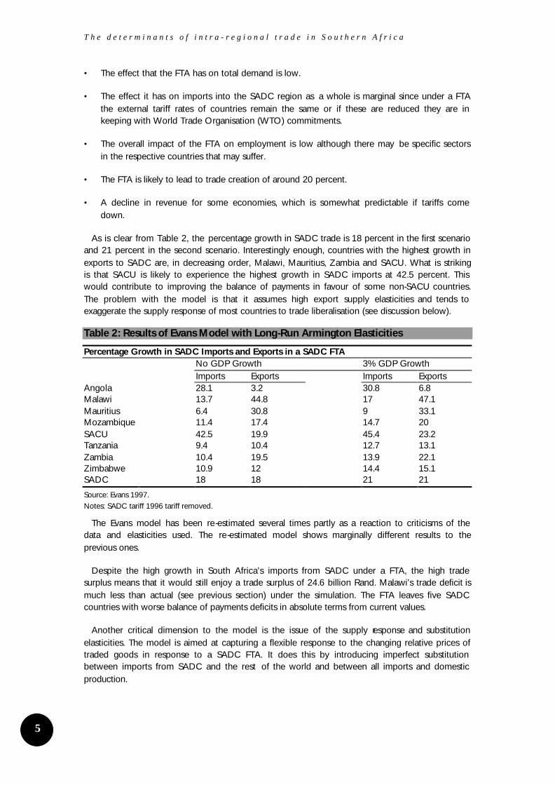
As is clear from Table 2, the percentage growth in SADC trade is 18 percent in the first scenario and 21 percent in the second scenario. Interestingly enough, countries with the highest growth in exports to SADC are, in decreasing order, Malawi, Mauritius, Zambia and SACU. What is striking is that SACU is likely to experience the highest growth in SADC imports at 42.5 percent. This would contribute to improving the balance of payments in favour of some non-SACU countries. The problem with the model is that it assumes high export supply elasticities and tends to exaggerate the supply response of most countries to trade liberalisation (see discussion below).

Table 2: Results of Evans Model with Long-Run Armington Elasticities

Percentage Growth in SADC Imports and Exports in a SADC FTA No GDP Growth 3% GDP Growth Imports Exports Imports Exports Angola 28.1 3.2 30.8 6.8 Malawi 13.7 44.8 17 47.1 Mauritius 6.4 30.8 9 33.1 Mozambique 11.4 17.4 14.7 20 SACU 42.5 19.9 45.4 23.2 Tanzania 9.4 10.4 12.7 13.1 Zambia 10.4 19.5 13.9 22.1 Zimbabwe 10.9 12 14.4 SADC 18 18 21

15.1 21

Source: Evans 1997. Notes: SADC tariff 1996 tariff removed.

The Evans model has been re-estimated several times partly as a reaction to criticisms of the data and elasticities used. The re-estimated model shows marginally different results to the previous ones.

Despite the high growth in South Africa’s imports from SADC under a FTA, the high trade surplus means that it would still enjoy a trade surplus of 24.6 billion Rand. Malawi’s trade deficit is much less than actual (see previous section) under the simulation. The FTA leaves five SADC countries with worse balance of payments deficits in absolute terms from current values.

Another critical dimension to the model is the issue of the supply response and substitution elasticities. The model is aimed at capturing a flexible response to the changing relative prices of traded goods in response to a SADC FTA. It does this by introducing imperfect substitution between imports from SADC and the rest of the world and between all imports and domestic production.


66

The model assumes perfectly elastic supply functions within each industry. In other words, a one percent increase in demand will automatically result in a one percent increase in supply. It also uses standard elasticities to estimate substitution effects or to determine how readily firms in one country will substitute their imports from a trading partner for domestic production. The choice of the elasticities requires more attention as this can critically influence the model results.

The model assumed a greater than unitary elasticity of substitution between domestic demand and foreign demand for consumer goods and lower elasticities for intermediate and capital goods. Domestic production and substitutable imports have an elasticity of 2,5. Exceptions are for the intermediate and the capital goods sectors where imports from domestic production are substitutable with the elasticity of 0,5. Imports from the two sources, that is, SADC and the rest of the world have an elasticity of 2,5. The degree of substitutability is not only applied in all sectors but also across sectors. The model also assumes infinite supply elasticities - this implies that there is excess capacity.

The important question is how do these assumed elasticties influence the results of the model. Cattaneo (1998: 224) questions the elasticity assumptions of the model arguing that there is no real basis for some of the assumptions. Cattaneo argues that in the consumer goods sectors, excess capacity assumptions, the assumptions of equal elasticity’s of substitution between imports from SADC and the ROW and between imports and domestic production tend to exaggerate the likely trade creation effects of a SADC FTA.

Based on the logic of the model, in consumer goods sectors, the removal of intra-SADC tariffs should result in an increase in imports from SADC, a fall in import competing production and a fall in imports from the ROW. Given the assumption of equal substitutability between imports from the two sources and imports and domestic production, it follows that for sectors in which the initial level of import-competing production exceeds imports from the ROW, trade creation will outweigh trade diversion.

In intermediate capital goods, imports are complements to domestic production, so that import competing production increases when a FTA is formed. However, these sectors still exhibit trade creation effects since there is still some substitution of imports for domestic production, although the effect is weak. The substitution effect between Msi (direction of change in imports from SADC) and Mri (direction of change in imports from the rest of the world) is, however, as strong as before so that in these sectors, trade diversion is likely to outweigh trade creation (Cattaneo 1998: 214). Cattaneo’s basic conclusion is that the choice of elasticities leads to an over estimation of the effects of trade creation. For sectors operating at full capacity the supply response is also likely to be exaggerated.

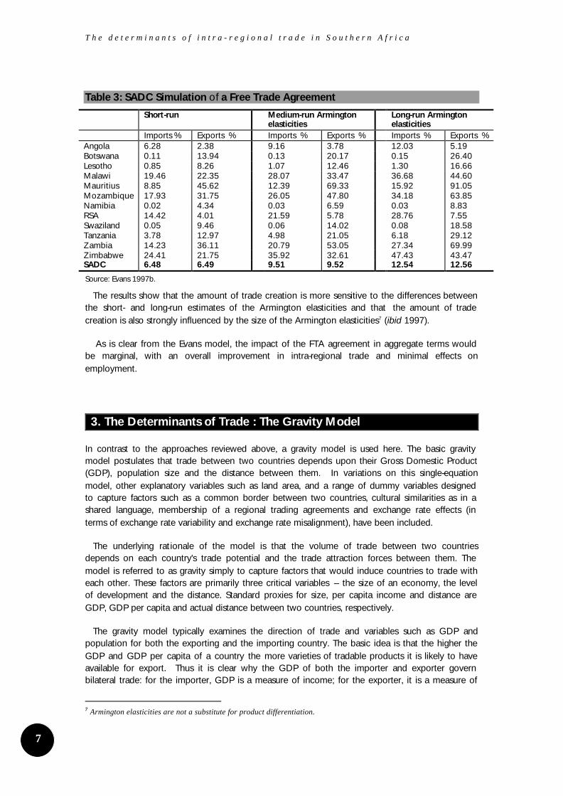
Evans (1997b), in a subsequent paper, revised the estimates and performed simulations with short-run, medium-run and long-run effects.6 The results are shown in Table 3 and as we can see total intra-regional trade is presumed to grow at 6.5 percent, 9.5 percent and 12.5 percent respectively.

6 Originally, the Armington elasticities were estimated for the Industrial Development Corporation (IDC) for their economy wide CGE model for the RSA. The basic estimates are intended to reflect short-run changes in relative prices and they have been extended to cover all SADC. The short run Armington elasticities were increased by 50 percent to arrive at medium-run elasticities and by 100 percent to arrive at long-run elasticities.


77

Table 3: SADC Simulation of a Free Trade Agreement

Short-run Medium-run Armington elasticities

Long-run Armington elasticities

Imports % Exports % Imports % Exports % Imports % Exports % Angola 6.28 2.38 9.16 3.78 12.03 5.19 Botswana 0.11 13.94 0.13 20.17 0.15 26.40 Lesotho 0.85 8.26 1.07 12.46 1.30 16.66 Malawi 19.46 22.35 28.07 33.47 36.68 44.60 Mauritius 8.85 45.62 12.39 69.33 15.92 91.05 Mozambique 17.93 31.75 26.05 47.80 34.18 63.85 Namibia 0.02 4.34 0.03 6.59 0.03 8.83 RSA 14.42 4.01 21.59 5.78 28.76 7.55 Swaziland 0.05 9.46 0.06 14.02 0.08 18.58 Tanzania 3.78 12.97 4.98 21.05 6.18 29.12 Zambia 14.23 36.11 20.79 53.05 27.34 69.99 Zimbabwe 24.41 21.75 35.92 32.61 47.43 43.47 SADC 6.48 6.49 9.51 9.52 12.54 12.56

Source: Evans 1997b.

The results show that the amount of trade creation is more sensitive to the differences between the short- and long-run estimates of the Armington elasticities and that the amount of trade creation is also strongly influenced by the size of the Armington elasticities7 (ibid 1997).

As is clear from the Evans model, the impact of the FTA agreement in aggregate terms would be marginal, with an overall improvement in intra-regional trade and minimal effects on employment.

3. The Determinants of Trade : The Gravity Model

In contrast to the approaches reviewed above, a gravity model is used here. The basic gravity model postulates that trade between two countries depends upon their Gross Domestic Product (GDP), population size and the distance between them. In variations on this single-equation model, other explanatory variables such as land area, and a range of dummy variables designed to capture factors such as a common border between two countries, cultural similarities as in a shared language, membership of a regional trading agreements and exchange rate effects (in terms of exchange rate variability and exchange rate misalignment), have been included.

The underlying rationale of the model is that the volume of trade between two countries depends on each country's trade potential and the trade attraction forces between them. The model is referred to as gravity simply to capture factors that would induce countries to trade with each other. These factors are primarily three critical variables – the size of an economy, the level of development and the distance. Standard proxies for size, per capita income and distance are GDP, GDP per capita and actual distance between two countries, respectively.

The gravity model typically examines the direction of trade and variables such as GDP and population for both the exporting and the importing country. The basic idea is that the higher the GDP and GDP per capita of a country the more varieties of tradable products it is likely to have available for export. Thus it is clear why the GDP of both the importer and exporter govern bilateral trade: for the importer, GDP is a measure of income; for the exporter, it is a measure of

7 Armington elasticities are not a substitute for product differentiation.


88

output8. The final step is to assume that the price that importers face for any given variety of exported products rises with the costs of conducting trade internationally (Baldwin 1994).

In terms of the logic of the model, distance will be inversely related to the volume of bilateral trade. Distance is used as the proxy variable for resistance to trade, which is composed of transport costs, commercial policy and imperfect information regarding export opportunities all of which may tend to become more meaningful with increased distance between countries. Thus the distance coefficient is meant to have a negative value (Markheim 1994:104-5).

Geographic size of the countries will be also inversely related to bilateral trade; the reasoning being that the larger economies trade proportionately less (not absolutely less). Exchange rate variability and exchange rate over-valuation are also expected to be inversely related to bilateral trade flows.

It is important to emphasise that the model is a generalised long-run structural model that aims to examine trade behaviour under certain conditions outlined above. The main attraction is that it relies on cross-country comparisons to develop a norm against which trade potential is measured in the SADC region.

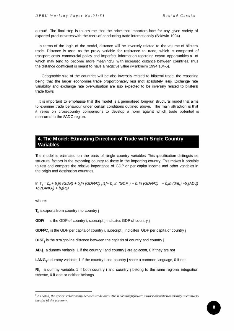
4. The Model: Estimating Direction of Trade with Single Country Variables

The model is estimated on the basis of single country variables. This specification distinguishes structural factors in the exporting country to those in the importing country. This makes it possible to test and compare the relative importance of GDP or per capita income and other variables in the origin and destination countries.

ln Tij = b0 + b1ln (GDPI) + b2ln (GDPPCi) [I1]+ b3 ln (GDPj ) + b4 ln (GDPPCj) + b5ln (distij) +b6(ADJij) +b7(LANGij) + b8(RIij)

where:

Tij is exports from country i to country j

GDPi is the GDP of country i, subscript j indicates GDP of country j

GDPPC i is the GDP per capita of country i, subscript j indicates GDP per capita of country j

DISTij is the straight-line distance between the capitals of country and country j

ADJij a dummy variable, 1 if the country i and country j are adjacent, 0 if they are not

LANGij a dummy variable, 1 if the country i and country j share a common language, 0 if not

RIij a dummy variable, 1 if both country i and country j belong to the same regional integration scheme, 0 if one or neither belongs

8 As noted, the apriori relationship between trade and GDP is not straightforward as trade orientation or intensity is sensitive to the size of the economy.


99

See Appendix 1 for discussion of variables.

All the traditional gravity variables are significant in explaining bilateral trade flows here. Income levels of the importing and exporting countries both have the expected positive sign, the contribution of the exporting country’s GDP is however slightly larger than that of the importing country - indicating that GDP, as the ability to export, is slightly more important here.

Table 4 : Model Single Country Variables: World Sample

Variable a. All Variables

b. Selected Variables

c. Selected Variables, with pop variables replaced by per capita income

Constant -11.141 -9.123 -8.5764 Log(GDPI) 1.0323* 0.9874* 1.1698* Log(GDPj) 0.69622* 0.6492* 1.0723* Log(disij) -0.44025* - 0.4889* -0.99759* ADJ 0.82052* - 0.9304* -0.70848E-01 Lang 0.70147* 0.5703* 0.64507* SADC 0.65683* Mer -0.15335E-02 Asean 0.72792* COMESA 0.32279 0.19290 -0.70193E-02 ISL 0.27695E-02 0.1748 0.45309E-03 Log(POP i) 0.12532* 0.21301* -0.15931* Log(POP j) -0.45849* -038615* -0.60060* Log(AREAI) -0.23424* -0.26797* -0.19707* Log(AREAj) -0.23827* -0.25874* -0.47188*

Note: Significance at the 5% confidence interval.

The distance variable has the right sign in the sense that increased trade is negatively correlated with distance. An interactive dummy was used as an indication that this variable may hide the fact that the transaction costs of trading in Africa in respect of distance are far higher than the world average. The interactive dummy was calculated as 1 for distance between two countries in Africa and 0 for distance anywhere else. This was multiplied by the actual distance used. However, the dummy was not significant.

The language and the adjacency variables are also highly robust. Language is significant and has a relatively large coefficient (0.7), which shows that countries with a similar language have the probability of trading more with each other. The language dummy essentially indicates how colonial ties influence the magnitude of trade between pairs of countries. However, this is more relevant to the north versus south divide – where Anglophone countries in Africa are likely to trade more with the UK than France. This opposite is true for Francophone countries.

Similarly, adjacency is significant with a high coefficient. In other words, the closer the countries, the more likely they are to trade with each other. However, if there is no complementary between two adjacent economies, then there is no intuitive reason why the adjacency coefficient should be positive.

The population variables are utilised as a proxy for market size. In Table 4 the population of the exporting country has a positive sign while the population of the importing country has the expected negative sign. This is contrary to expectations. The problem with the population variable is that larger economies with extreme population sizes such as India, China and to some extent the USA would be more autarkic than smaller economies such as Botswana or Lesotho. This is compounded by trade policy distortions where small populations may be less autarkic but more inward-looking. In other words, small non-diversified economies trade more of their output than


1010

larger diversified economies, purely because of the constraints of size, but may still have protected trade policies. Then, there are a series of middle-sized countries that are not as sensitive to a relationship between the population and openness. All these factors can easily distort the population variable and the sign of the coefficient in the estimation.

Markheim (1994:105) argues that more populous countries are assumed to have greater endowment of resources thereby allowing broad productive activities that in turn satisfy a greater proportion of domestic demand, whereas small countries tend to specialise in production and are more reliant on imports. Hence the smaller the population of the exporting countries the greater the likelihood of trade relative to its total income. From this angle, the signs of the coefficients are intuitive. However, at another level, the negative coefficient on the population of the importing country may be contrary to expectations – since a large importing country should promote trade as a larger population facilitates the division of labour and a variety of production lines that consequently provide opportunities for foreign goods to be incorporated into the production process.

Area, for both exporting and importing country, has the expected negative sign, indicating that larger countries are less likely to trade than smaller ones. Although the coefficients are not very large, they are significant. Economic size, on the other hand, as measured by GDP, is more sensitive to trade flows than geographic size.

The COMESA dummy is insignificant while the SADC dummy shows significance. This implies that the existence of SADC has a trade creating impact on the region. Intuitively, intra-regional trade, in SADC has increased marginally in the last decade. Its share, however, remains small relative to the extra-regional orientation of these countries.

Table 4, sets up three different equations. The first two (a and b) are very similar with the aim of testing the sensitivity of the results, for the main gravity variable parameters, for the inclusion of specific dummy variables. Column 4c is also a sensitivity test, but focuses on the impact of replacing one of the main variables, population with that of per capita income. The results change slightly. This is counter-intuitive in the sense that if log (GDP) is included, the results should be identical whether population or log (GDP/POP) is used. The different results may be explained by the fact that the per capita income is the GNP/per capita figure, which may be different from the GDP/per capita.

Some experimentation was carried out, specifically to test the relative sensitivities, or impact, of two interchangeable variables, namely per capita income and population. The model in Table 4 was re-estimated with GNP/per capita instead of the population. These results are presented in the last column of Table 4. It is interesting to note that when using per capita income, the coefficient of the exporting country is positive compared to the coefficient of population of the exporting country that is a negative. One reason is that in many countries, specifically in the developing world there is a more direct inverse link between large populations and market power. What is more reliable is the per capita income rather than the size of the population.

The model here attempts to look at how the exclusion of dummy variables influence, or bias the main explanatory variables. Interestingly, the exclusion of certain dummies in the second column does not make a significant difference to the coefficients, except for a slight reduction in the GDP coefficient and a slight increase in the distance variable. What is even more striking, however, is that the coefficient of the distance variable doubles when the equation is estimated without the dummies but instead uses per capita income rather than population.

An important message to take from this exercise is that the magnitudes of coefficients, as opposed to the level of significance or the signs of the coefficients, are sensitive to sample selection or the interchangeability of similar proxies. What remains consistent through all


1111

sensitivity exercises is the importance of some coefficients relative to others. For example, the coefficient of the GDP of the exporting country in models a to c has a different magnitude in every case but always remains the highest co-efficient. This signifies the enduring importance of the growth or the size of a country to export potential.

5. Future Trade Potential

Although the gravity model is not dynamic, one is able to derive ‘dynamic like’ results. By replacing the estimated set of coefficients with a set reflecting a plausible future state of affairs, one is simulating a potential trade scenario. This is done by using an appropriate non-SADC sample of countries and inserting the derived coefficients into the predictive equation consisting of Southern African country trade pairs. In general, the coefficients are calculated by inserting the main variables into the equation, which are then calculated and added in order to give potential or theoretical trade.

It was emphasised previously that the gravity model can be used both to decompose ex post the impact of integration on trade and to determine ex ante how different trading conditions, not necessarily a FTA, will influence future trade patterns. A major contribution of this paper is to focus on the latter. The key issue examined here is whether intra-regional SADC trade is low, high or normal. To determine this, a comparator region is used as a benchmark. If it is low, will SADC trade increase to normal levels and if so why? Put differently, what would intra-regional trade in Southern Africa be under different circumstances?

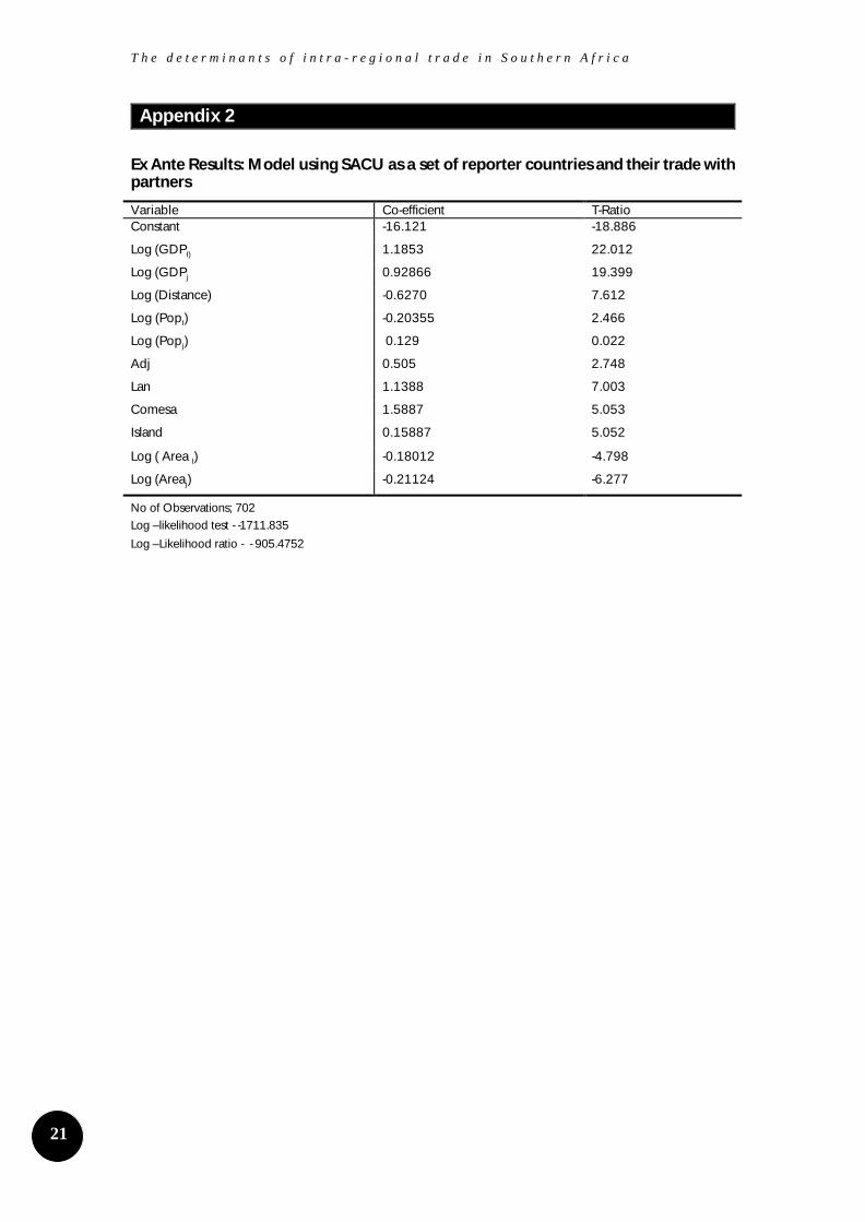
The coefficients of the base estimation using the SACU control group are shown in Appendix 2. What is important about the control group is that a dummy capturing the group, such as SACU, is excluded from the model simply because the aim is not to test the impact of SACU on trade but to structure a sample that characterises intra-SACU trade relative to SACU countries trade with other partners outside of the Customs Union (CU). Hence SACU is the reporting country in this sample and the rest of the trade combinations consist of their trading partners.

SACU is a very relevant and appropriate experiment. It has existed for a long time and has been one of the few, if not the only success story of market integration in Africa. Intra-regional trade is higher than that of the European Union (EU) and the economies in the region have converged considerably over the years. It is in a sense, a 'best case' microcosm of SADC in the future.

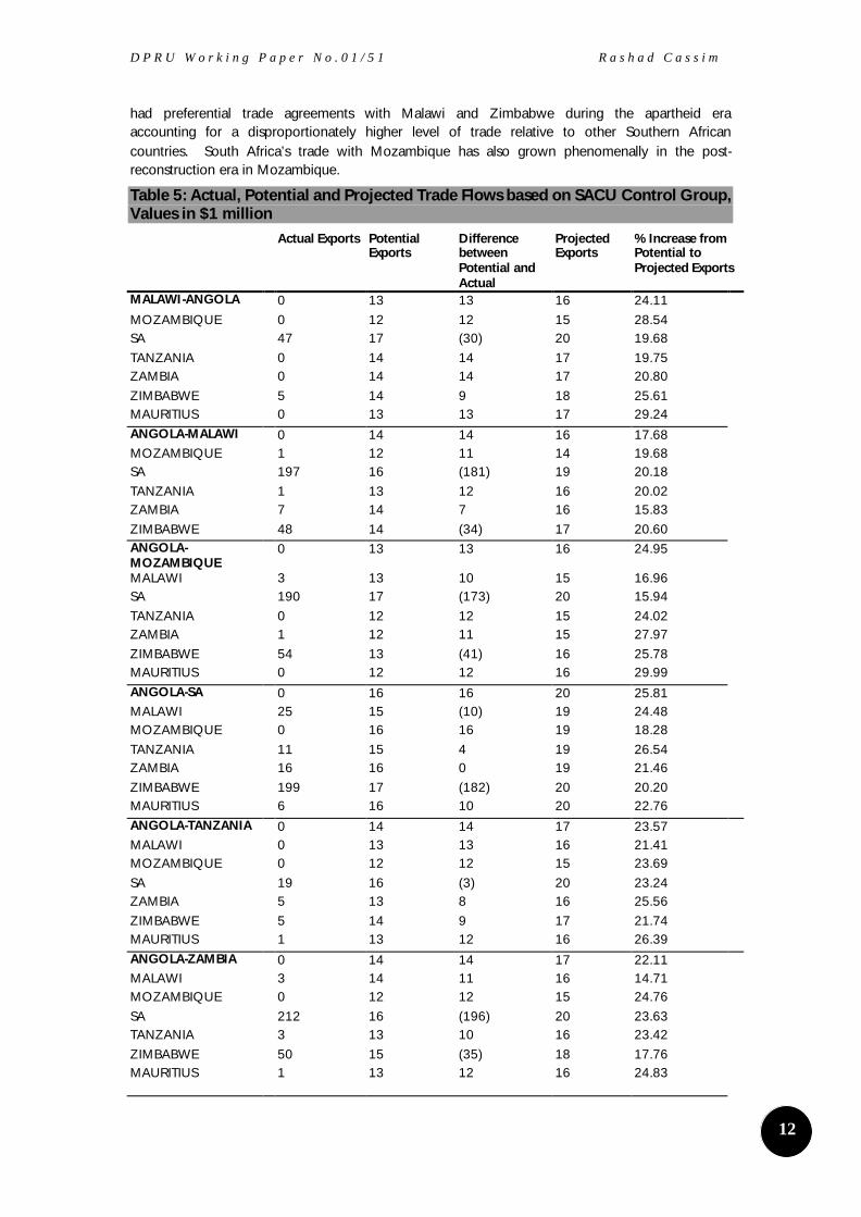
Table 5 shows actual trade flows compared to potential trade flows. Predicted trade is based on SACU as a set of reporter countries. The first column consists of actual exports based on average 1991-1994 data in millions of dollars. This is based on the trade data used in the model. The second column consists of potential or theoretical exports once the base coefficients are inserted and new values are calculated. The third column represents the difference between actual and theoretical trade.

The results are striking and in some ways very intuitive. Specific areas where potential trade is less than actual trade are mostly South African and Zimbabwean exports to the region. In the case of South Africa, in all instances, its potential exports are significantly lower than its actual exports. This is very interesting in the sense that trade patterns are currently skewed in favour of South Africa.

The negative differences between South Africa’s potential and actual trade are specifically high for Zimbabwe, Malawi and Angola. The above results also make a great deal of sense as far as South Africa’s exports to Zimbabwe, Malawi and Mozambique are concerned. South Africa has


1212

had preferential trade agreements with Malawi and Zimbabwe during the apartheid era accounting for a disproportionately higher level of trade relative to other Southern African countries. South Africa’s trade with Mozambique has also grown phenomenally in the post-reconstruction era in Mozambique.

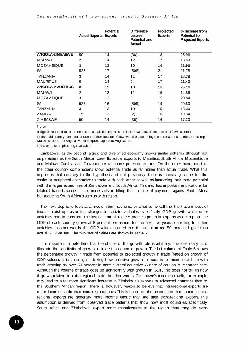
Table 5: Actual, Potential and Projected Trade Flows based on SACU Control Group, Values in $1 million

Actual Exports Potential Exports

Difference between Potential and Actual

Projected Exports

% Increase from Potential to Projected Exports

MALAWI-ANGOLA 0 13 13 16 24.11 MOZAMBIQUE 0 12 12 15 28.54 SA 47 17 (30) 20 19.68 TANZANIA 0 14 14 17 19.75 ZAMBIA 0 14 14 17 20.80 ZIMBABWE 5 14 9 18 25.61 MAURITIUS 0 13 13 17 29.24 ANGOLA-MALAWI 0 14 14 16 17.68 MOZAMBIQUE 1 12 11 14 19.68 SA 197 16 (181) 19 20.18 TANZANIA 1 13 12 16 20.02 ZAMBIA 7 14 7 16 15.83 ZIMBABWE 48 14 (34) 17 20.60 ANGOLA-MOZAMBIQUE

0 13 13 16 24.95

MALAWI 3 13 10 15 16.96 SA 190 17 (173) 20 15.94 TANZANIA 0 12 12 15 24.02 ZAMBIA 1 12 11 15 27.97 ZIMBABWE 54 13 (41) 16 25.78 MAURITIUS 0 12 12 16 29.99 ANGOLA-SA 0 16 16 20 25.81 MALAWI 25 15 (10) 19 24.48 MOZAMBIQUE 0 16 16 19 18.28 TANZANIA 11 15 4 19 26.54 ZAMBIA 16 16 0 19 21.46 ZIMBABWE 199 17 (182) 20 20.20 MAURITIUS 6 16 10 20 22.76 ANGOLA-TANZANIA 0 14 14 17 23.57 MALAWI 0 13 13 16 21.41 MOZAMBIQUE 0 12 12 15 23.69 SA 19 16 (3) 20 23.24 ZAMBIA 5 13 8 16 25.56 ZIMBABWE 5 14 9 17 21.74 MAURITIUS 1 13 12 16 26.39 ANGOLA-ZAMBIA 0 14 14 17 22.11 MALAWI 3 14 11 16 14.71 MOZAMBIQUE 0 12 12 15 24.76 SA 212 16 (196) 20 23.63 TANZANIA 3 13 10 16 23.42 ZIMBABWE 50 15 (35) 18 17.76 MAURITIUS 1 13 12 16 24.83


1313

Actual Exports

Potential Exports

Difference between Potential and Actual

Projected Exports

% Increase from Potential to Projected Exports

ANGOLA-ZIMBABWE 50 14 (36) 18 25.96 MALAWI 2 14 12 17 18.53 MOZAMBIQUE 3 13 10 16 21.96 SA 525 17 (508) 21 21.78 TANZANIA 3 14 11 17 18.38 MAURITIUS 5 14 9 17 21.43 ANGOLA-MAURITIUS 0 13 13 16 25.16 MALAWI 2 13 11 15 14.86 MOZAMBIQUE 3 12 9 15 20.84 SA 525 16 (509) 19 20.80 TANZANIA 3 13 10 15 18.30 ZAMBIA 15 13 (2) 16 19.34 ZIMBABWE 50 14 (36) 16 17.20

Notes:

i) Figures rounded of to the nearest decimal. This explains the lack of variance in the potential flows column. ii) The bold country combinations denote the direction of flow with the latter being the destination countries, for example, Malawi’s exports to Angola, Mozambique’s exports to Angola, etc. iii) Parenthesis implies negative values.

Zimbabwe, as the second largest and diversified economy shows similar patterns although not as persistent as the South African case. Its actual exports to Mauritius, South Africa, Mozambique and Malawi, Zambia and Tanzania are all above potential exports. On the other hand, most of the other country combinations show potential trade as far higher than actual trade. What this implies is that contrary to the hypothesis set out previously, there is increasing scope for the spoke or peripheral economies to trade with each other as well as increasing their trade potential with the larger economies of Zimbabwe and South Africa. This also has important implications for bilateral trade balances – not necessarily in tilting the balance of payments against South Africa but reducing South Africa’s surplus with region.

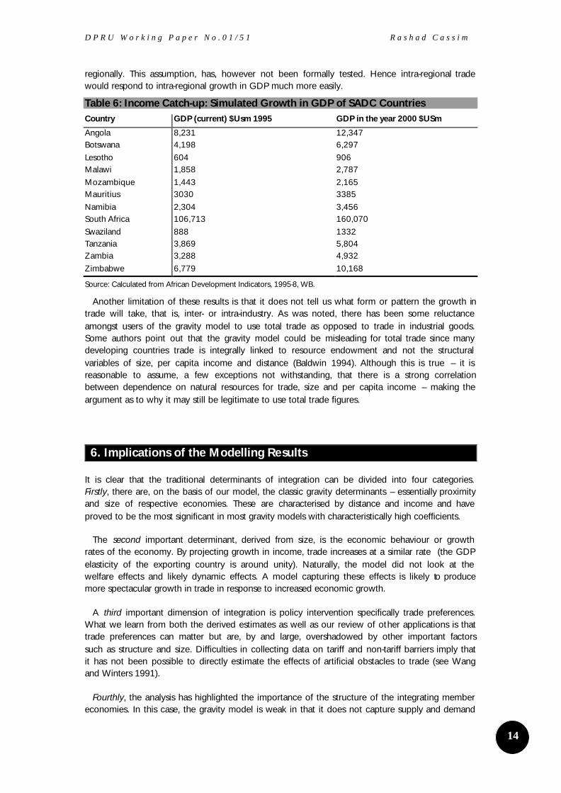
The next step is to look at a medium-term scenario, or what some call the ‘the trade impact of income catch-up’ assuming changes in certain variables, specifically GDP growth while other variables remain constant. The last column of Table 5 projects potential exports assuming that the GDP of each country grows at 8 percent per annum for the next five years controlling for other variables. In other words, the GDP values inserted into the equation are 50 percent higher than actual GDP values. The two sets of values are shown in Table 5.

It is important to note here that the choice of the growth rate is arbitrary. The idea really is to illustrate the sensitivity of growth in trade to economic growth. The last column of Table 5 shows the percentage growth in trade from potential to projected growth in trade (based on growth of GDP values). It is once again striking how sensitive growth in trade is to income catch-up with trade growing by over 50 percent in most bilateral countries. A note of caution is important here. Although the volume of trade goes up significantly with growth in GDP, this does not tell us how it grows relative to extra-regional trade. In other words, Zimbabwe’s income growth, for example, may lead to a far more significant increase in Zimbabwe’s exports to advanced countries than to the Southern African region. There is, however, reason to believe that intra-regional exports are more income-elastic than extra-regional ones This is based on the assumption that countries intra-regional exports are generally more income elastic than are their extra-regional exports. This assumption is derived from observed trade patterns that show how most countries, specifically South Africa and Zimbabwe, export more manufactures to the region than they do extra-


1414

regionally. This assumption, has, however not been formally tested. Hence intra-regional trade would respond to intra-regional growth in GDP much more easily.

Table 6: Income Catch-up: Simulated Growth in GDP of SADC Countries Country GDP (current) $Usm 1995 GDP in the year 2000 $USm

Angola 8,231 12,347 Botswana 4,198 6,297 Lesotho 604 906 Malawi 1,858 2,787 Mozambique 1,443 2,165 Mauritius 3030 3385 Namibia 2,304 3,456 South Africa 106,713 160,070 Swaziland 888 1332 Tanzania 3,869 5,804 Zambia 3,288 4,932 Zimbabwe 6,779 10,168

Source: Calculated from African Development Indicators, 1995-8, WB.

Another limitation of these results is that it does not tell us what form or pattern the growth in trade will take, that is, inter- or intra-industry. As was noted, there has been some reluctance amongst users of the gravity model to use total trade as opposed to trade in industrial goods. Some authors point out that the gravity model could be misleading for total trade since many developing countries trade is integrally linked to resource endowment and not the structural variables of size, per capita income and distance (Baldwin 1994). Although this is true – it is reasonable to assume, a few exceptions not withstanding, that there is a strong correlation between dependence on natural resources for trade, size and per capita income – making the argument as to why it may still be legitimate to use total trade figures.

6. Implications of the Modelling Results

It is clear that the traditional determinants of integration can be divided into four categories. Firstly, there are, on the basis of our model, the classic gravity determinants – essentially proximity and size of respective economies. These are characterised by distance and income and have proved to be the most significant in most gravity models with characteristically high coefficients.

The second important determinant, derived from size, is the economic behaviour or growth rates of the economy. By projecting growth in income, trade increases at a similar rate (the GDP elasticity of the exporting country is around unity). Naturally, the model did not look at the welfare effects and likely dynamic effects. A model capturing these effects is likely to produce more spectacular growth in trade in response to increased economic growth.

A third important dimension of integration is policy intervention specifically trade preferences. What we learn from both the derived estimates as well as our review of other applications is that trade preferences can matter but are, by and large, overshadowed by other important factors such as structure and size. Difficulties in collecting data on tariff and non-tariff barriers imply that it has not been possible to directly estimate the effects of artificial obstacles to trade (see Wang and Winters 1991).

Fourthly, the analysis has highlighted the importance of the structure of the integrating member economies. In this case, the gravity model is weak in that it does not capture supply and demand


1515

conditions at the micro level or the nature and behaviour of firms in a country. Because the data is aggregate data, it is also difficult to capture the level of diversification of the trade profiles of individual countries. However, in spite of the fact that the gravity model is not elaborate or detailed enough to provide more substantive clues on these issues, one broad indicative proxy for structure is the per capita income variable characterising the level of development of a specific economy. One of the ways in which the gravity approach can be tailored to look at the potential for diversification of trade potential and trade patterns is to create disaggregated samples of manufacturing trade rather than using total trade. Clearly, data constraints precluded this option here but with increasing improvement of data it will be possible to do this in the future.

Another important dimension to model is the generation of coefficients to introduce a predictive element to the overall results.13 It was noted previously that the gravity model allows one to develop a norm around which one can assess whether trade levels are unusually high or low. The question here is whether intra-regional trade has increased more rapidly than would be predicted in a systematic framework measuring normal trade? The answer is yes, according to the results here, specifically for non-SACU SADC trade.

While proximity and size are important, regional integration cannot be entirely explained by these variables. In other words, to determine the impact of distortions such as prices, product-by-product trade creation and trade diversion variables would be more useful in some ways. As the gravity model cannot distinguish between trade creation and trade diversion, one certainly cannot generalise from the increases in intra-regional trade to increases in welfare (Wang and Winters 1991:14). The model does not tell us much about welfare, or more specifically, the welfare implications of trade. More far reaching conclusions about welfare will require a multi-country regional general equilibrium model. Prices have been excluded from the gravity model for very good reasons (see Cassim 2000). However, the lack of relative prices means that we have little leverage to assess the impact of trade policy and other distortions in a behavioural sense.

Like the international literature this paper finds that all the non-dummy variables are statistically different from zero. When comparing the results of the model here to those generated by similar models, it is clear that results differ across different models. This can be attributed to the sample size, differences in sample choice and pooling. Pooling is useful but, in this case, averages are more meaningful in the sense that the sample is not likely to be influenced by wide fluctuations in the trade characteristic of many developing countries.

One of the concerns with the theoretical or projected trade flows is whether there is any way of assessing whether the model is over-estimating or under-estimating trade flows. Most of the empirical applications rarely question the efficacy of the theoretical trade flows they generate from their models.

Markheim (1994:108) argues that ex ante studies of trade policy changes uniformly underestimate the impact on trade flows. One reason why they undervalue what occurs is that changes in tariff rates invoke countries to shift larger amounts of resources towards the production and supply of exports. The gravity model on the other hand could either over-estimate or under-estimate the effects of integration. This depends on the comparator region selected. The risk of choosing the wrong comparator region was minimised by using two samples. Both produced similar results.

13 This approach is common in the literature. See Wang and Winters 1991; Baldwin 1994 and Ogunkula 1994.


1616

7. Conclusion

This paper began with a review of some calculations of potential trade in Southern Africa. Juxtaposed with these were some original calculations of trade potential. The results of different methodological approaches in measuring the impact of trade differ in some ways. There is a range of widely used techniques in measuring the impact of economic integration. These include basic descriptive analysis, to various kinds of econometric work and multi-country partial and general equilibrium analysis.

What the gravity model suggests is that a programme of intra-regional trade liberalisation could engender further trade potential in some country combinations. Indeed this will depend not only on tariff liberalisation but also on overall reduction in trade costs. In the gravity model trade in overall terms decreases from US$2314 million to US$775 million. This represents a reduction in trade of over 50 percent but increases significantly for non-SACU SADC countries’ exports to South Africa. This finding is consistent with the many other models that show actual trade in Sub-Saharan Africa is greater than potential trade (Fouratan and Prichett 1993).

A key message from the gravity exercise is that what is important is not only overall trade potential in SADC but the trade potential amongst bilateral country combinations that make up SADC. The projections of the model show that the trade potential for non-SACU SADC countries is higher than it is for SACU countries in the SADC region. This can be explained by the fact that SACU has more or less realised its trade potential in the region while the non-SACU countries have yet to realise this potential.

The Evans model, on the other hand, shows an overall increase in trade to about 12 percent if one uses short-run elasticities and to about 25 percent if one uses long-run elasticities. If the model were to be upgraded to a general equilibrium one, the trade effects are likely to be the same – except that the model is likely to give more information on factor prices and other second round effects. However, what is likely to change the results of the model more dramatically is the incorporation of scale economies and imperfect competition since additional gains can be derived from the benefits associated with a FTA when scale economies and pro-competitive effects are present.

Projected trade potential in the SADC region based on a simple, descriptive method by looking at potential trade (defined as the value of imports currently coming from the rest of the world for which at least one SSA country is making significant exports to the rest of the world) was also reviewed. The projections are nevertheless instructive and show impressive trade potential. For example, SACU’s imports from SADC in 1995 were $402 million while potential imports are estimated at $4919 million. This figure may be unrealistic but it does suggest large potential increases.

The gravity model is driven by a very different framework from other approaches. It is not so much concerned with the impact of trade liberalisation on the allocation of resources as with the extent to which reduction in transaction costs influences trade potential, controlling for other structural factors. So the impact of regional tariff liberalisation is estimated through its cost reducing impact.

It is clear that the main determinants of growth in intra-regional trade will be growth in GDP and GDP per capita amongst SADC countries and a reduction in the transaction costs to trading. However, the model shows that despite the enduring importance of these structural determinants, there are some additional factors that can also make a difference to trade. These include factors such as language differences and adjacency.


1717

An important consequence for policy is the issue of whether there is a good reason for a regional trade liberalisation strategy in lieu of, or in conjunction, with a unilateral liberalisation strategy. The results do not provide a straightforward answer. It is clear that growing integration is likely to be the result of increasing economic growth irrespective of whether this comes from unilateral or regional trade liberalisation. However, it seems that there is some scope for increased growth in intra-regional trade, without increasing growth in GDP. In most cases, predicted trade is higher than actual trade. In other words, unnecessarily high transaction costs in the Southern African region act as a bias against trade in the region and instead encourages firms to trade extra-regionally.

In summary, the results of the gravity model are very telling. They show that in the face of low economic growth, we are unlikely to see a major growth in intra-regional trade. Notwithstanding this, policy-makers should pay attention to reducing the transaction costs of trade, which in itself can play a role in integration. In other words, if countries in the region are experiencing low growth- it does not mean that policy-makers should do nothing about regional integration. There is much that can be done, but should be done in the context of broader growth strategies of which regional trade liberalisation is one small component compared to, for example, unilateral liberalisation, public sector restructuring and a range of other policies that could more directly affect growth.

To generate results that would enable us to address more specific issues, what is needed are more sophisticated proxies for transport and transaction costs, more disaggregated data preferably by sector, and further analysis of the impact of trade on resource allocation and production.

In the final analysis - the aim of this paper has not been to provide policy options or prescriptions to policy-makers. Instead, the major objective has been to provide a framework to understand the basic parameters under which intra-regional trade operates. The study demonstrated that a simple desire to see increasing intra-regional trade in the Southern Africa is the beginning and not the end of any analysis. The real work involves an assessment of the limitations that are placed on potential regional trade by the structural characteristics of the economies of trading partners as well as the policy milieu within each partner country.


1818

Appendix 1

Data and Specification Issues

Econometric Approach

The approach used here is a Tobit maximum likelihood estimation method rather than an ordinary least squared (OLS) approach and a double-log specification, instead of semi-logs to directly derive elasticities. Apart from the specific econometric approach used here, the results of the model are likely to be sensitive to the sample selection or country coverage.

Explanatory Variables

1. Distance

The distance variable has generated much discussion, partly because it is meant to capture, not only transportation costs but also the overall transaction costs of trade. There are various ways in which distance could be captured. The most obvious approach is to use road, rail, and sea or air distances in the model. An important question is what measure of distance most accurately reflects the real transaction costs of trading?

The underlying rationale is that such costs should rise with distance. Bayoumi and Eichengreen (1995), make the distinction between economic and geographic distance. The problem is that distance as a geographical concept may not be an accurate reflection of transaction costs in certain instances. For example, the transaction costs of goods from South Africa to Europe may be lower than that between Tanzania and South Africa even though distance in the latter case may be a third of the distance between the EU and South Africa.

The complexity of what to use as a proxy for transactions costs is compounded by the all-encompassing nature of these costs. Transaction costs refer to costs in obtaining information, the cost of bureaucratic processes involving government regulations and the costs of financing the transactions depending on how efficient and developed financial institutions are in specific countries. In developing countries there is the added risk of payment defaults.

Wang and Winters (1991:12) use direct rail or road distance in their gravity model for African countries. They point out that for Africa, road communication is quite poor, so that although road distance between economic centres of respective countries is much shorter than the nautical distance, the cost of overland transportation is probably higher that the cost of sea transportation. According to Jebuni (1997:367) transportation costs in Africa are high in both relative and absolute terms. Lack of shipping services forces firms to use road and in some cases rail as the mode for transporting goods. This makes the absolute costs of trading high. One implication of this is that only high-value added goods are traded. In addition, the cost of trading intra-regionally might be higher than that of trading extra-regionally.

A more nuanced approach to finding the best proxy for transportation costs in Africa emanates from the work of Ogunkola (1994: 29-30). He argues that the cost of transportation differs not only from trader to trader and time to time; it also varies with the composition of merchandise, weights and volume. In view of this problem, he introduces parcel express services, as an indicator of transportation costs. However, he shows that there is a high correlation between transportation costs and distance. In other words, transportation costs and distance are substitutable. He invariably comes to the conclusion that gravity models that employ distance as a proximate variable for transportation costs may not be all that biased.


1919

The question really is, what is the best proxy for transportation costs in Southern Africa likely to be? In Southern Africa it makes sense to use rail or road as a proxy for distance since most trade flows go through these channels. Despite the robustness of the distance variable in most of the models reviewed in the previous chapter, transportation costs represents only a component of total transaction costs.

Trade flows amongst African countries require specific attention as both the transport costs and the transaction costs are particularly high. This has to be borne in mind in the model developed later on.

Yet despite concerns about its accuracy as a proxy for trade-transactions costs, this variable, almost irrespective of how distance is measured, tends to perform well as a predictor of bilateral trade. This study will use straight-line distance between the capitals of the two countries as a proxy. This is calculated from a standard map of the world constructed to scale. The appropriateness of this proxy in the case of the Southern African region may be questioned, but for lack of data on factors, which would more closely capture the trade-transactions costs between these countries, no alternatives will be included in the study. One of the ways of making more sense of the distant variable is to complement the econometric results with more qualitative information.

2. Income

The regular source for GDP data is the World Development Report, which is also used here (World Bank, 1992-6). It is also important to note that measures of income in Southern Africa, specifically in countries such as Mozambique, understate the promotion of economic activity and trade owing to the large percentage of informal activities.

One of the difficulties of measuring economic size across countries is that exchange rates appear to deviate from the values implied by the relative prices of goods, and it is unclear whether output should be measured in terms of the official exchange rates or their purchasing power parity counterparts (UNCTAD 1998).

Market rates fail to properly reflect the purchasing power of domestic goods among economies. Purchasing power parity rates provide a better measure of relative standards. Hence the GDP values used here are based on purchasing power criteria. This is specifically important for developing countries that typically suffer from wide fluctuations in the official dollar exchange rate.

3. Dummy Variables

Dummy variables are used, amongst other things, to capture ex-post the effectiveness of trade agreements. For example, if one finds a positive coefficient of a dummy variable indicating two countries are in a preferential agreement, this implies that the agreement is trade creating. Similarly, a negative coefficient implies trade diversion (Bayoumi and Eichengreen 1995: 2).

One of the concerns that Bayoumi and Eichengreen raise is that the coefficients on dummy variables for sub-groups of countries will pick up all respects in which those countries differ in their trade performance that are not controlled for by the gravity equation. They argue (1993:3) that if all countries in a region share a common language this will tend to spuriously attribute the effects of shared language in encouraging economic links to commercial policy measures. In other words dummy variables for preferential arrangements serve as a catch basin for omitted factors. This is partly solved by the fact that major variables remain more significant than dummies. Moreover, the inclusion of dummies for language and common border will reduce the size of the catch basin.


2020

A dummy will be used to indicate the existence of bilateral trade agreements, 1 to indicate the existence of a bilateral trade agreement between counties i and j, and 0 if not. Another dummy will take account of membership of a regional integration scheme, 1 if the two countries belong to a common scheme and 0 if they do not. Cultural affinity will be proxied by a shared language and adjacency will be reflected in a dummy for a shared border.

Trade Data and the Dependent Variable

The model looks at the average of SADC trends from 1991 to 1994. Some discussion has centred on whether to use import or export data to measure bilateral trade. Elbadawi (1995:14) argues that, in principle bilateral trade flows (whether imports or exports) should be influenced by the same factors. Foroutan and Pritchett (1993) do not agree, arguing that import patterns are likely to be determined differently from export patterns especially when considering gross as opposed to net flows. They argue further that in the case of SSA using both imports and exports will assist in remedying the problem of unrecorded trade. Unrecorded trade in SSA, and also in the SADC region is a particular challenge in the estimation of trade potential as compared with actual trade. Unfortunately, it is extremely difficult to incorporate informal trade into the model. The data used in the model here is mirror import data.


2121

Appendix 2

Ex Ante Results: Model using SACU as a set of reporter countries and their trade with partners

Variable Co-efficient T-Ratio Constant -16.121 -18.886

Log (GDPI) 1.1853 22.012

Log (GDPj 0.92866 19.399

Log (Distance) -0.6270 7.612

Log (PopI) -0.20355 2.466

Log (Popj) 0.129 0.022

Adj 0.505 2.748

Lan 1.1388 7.003

Comesa 1.5887 5.053

Island 0.15887 5.052

Log ( Area I) -0.18012 -4.798

Log (Areaj) -0.21124 -6.277

No of Observations; 702 Log –likelihood test - -1711.835

Log –Likelihood ratio - - 905.4752


2222

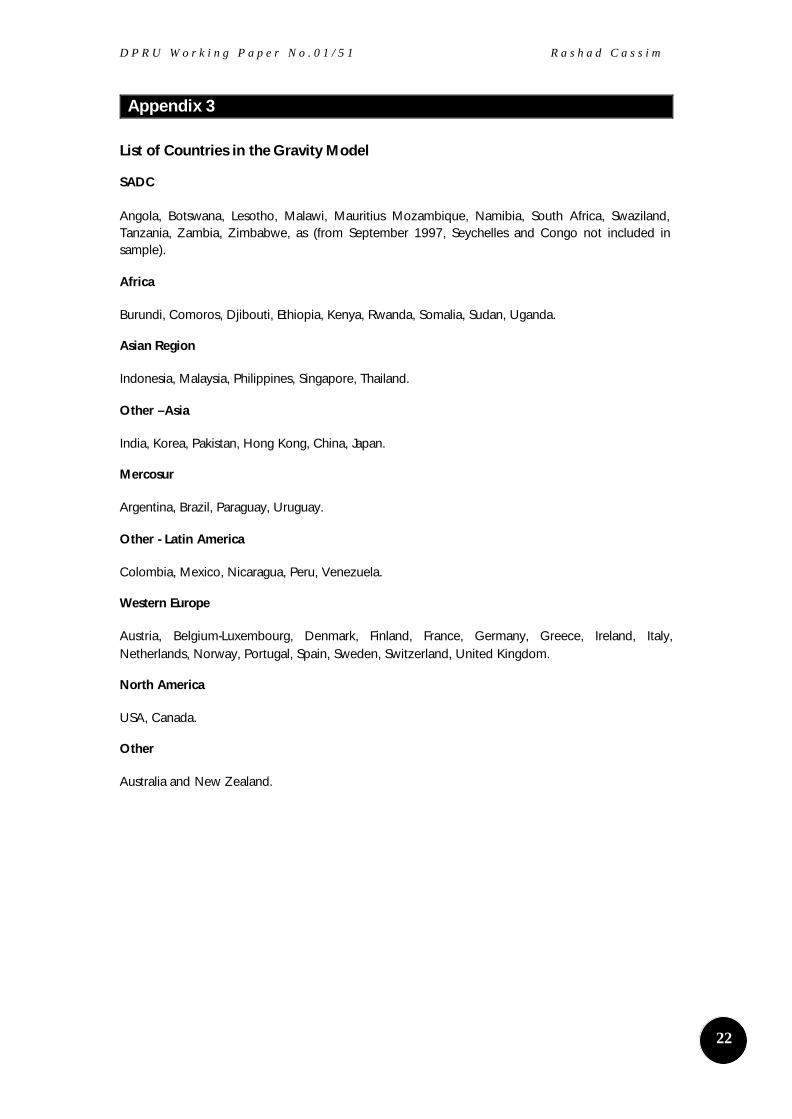
Appendix 3

List of Countries in the Gravity Model

SADC

Angola, Botswana, Lesotho, Malawi, Mauritius Mozambique, Namibia, South Africa, Swaziland, Tanzania, Zambia, Zimbabwe, as (from September 1997, Seychelles and Congo not included in sample).

Africa

Burundi, Comoros, Djibouti, Ethiopia, Kenya, Rwanda, Somalia, Sudan, Uganda.

Asian Region

Indonesia, Malaysia, Philippines, Singapore, Thailand.

Other –Asia

India, Korea, Pakistan, Hong Kong, China, Japan.

Mercosur

Argentina, Brazil, Paraguay, Uruguay.

Other - Latin America

Colombia, Mexico, Nicaragua, Peru, Venezuela.

Western Europe

Austria, Belgium-Luxembourg, Denmark, Finland, France, Germany, Greece, Ireland, Italy, Netherlands, Norway, Portugal, Spain, Sweden, Switzerland, United Kingdom.

North America

USA, Canada.

Other

Australia and New Zealand.


2323

Reference

ADB (African Development Bank) (1993) Economic Integration in Southern Africa, Volume 2, ADB, Abidjan.

Baldwin, R. (1994) Towards an integrated Europe , Centre for Economic Policy Research, London.

Bergstrand, J. (1985) The Gravity Equations in International Trade: Some Microeconomic Foundations and Empirical Evidence, Review of Economic and Statistics , 67: 474-481.

Bergstrand , J. (1989) The Generalized Gravity Equation, Monopolistic Competition, and the Factor Proportions Theory in International Trade, Review of Economic and Statistics , 71:

Cassim, R. and Hartzenburg, T. (1988) Trade Related Aspects of Southern African Regional Integration, AERC, Kenya, Nairobi, Unpublished.

Cassim, R. (2000) The Determinants of Intra-Regional Trade in Southern Africa, Unpublished Phd, University of Cape Town.

Cattaneo, N. S. (1998) The theoretical and Empirical Analysis of Trade Integration among Unequal Partners: Implications for the Southern African Development Community, Unpublished Msc Dissertation, Rhodes University, Grahamstown

Eichengreen, B. and Irwin, D. (1993), Trade Blocs, Currency Blocs and the Disintegration of World Trade in the 1930s, Centre for Economic Policy Research.

Eichengreen, B.1 and Bayoumi, T. (1995) Is Regionalism Simply A Diversion? Evidence From the Evolution of the EC and EFTA, Centre for Economic Policy Research.

Elbadawi I, (1995), The Impact of Regional Trade/Monetary schemes on Intra-Sub-Saharan African Trade, Unpublished Mimeo, AERC, Kenya.

Evans, D. (1991) Institutions and Trade Policy Reform: Sequencing and the Reform of Quantitative Controls, UNCTAD March.

Evans, D. (1996) Trade Policy Strategies for Southern Africa: Building SADC Trade Policy Capability, Report prepared for the SADC Industry and Trade Coordination Division SITCD, Institute of Development Studies, University of Sussex.

Evans, D. (1997a) Technical appendix, From Study of the Impact of the Removal of Tariffs for the Free Trade Area of the Southern African Development Community SADC, Report prepared for the SADC Industry and Trade Coordination Division SITCD, Institute of Development Studies, University of Sussex, forthcoming.

Evans, D. (1997b) The Uruguay Round and the Free Trade Area of the Southern African Development Community SADC, Draft. Mimeo, Institute of Development Studies, University of Sussex, June.

Evans, D. (1998) Options for Regional Integration in Southern Africa, Paper presented at the Trade and Industrial Policy Secretariat Forum, September, Johannesburg.

Holden, M. (1996) Economic Integration and Trade Liberalisation in Southern Africa: is there a role for South Africa? World Bank Discussion Paper No 342, World Bank, Washington DC.


2424

Koester, U. and Thomas, M. (1994) Agricultural Trade between Malawi, Tanzania, Zambia and Zimbabwe: Potential Constraints and Policy Implications in Achi Atsain et al, op.cit

Koschel, H. and Schmidt, F. N. T. (1998) Modelling of Foreign Trade in Applied General Equilibrium Models: Theoretical Approaches and sensitivity Analysis with the GEM-E3 Model, Centre for European Economic Research, Discussion paper No. 98-08.

Markheim, D. (1994) A note on predicting the trade effects of economic integration and other preferential trade agreements: an assessment, Journal of Common Market Studies, Vol. 32, No. 1.

Ogunkola, E. O. (1994) An empirical evaluation of trade potential in the economic community of West African States, AERC, Nairobi, Kenya.

von Kirchbach, F. and Roelofsen, H. (1998) African development in a Comparative Perspective, Trade in Southern African Development Community: What is the Potential for Increasing Exports to the Republic of South Africa? United Nations Conference on Trade and Development, Study No. 11, United Nations, Geneva.

Shoven, J. and Whalley, J. (1984) Applied General Equilibrium Models of Taxation and International Trade: An Introduction and Survey, Journal of Economic Literature , xxii, 1007-1051

Stewart, F. (1991) A Note on `Strategic Trade' Theory and the South in Journal of International Development, Vol 3, No 5.

Thomsen, S. (1994) Regional Integration and Multinational Production, in Cable and Henderson, opcit.

United Nations (1998) Financial Instability Growth in Africa, Trade and Development Report, United Nations Conference on Trade and Development.

Valentine, N. (1998) The SADC’s Revealed Comparative Advantage in Regional and International Trade, A background Paper to the project on an Industrial Strategy for Southern Africa, Prepared for the Industrial Strategy Project, the Development Policy Research Unit.

Vamvakidis, A. (1998) Regional Integration and Economic Growth, in The World Bank Economic Review, Vol 12 No 2.

Vaistos, C. (1978) Crisis in Regional Economic Cooperation (Integration) among Developing Countries: A Survey in World Development, Vol 6.

Waelbroeck, J. (1976) Measuring the Degree of Progress of Economic Integration in (Machlup) F(editor), Economic Integration, Worldwide, Regional and Sectoral, Macmillan Press, London.

Wang Z.K and Winters A, (1991), The Trade Potential of Eastern Europe, Centre for Economic Policy Research, Discussion paper no 610, London.

Weeks, J. and Subasat, T. (1995) Agricultural Trade Integration for Eastern and Southern Africa, ODA, March.

World Bank (1993) World Development Report 1993-7, London and New York, Oxford University Press.

rashad cassim - uct faculty of humanities · the measurement of trade creation and diversion is...

Documents