rates of convex approximation in non-hilbert spacesmdonahue/pubs/dgds.pdf · rates of convex...
TRANSCRIPT

Constr. Approx.CONSTRUCTIVE
APPROXIMATIONc© 1994 Springer-Verlag NewYork Inc.
Rates of Convex Approximation in Non-HilbertSpaces
Michael J. Donahue, Leonid Gurvits, Christian Darken, and Eduardo Sontag
Abstract.
This paper deals with sparse approximations by means of convex com-binations of elements from a predetermined “basis” subset S of a functionspace. Specifically, the focus is on the rate at which the lowest achievable
error can be reduced as larger subsets of S are allowed when constructingan approximant. The new results extend those given for Hilbert spaces byJones and Barron, including in particular a computationally attractive in-
cremental approximation scheme. Bounds are derived for broad classes ofBanach spaces; in particular, for Lp spaces with 1 < p < ∞, the O(n−1/2)bounds of Barron and Jones are recovered when p = 2.
One motivation for the questions studied here arises from the area of
“artificial neural networks,” where the problem can be stated in terms ofthe growth in the number of “neurons” (the elements of S) needed in orderto achieve a desired error rate. The focus on non-Hilbert spaces is due to
the desire to understand approximation in the more “robust” (resistant toexemplar noise) Lp, 1 ≤ p < 2 norms.
The techniques used borrow from results regarding moduli of smoothnessin functional analysis as well as from the theory of stochastic processes onfunction spaces.
1. Introduction
The subject of this paper concerns the problem of approximating elements of aBanach space X—typically presented as a space of functions—by means of finitelinear combinations of elements from a predetermined subset S of X. In contrastto classical linear approximation techniques, where optimal approximation isdesired and no penalty is imposed on the number of elements used, we areinterested here in sparse approximants, that is to say, combinations that employfew elements. In particular, we are interested in understanding the rate at whichthe achievable error can be reduced as one increases the number allowed. Suchquestions are of obvious interest in areas such as signal representation, numericalanalysis, and neural networks (see below).
AMS classification: 41A25, 46B09, 68T05
Key words and phrases: Banach space, convex combination, neural network, modulus ofsmoothness
1

2 Donahue, Gurvits, Darken, and Sontag
Rather than arbitrary linear combinations∑
i aigi, with ai’s real and gi’s inS, it turns out to be easier to understand approximations in terms of combina-tions that are subject to a prescribed upper bound on the total coefficient sum∑
i |ai|. After normalizing S and replacing it by S ∪ −S, one is led to studyingapproximations in terms of convex combinations. This is the focus of the currentwork.
To explain the known results and our new contributions, we first introducesome notation.
1.1. Optimal Approximants
Let X be a Banach space, with norm ‖ · ‖. Take any subset S ⊆ X. For eachpositive integer n, we let linnS consist of all sums
∑ni=1 aigi, with g1, . . . , gn in
S and with arbitrary real numbers a1, . . . , an, while we let conS be the set ofsuch sums with the constraint that all ai ∈ [0, 1] and
∑
i ai = 1. The distancesfrom an element f ∈ X to these spaces are denoted respectively by
‖linnS − f‖ := inf ‖h− f‖ , h ∈ linnS
and
‖conS − f‖ := inf ‖h− f‖ , h ∈ conS .
Of course, always ‖linnS − f‖ ≤ ‖conS − f‖. For each subset S ⊆ X, linS =∪nlinnS and coS = ∪nconS denote respectively the linear span and the convexhull of S. We use bars to denote closure in X; thus, for instance, coS is the closedconvex hull of S. Note that saying that f ∈ linS or f ∈ coS is the same as sayingthat limn→+∞ ‖linnS − f‖ = 0 and limn→+∞ ‖conS − f‖ = 0 respectively; inthis case, we say for short that f is (linearly or convexly) approximable by S.These distances as a function of n represent the convergence rates of the bestapproximants to the target function f . The study of such rates is standard inapproximation theory (e.g., (Powell 1981)), but the questions addressed here arenot among those classically considered.
Let φ be a positive function on the integers. We say that the space X admitsa (convex) approximation rate φ(n) if for each bounded subset S of X and eachf ∈ coS, ‖conS − f‖ = O(φ(n)). (The constant in this estimate is allowed to,and in general will, depend on S, typically through an upper bound on thenorm of elements of S.) One could of course also define the analogous linearapproximation rates; we do not do so because at this time we have no nontrivialresults to report in that regard. (The implications of the restriction to convexapproximates is examined in Appendix A.)
Jones (1992) and Barron (1991) showed that every Hilbert space admits anapproximation rate φ(n) = 1/
√n. One of our objectives is the study of such
rates for non-Hilbert spaces. To date the larger issue of convergence rates inmore general Banach spaces and in the important subclass of Lp, p 6= 2, spaceshas not been addressed. Barron (1992) showed that the same rate is obtained inthe uniform norm, but only for approximation with respect to a particular classof sets S.

Rates of Convex Approximation 3
1.2. Incremental Approximants
Jones (1992) considered the procedure of constructing approximants to f in-crementally, by forming a convex combination of the last approximant with asingle new element of S; in this case, the convergence rate in L2 is interest-ingly again O(1/
√n). Incremental approximants are especially attractive from
a computational point of view. In the neural network context, they correspondto adding one “neuron” at a time to decrease the residual error. We next definethese concepts precisely.
Again let X be a Banach space with norm ‖ · ‖. Let S ⊆ X. An incrementalsequence (for approximation in coS) is any sequence f1, f2, . . . of elements ofX so that f1 ∈ S and for each n ≥ 1 there is some gn ∈ S so that fn+1 ∈co (fn, gn).
We say that an incremental sequence f1, f2, . . . is greedy (with respect tof ∈ coS) if
‖fn+1 − f‖ = inf
‖h− f‖ | h ∈ co (fn, g) , g ∈ S
, n = 1, 2, . . . .
The set S is generally not compact, so we cannot expect the infimum to beattained. Given a positive sequence ǫ = (ǫ1, ǫ2, . . .) of allowed “slack” terms, wesay that an incremental sequence f1, f2, . . . is ε-greedy (with respect to f) if
‖fn+1 − f‖ < inf
‖h− f‖ | h ∈ co (fn, g) , g ∈ S
+ εn , n = 1, 2, . . . .
Let φ be a positive function on the integers. We say that S has an incremental(convex) scheme with rate φ(n) if there is an incremental schedule ε such that,for each f in coS and each ε-greedy incremental sequence f1, f2, . . ., it holds that
‖fn − f‖ = O(φ(n))
as n → +∞. Finally, we say that the space X admits incremental (convex)schemes with rate φ(n) if every bounded subset S of X has an incrementalscheme with rate φ(n).
The intuitive idea behind this definition is that at each stage we attemptto obtain the best approximant in the restricted subclass consisting of convexcombinations (1−λn)fn+λng, with λn in [0, 1], g in S, and fn being the previousapproximant. It is also possible to select the sequence λ1, λ2, . . . beforehand. Wesay that an incremental sequence f1, f2, . . . is ǫ-greedy (with respect to f) withconvexity schedule λ1, λ2, . . . if
‖fn+1 − f‖ < inf
‖ ((1 − λn)fn + λng) − f‖ | g ∈ S
+ εn , n = 1, 2, . . . .
One could also define the analogous linear incremental schemes, for which onedoes not require λn ∈ [0, 1], but, as before, we only report results for the convexcase.
Informally, from now on we refer to the rates for convex approximation as“optimal rates” and use the terminology “incremental rates” for the best possiblerates for incremental schemes. For any incremental sequence, fn ∈ con(S), so

4 Donahue, Gurvits, Darken, and Sontag
clearly optimal rates are always majorized by the corresponding incrementalrates.
The main objective of this paper1 is to analyze both optimal and incrementalrates in broad classes of Banach spaces, specifically including Lp, 1 ≤ p ≤ ∞.A summary of our rate bounds for the special case of the spaces Lp is givenas Table 1. In general, we find that the worst-case rate of approximation in the“robust” Lp, 1 ≤ p < 2, norms is worse than that in L2, unless some additionalconditions are imposed on the set S.
Table 1. The order of the worst-case rate of approximation in Lp. “no” means that theapproximants do not converge in the worst case.
p 1 (1, 2) [2,∞) ∞optimal 1 n−1+1/p n−1/2 1
incremental no n−1+1/p n−1/2no
1.3. Neural Nets
The problem is of general interest, but we were originally motivated by applica-tions to “artificial neural networks.” In that context the set S is typically of theform
S = g : IRd → IR | ∃ a ∈ IRd, b ∈ IR, s.t. g(x) = ±σ(a · x+ b),
where σ : IR → IR is a fixed function, called the activation or response func-tion. Typically, σ is a smooth “sigmoidal” function such as the logistic function(1 + e−x)−1, but it can be discontinuous, such as the Heaviside function (thecharacteristic function of [0,∞)). The elements of linnS are called single hiddenlayer neural networks (with activation σ and a linear output layer) with n hid-den units. For neural networks, then, the question that we investigate translatesinto the study of how the approximation error scales with the number of hiddenunits in the network.
Neural net approximation is a technique widely used in empirical studies.Mathematically, this is justified by the fact that, for each compact subset M ofIRd, restricting elements of S to M , one has that linS = C0(M), that is, linS isdense in the set of continuous functions under uniform convergence (and hencealso in most other function spaces). This density result holds under extremelyweak conditions on σ; being locally Riemann integrable and non-polynomial isenough. See for instance (Leshno et al., 1992).
Spaces Lp with p equal to or slightly greater than one are particularly impor-tant because of their usefulness for robust estimation (e.g., (Rey 1983)). In the
1 A preliminary version of some of the results presented in this paper appeared as (Darken,Donahue, Gurvits and Sontag 1993).

Rates of Convex Approximation 5
particular context of regression with neural networks, Hanson (1988) presentsexperimental results showing the superiority of Lp (p≪ 2) to L2.
1.4. Connections to Learning Theory
Of course, neural networks are closely associated with learning theory. Let usimagine that we are attempting to learn a target function that lies in the convexclosure of a predetermined set of basis functions S. Our learned estimate ofthe target function will be represented as a convex combination of a subsetof S. For each n in an increasing sequence of values of n, we optimize ourchoice of basis functions and their convex weighting over a sufficiently largedata set (the size of which may depend on n). Let us assume that the problemis “learnable”, e.g., that over the class of probability measures of interest onthe domain of the functions in S, the difference between one’s estimates of theerror based on examples must converge to the true error uniformly over allpossible approximants. Then the generalization error (expected loss over thetrue exemplar distribution) must go to zero at least as fast as the order of theupper bounds in this work. Thus our bounds represent a guarantee of how fastgeneralization error will decrease in the limiting case when exemplars are socheap that we do not care how many we use during training.
Moreover, since for error functions that are Lp norms our bounds are tight, wecan say something even stronger in this case. For Lp, there exists a set of basisfunctions and a function in their convex hull such that no matter how manyexamples are used in training, the error can decrease no faster than the boundswe have provided. Thus, our results exhibit a worst-case speed limitation forlearning.
1.5. Contents of the Paper
It is a triviality that optimal approximants to approximable functions alwaysconverge. However, the rates of convergence depend critically upon the structureof the space. In some spaces, like L1, there exist target functions for which therate can be made arbitrarily slow (Sect. 2.1). In Banach spaces of (Rademacher)type t with t > 1, however, a rate bound of O(n−1+1/t) is obtained (Sect. 2.2).For Lp spaces these results specialize to those of Table 1. Particular examplesof Lp spaces are given to show that the orders given in our bounds cannot ingeneral be sharpened (Sect. 2.3).
Section 3 studies incremental approximation. A particularly interesting aspectof these results is that the new element of S added to the incremental approxi-mant is not required to be the best possible choice. Instead, the new element canmeet a less stringent test (Theorem 3.5). Also, the convex combination of theelements included in the approximant is not optimized. Instead a simple averageis used. (This is an example of a fixed convexity schedule, as defined in Sect. 1.2.)Thus, our incremental approximants are the simplest yet studied, simpler eventhan those of (Jones 1992). Nonetheless, the same worst-case order is obtainedfor these approximants on Lp, 1 < p < ∞, as for the optimal approximant.

6 Donahue, Gurvits, Darken, and Sontag
In more general spaces, the incremental approximants may not even converge(Sect. 3.1). However, if the space has a modulus of smoothness of power typegreater than one, or is of Rademacher type t, then rate bounds can be given(Sects. 3.2 and 3.3).
Both optimal and incremental convergence rates may be improved if S hasspecial structure (Sect. 4). In particular, we provide some analysis of the situa-tion where S is a finite-VC dimension set of indicator functions and the sup normis to be used, which is a common setting for neural network approximation.
2. Optimal Approximants
In this section we study rates of convergence for optimal convex approximates.To illustrate the fact that the issue is nontrivial, we begin by identifying a classof spaces for which the best possible rate φ(n) is constant, that is to say, nonontrivial rate is possible (Theorem 2.3). This class includes infinite dimensionalL1 and L∞ (or C(X)) spaces.
In Theorem 2.5 we then study general bounds valid for spaces of (Rademacher)type t. It is well-known that Lp spaces with 1 ≤ p < ∞ are of type minp, 2(Ledoux and Talagrand 1991); on this basis an explicit specialization to Lp isgiven in Corollary 2.6.
We then close this section with explicit examples showing that the obtainedbounds are tight.
2.1. Examples of Spaces Where No Rate Bound is Possible
In some spaces, the worst-case rate of convergence of optimal approximants canbe shown to be arbitrarily slow.
Lemma 2.1. Let (an) be a positive, convex (an + an+2 ≥ 2an+1) sequenceconverging to 0. Define a0 = 2a1 and bn = an−1 − an. Let S = a0ek, whereek is the canonical basis in l1, and consider f = (bn) as an element of l1.Then f ∈ coS and
‖linNS − f‖ = aN for all N.(2.1)
Proof. Note that∑∞
n=1 bn/a0 = 1, so clearly f ∈ coS. By convexity (bn) is anon-increasing sequence, so
‖linNS − f‖ =∞∑
i=N+1
bi =∞∑
i=N+1
ai−1 − ai = aN .(2.2)
⊓⊔
Consider next the space l∞. Let ǫk be an enumeration of all −1, 0, 1-valuedsequences that are eventually constant, i.e., ǫk(n) ∈ −1, 0, 1 for all n ∈ IN, andfor each k there exists an N such that ǫk(n) = ǫk(N) for all n > N . For each n,let gn ∈ l∞ be the sequence gn(k) = ǫk(n), and define the map T : l1 → l∞ by

Rates of Convex Approximation 7
T (en) = gn. The reader may check that T is an isometric embedding. ThereforeT carries the example of Lemma 2.1 into l∞.
What happens in c0, the space of all sequences converging to 0? We will nowconstruct a projection from T (l1) into c0 that will retain the desired convergencerate. We will need, however, the extra restriction that the sequence (an) bestrictly convex, i.e., that an + an+2 > 2an+1.
Let bn = an−1 − an as before, and define the auxiliary sequences
cN = minn ∈ IN | bn < aNcN = minn ∈ IN | n > N + 1 and an < bN − bN+1.
The sequence c is well defined because aN > 0 for all N and bn ↓ 0. Similarly,c is well defined since an ↓ 0 and by strict convexity bN − bN+1 > 0. Note thatcN ≤ N + 1 < N + 2 ≤ cN . Moreover, cN (and hence cN ) goes to infinity withN since bn > 0 for each n while aN ↓ 0.
Next define for each N ∈ IN,
AN = k ∈ IN | ǫk(n) = 0 for n < cN and ǫk(n) = ǫk(cN + 1) for n > cN,and define for convenience the single element set A0 = k | ǫk = δk, whereδk(n) is the sequence that is 1 for n = k and 0 otherwise. Then let A = ∪NAN .
Let P be the projection that sends an element h of l∞ to the sequenceP (h)(k) = h(k) if k ∈ A and P (h)(k) = 0 otherwise. Notice that if ǫk(n) 6= 0,then k 6∈ AN for all N such that n < cN . Since cN → ∞, if follows that thereexists for each n only finitely many k’s in A such that ǫk(n) 6= 0. (Each AN is afinite set.) Therefore P (gn) = P T (en) ∈ c0 for each n, i.e., P T : l1 → c0.
It remains to show that
‖P T (f) − linNP T (S)‖ = aN .
Let us introduce the notation h for P T (h), h ∈ l1, and similarly S for P T (S).It is clear that ‖f−linN S‖ ≤ aN , since T is an isometry and ‖P‖ = 1. To examine
the bound from below, let fN =∑N
n=1 dnemnbe an arbitrary element of linN S,
where m1,m2, . . . ,mN is a sampling of IN of size N . We aim to produce ak0 ∈ A such that fN (k0) = 0 and f(k0) ≥ aN , since then
‖f − fN‖ = supk∈A
|f(k) − fN (k)| ≥ |f(k0) − fN (k0)| ≥ aN .
Let n0 = min(IN\m1,m2, . . . ,mN). If n0 < cN , select k0 such that ǫk0= δn0
.If n0 = N + 1 (which is the largest possible value for n0), select k0 such thatǫk0
(n) = 0 for n ≤ N and = 1 otherwise. It follows from cN ≤ N +1 that k0 ∈ Ain either event, and clearly fN (k0) = 0. Moreover, in the first case f(k0) = bn0
≥aN by the definition of cN , while in the second case, f(k0) =
∑∞n=N+1 bn = aN .
Lastly, consider the case cN ≤ n0 ≤ N . Select k0 so that ǫk0(n) = 0 if
n ∈ m1,m2, . . . ,mN or if n > cN , and ǫk0(n) = 1 otherwise. This sequence is
guaranteed to be in AN , and fN (k0) = 0. Moreover,
f(k0) =
cN∑
n=cN
bnǫk0(n) ≥ bN +
cN∑
n=N+2
bn.

8 Donahue, Gurvits, Darken, and Sontag
The inequality holds because ǫk0(n) = 1 for at least one n ≤ N , and (bn) is a
decreasing sequence. It then follows from the definition of cN that
bN +
cN∑
n=N+2
bn = bN + aN+1 − acN> aN ,
so ‖f − fN‖ ≥ aN , completing the proof.
Lemma 2.2. Let (an) be a positive, strictly convex (an + an+2 > 2an+1) se-quence converging to 0. Then there exists a bounded set S ⊂ c0 (with ‖g‖ ≤ 2a1
for all g ∈ S) and f ∈ coS such that
‖f − linNS‖ = aN for all N ∈ IN.
An alternate method of proof is to replace the projection P in the discussionabove with a map T ′ : l∞ → c0 defined by T ′(h)(k) = δkh(k), where δk ↓ 0 iscarefully chosen (as a function of (an)) to preserve the inequality ‖T ′ T (f) −linNT
′ T (S)‖ ≥ aN . The details are left to the reader.In either method, the constructed base set S ⊂ c0 depends on the rate sequence
(an). It is interesting to compare this with the situation in l1 and l∞, where theset S is universal, i.e., independent of (an). (Though the limit function f ∈ coSdoes vary with (an).)
The preceding discussion showing the absence of a rate bound in l∞ reliedupon an isometric embedding of l1 into l∞. The same argument can be used ifwe have only an isomorphic embedding, i.e., a bounded linear map with boundedinverse. Combining this with the two preceding lemmas gives
Theorem 2.3. Let X be a Banach space with a subspace isomorphic to eitherl1 or c0. Then for any positive sequence (an) converging to 0, it is possible toconstruct a bounded set S and f ∈ coS such that
‖coNS − f‖ ≥ ‖linNS − f‖ ≥ aN .(2.3)
Proof. If (an) is not convex, then replace it with a strictly convex sequence (an)converging to zero such that an ≥ an for all n. This is a well-known construction,for example (Stromberg 1981, p. 515). The result then follows from Lemmas 2.1and 2.2. ⊓⊔
If a Banach space contains a subspace isomorphic to l1 or c0, then it is notreflexive. The converse is not true, though there are a variety of results that doimply the existence of subspaces isomorphic to l1 or c0, and such results combinewith Theorem 2.3 to identify spaces with arbitrarily slow convergence of the typediscussed. For example:
Theorem 2.4. [(Lindenstrauss and Tzafriri 1979, p. 35)] A Banach lattice Xis reflexive if and only if no subspace of X is isomorphic to l1 or c0.
Rates of Convex Approximation 9
This theorem implies that examples of arbitrarily slow convergence exist inL1[0, 1] and C[0, 1], although in these cases it is also easy to construct the embed-dings directly (Darken et al. 1993). Related results can be found in (Bessaga andPelczynski 1958), (Rosenthal 1974), (Rosenthal 1994), and (Gowers preprint).
In Section 3 we will show that a condition somewhat stronger than reflexivity(uniform smoothness) guarantees convergence of incremental approximates. Inthe next section, however, we show that a condition unrelated to reflexivity (theRademacher type property) can guarantee convergence of optimal approximantsand even give bounds on convergence rates.
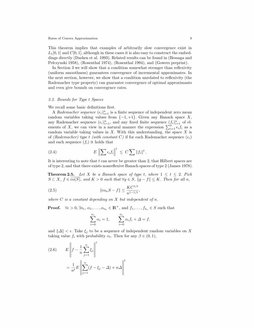
2.2. Bounds for Type t Spaces
We recall some basic definitions first.A Rademacher sequence (ǫi)
ni=1 is a finite sequence of independent zero mean
random variables taking values from −1,+1. Given any Banach space X,any Rademacher sequence (ǫi)
ni=1, and any fixed finite sequence (fi)
ni=1 of el-
ements of X, we can view in a natural manner the expression∑n
i=1 ǫifi as arandom variable taking values in X. With this understanding, the space X isof (Rademacher) type t (with constant C) if for each Rademacher sequence (ǫi)and each sequence (fi) it holds that
E∥
∥
∥
∑
ǫifi
∥
∥
∥
t
≤ C∑
‖fi‖t .(2.4)
It is interesting to note that t can never be greater than 2, that Hilbert spaces areof type 2, and that there exists nonreflexive Banach spaces of type 2 (James 1978).
Theorem 2.5. Let X be a Banach space of type t, where 1 ≤ t ≤ 2. PickS ⊂ X, f ∈ co(S), and K > 0 such that ∀g ∈ S, ‖g − f‖ ≤ K. Then for all n,
‖conS − f‖ ≤ KC1/t
n1−1/t,(2.5)
where C is a constant depending on X but independent of n.
Proof. ∀ǫ > 0,∃nǫ, α1, . . . , αnǫ∈ IR+, and f1, . . . , fnǫ
∈ S such that
nǫ∑
i=0
αi = 1,
nǫ∑
i=0
αifi +∆ = f,
and ‖∆‖ < ǫ. Take ξj to be a sequence of independent random variables on Xtaking value fi with probability αi. Then for any β ∈ (0, 1),
E
∥
∥
∥
∥
∥
∥
f − 1
n
n∑
j=1
ξj
∥
∥
∥
∥
∥
∥
t
(2.6)
=1
ntE
∥
∥
∥
∥
∥
∥
n∑
j=1
(f − ξj −∆) + n∆
∥
∥
∥
∥
∥
∥
t

10 Donahue, Gurvits, Darken, and Sontag
≤ 1
ntE
(1 − β)
∥
∥
∥
∑nj=1(f − ξj −∆)
∥
∥
∥
1 − β+ βn
‖∆‖β
t
≤ 1
nt
(1 − β)E
∥
∥
∥
∑nj=1(f − ξj −∆)
∥
∥
∥
1 − β
t
+ β
(
n ‖∆‖β
)t
=1
nt(1 − β)t−1E
∥
∥
∥
∥
∥
∥
n∑
j=1
(f − ξj −∆)
∥
∥
∥
∥
∥
∥
t
+1
βt−1‖∆‖t
,
which follows because φ(x) = xt is a convex function for 1 ≤ t ≤ 2. Since therange of ξj has finitely many values and the space is type t, by (Ledoux andTalagrand 1991, Prop. 9.11, p. 248) it follows that:
E
∥
∥
∥
∥
∥
∥
n∑
j=1
(f − ξj −∆)
∥
∥
∥
∥
∥
∥
t
≤ C
n∑
j=1
E ‖f − ξj −∆‖t.(2.7)
On the other hand, we have:
E‖f − ξ1 −∆‖t =
nǫ∑
i=1
αi‖f − fi −∆‖t(2.8)
≤nǫ∑
i=1
αi (‖f − fi‖ + ‖∆‖)t
<
nǫ∑
i=1
αi(K + ǫ)t
= (K + ǫ)t.
Without loss of generality, assume 0 < ǫ < 1 and take β = ǫ. Then combining(2.6), (2.7), and (2.8),
E
∥
∥
∥
∥
∥
∥
f − 1
n
n∑
j=1
ξj
∥
∥
∥
∥
∥
∥
t
<C(K + ǫ)t
nt−1(1 − ǫ)t−1+ ǫ.
We conclude that for some realization of the ξj (labeled gj) the inequality musthold, i.e.,
∥
∥
∥
∥
∥
∥
f − 1
n
n∑
j=1
gj
∥
∥
∥
∥
∥
∥
t
<C(K + ǫ)t
nt−1(1 − ǫ)t−1+ ǫ.
Taking the infimum with respect to all ǫ > 0 proves the theorem. ⊓⊔

Rates of Convex Approximation 11
We now give a specialization to Lp, 1 ≤ p < ∞. These spaces are of typet = minp, 2. From (Haagerup 1982) we find that the best value for C in (2.5)
is 1 if 1 ≤ p ≤ 2 and√
2 [Γ ((p+ 1)/2)/√π]
1/pif 2 < p < ∞. One may use
Stirling’s formula to get an asymptotic formula for the latter expression.
Corollary 2.6. Let X be an Lp space with 1 ≤ p < ∞. Suppose S ⊂ X,f ∈ coS, and K > 0 such that ∀g ∈ S, ‖g − f‖ ≤ K. Then for all n,
‖conS − f‖ ≤ KCp
n1−1/t,(2.9)
where t = minp, 2, and Cp = 1 if 1 ≤ p ≤ 2 and Cp =√
2 [Γ ((p+ 1)/2)/√π]
1/p
for 2 < p <∞. For large p, Cp ∼√
p/e.
2.3. Tightness of Rate Bounds
In this section we show that order of the rate bound given for Lp in (2.9) istight. That is, we give specific examples of Lp spaces and subsets S with targetfunctions f ∈ coS where optimal approximants converge with the specified order.
Theorem 2.7. There exists S ⊆ lp, 1 < p < ∞, and f ∈ coS such that‖conS − f‖p = Kn−1+1/p where K = supg∈S ‖f − g‖p.
Proof. Let S consist of the elements of the canonical basis for lp. Then f := 0is in the closed convex hull of S and supg∈S ‖f − g‖p = 1. Let fn be an elementof conS that is to approximate 0. So fn is of the form fn =
∑nk=1 akgnk
, whereeach gnk
is an element of S, and the ak are non-negative and sum to 1. Withoutloss of generality, we may assume the gnk
are distinct, since otherwise we wouldbe effectively working in comS with m < n. Then
‖fn − 0‖p =
n∑
k=1
apk.
It is easy to see that the error is minimized by taking the ak’s all equal, namely∀k, ak = 1/n (Jensen). Therefore
‖fn − 0‖ ≥ n(1−p)/p = n−1+1/p.
⊓⊔
Next we show that the O(n−1/2) bound for Lp, 2 < p < ∞, is tight (seeCorollary 2.6). We borrow from computer science the notation ψ(n) = Ω(φ(n))to mean that there is a constant C > 0 so that ψ(n)/φ(n) ≥ C for all n largeenough. For the purposes of the next result, we say a space Lp is admissible ifthere exists a Rademacher sequence definable on it; for instance, Lp(0, 1) withthe usual Lebesgue measure is one such space.
Proposition 2.8. For any admissible Lp, 2 < p < ∞, there exists a subset Sand an f ∈ coS such that ‖conS − f‖p = Ω(n−1/2).

12 Donahue, Gurvits, Darken, and Sontag
Proof. Let ξi, i.i.d. on -1,+1, be a Rademacher sequence. Define S = ξi,which is a subset of the unit ball in Lp. Using the upper bound of Khintchine’sInequality (Khintchine 1923; Ledoux and Talagrand 1991, Lemma 4.1, p. 91),one can show that 0 ∈ coS. Suppose the best approximation of 0 by a convexsum of n elements of S is
∑ni=1 αiξk(i). Then by the lower bound of Khintchine’s
Inequality,∥
∥
∥
∥
∥
n∑
i=1
αiξk(i)
∥
∥
∥
∥
∥
Lp
≥ Ap
√
∑
i
α2i = Ap‖(αi)‖l2 .
But we have already given an example in l2 (in the proof of Theorem 2.7) forwhich the last term is Ω(n−1/2). ⊓⊔
3. Incremental Approximants
We now start the study of incremental approximation schemes. Unlike the situ-ation with optimal approximation, incremental approximations are not guaran-teed to even converge. In general, the convergence of incremental schemes ap-pears to be intimately tied to the concept of norm smoothness. In Theorem 3.1we show that smoothness is equivalent to at least a monotonic decrease of theerror, and then in Theorem 3.4 it is proved that uniform smoothness is a suffi-cient condition to guarantee convergence. (It is possible to construct a smoothspace with an ǫ-greedy sequence that does not converge—Appendix D. However,if an ǫ-greedy sequence converges, then it can only converge to the desired targetfunction—Corollary 3.2.)
In Sects. 3.2 and 3.3 we study upper bounds on the rate of convergence forspaces with modulus of smoothness of power type greater than 1 and for spacesof (Rademacher) type t, 1 < t ≤ 2. The Lp spaces, 1 < p < ∞, are examplesof spaces with modulus of smoothness of power type t = min(p, 2) (see Ap-pendix B), which themselves sit inside the more general class of spaces of typet. (See, for example, (Lindenstrauss and Tzafriri 1979, p. 78; Deville et al. 1993,p. 166), while (James 1978) shows that the containment is strict. See also (Figieland Pisier 1974).) The upper bounds obtained for incremental approximationerror in the power type spaces agree with the bounds for optimal approximationerror obtained in Sect. 2.2 (albeit with a slightly larger constant of proportional-ity), which were shown to be the best possible in Sect. 2.3. Therefore, little is lostby using incremental approximates instead of optimal approximates, at least inworst-case settings. The incremental convergence bounds obtained in Sect. 3.3for type-t spaces are only slightly weaker than the optimal approximation errorbounds obtained in Sect. 2.2
3.1. Convergence of Greedy Approximants
The first remark is that for some spaces there may not exist any nondecreasingrate whatsoever. In the terminology given in the introduction, it may be the case

Rates of Convex Approximation 13
that there are greedy incremental sequences for f for which ‖fn − f‖ 6→ 0. Thiswill happen in particular if there are a set S and two elements f 6= fn ∈ coS sothat for each g ∈ S and each h ∈ co (fn, g) different from fn, ‖h−f‖ > ‖fn−f‖;in that case, the successive minimizations result in the sequence fn, fn, . . ., whichdoesn’t converge to f . Geometrically, convergence of incremental approximantscan fail to occur if the unit ball for the norm has a sharp corner. This is illustratedby the example in Fig. 1, for the plane IR2 under the L1 norm. In order to use theintuition gained from this example, we need a number of standard but perhapsless-known notions from functional analysis.
@
@@@
@@
@@
q (0, 0)
q fn
qg1 qg2
Fig. 1. Incremental approximants may fail to converge in some spaces. Consider approximatingf = (0, 0) by linear combinations of elements from fn, g1, g2 according to the L1(IR2) metric.
The best approximant by one point is fn. The rotated square is the contour of the norm aboutf on which fn lies. The best approximant by a linear combination of fn and g1 or g2 is onceagain fn. Thus even though f is in the convex hull of fn, g1, g2, incremental approximants
fail to converge or even to decrease monotonically.
If X is a Banach space and f 6= 0 is an element of X, a peak functional forf is a bounded linear operator, that is, an element F ∈ X∗, that has norm= 1 and satisfies F (f) = ‖f‖. (The existence for each f 6= 0 of at least onepeak functional is guaranteed by the Hahn-Banach Theorem.) Geometrically,one may think of the null space of F − ‖f‖ as a hyperplane tangent at f to theball centered at the origin of radius ‖f‖. (For Hilbert spaces, there is a uniquepeak functional for each f , which can be identified with (1/‖f‖)f acting byinner products.) The space X is said to be smooth if for each f there is a uniquepeak functional. (Roughly, this means that balls in X have no “corners.”) Themodulus of smoothness of any Banach space X is the function ρ : IR≥0 → IR≥0
defined by
ρ(r) :=1
2
(
sup ‖f‖=‖g‖=1 ‖f + rg‖ + ‖f − rg‖ − 2)
Note that, by sub-additivity of norms, always ρ(r) ≤ r. For Hilbert spaces,one has ρ(r) =
√1 + r2 − 1. A Banach space is said to be uniformly smooth
if ρ(r) = o(r) as r → 0; in particular, Hilbert spaces are uniformly smooth,but so are Lp spaces with 1 < p < ∞, as is reviewed in Appendix B. (Hereone has an upper bound of the type ρ(r) < crt, for some t > 1, which implies

14 Donahue, Gurvits, Darken, and Sontag
uniform smoothness.) As a remark, we point out that uniform smooth spaces arein particular smooth. Moreover, it can be shown that uniformly smooth spacesare also reflexive, though the converse implication does not hold.
The next result implies that greedy approximants always result in monotoni-cally decreasing error if and only if the space is smooth. In particular, if the spaceis not smooth, then one can not expect greedy (or even ǫ-greedy) incrementalsequences to converge. (Since one may always consider the translate S − f aswell as a translation by f of all elements in a greedy sequence, no generality islost in taking f = 0.)
Theorem 3.1. Let X be Banach space. Then:
1. Assume that X is smooth, and pick any S ⊂ X so that 0 ∈ coS. Then foreach nonzero f ∈ X there is some g ∈ S and some f ∈ co(f, g) differentfrom f so that ‖f‖ < ‖f‖.
2. Conversely, if X is not smooth, then there exist an S ⊂ X so that 0 ∈ coSand an f ∈ S so that, for every g ∈ S and every f ∈ co(f, g) differentfrom f , ‖f‖ > ‖f‖.
Proof. Assume that X is smooth, and let S and f be as in the statement. LetF be the (unique) peak functional for f . There must be some g ∈ S for which
F (g) < ‖f‖/2 ,(3.10)
since otherwise h ∈ X | F (h) = ‖f‖/2 would be a hyperplane separating co(S)from 0 ∈ coS. Define
fλ = (1 − λ)f + λg for λ ∈ [0, 1].
We wish to show that ‖fλ‖ < ‖f‖ for some λ ∈ (0, 1], as this will establish thefirst part of the Theorem. For this, consider the peak functional Fλ for fλ. Notethat
limλ↓0
Fλ(f) = limλ↓0
Fλ(fλ) + Fλ(f − fλ) = limλ↓0
‖fλ‖ = ‖f‖.(3.11)
The unit ball in X∗ is weak-∗ compact (Alaoglu), so the net (Fλ)λ∈(0,1) (whereλ ↓ 0) has a convergent subnet, say Fλα
→ F ∗, with ‖F ∗‖ ≤ 1. In particular,Fλα
(f) → F ∗(f), so it follows from (3.11) that F ∗(f) = ‖f‖, and hence F ∗
is a peak functional for f . But X is smooth, so F ∗ = F . Thus there existsλ0 ∈ (0, 1] such that |Fλ0
(g) − F (g)| < ‖f‖/2, which combines with (3.10) togive Fλ0
(g) < ‖f‖. Therefore
‖fλ0‖ = Fλ0
(fλ0) = (1 − λ0)Fλ0
(f) + λ0Fλ0(g) < ‖f‖,
since λ0 > 0. This proves the first assertion.We now prove the converse. Since X is not smooth, there is some unit vector
f with two distinct peak functionals F and F ′. Since F 6= F ′, there is someh ∈ X so that F (h) 6= F ′(h). Let
g := h−(
F (h) + F ′(h)
2
)
f .

Rates of Convex Approximation 15
Note that F (g) + F ′(g) = 0 and F ′(g) 6= 0; scaling g, we may assume thatF ′(g) = 2. Consider now the set S = f, g1, g2, where g1 = g and g2 = −g; notethat 0 ∈ coS. This provides the needed counterexample, since
‖(1 − λ)f + λg1‖ ≥ F ′ ((1 − λ)f + λg) = 1 + λ > 1 = ‖f‖
and
‖(1 − λ)f + λg2‖ ≥ F ((1 − λ)f − λg) = 1 + λ > 1 = ‖f‖
for each λ > 0. ⊓⊔
It is interesting to remark that, for the set S built in the last part of the proof,even elements in the affine span of f and g1 (or of f and g2) have norm > 1 ifdistinct from f , that is, the inequalities hold in fact for all λ 6= 0. (For λ < 0,interchange F and F ′ in the last pair of equations.)
It is an easy consequence of the first part of Theorem 3.1 that greedy incre-mental approximates in a smooth Banach space can converge only to the targetfunction:
Corollary 3.2. Let X be a smooth Banach space with S ⊂ X. Let f ∈ coSand suppose f1, f2, . . . is an incremental ǫ-greedy sequence with respect to f ,where the schedule ǫ1, ǫ2, . . . converges to 0. If the sequence (fn) converges, thenit converges to f .
Proof. Without loss of generality, we may assume that f = 0. Suppose limn fn =f∞ 6= 0. Then by the first part of Theorem 3.1, there exists g ∈ S and λ ∈ [0, 1]such that ‖(1 − λ)f∞ + λg‖ < ‖f∞‖. Define δ = ‖f∞‖ − ‖(1 − λ)f∞ + λg‖,and choose N large enough so ‖f∞ − fn‖ < δ/3 and ǫn < δ/3 for all n > N .Fix n > N . Then ‖(1 − λ)fn + λg‖ < ‖f∞‖ − 2δ/3, but (fn) is ǫ-greedy, whichimplies ‖fn+1‖ < ‖f∞‖ − δ/3. But this is impossible since by choice of N ,‖f∞ − fn+1‖ < δ/3. Therefore the limit f∞ = 0, as desired. ⊓⊔
It is possible, however, to have an ǫ-greedy sequence that fails to converge.See Appendix D. This situation is avoided if X is uniformly smooth, as we shallsee below. But first we need a technical lemma that captures the geometricproperties of smoothness necessary to obtain stepwise estimates of convergence.This lemma is used not only in Theorem 3.4, but also throughout Sect. 3.2.
Lemma 3.3. Let X be a Banach space with modulus of smoothness ρ(u), andlet S ⊂ X. Assume that 0 ∈ co(S) and let f 6= 0 be an element of co(S). Let Fbe a peak functional for f . Then
‖(1 − λ)f + λg‖ ≤ (1 − λ)
[
1 + 2ρ
(
λ‖g‖(1 − λ)‖f‖
)]
‖f‖ + λF (g),(3.12)
for all 0 ≤ λ < 1 and all g ∈ S. Furthermore, for any ǫ > 0, there exists a g ∈ Ssuch that F (g) < ǫ.

16 Donahue, Gurvits, Darken, and Sontag
Proof. Pick any 0 ≤ λ < 1 and g ∈ S. If g = 0 then (3.12) is trivially satisfied,so assume g 6= 0.
Define h = f+ug/‖g‖ and h∗ = f−ug/‖g‖ for u ≥ 0. Then from the definitionof the modulus of smoothness we have
‖h‖ + ‖h∗‖ ≤ 2‖f‖ [1 + ρ(u/‖f‖)] .
But
‖h∗‖ ≥ F
(
f − u
‖g‖g)
= ‖f‖ − uF (g)/‖g‖.
Therefore
‖h‖ ≤ ‖f‖ (1 + 2ρ(u/‖f‖)) + uF (g)/‖g‖.(3.13)
If we set u = λ‖g‖/(1 − λ), we get
(1 − λ)f + λg = (1 − λ)h,
which combines with (3.13) to prove (3.12).Finally, given ǫ > 0, suppose there is no g ∈ S such that F (g) < ǫ. Then the
affine hyperplane h ∈ X | F (h) = ǫ/2 would separate S from 0, contradicting0 ∈ co(S). ⊓⊔
Theorem 3.4. Let X be a uniformly smooth Banach space. Let S be a boundedsubset of X and let f ∈ co(S) be given, and let (ǫn) be an incremental schedulewith
∑∞k=1 ǫk <∞. Then any ǫ-greedy (with respect to f) incremental sequence
(fn) ⊂ coS converges to f .
Proof. Pick K ≥ supg∈S ‖f − g‖, and let (fn) be an ǫ-greedy incrementalsequence. Define
an := ‖fn − f‖.
We want to show that an → 0. To this end, let a∞ = lim infn→∞ an. Since (fn)
is ǫ-greedy, an+1 ≤ an + ǫn and an+m ≤ an +∑m−1
k=n ǫk. But∑∞
k=n ǫk → 0 asn→ ∞, so in fact a∞ = limn→∞ an. Suppose a∞ > 0. Then from the definitionof ǫ-greedy and (3.12), it follows that
an+1 ≤ infλ,g
(1 − λ)
[
1 + 2ρ
(
λK
(1 − λ)an
)]
an + λFn(g − f)
+ ǫn,
where ρ is the modulus of smoothness for X, Fn is the peak functional forfn − f , and the infimum is taken over all 0 ≤ λ < 1 and g ∈ S. (In relation toLemma 3.3, everything here is translated by −f .) The modulus of smoothnessis a non-decreasing function, so certainly
ρ
(
λK
(1 − λ)an
)
≤ ρ
(
2λK
(1 − λ)a∞
)

Rates of Convex Approximation 17
for large enough n. Using this and taking the limit as n → ∞ in the precedinginequality yields
a∞ ≤ a∞
1 + infλλ
[
4K
a∞
ρ (u(λ))
u(λ)− 1
]
,
where u(λ) := (2λK)/ [(1 − λ)a∞]. But u(λ) → 0 as λ → 0, so by uniformsmoothness ρ(u)/u → 0 as λ → 0. Therefore the quantity in the infimum isnegative, and a contradiction is reached. Thus, a∞ must be zero. ⊓⊔
The stepwise selection of λ = λn in the above proof apparently depends uponthe modulus of smoothness ρ(u). We shall see in the next section that if we havea non-trivial power type estimate on the modulus of smoothness then it sufficesto use λn = 1/(n + 1), i.e., fn+1 becomes a simple average of certain elementsg0, g1, . . . , gn, chosen to satisfy a particular inequality (see (3.15) below).
3.2. Spaces with Modulus of Smoothness of Power Type Greater than One
We now give rate bounds for incremental approximates that hold for all Ba-nach spaces with modulus of smoothness of power type greater than one (The-orems 3.5 and 3.7). Keep in mind that ρ(u) ≤ γut with t > 1 is a sufficientcondition for X to be uniformly smooth, and holds in particular for Lp-spaces if1 < p <∞. (See Appendix B.)
Theorem 3.5. Let X be a uniformly smooth Banach space having modulus ofsmoothness ρ(u) ≤ γut, with t > 1. Let S be a bounded subset of X and letf ∈ co(S) be given. Select K > 0 such that ‖f − g‖ ≤ K for all g ∈ S, and fixǫ > 0. If the sequences (fn) ⊂ co(S) and (gn) ⊂ S are chosen recursively suchthat
f1 ∈ S(3.14)
Fn(gn − f) ≤ 2γ
nt−1‖fn − f‖t−1((K + ǫ)t −Kt) := δn(3.15)
fn+1 =
(
n
n+ 1
)
fn +
(
1
n+ 1
)
gn,(3.16)
(where Fn is the peak functional for fn−f ; we terminate the procedure if fn = f),then
‖fn − f‖ ≤ (2γt)1/t(K + ǫ)
n1−1/t
[
1 +(t− 1) log2 n
2tn
]1/t
.(3.17)
Recall that (3.15) can always be obtained, since otherwise h ∈ X | Fn(h −f) = δn/2 would be a hyperplane separating S from f ∈ co(S).

18 Donahue, Gurvits, Darken, and Sontag
Proof. Replacing S with S − f allows us to assume without loss of generalitythat f = 0 and ‖g‖ ≤ K for all g ∈ S.
Applying Lemma 3.3 with g = gn and λ = 1/(n+ 1) yields
‖fn+1‖ ≤ n‖fn‖n+ 1
[
1 + 2ρ
( ‖gn‖n‖fn‖
)]
+δn
n+ 1(3.18)
≤ n‖fn‖n+ 1
[
1 +
(
(2γ)1/t(K + ǫ)
n‖fn‖
)t]
.
If we set
an :=n‖fn‖
(2γ)1/t(K + ǫ)
into the previous inequality we obtain
an+1 ≤ an(1 + 1/atn).
Comparing to Lemma C.1, we see that this is half of (C.46). We can get therest by applying the triangle inequality to (3.16) and making use of Lemma B.3(B.38), i.e.,
an+1 ≤ an + 1/(2γ)1/t < an + 3/2.
So to employ Lemma C.1, it remains only to show that (C.47) holds for n = 2or for n = 1 with a1 ≥ 1. Note first that
a1 =‖f1‖
(2γ)1/t(K + ǫ)<
1
(2γ)1/t< tt
by Lemma B.3 (B.41). So (3.17) holds for n = 1, and if a1 ≥ 1 then we can applyLemma C.1 immediately. Otherwise a1 < 1, in which case
a2 ≤ a1 +1
(2γ)1/t<
(
5t− 1
2
)1/t
,
by Lemma B.4, and so (C.47) holds for n = 2.It follows in either case that
an ≤(
tn+t− 1
2log2 n
)1/t
for all n ≥ 1.
Rewriting in terms of fn proves the theorem. ⊓⊔
Recall that in Lp spaces, the modulus of smoothness is of power order t,where t = min(p, 2). The next corollary follows immediately from the precedingtheorem and Lemma B.1.

Rates of Convex Approximation 19
Corollary 3.6. Let S be a bounded subset of Lp, 1 < p < ∞, with f ∈ co(S)given. Define q = p/(p−1) and select K > 0 such that ‖f−g‖ ≤ K for all g ∈ S.Then for each ǫ > 0, there exists a sequence (gn) ⊂ S such that the sequence(fn) ⊂ co(S) defined by
f1 = g1 fn+1 = nfn/(n+ 1) + gn/(n+ 1)
satisfies
‖f − fn‖ ≤ 21/p(K + ǫ)
n1/q
[
1 +(p− 1) log2 n
n
]1/p
if 1 < p ≤ 2 and
‖f − fn‖ ≤ (2p− 2)1/2(K + ǫ)
n1/2
[
1 +log2 n
n
]1/2
if 2 ≤ p <∞.
We now interpret Theorem 3.5 in terms of ǫ-greedy sequences. Let f , S, andX be as in that theorem, and let (fn) be an ǫ-greedy sequence with respect tof , which as before we can assume to be 0. Then
‖fn+1‖ ≤ infλ,g
(1 − λ)
[
1 + 2γ
(
λ‖g‖(1 − λ)‖fn‖
)t]
‖fn‖ + λFn(g)
+ ǫn
≤ infg
n‖fn‖n+ 1
[
1 + 2γ
( ‖g‖n‖fn‖
)t]
+ Fn(g)/(n+ 1)
+ ǫn,
by Lemma 3.3. The outside inequality holds also if (fn) is only ǫ-greedy withrespect to the convexity schedule λn = 1/(n + 1). Now given that the modulusof convexity satisfies ρ(u) ≤ γut (t > 1), fix ǫ > 0, and select an incrementalschedule (ǫn) satisfying ǫn ≤ ǫγ/nt. Then using the fact that ‖g‖ ≤ K for allg ∈ S and that there exists g ∈ S with Fn(g) smaller than any preassignedpositive value, we get
‖fn+1‖ ≤ n‖fn‖n+ 1
[
1 + 2γ
(
K
n‖fn‖
)t]
+ ǫγ/nt.
Recalling the definition of δn in (3.15), we see that ǫγ/nt ≤ δn/(n + 1), anda comparison with (3.18) shows that the bound obtained in Theorem 3.5 alsoholds for the ǫ-greedy sequence (fn) as well. This proves
Theorem 3.7. Let X be a uniformly smooth Banach space with modulus ofsmoothness ρ(u) ≤ γut, with t > 1. Then X admits incremental convex schemeswith rate 1/n1−1/t. Moreover, if the incremental schedule (ǫn) satisfies ǫn ≤ǫγ/nt where ǫ is any fixed positive value, and if (fn) is either ǫ-greedy or ǫ-greedywith convexity schedule λn = 1/(n+ 1), then the error to the target function atstep n+ 1 is bounded above by (3.17).
20 Donahue, Gurvits, Darken, and Sontag
The specialization of this result to Lp spaces, analogous to Corollary 3.6, isstraightforward and is left to the reader.
Remark. The only non-constructive step in the proof of Theorem 3.5 is thedetermination of g ∈ S such that Fn(g−f) ≤ δn, where Fn is the peak functionalfor fn − f . In Lp spaces, Fn can be associated with the function in Lq (q =p/(p− 1)) defined by
hn(x) := sign(fn − f(x))|fn − f(x)|p−1/‖fn − f‖p−1p ,
so
Fn(g − f) =
∫
hn(x) (g(x) − f(x)) dx.
This means that to satisfy (3.15), one must find g ∈ S such that∫
hn(x)g(x) dx ≤ δn +
∫
hn(x)f(x) dx.
(We should point out that∫
hn(x)f(x) dx is likely to be negative.)The details of finding such a g will depend upon the specific class S under
consideration. As an example, in the context of neural networks, suppose Sconsists of those functions g(x) having the form ±σ(a · x + b), where a ∈ IRd,b ∈ IR, σ is a fixed activation function, and x ∈ IRd is allowed to vary over asubset Ω ⊂ IRd. Then we are left with finding an a and b such that
∣
∣
∣
∣
∫
Ω
hn(x)σ(a · x+ b) dx
∣
∣
∣
∣
≥ −∫
Ω
hn(x)f(x) dx− δn.(3.19)
Actually, the condition f ∈ coS implies the existence of an a and b such that theleft hand side of (3.19) is at least as large as −
∫
Ωhn(x)f(x) dx, so this may be
viewed as a maximization problem. We do not need to find the global maximum,however, but only a value satisfying the weaker condition (3.19).
3.3. Rate Bounds in Type t Spaces
We turn our attention now to determining rate bounds for incremental approx-imants in Rademacher type t spaces with 1 < t ≤ 2 (Corollary 3.13). Theconstants in the bounds are implicit. Furthermore, the rate bounds for the caseof Lp spaces (not given explicitly) are slightly weaker than those established inthe previous section.
Banach and Saks (1930) showed that if a sequence g1, g2, . . . is weakly con-vergent to f in Lp(0, 1), 1 < p < ∞, then there is a subsequence gk1
, gk2, . . .
that is Cesaro summable in the norm topology to f , i.e., ‖f −∑ni=1 gki
/n‖ → 0.This result was extended to uniformly convex spaces by Kakutani (1938). It isinteresting to compare the proof in (Kakutani 1938) to the proof of Theorem 3.4,or of the corresponding Hilbert space result in (Jones 1992). The latter proofsuse f ∈ coS to insure the existence of elements gk to which the modulus of

Rates of Convex Approximation 21
smoothness inequality can be gainfully employed. The Kakutani result is provedby using the weak convergence of the gk’s to find elements gki
to which themodulus of convexity inequality can be usefully applied. We now give a variantof the Banach-Saks property that holds in Banach spaces of (Rademacher) typet > 1.
Definition 3.8 Generalized Banach-Saks Property (GBS).A Banach space X has the GBS property if for each bounded set S and eachf ∈ coS, there exists a sequence g1, g2, . . . in S such that ‖f −∑n
k=1 gk/n‖ → 0.If φ is a given function on IN, we say that X has the GBS(φ) property if foreach f and set S as above one can always find some sequence satisfying theconvergence rate ‖f −∑n
k=1 gk/n‖ = O(φ(n)).
A probabilistic proof of the GBS(φ) property for arbitrary Banach spaces oftype t > 1 is given below. We will make use of the following basic property oftype t spaces: If a Banach space X is of type t, then for any independent meanzero random variables ξi ∈ X taking finitely many values, E(‖ξ1 + . . .+ ξn‖t) ≤C∑n
i=1E‖ξi‖t (Ledoux and Talagrand 1991, p. 248). We also need the followingresult from Ledoux and Talagrand (1991, Theorem 6.20, p. 171).
Theorem 3.9. Suppose that ξi are independent mean zero random variables inX, E‖ξi‖N ≤ ∞, 1 ≤ i ≤ n, N > 1, N ∈ IN. Then there is a universal constantK such that
E
∥
∥
∥
∥
∥
n∑
i=1
ξi
∥
∥
∥
∥
∥
N
≤(
KN
logN
[
E
∥
∥
∥
∥
∥
n∑
i=1
ξi
∥
∥
∥
∥
∥
+
(
E max1≤i≤n
‖ξi‖N
)1N
])N
.(3.20)
The following corollary plays a crucial role in our argument.
Corollary 3.10. Suppose that ‖ξi‖ ≤M , and Banach space X is of type t > 1.Then
E
∥
∥
∥
∥
∥
n∑
i=1
ξi
∥
∥
∥
∥
∥
N
≤ ANnNt ,(3.21)
where An is a constant depending on N , M , and X.
Proof.
E
∥
∥
∥
∥
∥
n∑
i=1
ξi
∥
∥
∥
∥
∥
N
≤(
KN
logN
[
E(∥
∥
∥
∑
ξi
∥
∥
∥
)
+M]
)N
≤(
KN
logN
[
(
E∥
∥
∥
∑
ξi
∥
∥
∥
t)
1t
+M
])N
≤
KN
logN
C1t
(
n∑
i=1
E‖ξi‖t
)1t
+M
N
22 Donahue, Gurvits, Darken, and Sontag
≤(
KN
logN
)N(
C1tMn
1t +M
)N
≤ ANnNt .
⊓⊔
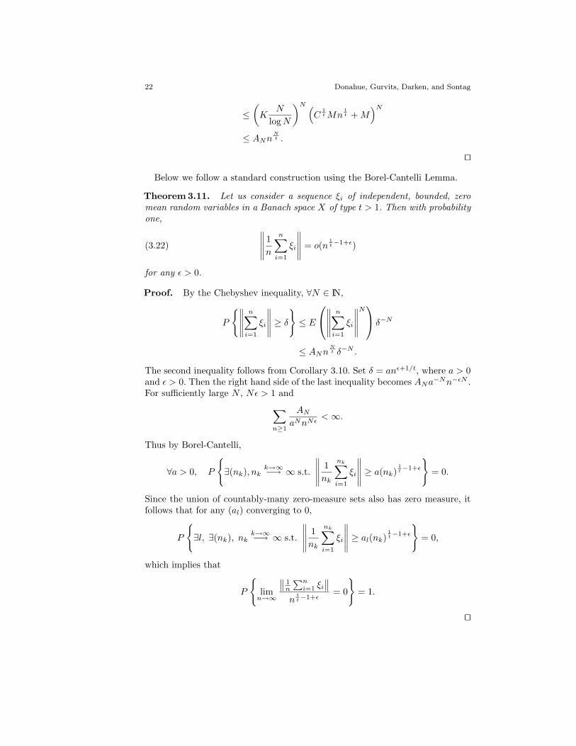
Below we follow a standard construction using the Borel-Cantelli Lemma.
Theorem 3.11. Let us consider a sequence ξi of independent, bounded, zeromean random variables in a Banach space X of type t > 1. Then with probabilityone,
∥
∥
∥
∥
∥
1
n
n∑
i=1
ξi
∥
∥
∥
∥
∥
= o(n1t−1+ǫ)(3.22)
for any ǫ > 0.
Proof. By the Chebyshev inequality, ∀N ∈ IN,
P
∥
∥
∥
∥
∥
n∑
i=1
ξi
∥
∥
∥
∥
∥
≥ δ
≤ E
∥
∥
∥
∥
∥
n∑
i=1
ξi
∥
∥
∥
∥
∥
N
δ−N
≤ ANnNt δ−N .
The second inequality follows from Corollary 3.10. Set δ = anǫ+1/t, where a > 0and ǫ > 0. Then the right hand side of the last inequality becomes ANa
−Nn−ǫN .For sufficiently large N , Nǫ > 1 and
∑
n≥1
AN
aNnNǫ<∞.
Thus by Borel-Cantelli,
∀a > 0, P
∃(nk), nkk→∞−→ ∞ s.t.
∥
∥
∥
∥
∥
1
nk
nk∑
i=1
ξi
∥
∥
∥
∥
∥
≥ a(nk)1t−1+ǫ
= 0.
Since the union of countably-many zero-measure sets also has zero measure, itfollows that for any (al) converging to 0,
P
∃l, ∃(nk), nkk→∞−→ ∞ s.t.
∥
∥
∥
∥
∥
1
nk
nk∑
i=1
ξi
∥
∥
∥
∥
∥
≥ al(nk)1t−1+ǫ
= 0,
which implies that
P
limn→∞
∥
∥
1n
∑ni=1 ξi
∥
∥
n1t−1+ǫ
= 0
= 1.
⊓⊔

Rates of Convex Approximation 23
We are now ready to investigate the GBS(φ) property. Suppose that f ∈coS ⊂ X. Then for any ǫ > 0 there exists a k(ǫ) < ∞ and gǫ
i ∈ S, αǫi > 0 for
1 ≤ i ≤ k(ǫ) with∑k(ǫ)
i=1 αǫi = 1 such that
∥
∥
∥
∥
∥
∥
f −k(ǫ)∑
i=1
αǫig
ǫi
∥
∥
∥
∥
∥
∥
< ǫ.
Let fǫ :=∑k(ǫ)
i=1 αǫig
ǫi , and consider a positive sequence (ǫn) such that
1
n
n∑
j=1
ǫj ≤ n1t−1.
Also select a sequence of independent random variables ξj such that Pξj =g
ǫj
i = αǫj
i for each i, 1 ≤ i ≤ k(ǫj). Then
∥
∥
∥
∥
∥
∥
1
n
n∑
j=1
ξj − f
∥
∥
∥
∥
∥
∥
=
∥
∥
∥
∥
∥
∥
1
n
n∑
j=1
(ξj − fǫj) − 1
n
n∑
j=1
(f − fǫj)
∥
∥
∥
∥
∥
∥
≤
∥
∥
∥
∥
∥
∥
1
n
n∑
j=1
ηj
∥
∥
∥
∥
∥
∥
+ n1t−1.
Here ηj = ξj − fǫj, so Eηj = 0. Applying Theorem 3.11 immediately yields:
Theorem 3.12. Any Banach space of type t, 1 < t ≤ 2, has the GBS(n1t−1+ǫ)
property for all ǫ > 0.
This can be restated as:
Corollary 3.13. Let X be a Banach space of type t, 1 < t ≤ 2, and let S be abounded subset of X with f ∈ coS. Then for all ǫ > 0, there exists a sequence(gi) ⊂ S such that the incremental sequence
fn =1
n
n∑
i=1
gi =n− 1
nfn−1 +
1
ngn(3.23)
satisfies
‖f − fn‖ = o(n1t−1+ǫ).(3.24)
Remark. The GBS(φ) property guarantees for f ∈ coS and S bounded theexistence of (gn) ⊂ S such that ‖f −∑n
i=1 gi/n‖ → 0. It is not true in generalthat one may pick all the gn distinct. Consider for example the Hilbert space ℓ2(which is of type 2, i.e., GBS(1/
√n)) and S = (en), where (en) is an orthonormal

24 Donahue, Gurvits, Darken, and Sontag
basis. Then coS =∑
i≥0 αiei where αi ≥ 0 and∑
αi = 1. But if enk6= enl
,(nk 6= nl) then
1
N
N∑
i=1
eni
‖·‖−→ 0.
However, it is possible to give necessary and sufficient conditions for the exis-tence of a sequence of distinct elements (gi) ⊂ S as above:
Theorem 3.14. Let X be a Banach space of type t, 1 < t ≤ 2, S ⊂ X,f ∈ coS. There exists a sequence (gi) ⊂ S where ∀i 6= j, gi 6= gj such that
‖∑ gi/n− f‖ → 0 if and only if for all finite K ⊂ S, f ∈ co(S \K).
Proof. That f ∈ co(S \K) for all finite K is sufficient follows from the discus-sion preceding Theorem 3.12. With this condition holding, we are free to choosethe g
ǫj
i to be distinct for all i and j.Necessity follows from considering a single finite-cardinality set K ⊂ S such
that f 6∈ co(S \K). Assume there exists a sequence of distinct elements (gi) ⊂ Ssuch that ‖f −
∑ni=1 gi/n‖ → 0. We will construct a sequence in co(S \ K)
converging to f , which is a contradiction.Since |K| < ∞ there must be an r > 0 such that ∀n > r, gn ∈ S \ K. Let
s > r. Then
fs :=1
s
s∑
i=1
gi =1
s
r∑
i=1
gi +1
s
s∑
i=r+1
gi.
As s→ ∞, the first sum tends to zero, so the second must tend to f . Thereforethe sequence
1
s− r
s∑
i=r+1
gi =s
s− r
1
s
s∑
i=r+1
gi
must also tend to f . Each element of this sequence is in co(S \K). ⊓⊔
4. Additional Assumptions on S
In the previous sections we have studied the convergence of convex approximatesfrom arbitrary bounded sets S as a function of the space X. However, it ispossible to improve the convergence behavior for a given space by imposingadditional assumptions on S. For example, suppose X = Lp(Ω) with 1 ≤ p < 2and m(Ω) < ∞. If there exists h ∈ L2(Ω) such that |g(x)| < h(x) for all x ∈ Ωand g ∈ S, then S ⊂ L2(Ω) as well, and the convex closure of S is the samein both Lp(Ω) and L2(Ω). Working in L2(Ω), we can find for each f ∈ coS anincremental sequence fn converging to f with rate O(1/
√n). This convergence
rate (with a different constant) then holds in Lp(Ω) as well, though in the latterspace the sequence might not be ǫ-greedy, especially in view of Theorem 3.1.

Rates of Convex Approximation 25
At the other end of the Lp spectrum, recall from Theorem 2.3 that there canbe no general rate bound in L∞. However, by restricting S to classes of indicatorfunctions, we can recover L2-like convergence in L∞. This approach, commonin the artificial neural network community, is especially interesting in patternclassification applications, and the connections with Vapnik-Chervonenkis (VC)dimension—first discovered by Barron in (Barron 1992)—are especially intrigu-ing.
In the following we adopt the convention of identifying an index (indicator)function with the set it indexes (i.e., its support), where the distinction is deter-mined by context.
Definition 4.1. Let F be a class of indicator functions on a set X. Let W bethe set of all Y ⊆ X such that for all Z ⊆ Y there exists an f ∈ F such thatf ∩ Y = Z. The “VC (Vapnik-Chervonenkis) dimension of F” is supY ∈W |Y |.
Our bounds (Theorem 4.5) are slightly weaker than those given by (Barron 1992)(ours are “big O” as compared to “little O”). However, the proof method hereseems worthy of note, especially as it makes use of more basic results than thecentral limit theorem relied upon in (Barron 1992).
We also explore the implications of good convergence rate bounds on the VCdimension of the corresponding set S. Good convergence rate bounds for S donot imply that S has a finite V C dimension (Theorem 4.6), i.e., the converse ofTheorem 4.5 is false. However, if any nontrivial rate bound holds uniformly forall subsets of S, its VC dimension must be finite (Theorem 4.7).
Definition 4.2. Let F be a class of indicator functions on a set X. Its dual F ′
is defined as the class evx, x ∈ X of indicator functions on F , where
evx(f) = f(x) ∀f ∈ F .
Thus, for each element ofX there is a unique element of F ′, named evx. Note thatit may be the case that evx = evy for x 6= y. One thinks of evx as the “evaluationat x operator” for elements of F . Note that evx contains the members of F whichcontain x.
Definition 4.3. Let V C be the operator on classes of indicator functions thatmeasures the Vapnik-Chervonenkis (VC) dimension. If F is a class of indicatorfunctions, we define the co-VC dimension by
coV C(F ) := V C(F ′).(4.25)
The next lemma is a consequence of (Ledoux and Talagrand 1991, Theo-rem 14.15, p. 418).
Lemma 4.4. Denote by M(Ω,Σ) the Banach space of all bounded signed mea-sures µ on (Ω,Σ) equipped with the norm ‖µ‖M := |µ|(Ω) ≡ µ+(Ω)+µ−(Ω). LetC ⊂ Σ; consider the operator j : M(Ω,Σ) → l∞(C) defined by j(µ) = (µ(c))c∈C .

26 Donahue, Gurvits, Darken, and Sontag
Then V C(C) < ∞ if and only if there exists a constant K such that for anyRademacher sequence γi and all finite sequences (µi) ⊂M(Ω,Σ),
E
∥
∥
∥
∥
∥
∑
i
γij(µi)
∥
∥
∥
∥
∥
sup
≤ K
(
∑
i
‖µi‖2M
)1/2
.(4.26)
If such a K exists, K = K ′√
V C(C), where K ′ is a universal constant.
Theorem 4.5. Let F be a class of indicator functions on a set X. Then F ⊂l∞(X). Let coV C(F ) = d < ∞. Then for any h ∈ coF , ‖conF − h‖sup ≤K(d/n)1/2, where K is a universal constant.
Proof. Since h ∈ coF , ∀ǫ > 0, ∃kǫ ∈ coF s.t. ‖h− kǫ‖sup < ǫ. We will neglectthe ǫ and write merely k where convenient. For some nǫ, kǫ =
∑nǫ
i=1 αifi, where∑nǫ
i=1 αi = 1, ai > 0, and fi ∈ F . Let Σk := σ(F ′ ∪ ∪nǫ
i=1fi). M(F,Σk) is aBanach space of bounded measures on F . The norm of µ ∈M(F,Σk) is ‖µ‖M =|µ|(F ) = µ+(F ) + µ−(F ). Define mi ∈ M(F,Σk) to be the probabilistic point-mass measure with support on fi, i.e., mi assigns measure 1 to sets containing fi
and 0 otherwise. Define µk :=∑n
i=1 αimi. Let ξl be finite-valued i.i.d. randomvariables taking value mi with probability αi. Define j : M(F,Σk) → l∞(X) byj(µ) := (µ(evx))x∈X . Note that j is a linear operator. By the triangle inequality,
Eξ
∥
∥
∥
∥
∥
j
(
n∑
i=1
ξl/n
)
− h
∥
∥
∥
∥
∥
sup
≤ Eξ
∥
∥
∥
∥
∥
j
(
∑
l
(ξl − µk)
)∥
∥
∥
∥
∥
sup
/n+ ‖h− k‖sup .
By a simple inequality (Ledoux and Talagrand, 1991, Lemma 6.3, p. 152),
Eξ
∥
∥
∥
∥
∥
∑
l
j (ξl − µk)
∥
∥
∥
∥
∥
sup
≤ 2EξEγ
∥
∥
∥
∥
∥
∑
l
γlj(ξl − µk)
∥
∥
∥
∥
∥
sup
,
where γl are i.i.d. random variables taking values +1 and -1 with equal proba-bility. Then by Lemma 4.4,
Eγ
∥
∥
∥
∥
∥
∑
l
γlj(ξl − µk)
∥
∥
∥
∥
∥
sup
≤ K√d
√
∑
l
‖ξl − µk‖2M .
Since ξl and µk are both probability measures, ‖ξl−µk‖M ≤ ‖ξl‖M +‖µk‖M = 2.Combining the above, we have
Eξ
∥
∥
∥
∥
∥
j
(
n∑
i=1
ξl/n
)
− h
∥
∥
∥
∥
∥
sup
≤ 4K√d√
n+ ǫ.
Since the inequality is true for all ǫ > 0 it remains true for ǫ = 0. Since for somerealization of the ξl the inequality must still hold, the theorem is proven. ⊓⊔

Rates of Convex Approximation 27
The mere fact of the existence of a convergence rate bound for a set of indicatorfunctions does not imply that the set has finite VC dimension. We give anexample to make this point.
Theorem 4.6. Let X be a measure space with an infinite number of measurablesets. Let S denote the set of indicator functions of all measurable sets. Clearly theVC dimension of S is infinite. However, if f ∈ coS, then f can be approximatedby an element of conS with error less than 1/n (in the uniform metric).
Proof. If f ∈ coS, then clearly 0 ≤ f(x) ≤ 1 for all x ∈ X. Fix n and define
Ak = f−1 ([(k − 1)/n, 1])
for k = 1, 2, . . . , n. (Note that some Ak may be empty.) Let gk be the indicatorfunction for Ak. Each gk is in S since f must be a measurable function. Thefunction
fn =
n∑
k=1
(1/n)gk
is in conS and satisfies
0 ≤ fn(x) − f(x) < 1/n
for all x ∈ X. (Moreover, this shows that coS equals the set of measurablefunctions with range in [0, 1].) ⊓⊔
However, if it is the case that one given convergence rate bound holds for allfinite subsets of a set of indicator functions, then the VC dimension of this setis finite.
Theorem 4.7. Let F be a set of indicator functions on a set X and C ⊆ F .Let α(C, r) be the worst-case rate of approximation of a member of the closedconvex hull of C by r elements of C. Assume that there is some function h sothat h(r) → 0 as r → ∞ such that α(C, r) ≤ h(r) for all finite C ⊂ F . ThenV C(F ) <∞.
Proof. We argue by contradiction. Assume that V C(F ) = ∞. Then alsocoV C(F ) = ∞. Thus, for each integer n there are elements x1, x2, . . . , x2n ∈ Xand functions f1, . . . , fn ∈ F such that (f1, . . . , fn) takes all 2n possible val-ues on these points. Define Cn := f1, . . . , fn. Consider approximating f :=∑n
i=1 fi/n ∈ coCn by r elements of Cn. By the symmetry of f , we can withoutloss of generality write the approximant as g =
∑ri=1 αifi. Then
‖g − f‖sup = supX
|g(x) − f(x)|
= supX
∣
∣
∣
∣
∣
r∑
i=1
(
αi −1
n
)
fi(x) −n∑
i=r+1
1
nfi(x)
∣
∣
∣
∣
∣
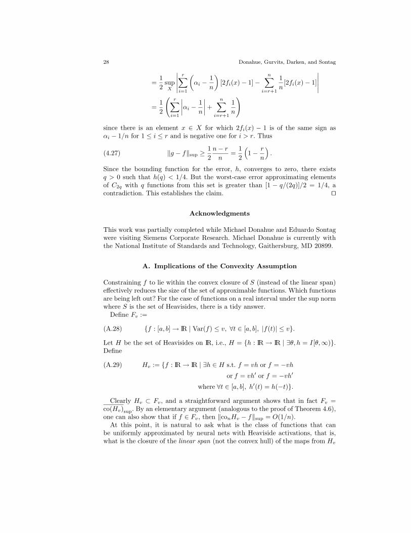
28 Donahue, Gurvits, Darken, and Sontag
=1
2supX
∣
∣
∣
∣
∣
r∑
i=1
(
αi −1
n
)
[2fi(x) − 1] −n∑
i=r+1
1
n[2fi(x) − 1]
∣
∣
∣
∣
∣
=1
2
(
r∑
i=1
∣
∣
∣
∣
αi −1
n
∣
∣
∣
∣
+
n∑
i=r+1
1
n
)
since there is an element x ∈ X for which 2fi(x) − 1 is of the same sign asαi − 1/n for 1 ≤ i ≤ r and is negative one for i > r. Thus
‖g − f‖sup ≥ 1
2
n− r
n=
1
2
(
1 − r
n
)
.(4.27)
Since the bounding function for the error, h, converges to zero, there existsq > 0 such that h(q) < 1/4. But the worst-case error approximating elementsof C2q with q functions from this set is greater than [1 − q/(2q)]/2 = 1/4, acontradiction. This establishes the claim. ⊓⊔
Acknowledgments
This work was partially completed while Michael Donahue and Eduardo Sontagwere visiting Siemens Corporate Research. Michael Donahue is currently withthe National Institute of Standards and Technology, Gaithersburg, MD 20899.
A. Implications of the Convexity Assumption
Constraining f to lie within the convex closure of S (instead of the linear span)effectively reduces the size of the set of approximable functions. Which functionsare being left out? For the case of functions on a real interval under the sup normwhere S is the set of Heavisides, there is a tidy answer.
Define Fv :=
f : [a, b] → IR | Var(f) ≤ v, ∀t ∈ [a, b], |f(t)| ≤ v.(A.28)
Let H be the set of Heavisides on IR, i.e., H = h : IR → IR | ∃θ, h = I[θ,∞).Define
Hv := f : IR → IR | ∃h ∈ H s.t. f = vh or f = −vh(A.29)
or f = vh′ or f = −vh′
where ∀t ∈ [a, b], h′(t) = h(−t).
Clearly Hv ⊂ Fv, and a straightforward argument shows that in fact Fv =co(Hv)sup. By an elementary argument (analogous to the proof of Theorem 4.6),one can also show that if f ∈ Fv, then ‖conHv − f‖sup = O(1/n).
At this point, it is natural to ask what is the class of functions that canbe uniformly approximated by neural nets with Heaviside activations, that is,what is the closure of the linear span (not the convex hull) of the maps from Hv
Rates of Convex Approximation 29
(which is the same for all v of course). This is a classical question; see for instance(Dieudonne 1960, VII.6): the closure is the set of all regulated functions, thatis, the set of functions f : [a, b] → R for which limx→x−
0
f(x) and limx→x+
0
f(x)
exist for all x0 ∈ [a, b) and x0 ∈ (a, b], respectively. Thus, by constraining targetfunctions to the convex closure ofHv instead of the span, we are losing the abilityto approximate those regulated functions that are not of bounded variation.
In the multivariable case, that is, f : K → IR with K a compact subset ofIRn, the situation is far less clear. If f has “bounded variation with respect tohalf-spaces” (i.e., is in the convex hull of the set of all half spaces (Barron 1992)),and in particular if f admits a Fourier representation
f(x) =
∫
IRn
ei〈ω,x〉f(ω)dω
with∫
IRn
‖ω‖|f(ω)|dω <∞,
then by (Barron 1992) there are approximations with rate O(1/√n) (since f
is in the convex hull of the Heavisides). But the precise analog of regulatedfunctions is less obvious. One might expect that piecewise constant functionscan be uniformly approximated, for instance, at least if defined on polyhedralpartitions, but this is false.
For a counterexample, let f be the characteristic function of the square [−1, 1]2
in IR2, and let K be, for instance, a disc of radius 2 centered on (0, 0). Thenit is impossible to approximate f to within error 1/8 by a one hidden-layerneural net, that is, a linear combination of terms of the form H(〈w, x〉+ b), withw ∈ IR2 and b ∈ IR. (Constant terms on K can be included, without loss ofgenerality, by choosing b appropriately.) This is proved as follows. If there wouldexist a function g of this form, that approximates to within 1/8, then close tothe boundary of the disc its values are in the range (−1/8, 1/8), and near thecenter of the square it has values > 7/8. Moreover, everywhere the values ofg are in (−1/8, 1/8)
⋃
(7/8,+∞). Now, the function 4g − (1/2) is again in thesame span, and it now has values in (−1, 0) and (3,+∞) in the same regions.This contradicts (Sontag 1992, Prop. 3.8). (Of course, one can also prove thisdirectly.)
B. Properties of the Modulus of Smoothness
In this section we collect some inequalities related to power type estimates ofthe modulus of smoothness. In particular, the first lemma shows that Lp spacesare of power type t = min(p, 2). (See Corollary 3.6 and Theorem 3.7.)
Lemma B.1. If X = Lp, 1 ≤ p < ∞, then the modulus of smoothness ρ(u)satisfies
ρ(u) ≤
up/p if 1 ≤ p ≤ 2(p− 1)u2/2 if 2 ≤ p <∞(B.30)
30 Donahue, Gurvits, Darken, and Sontag
for all u ≥ 0.
Proof. From the definition of the modulus of smoothness we have
2(ρ(u) + 1) = sup‖f + g‖ + ‖f − g‖ | ‖f‖ = 1, ‖g‖ = u≤ 21/q sup(‖f + g‖p + ‖f − g‖p)
1/p | ‖f‖ = 1, ‖g‖ = u,(B.31)
where q = p/(p − 1). The inequality follows from the concavity of the functiont→ t1/p. Next we make use of some inequalities given by Hanner (1956):
(‖f‖ + ‖g‖)p + | ‖f‖ − ‖g‖ |p ≤ ‖f + g‖p + ‖f − g‖p(B.32)
≤ 2(‖f‖p + ‖g‖p),
for 1 < p ≤ 2. The inequalities hold in the reverse sense if 2 ≤ p < ∞. (Thesecond inequality above is actually due to Clarkson (1936).) Combining this with(B.31) yields
ρ(u) ≤
(1 + up)1/p − 1 if 1 ≤ p ≤ 2[
(1 + u)p + |1 − u|p2
]1/p
− 1 if 2 ≤ p <∞(B.33)
This result is cited in (Lindenstrauss 1963). It is possible to use the methods in(Hanner 1956) to show that the above bounds on ρ(u) are tight.
For 1 < p ≤ 2, (B.30) now follows immediately. For p ≥ 2 and 0 ≤ u ≤ 1 aTaylor series expansion shows
(
(1 + u)p + (1 − u)p
2
)1/p
≤ p− 1
2u2 + 1,(B.34)
which proves (B.30) for 2 ≤ p < ∞ and 0 ≤ u ≤ 1. For u > 1, divide by u anduse (B.34) again:
(
(u+ 1)p + (u− 1)p
2
)1/p
= u
(
(1 + 1/u)p + (1 − 1/u)p
2
)1/p
≤ u+p− 1
2u
≤ p− 1
2u2 + 1,
for 2 ≤ p <∞ and u > 1. ⊓⊔
For completeness we note the following result, the proof of which is left to thereader.
Theorem B.2. Let X be a Banach space. The modulus of smoothness for Xsatisfies
ρ(u) ≤ u for all u ≥ 0.(B.35)
Furthermore, if X is L1 or L∞ with dimension at least 2, then
ρ(u) = u for all u ≥ 0.(B.36)

Rates of Convex Approximation 31
The following technical lemma uses an inequality of Lindenstrauss to pro-vide several lower bounds on γ as a function of t for spaces with modulus ofsmoothness ρ(u) ≤ γut. These are needed in Theorem 3.5.
Lemma B.3. Let X be a Banach space with modulus of smoothness ρ(u) sat-isfying ρ(u) ≤ γut for all u ≥ 0. Then 1 ≤ t ≤ 2 and
γt ≥
[(2 − t)t]1−t/2
(t− 1)t−1 if 1 < t < 21 if t = 1 or t = 2.
(B.37)
Moreover, for all t ∈ [1, 2],
γ ≥√
2 − 1,(B.38)
γ ≥ 3−t/2,(B.39)
γ ≥ 2t−1/5t/2,(B.40)
γ >1
te−3/2e.(B.41)
Proof. Lindenstrauss (1963) gives√
1 + u2 − 1 ≤ ρ(u) ≤ γut for all u ≥ 0.(B.42)
Letting u→ ∞ shows that t ≥ 1, and if t = 1 then γ ≥ 1. Furthermore,
γut ≥√
1 + u2 − 1 ≥ u2
2 + u2,
so letting u ↓ 0 proves that t ≤ 2 and if t = 2 then γ ≥ 1/2.Therefore t satisfies 1 ≤ t ≤ 2, and inequalities (B.37) through (B.41) hold if
t = 1 or t = 2. Next assume 1 < t < 2, and rewrite (B.42) as
γ ≥√
1 + u2 − 1
utfor all u ≥ 0.
In particular, this inequality holds if we replace u with√
(2 − t)t/(t− 1), whichgives
γ ≥ (2 − t)1−t/2(t− 1)t−1
tt/2.(B.43)
This completes the proof of (B.37).Inequality (B.38) follows from (B.42) by setting u = 1. Using u =
√3 provides
(B.39), and (B.40) is obtained with u =√
5/2.To prove (B.41), place the inequality xx ≥ e−1/e into (B.43) to obtain
γ ≥ t−t/2e−1/2ee−1/e.
Then use 1 < t < 2 to complete the proof. ⊓⊔
These estimates are compared in Figure 2.

32 Donahue, Gurvits, Darken, and Sontag
1
te−3/2e
2t−1/5t/2
3−t/2
√2 − 1
1
t[(2 − t)t]1−t/2(t − 1)t−1
2.01.81.61.41.21.0
1.0
0.8
0.6
0.4
0.2
0.0
Fig. 2. Comparison of lower bound estimates on γ (from Lemma B.3) as a function of t.
Lemma B.4. Let ρ(u) be the modulus of smoothness of a Banach space, andassume that ρ(u) ≤ γut for all u ≥ 0 (t ∈ [1, 2] is fixed). Then
1 +1
(2γ)1/t<
(
5t− 1
2
)1/t
.(B.44)
Proof. Define h(t) to be the right-hand side of (B.44). Then the derivative ofh(t) has the same sign as
5t− 1
2
(
1 − log
(
5t− 1
2
))
+1
2.(B.45)
But (B.45) is decreasing in t for t > 3/5, so h′(t) = 0 for at most one pointt0 ∈ [1, 2] (in fact t0 ≈ 1.4724), which would be a local maximum for h. Inparticular, for any subinterval [t1, t2] ⊂ [1, 2], it must be that
h(t) ≥ min (h(t1), h(t2)) for all t ∈ [t1, t2].
For our purposes we divide the interval [1, 2] into two subintervals: [1, 5/4] and[5/4, 2]. Evaluating h at the endpoints yields
h(1) = 2
h(5/4) = (21/8)4/5 > 2.16
h(2) = 3/√
2 > 2.12.

Rates of Convex Approximation 33
Therefore h(t) ≥ 2 for t ∈ [1, 5/4], and h(t) ≥ 2.12 for t ∈ [5/4, 2].To obtain the corresponding upper bounds on the left-hand side of (B.44),
apply (B.39) for t ∈ [1, 5/4], and (B.40) for t ∈ [5/4, 2]. ⊓⊔
C. A Sequence Inequality
The following lemma may be viewed as pertaining to a discrete analogue of thedifferential equation y′ = y1−t, the general solution of which is y(x) = (tx+C)1/t.It can be used to provide bounds on the convergence rate of sequences havingincremental changes compatible with the estimates from Lemma 3.3, with whichit is combined to produce Theorems 3.5 and 3.7.
Lemma C.1. Let (an) be a nonnegative sequence satisfying
an+1 ≤ an + min
(
3
2,
1
at−1n
)
(C.46)
for all n, where 1 ≤ t ≤ 2. If
an ≤(
tn+t− 1
2log2 n
)1/t
(C.47)
is satisfied for some n ≥ 2, or for n = 1 with a1 ≥ 1, then it is satisfied for alln′ > n as well.
Proof. Let us take bn := tn + (1/2)(t − 1) log2 n, assume that an ≤ b1/tn , and
proceed by induction, i.e., show that an+1 ≤ b1/tn+1.
Suppose first that an < 1 and n ≥ 2. Then
b1/tn+1 ≥ b
1/t3 ≥ (6 + (1/2) log2 3)1/2 > 5/2.
The second inequality holds because the function t 7→ (3t+(1/2)(t−1) log2 3)1/t
is decreasing in t for t ∈ [1, 2], and so attains its minimum at t = 2. But then
an+1 ≤ an + 3/2 < 5/2 < b1/tn+1,
as desired.Alternatively, suppose that an ≥ 1. Then since the function x 7→ x(1 + 1/xt)
is nondecreasing for x ≥ 1, we have
an+1 ≤ an(1 + 1/atn) ≤ b1/t
n (1 + 1/bn)
≤ b1/tn
[
1 +t
bn+t(t− 1)
2b2n
]1/t
≤[
t(n+ 1) +t− 1
2log2(n+ 1) +
t− 1
2n− t− 1
2log2(1 + 1/n)
]1/t
.
34 Donahue, Gurvits, Darken, and Sontag
The third inequality above follows from a Taylor series expansion of (1+1/bn)t.Combining this with the definition of bn+1 and the fact that log2(1+1/n) ≥ 1/nfor n ≥ 1 yields
an+1 ≤ b1/tn+1,
concluding the proof. ⊓⊔
D. An Example of a Smooth Banach Space with Non-Convergingǫ-Greedy Sequences
In Sect. 3.1 it was shown that ǫ-greedy sequences in uniformly smooth spacesalways converge (provided
∑
ǫk < ∞), and that smoothness is necessary andsufficient for monotonically decreasing error in incremental approximants. Wenow construct an example showing that simple smoothness is insufficient toguarantee convergence of ǫ-greedy sequences.
Let a = (a(n)) be a sequence of real numbers. Define the sequence of functions(Fn) (the norm sequence) from IRIN to IR+ ∪ 0 recursively by
F1(a) = |a(1)|Fn(a) = [(Fn−1(a))
pn + |a(n)|pn ]1/pn ,
where (pn) is a fixed sequence (called the norm power sequence) with 1 ≤ pn <∞for all n.
Note that for each a, Fn(a) is nondecreasing with n. Define
X(pn) :=
a ∈ IRIN | supnFn(a) <∞
,(D.48)
and for a ∈ X(pn)
‖a‖ := F (a) := limn→∞
Fn(a).(D.49)
The reader may verify that X(pn) equipped with the norm (D.49) is a Banachspace. (This space is similar to the modular sequence spaces studied in (Woo1973).) If (pn) is bounded and pn > 1 for all n, then it can be shown that X(pn)
is smooth. Let us use the notation en ∈ X(pn) to denote the canonical basiselement en(k) = δn(k). (Note that ‖en‖ = 1 for all n independent of (pn).)
Proposition D.1. Let (γn) be a strictly decreasing sequence converging to 1.Then there exists a norm power sequence (pn) that is non-increasing, convergesto 1, and has pn > 1 for all n, such that the bounded set S = −γ1e1 ∪γnenn∈IN in X(pn) admits for each incremental schedule (ǫn) an incrementalsequence (an) ⊂ coS that is ǫ-greedy with respect to 0 but does not converge.(Note that 0 ∈ coS.)

Rates of Convex Approximation 35
Proof. X(pn) is determined by its power sequence (pn). Choose p1 > 1 arbi-trarily, and recursively select pn ∈ (1, pn−1] to satisfy
inf0≤λ≤1
[(1 − λ)γn−1]pn + (λγn)pn > 1.(D.50)
This can always be done because the inequality holds for pn = 1 and so bycontinuity in pn holds also for all pn sufficiently close to 1.
Now let (ǫk) be a fixed incremental schedule. We build an ǫ-greedy (withrespect to 0) sequence (ak) ⊂ S ⊂ coS as follows. Let a1 = γn1
en1be any ǫ1-
greedy element of S with n1 > 1 (i.e., γn1< min1 + ǫ1, γ1). Assuming that
ak−1 = γnk−1enk−1
with nk−1 > 1, we will show that we can pick ak = γnkenk
with nk > nk−1 to be ǫk-greedy. Indeed, suppose that
bk = (1 − λ)ak−1 + λgk
is an ǫk-greedy step, where gk ∈ S. It follows from (D.50) and the monotonicityof γn that ‖bk‖ > 1, so we can pick nk > nk−1 such that
‖bk‖ > γnk= ‖γnk
enk‖.
Therefore, taking ak = γnkenk
yields an ǫk-greedy increment.We define the sequence (ak) recursively in this manner to complete the con-
struction. ⊓⊔
References
Banach, S., and S. Saks (1930) Sur la convergence forte dans les champs LP , Studia Math.,2:51–57.
Barron, A. R. (1991) Approximation and estimation bounds for artificial neural networks, in
Proc. Fourth Annual Workshop on Computational Learning Theory, Morgan Kaufmann,243–249.
Barron, A. R. (1992) Neural net approximation, in Proc. of the Seventh Yale Workshop on
Adaptive and Learning Systems, 69–72.Bessaga, C., and A. Pelczynski (1958) A generalization of results of R. C. James concerning
absolute bases in Banach spaces, Studia Math., 17:151–164.Clarkson, J. A. (1936) Uniformly convex spaces, Trans. Amer. Math. Soc., 40:396–414.
Darken, C., M. Donahue, L. Gurvits, and E. Sontag (1993) Rate of approximation results mo-tivated by robust neural network learning, in Proc. of the Sixth Annual ACM Conferenceon Computational Learning Theory, The Association for Computing Machinery, New York,
N.Y. 303–309.Deville, R., G. Godefroy, and V. Zizler (1993) Smoothness and Renormings in Banach Spaces.
Wiley, N.Y..Dieudonne, J. (1960) Foundations of Modern Analysis. Academic Press, N.Y..
Figiel, T. and G. Pisier (1974) Series aleatoires dans les espaces uniformement convexes ouuniformement lisses, C. R. Acad. Sci. Paris, 279, Serie A:611–614.
Gowers, W. T., A Banach space not containing c0, l1, or a reflexive subspace. Preprint.Haagerup, U. (1982) The best constants in the Khintchine inequality, Studia Math., 70:231–
283.Hanner, O. (1956) On the uniform convexity of Lp and ℓp, Arkiv for Matematik, 3:239–244.Hanson, S. J. and D. J. Burr (1988) Minkowski-r back-propagation: learning in connection-
ist models with non-Euclidean error signals, in Neural Information Processing Systems,American Institute of Physics, New York, 348.

36 Donahue, Gurvits, Darken, and Sontag
James, R. C. (1978) Nonreflexive spaces of type 2, Israel J. Math., 30 :1–13.Jones, L. K. (1992) A simple lemma on greedy approximation in Hilbert space and convergence
rates for projection pursuit regression and neural network training, Annals of Statistics,20:608–613.
Kakutani, S. (1938) Weak convergence in uniformly convex spaces, Tohoku Math. J., 45:188–193.
Khintchine, J. (1923) Uber die diadischen Bruche. Math. Z., 18:109-116.Ledoux, M. and M. Talagrand (1991) Probability in Banach Space. Springer-Verlag, Berlin.Leshno, M., V. Lin, A. Pinkus, and S. Schocken (1992) Multilayer feedforward networks with
a non-polynomial activation function can approximate any function. Preprint. Hebrew Uni-versity.
Lindenstrauss, J. (1963) On the modulus of smoothness and divergent series in Banach spaces,The Michigan Math. J., 10:241–252.
Lindenstrauss, J. and L. Tzafriri (1979) Classical Banach Spaces II: Function Spaces. Springer-Verlag, Berlin.
Powell, M. J. D. (1981) Approximation theory and methods. Cambridge University Press,
Cambridge.Rey, W. J. (1983) Introduction to Robust and Quasi-Robust Statistical Methods. Springer-
Verlag, Berlin.Rosenthal, H. (1974) A characterization of Banach spaces containing l1, Proc. Nat. Acad. Sci.
(USA), 71:2411–2413.Rosenthal, H. (1994) A subsequence principle characterizing Banach spaces containing c0, Bull.
Amer. Math. Soc., 30:227–233.Sontag, E. D. (1992) Feedback stabilization using two-hidden-layer nets, IEEE Trans. Neural
Networks, 3:981–990.Stromberg, K. R. (1981) An Introduction to Classical Real Analysis. Wadsworth, New York.Woo, J. Y. T. (1973) On modular sequence spaces, Studia Math., 48:271–289.
Michael J. DonahueInstitute for Mathematics and its ApplicationsUniversity of MinnesotaMinneapolis, MN 55455
Leonid GurvitsNEC Research Institute4 Independence WayPrinceton, NJ 08540
Christian DarkenLearning Systems DepartmentSiemens Corporate Research, Inc.755 College Road EastPrinceton, NJ 08540
Eduardo SontagDepartment of MathematicsRutgers UniversityNew Brunswick, NJ 08903
This article was processed using the LATEX macro package with CAP style