rational gudiance to determine the maximum factored …docs.trb.org/prp/17-05334.pdf · rational...

Abu-Hejleh, N., Kramer, W.M., Mohamed, K., Long, J.H., and Zaheer, M 1

RATIONAL GUDIANCE TO DETERMINE THE MAXIMUM FACTORED AXIAL COMPRESSION LOAD A DRIVEN PILE CAN SUPPORT

By:

Naser M. Abu-Hejleh, Ph.D., P.E (Corresponding Author) Geotechnical Engineering Specialist

FHWA Resource Center 4749 Lincoln Mall Drive, Suite 600, Matteson, IL 60443

Ph. 708-283-3550; Fax: 708 283 3550; E-mail: [email protected]

William Kramer, P.E. Foundations and Geotechnical Unit Chief

Bureau of Bridges and Structures, Illinois Department of Transportation Ph. (217) 782-7773, E-mail: [email protected]

Khalid Mohamed, PE., PMP

Principal Bridge Engineer - Geotechnical FHWA Headquarter, Washington, DC

Ph: 202-366-0886; Email: [email protected]

James H. Long Emeritus Faculty

Department of Civil Engineering, University of Illinois (217) 333-2543; E-mail: [email protected]

Mir A. Zaheer, P.E.

Geotechnical Design Engineer Office of Geotechnical Services, Indiana Department of Transportation

Ph. (317) 610 7251 Ext. 224; E-mail: [email protected]

Submitted to: 94th th Transportation Research Board Annual Meeting

Washington, D.C.

No. of text words = 5650 No. of figures and tables (6) x 250 words/Figure = 1500

Total number of words = 7150

mailto:[email protected]

mailto:[email protected]


ABSTRACT 1 2 FHWA developed publications that address several issues and problems that highway agencies 3 face in implementing LRFD design for driven piles based on AASHTO LRFD Bridge Design 4 Specifications. Initially in this paper, new improvements for consideration of downdrag effects in 5 the design of driven piles are presented followed by discussion of how these improvements 6 impact the design procedure for driven piles presented in previous FHWA publications. The 7 maximum factored axial compression load a driven pile can support at the strength limit state 8 (Qfmax) is needed to start the design and estimate the preliminary number of piles in a pile group 9 and finalize the design. Procedure to estimate Qfmax is not discussed in AASHTO LRFD. The 10 current common practices used by highway agencies to determine Qfmax are conservative and 11 require lengthy design time. To address these problems, a new rational guidance to determine 12 Qfmax at the beginning of the design is presented. Qfmax is determined by addressing all the 13 strength limit states for compression resistance of a single pile, geotechnical, drivability, and 14 structural. A new and improved procedure is developed to address pile drivability in the design 15 by determining the maximum depth (length) the pile can be safely driven to without damage, 16 Lmax. The results obtained from addressing all the strength limit states for compression resistance 17 of a driven pile are summarized in a design chart that can be used to optimize and finalize the 18 design. Finally, a comprehensive LRFD Design Example is solved to demonstrate the driven pile 19 design guidance presented in this paper. The benefits of setup and using static load tests are also 20 demonstrated in solving this example. 21 22 23


INTRODUCTION 1 2 The FHWA recently developed a new NHI training Course Number 132083, “Implementation 3 of LRFD Geotechnical Design for Bridge Foundations” (1). The goal of this course is to assist 4 State Departments of Transportation (DOTs) in the successful development of LRFD design 5 specifications for bridge foundations based on AASHTO LRFD Bridge Design Specifications (2) 6 and their local experiences. Majority of the LRFD implementation issues received by FHWA 7 from the State DOTs are related to the LRFD design of driven piles. These issues are identified 8 and addressed in another FHWA LRFD implementation publication (3), titled “Implementation 9 of AASHTO LRFD Design Specifications for Driven Piles.” 10 11 The geotechnical strength limit state for compression resistance of a single pile is used to 12 determine the pile length or depth, L, needed to support a given load Qf, defined as the largest 13 factored axial compression load applied to the top of a single pile in a pile group. Addressing this 14 limit state requires the pile nominal bearing resistances of a single pile, Rn, at various depths. In 15 AASHTO Article 10.7.3.8 (2), two types of methods are used to determine the pile nominal 16 bearing resistances and the pile length (depth): 17 • The static analysis methods (e.g., α-method). According to AASHTO, the static analysis 18

methods are commonly used for estimating pile quantities in the design phase and may be 19 used to finalize pile length in certain cases where field analysis methods are unsuitable. 20 According to the FHWA LRFD Implementation Manual (Abu-Hejleh et. al., 2010), the static 21 analysis methods can be used in all cases to finalize the pile length as long as site variability 22 is addressed in the design. Use and advantages of static analysis methods to finalize pile 23 length in the design phase are discussed by Abu-Hejleh et. al. (3, 4) and will not be covered 24 in this paper. 25

• The field analysis methods. These include the static load test and the following dynamic 26 analysis methods: dynamic testing with signal matching, wave equation analysis, and 27 dynamic formulas. The dynamic analysis methods have two main components: an analytical 28 model and driving information obtained in the field during driving the pile, like the pile 29 penetration resistance, driving stresses, and the hammer developed energy and efficiency. 30 The field analysis methods are routinely used by the vast majority of State DOTs to verify 31 pile bearing resistances and finalize the pile length in the field during construction (often 32 using test piles). As will be discussed later, addressing the geotechnical strength limit state 33 with these methods will lead to two design outputs: 34 • The required nominal bearing resistance needed to determine pile length in the field 35

(AASHTO LRFD Articles 10.7.3.8, 10.7.7, and 10.7.9). The strength limit state must be 36 met in the field by driving the pile to a depth where the required nominal bearing 37 resistance is achieved or exceeded. 38

• An estimate of the pile length, L, needed to achieve the required bearing resistance 39 (Article 10.7.3.3). This length, often estimated in the design phase using the static 40 analysis methods, may be different from the final length determined in the field 41 (discussed in the previous item). Abu-Hejleh et al. (3, 4) described a new procedure to 42 improve the agreement between this length, L, and pile length finalized in the field during 43 construction. 44

45


Initially, new improvements for consideration of downdrag effects in the design of driven piles 1 are presented followed by discussion of how these improvements impact the design procedures 2 for driven piles presented in previous FHWA publications (1, 3, and 4). 3 4 The maximum factored axial compression load a driven pile can support (Qfmax) at the strength 5 limit state is needed to estimate the preliminary number of piles in a pile group. This would 6 allow for estimation of Qf and the pile length, L, needed to support Qf based on the geotechnical 7 strength limit as discussed before. Once the preliminary layout of a pile group is established 8 (number, depth, and location of piles), all other LRFD limit states can be checked and the final 9 layout of the pile group that meet all LRFD limit states can be developed. Procedure to 10 determine Qfmax is not discussed in AASHTO LRFD (2). The current common practices used by 11 highway agencies to develop initial Qfmax are based on the structural capacity of the pile. If pile 12 drivability is not met with this initial Qfmax, the value of Qfmax is reduced until drivability is met. 13 In this procedure, the impact of using better geotechnical design methods (e.g., load tests) or 14 setup in determining Qfmax is not considered. Therefore, the current common practices used by 15 highway agencies to determine Qfmax are conservative and require lengthy design time. 16 17 To address the above problems, this paper presents a new rational guidance to determine Qfmax at 18 the beginning of the design, which would shorten design time and allow for design optimizing 19 from the beginning stages of design. Qfmax is determined by addressing all the strength limit 20 states for compression resistance of a single pile, geotechnical, drivability, and structural. A new 21 and improved procedure is developed to address pile drivability by determining the maximum 22 length the pile can be safely driven to without damage, Lmax. Then, Lmax is used to determine 23 Qfmax and address drivability of pile lengths developed in the design to address all applicable 24 LRFD limit states (not only strength limit state). The results obtained from addressing all the 25 strength limit states for compression resistance of a driven pile are summarized in a design chart 26 that can be used to optimize and finalize the design. Finally, a comprehensive LRFD Design 27 Example is solved to demonstrate the driven pile design guidance presented in this paper. The 28 benefits of setup and using static load tests are also demonstrated in solving this example. 29 30 EFFECTS OF DOWNDRAG ON THE LRFD DESIGN OF DRIVEN PILES 31 32 According to the AASHTO LRFD (2), downdrag causes two effects on piles: an additional 33 compression axial load and an additional lost geotechnical resistance (AASHTO Articles 3.11.8, 34 10.7.1.6.2, and 10.7.3.7). The factored downdrag load is γpDD, where DD is the downdrag load, 35 and γp is its load factor. AASHTO LRFD considers both these effects in the geotechnical strength 36 limit state analysis of driven piles. This AAASHTO approach was adopted in the previous 37 publications (1, 3, and 4). But the new FHWA manual on driven piles (5) presents new changes 38 and improvements for consideration of downdrag effects in the design of driven piles presented 39 next for two typical pile cases: 40 • A single driven pile seated on top of hard rock. In this case, settlement of the pile is very 41

small and could be less that settlement of the downdrag soil layer, so downdrag effect could 42 be mobilized at all limit states. Also, in this case, the pile axial structural compression 43 resistance, Pn, is less the pile nominal bearing (geotechnical) resistance, Rn, and will control 44 Qfmax that can be computed as φstr Pn - γp DD, where φstr is the pile structural resistance factor 45 discussed in AASHTO LRFD Sections 5, 6, and 7 (2) for various types of pile materials. 46


• A single pile driven in soils or soft rocks. In this case, as the pile head axial compression 1 load approaches the nominal bearing geotechnical resistance for the geotechnical strength limit 2 state, the settlement of the pile will exceed settlement of the downdrag soil layer, causing the 3 effect of downdrag to disappear at that limit state. Hence, downdrag should not be considered at 4 the geotechnical strength limit state for compression resistance of a single pile. But the two 5 effects of downdrag discussed above should be considered at the service limit state for 6 settlement. 7

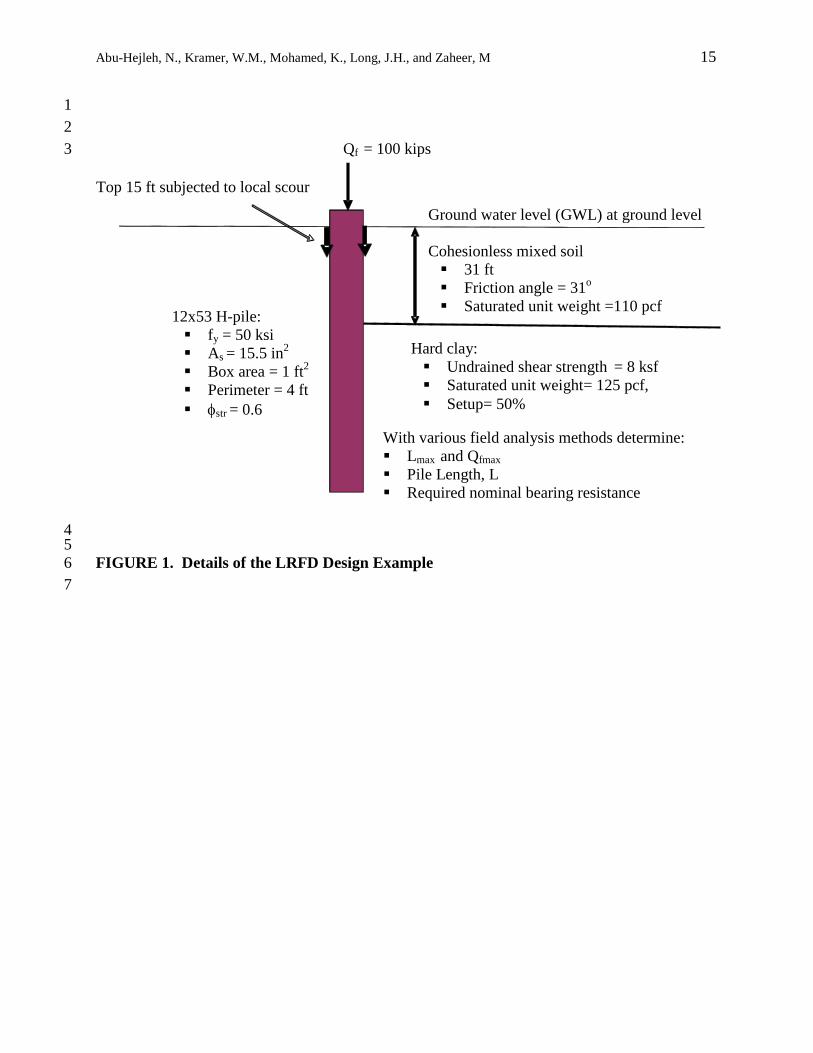
8 Subsequent sections of this paper deal with piles driven in soils or soft rocks, where Qfmax is 9 determined by addressing all the strength limit states for compression resistance of a single pile 10 (geotechnical, drivability, and structural) without including any effect from downdrag. This will 11 correct the procedures presented before (1, 3, and 4) where the two downdrag effects discussed 12 above were considered at the structural and geotechnical strength limit states. 13 14 LRFD DESIGN EXAMPLE 15 16 To demonstrate the LRFD design procedure presented in subsequent sections of this paper, an 17 example problem is developed and a step by step solution is presented. Figure 1 illustrates the 18 details of this example. There are two soil layers: cohesionless mixed soil with no setup that 19 extends to a depth of 31 ft from the ground surface, underlain by hard overconsolidated clay with 20 an estimated setup factor of 50 percent (%). The top 15 ft of the loose silty sand layer will be 21 subjected to local scour. The pile type is a 12x53 H-pile with steel yield strength, fy, of 50 ksi, 22 steel area, As, of 15.5 in2, box area of 1 ft2, box perimeter of 4 ft, and a structural resistance 23 factor, φstr, of 0.6 selected based on AASHTO LRFD Article 6.5.4.2 (2) for good (easy) driving 24 conditions expected herein. 25 26 It is required to develop design charts for the driven pile using the following three AASHTO 27 LRFD (2) field analysis methods: 28

1. Wave equation analysis at end of driving (EOD) conditions with φ =0.5 (no dynamic 29 measurements) 30

2. Wave equation analysis at beginning of restrike (BOR) conditions with φ =0.5 (no 31 dynamic measurements) 32

3. Axial compression static load test, with φ = 0.8. In addition to the static load test, dynamic 33 testing of at least two piles per site conditions, but no less than 2% of the production piles, 34 will be performed. 35 36

It is also required to use the developed design charts to: i) develop Qfmax, and ii) determine the 37 pile lengths, L, and field nominal bearing resistances required to support Qf= 100 kips. 38 39 GEOTECHNICAL STRENGTH LIMIT STATE FOR COMPRESSION RESISTANCE 40 OF A SINGLE DRIVEN PILE 41 42 This limit state was thoroughly discussed in FHWA report (3) and the 2015 TRB paper (4). It 43 will be briefly described in this section to the extent needed to show the procedure to determine 44 Qfmax and achieve other goals of this paper. 45 46


Types of Pile Nominal Bearing Resistances: 1 2 • Driving Resistance, Rndr. It is the resistance mobilized during pile driving until the end of 3

driving (EOD), Rndr. 4 • Short-term resistance, Rnre. This is the resistance that is developed shortly after pile driving. 5

It includes the permanent changes in the pile’s geotechnical resistances that occur after EOD, 6 for example due to setup and relaxation. Soil setup, expressed as a percentage, is defined as 7 100(Rnre – Rndr)/Rndr. 8

• Long-term resistance (Rn). It is defined as the minimum pile bearing resistance that would 9 always be available to support the applied loads during the entire design life of the 10 foundation. It does not include the geotechnical resistance losses (GL) that may not be 11 available during the foundation design life, for example from scour, and future increases of 12 the groundwater level (GWL) after pile driving. 13

14 Governing Equation 15 16 The governing equation for the geotechnical strength limit state is: 17

18 Qf ≤ φ Rn (1) 19

20 Where φ is the geotechnical resistance factor for the method employed to determine Rn. For 21 static analysis methods Rn = Rnstat and φ = φstat and for field analysis methods, Rn = Rnfield and φ = 22 φdyn. In Eq. 1, the downdrag effects are not considered but were considered in similar equation 23 presented in previous publications (3 and 4). 24 25 Bearing Resistances from Static Analysis Methods 26

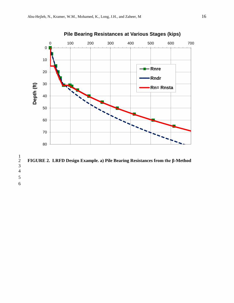
27 Abu-Hejleh et. al. (3, 4) discussed the determination of the bearing resistances from static 28 analysis methods. 29 30 To solve the LRFD example, Abu-Hejleh et. al. (3, 4) selected the β-method to develop the static 31 analysis pile bearing resistances that are presented in Figure 2a. 32 33 Bearing Resistances from the Field Analysis Methods 34 35 AASHTO LRFD presents two types of methods to determine the pile nominal bearing resistance 36 in the field: 37 • Dynamic Analysis Methods (AASHTO LRFD Article 10.7.3.8.3-5). These methods can be 38

used to determine the nominal bearing resistances in the field during pile driving, at the end 39 of driving (EOD), Rndr, and at beginning of redrive (BOR), Rnre, by restriking the pile. 40

• Static Load Test. In this method, the short-term nominal bearing resistance, Rnre, is 41 measured directly in the field after a waiting time following EOD. 42 43

Setup can be verified by measurements of Rnre resistances from restrikes or load test. 44 45


With the field analysis methods, there are two options to determine the pile nominal bearing 1 resistances at various depths and finalize pile length during construction: 2 • EOD Conditions, where only Rndr resistances are measured during driving and at EOD. 3

Site-specific setup information is not needed since it will not be verified in the field. With 4 this option, Rn is determined as: 5

6 Rn = Rnfield = Rndr – GL (2) 7

8 • BOR conditions, where both Rndr and Rnre resistances are measured. Site-specific setup 9

information is needed in the design since it will be verified in the field. With this option, Rn 10 is determined as: 11 12

Rn = Rnfield = Rnre – GL (3) 13 14 Estimation of the Bearing Resistances of the Field Analysis Methods during Design 15 16 The field analysis methods do not provide in the design Rnfield resistances needed for the 17 estimation of the pile length, L, in the design phase. The common practice is to use the static 18 analysis methods to estimate these resistances as Rnfield = Rnstat. This may lead to differences 19 between the pile length estimated in the design using Rnstat resistances and the pile length 20 finalized in the field during construction using the measured Rnfield resistances. To estimate the 21 Rnfield resistances, AASHTO LRFD (2) recommends adjusting the static analysis resistance 22 predictions using bias in the resistance between the field and static analysis methods. However, 23 AASHTO does not provide a specific procedure for implementing this adjustment. Abu-Hejleh 24 et. al. (3, 4) suggested the following relationship to predict more accurately the resistances for a 25 field analysis method, Rnfield, from the resistances calculated with a static analysis method, Rnstat: 26

27 Rnfield = α Rnstat (4) 28 29 Where α is the resistance median bias factor between the field analysis method and the static 30 analysis method, which can be expanded to αEOD at EOD conditions, and to αBOR, at BOR 31 conditions. The αBOR and αEOD bias factors are used to estimate the resistances for a selected 32 field analysis method in the design phase using the resistances estimated from a selected static 33 analysis method as follows: 34 • BOR Conditions. Estimate Rndr, Rnre, Rnstat, and GL at various depths using the selected 35

static analysis method and multiply them by αBOR to predict at various depths the Rndr, Rnre, 36 Rnfield, and GL, respectively, for the selected field analysis method. 37

• EOD Conditions. Estimate Rnre, Rnstat, and GL at various depths using the selected static 38 analysis method and multiply them by αEOD to predict at various depths the Rndr, Rnfield, and 39 GL, respectively, for the selected field analysis method. 40

41 Abu-Hejleh et. al. (3, 4) described thoroughly a procedure to determine local and accurate αBOR 42 and αEOD and the setup factors. 43 44


It is important to note that the goal of Equation 4 and analysis recommended above is to improve 1 the design by developing the best predictions for pile nominal bearing resistances of the field 2 analysis methods in the design phase. But the design is finalized in the field (final driven pile 3 length) using the pile nominal bearing resistances measured from the field analysis methods as 4 discussed before. 5 6 To solve the LRFD Design Example, Abu-Hejleh et. al. (3, and 4) developed appropriate αBOR 7 and αEOD factors as, respectively, 0.58 and 0.39. These factors were multiplied by the pile 8 bearing resistances obtained from the β-method (Figure 2a) to estimate the pile bearing 9 resistances for the wave equation analysis (see Figure 2b) and the static load test as discussed 10 before. 11 12 Determination of Required Pile Lengths and Nominal Bearing Resistances 13 14 After the available Rnfield resistances at various depths are determined in the design, the 15 corresponding factored nominal bearing resistance at various depths can be computed as φ Rnfield. 16 The factored axial compression load a pile can support at various penetration depths, Qf-supported, 17 is equal to φRnfield. By equating Qf to Qf-supported, a Qf vs. depth curve can be developed in the 18 design chart and used to estimate the required pile length, L, needed to support Qf at the depth 19 where 20 21

Qf = Qf-supported = φ Rnfield (5)

The pile length, L, can also be determined at the depth where the available Rn resistance is equal 22 to the required Rn resistance computed as: 23

24 Required Rn = Qf/φ (6)

25 Based on Eqs. 6, 2, and 3, the required Rndr for the EOD conditions is determined as: 26 27

Required Rndr = Qf /φdyn + GL (7) 28 29

and the required Rnre for the BOR field conditions is determined as: 30 31

Required Rnre = Qf /φdyn + GL (8) 32 33 Based on the site-specific setup considered in the design, the required Rndr for BOR conditions 34 can be determined. 35 36 DRIVABILITY ANALYSIS IN THE DESIGN 37 38 Based on AASHTO LRFD Articles 10.7.8 and 10.7.3 (2), drivability analysis should be 39 performed in the design to ensure that piles can be driven in the field to the required nominal 40 bearing resistance or length (or depth) specified in the design without damage. In the drivability 41 analysis, consider the loads induced by the selected driving hammer, using a load factor of 1 for 42 all types of hammers (AASHTO Article C10.5.5.2.3). Article 10.7.8 recommends performing the 43


drivability analysis using a wave equation analysis program to estimate driving stresses, σdr, and 1 blow counts, Nb, expressed as number of blows per inch (bpi). According to AASHTO LRFD (2) 2 and the new FHWA manual on driven piles (5 and 6), the governing equations for drivability are: 3

4 σdr ≤ φda σdr-max (9) 5

6 2.5 ≤ Nb (bpi) ≤ 10 (10) 7

8 where σdr-max is the pile structural resistance during driving (or the maximum tolerable driving 9 stress) and φda is its resistance factor. AASHTO LRFD Article 10.7.8 provides recommendations 10 for the evaluation of σdr-max for different pile types and with both compression and tension 11 driving stresses. Resistance factors (φda) for different pile types are presented in AASHTO LRFD 12 Table 10.5.5.2.3-1. 13 14 New Governing Equation for Drivability 15 16 Lmax is determined as the pile depth (length) where the limiting conditions on driving stresses 17 (σdr-max) or blow counts are reached. Then, drivability can be checked as: 18

19 L ≤ Lmax (11) 20

21 Lmax can be also be used to check drivability of pile depths (lengths) developed in the design to 22 address other limit states (not only strength limit state) by keeping these depths less than Lmax. 23 For example, the minimum pile penetration depth is developed by addressing the limit states 24 described in Article 10.7.6 of AASHTO LRFD (2). AASHTO Article 10.7.8 requires ensuring 25 safe drivability to this minimum depth in the design phase, which can be ensured by keeping this 26 depth less than Lmax. 27 28 Conditions for Checking Pile Drivability 29 30 Lmax needs to be evaluated for two conditions: 31

• Driving conditions. This condition should be considered with all the design methods 32 selected to determine pile bearing resistances and length 33

• Restrike conditions. At restrike conditions, Lmax is the maximum pile depth the pile can 34 be driven to for verification of setup without damaging the pile. Driving the pile to depths 35 beyond the Lmax for restrike conditions to verify additional resistance from setup may 36 damage the pile. Therefore, this Lmax should be considered in evaluating the drivability 37 with the dynamic analysis methods at BOR conditions. 38 39

Wave Equation Analysis 40 41 With wave equation analysis, there are two options for evaluating drivability: the bearing option 42 and the drivability option (5 and 6). For both options, the following information is needed: 43 • Soil and pile design information, and the common or most likely range of local driving 44

(hammer) systems. 45


• Predictions of Rnre vs. depth and/or Rndr vs. depth. In the common current procedures, these 1 resistances are estimated using one of the static analysis methods, which could lead to 2 variation in these resistances depending on the selected static analysis method, and also 3 these resistances could be different from resistances developed in the field using wave 4 equation analysis. To address these problems, it is recommended to estimate these 5 resistances in the design as discussed before (Figure 2b) by multiplying the resistances 6 obtained from the static analysis method (β-method, Figure 2a) by the resistance median 7 bias factors. This will improve accuracy of the wave equation analysis and allow for its 8 local calibration as discussed in details by Abu-Hejleh et. al. (3). 9

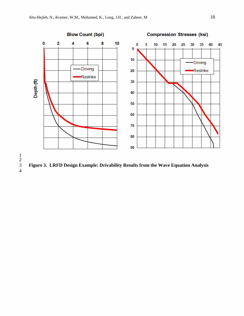
10 The drivability option is selected, where the output results for the driving and restrike conditions 11 are blow counts and driving stresses at various depths. Based on these results, Lmax for the 12 driving and restrike conditions can be identified. 13 14 LRFD Design Example: Determination of Lmax 15 16 The wave equation analysis program used to solve this example is the GRLWEAP program (5 17 and 6). 18 19 Input data: 20

• The estimated Rndr and Rnre resistance vs. depth curves for the wave equation analysis 21 shown in Figure 2b. 22

• Several types of hammers were evaluated in the drivability analysis. A D30-23 diesel 23 hammer was selected because it is a commonly available hammer. A hammer efficiency 24 of 80% is selected. 25

• The maximum tolerable driving stress, σdr-max, for steel is 0.9fy = 45 ksi, and the 26 maximum permissible penetration resistance is 10 bpi. 27

• The drivability resistance factor, φda, is 1. 28 29

Output results. The results of drivability option in terms of blow counts and compression 30 stresses at various depths for driving and restrike conditions are provided in Figure 3. Lmax is 31 obtained from Figure 3 at the depth where the limiting conditions for driving stresses (45 ksi) or 32 blow count (10 bpi) are met: 87 ft for driving conditions and 73 ft for restrike conditions. To 33 account for uncertainties in the design procedure suggested in this paper for estimation of Lmax, 34 conservative (smaller) Lmax of 80 ft for driving conditions and 70 ft for restrike conditions are 35 selected to solve the LRFD Design Example. 36 37 STRUCTURAL COMPRESSION RESISTANCE OF A PILE AT THE STRENGTH 38 LIMIT STATE 39 40 The governing LRFD design equation for this limit state is: 41 42

Qf ≤ φstr Pn (12) 43 44 Qfmax-structural is defined as the maximum factored axial compression load, Qf, that can be applied 45 to the top of a single pile based on the pile structural resistance, which can be computed based on 46


Eq. 12 as Qfmax-structural = φstr Pn . 1 2 LRFD Design Example: Determination of Qfmax-structural. 3 4 The axial compression structural resistance for H-pile is computed as Pn = Asfy , and Qfmax-structural 5 is determined as 0.6 x 50 x 15.5 = 465 kips. 6 7 DETERMINATION OF THE MAXIMUM FACTORED AXIAL COMPRESSION LOAD 8 (QFMAX) 9 10 Qfmax-geotechnical is defined as the maximum factored axial compression load a pile can support 11 based on meeting the geotechnical and drivability limit states (not structural). It can be 12 determined from the developed Qf vs. depth curve as the Qf at Lmax, so Qfmax-geotechnical meets both 13 the geotechnical and drivability limit states. 14 15 Qfmax can be determined as the smaller of Qfmax-structural and Qfmax-geotechnical. The structural limit 16 state controls Qfmax for piles seated on top of very hard rocks as discussed before. For piles 17 driven into soils and weak rocks, the geotechnical strength and drivability limit states control 18 Qfmax in most cases, but could be controlled by the structural limit state when static load test is 19 selected as will demonstrated in the solution of the LRFD Design Example. 20 21 All the strength limit states for compression resistance of a single pile (geotechnical, drivability, 22 and structural) can be addressed by keeping 23 24

Qf ≤ Qf max (13) 25 26 DEVELOPMENT AND APPLICATIONS OF DESIGN CHARTS 27 28 The information obtained from addressing all the strength limit states for compression resistance 29 of a single pile can be summarized in a design chart that include 30

• Curves of pile nominal bearing resistances at various depths up to Lmax 31 • A curve of pile factored loads (Qf ) vs. depth up to Qfmax. 32

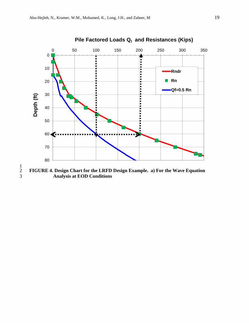
These charts can be used to develop Qfmax, and the pile length, L, and field nominal bearing 33 resistances required to support any Qf. The development and applications of the design charts are 34 demonstrated in this section by solving the LRFD design Example. Other applications of design 35 charts are also discussed later. 36 37 Note. GL (Lost nominal bearing resistance) due to local scour is 3.5 kips, evaluated as the total 38 of side resistances in the top 15 ft of the soil layer. 39 40 Wave Equation Analysis at EOD Conditions 41 42 The developed design chart in Figure 4a include Rnfield and Rndr vs. depth curves (from Figure 2b) 43 and Qf vs. depth curve obtained using Qf = 0.5Rnfield. At Lmax= 80 ft, the Qfmax-geotechnical is 44 obtained from the Qf vs. depth curve as 191 kips. This value is less than Qfmax-structural, so Qfmax = 45 191 kips. 46


1 As demonstrated in the design chart: 2

• The pile length to support Qf of 100 kips is estimated as 60 ft, obtained from the Qf vs. 3 depth curve at Qf= 100 kips. 4

• Use the Rndr vs. depth curve and pile length of 60 ft to determine the required Rndr as 5 203.5 kips. Alternately, the required Rndr can be computed using Eq. 7 as 100/0.5 + 3.5 = 6 203.5 kips. 7

8 Wave Equation Analysis at BOR Conditions 9 10 The developed design chart in Figure 4b include Rnfield, Rndr, Rnre vs. depth curves (from Figure 11 2b) and Qf vs. depth curve obtained using Qf = 0.5Rnfield. Lmax = 70 ft is obtained from the 12 drivability analysis for restrike conditions. At this Lmax, the Qfmax-geotechnical is obtained from the 13 Qf vs. depth curve as 209 kips. This value is less than Qfmax-structural, so Qfmax = 209 kips. 14 15 As demonstrated in the design chart: 16

• The pile length to support Qf of 100 kips is estimated as 51 ft. 17 • Use the Rnre vs. depth curve and pile length of 51 ft to determine the required Rnre as 203.5 18

kips. Alternately, the required Rnre may be computed using Eq. 8 as 100/0.5 + 3.5 = 203.5 19 kips. 20

• Use the Rndr vs. depth curve at a depth of 51 ft to determine the required Rndr as 139 kips. 21 Initially, drive the test pile should to this resistance at EOD and later restrike it to verify 22 the higher restrike resistance (Rnre) of 203.5 kips. 23 24

Axial Compression Static Load Test 25 26 The Qf vs. depth curve for the load test presented in Figure 5 is developed using Qf = 0.8Rnfield. 27 Since restrike is not needed with static load tests, all benefits of setup up to a depth of Lmax= 80 ft 28 can be assumed in the design. At Lmax= 80 ft, the Qfmax-geotechnical is obtained from the Qf vs. depth 29 curve as 479 kips, which is larger than Qfmax-structural = 465 kips, so Qfmax = 465 kips, controlled by 30 the pile structural resistance. As demonstrated in Figure 5, the pile length to support Qf of 100 31 kips is estimated as 41 ft. The required Rnre that should be verified with the static load test is 32 computed using Eq. 8 as 100/0.8+ 3.5 = 128 kips. Initially, drive the test pile until two 33 requirements are met: a depth of 41 ft and a required Rndr at EOD of 85 kips, the later obtained 34 based on the EOD wave equation analysis (Figure 2b) as discussed before. Later, verify with the 35 static load test that required resistance of 128 kips (or more) is obtained. Finally, it is 36 recommended that the test pile for a static load test is driven to a depth larger than the depth 37 developed in the design. 38 39 Discussion 40 41 Figure 5 presents the Qf vs. depth design curves up to Qfmax and Lmax for all investigated field 42 analysis methods. Results of all investigated field analysis methods are summarized in Table 1. 43 As the Qf that can be supported at any depth and Qfmax increases, respectively, the pile length and 44 number of piles in a pile group will decrease. 45 46


Based on the results summarized in Figure 5 and Table 1, the advantages of considering setup in 1 the design and using static load tests are: 2

• By comparing the wave equation analysis at EOD and BOR conditions, the benefits of 3 verifying setup at BOR conditions can be recognized as either reducing pile length (by 9ft 4 from 60 to 51 ft) or number of piles (larger Qfmax at smaller Lmax for BOR conditions than 5 for EOD conditions). 6

• With the use of static load test, the estimated pile length will be the smallest (41 ft) and 7 Qfmax would be the largest (465 kips), which is more than twice the Qfmax estimated for 8 the wave equation analysis at BOR conditions (209 kips). This means that number of 9 piles in a group of piles with the static load test could be less than half of those obtained 10 with the wave equation analysis at BOR conditions, assuming pile compression 11 geotechnical resistance would control the pile depths in the design. Reasons for better 12 performance of static load tests are: 13 • Static load test has the highest resistance factor (0.8) because it is the most accurate 14

field analysis method. 15 • Static load tests allow reaping all the benefits of large site-specific setup without the 16

need for restrike. This is why Lmax of 80 ft is considered to estimate Qfmax for the 17 static load test. However, smaller Lmax of 70 ft is considered for the wave equation 18 analysis at BOR conditions because restrike is needed in that case to verify the 19 required bearing resistance. 20 21

IMPROVE THE LRFD DESIGN PROCESS FOR DRIVEN PILES 22 23 As previously demonstrated, the design charts provide a simple and flexible approach for the 24 foundation designers to obtain the data needed for the construction plans, such as pile length, L, 25 and required field nominal bearing resistance for any applied Qf. Hence, design charts can easily 26 handle continuous changes in the applied Qf loads which is common in the design. 27 28 In addition, design charts (as in Figure 4) and design curves (as in Figure 5) can be used to 29 optimize, speed, and finalize the LRFD design for a pile group by: 30

• Addressing drivability of pile lengths determined in the design from addressing all 31 applicable LRFD limit states (not only strength limit state) by keeping these lengths less 32 than Lmax as previously discussed. 33

• Addressing all strength limit states for compression resistance of a single pile by keeping 34 Qf ≤ Qfmax 35

• Comparing various candidate pile types with a certain field analysis method and select 36 the most appropriate pile type (develop a figure like Figure 5 for the candidate pile 37 types). 38

• Comparing the candidate field analysis methods (e.g., static load test, wave equation, 39 dynamic formula) with a certain pile type (like in Figure 5) and select the most 40 appropriate field analysis method It is recommended that designers always consider a 41 static load test as a candidate field analysis method in the preliminary design. In the final 42 design, the most appropriate field analysis method should be selected by evaluating 43 various candidate analysis methods and comparing them based on savings in construction 44 costs and construction time. 45


• Evaluating various layouts for a pile group and select the most cost-effective layout 1 (number, location, and depth of piles). 2

3 Abu-Hejleh et al. (3) provided detailed recommendations to improve the LRFD design process 4 for driven piles. 5 6 IMPLEMENTATION 7 8 This paper will be of immediate interest to State DOT geotechnical and structural engineers 9 involved in the LRFD design of driven piles and the development of LRFD design specifications 10 for driven piles. It will help those engineers address many problems facing them with 11 implementation of AASHTO LRFD design specifications for driven piles. It will also help them 12 to develop more accurate and economical LRFD design methods for driven piles than commonly 13 used in practice. 14 15 ACKNOWLEDGEMENT 16 17 The authors would like to acknowledge Dr. Scott Anderson from the FHWA for his technical 18 reviews and continuous support of this work. 19 20 REFERENCES 21 1. Abu-Hejleh, N., DiMaggio, J.A., Kramer, W.M., Anderson, S., and Nichols, S. (2010). 22

“Implementation of LRFD Geotechnical Design for Bridge Foundations.” FHWA-NHI-10-23 039, National Highway Institute, Federal Highway Administration, Washington, D.C. 24 https://www.fhwa.dot.gov/resourcecenter/teams/geotech/publications.cfm 25

2. AASHTO (American Association of State Highway and Transportation Officials) (2014). 26 “AASHTO LRFD Bridge Design Specifications, 7th Edition,” Washington, D.C. 27

3. Abu-Hejleh, N., Kramer, W.M., Mohamed, K., Long, J.H., and Zaheer, M (2013). 28 “Implementation of AASHTO LRFD Design Specifications for Driven Piles.” FHWA-RC 29 13-01, Federal Highway Administration, Washington, D.C. 30 https://www.fhwa.dot.gov/resourcecenter/teams/geotech/publications.cfm 31

4. Abu-Hejleh, N., Kramer, W.M., Mohamed, K., Long, J.H., and Zaheer, M. (2015). 32 “Implementation of LRFD Geotechnical Strength Limit State for Compression Resistance of 33 Single Driven Pile.” TRB 2015 Annual Meeting Compendium of Papers, Transportation 34 Research Board, Washington, DC. 35

5. Hannigan, P.J., Rausche, F., Likins, G.E., Robinson, B.R., and Becker, M.L. (2016). 36 “Geotechnical Engineering Circular No. 12– Design and Construction of Driven Pile 37 Foundations.” FHWA-NHI-16-009, National Highway Institute, Federal Highway 38 Administration, Washington, D.C. 39

6. Hannigan, P.J., Goble, G.G., Likens, G.E., and Rausche, F. (2006). “Design and Construction 40 of Driven Pile Foundations.” FHWA-NHI-05-042, National Highway Institute, Federal 41 Highway Administration, Washington, D.C. 42

43 44

45 46

https://www.fhwa.dot.gov/resourcecenter/teams/geotech/publications.cfm

https://www.fhwa.dot.gov/resourcecenter/teams/geotech/publications.cfm


1 2


1 2 3

4 5

FIGURE 1. Details of the LRFD Design Example 6 7

Cohesionless mixed soil 31 ft Friction angle = 31o Saturated unit weight =110 pcf

12x53 H-pile: fy = 50 ksi As = 15.5 in2 Box area = 1 ft2 Perimeter = 4 ft φstr = 0.6

Hard clay: Undrained shear strength = 8 ksf Saturated unit weight= 125 pcf, Setup= 50%

Top 15 ft subjected to local scour

Ground water level (GWL) at ground level

With various field analysis methods determine: Lmax and Qfmax Pile Length, L Required nominal bearing resistance

Qf = 100 kips


1 FIGURE 2. LRFD Design Example. a) Pile Bearing Resistances from the β-Method 2 3

4 5 6

0

10

20

30

40

50

60

70

80

0 100 200 300 400 500 600 700

Dep

th (f

t) Pile Bearing Resistances at Various Stages (kips)

Rnre

Rndr

Rn= Rnsta


1 FIGURE 2 (continued). b) Pile Bearing Resistances for Wave Equation Analysis at EOD 2 and BOR Conditions 3 4 5

6

0

10

20

30

40

50

60

70

80

90

0 100 200 300 400 500

Dep

th (f

t) Pile Bearing Resistances at Various Stages (kips)

Rndr

Rnre

Rn = Rnfield, BOR Conditions

Rn = Rnfield, EOD Conditions


1 2 Figure 3. LRFD Design Example: Drivability Results from the Wave Equation Analysis 3 4


1 FIGURE 4. Design Chart for the LRFD Design Example. a) For the Wave Equation 2

Analysis at EOD Conditions 3

0

10

20

30

40

50

60

70

80

0 50 100 150 200 250 300 350

Dep

th (f

t) Pile Factored Loads Qf and Resistances (Kips)

Rndr

Rn

Qf=0.5 Rn


1 2 FIGURE 4 (continued). b) For the Wave Equation Analysis at BOR Conditions 3 4 5 6 7 8

0

10

20

30

40

50

60

70

0 50 100 150 200 250 300 350

Dep

th (f

t) Piles Resistances and Factored Load, Qf (Kips)

Rnre

Rn

Rndr

Qf=0.5 Rn


1 2

3 4 FIGURE 5. Design Curves for all Investigated Field Analysis Methods 5 6 7 8

TABLE 1. Results of the Field Analysis Methods 9 Method Results for Qf = 100 kips

Lmax (ft)

Qfmax (kips)

Pile Length or Depth

(ft)

Required Nominal Bearing Resistance

(kips) Rndr Rnre

Wave Equation (EOD) 60 203.5 N/A 80 191

Wave Equation (BOR) 51 139 203.5 70 209

Static Load Test 41 85* 128** 80 465 *Assuming resistance verification with wave equation analysis. See body the paper for more. 10 ** Verified by the static load test 11 12

0

10

20

30

40

50

60

70

80

0 50 100 150 200 250 300 350 400 450 500

Dep

th (f

t)

Top Factored Axial Compression Loads Qf

Static Load Test

Wave Equation Analysis at BOR

Wave Equation Analysis at EOD

Structural Strength Limit

rational gudiance to determine the maximum factored …docs.trb.org/prp/17-05334.pdf · rational...

Documents