rationing in the market for new housing
TRANSCRIPT

Rationing in the Market for New Housing
David Sunding
College of Natural Resources
University of California–Berkeley
Aaron M. Swoboda
Graduate School of Public and International Affairs
University of Pittsburgh
Abstract
The paper investigates the possibility that regulation influences the price of housing by di-
rectly limiting the quantity of new housing produced. This possibility is in contrast to the
usual treatment of regulation in the housing literature, which is to assume regulation influ-
ences the housing market by increasing the cost of development, including land assembly.
The paper presents strong evidence that new housing is rationed in Southern California by
examining sales of over 18,000 newly-constructed homes in three inland counties. The es-
timated shadow price of new housing is in excess of $85,000 per unit in many areas, and is
shown to be significantly associated with measures of the intensity of local housing regu-
lation. These results suggest that the possibility of regulatory rationing should play a more
central role in models of housing and the urban economy.
1 Introduction
An extensive literature attempts to measure the impacts of regulation in the housing
market. 1 Most studies are predicated on the standard treatment of land as a factor
of housing production and assume that regulation affects the price of housing by
increasing the price of land and other costs of development. We investigate the
possibility that regulation directly limits the quantity of new housing produced in
an area by preventing developers from optimally subdividing land. Rationing of the
housing stock is a much stronger form of regulation than standard land use controls.
In fact, the possibility that housing is rationed causes some of the findings of the
standard urban economics model to fail.
In the neo-classical framework developed by Alonso [1], Mills [21, 22], Muth [23]
and Beckmann [2] taught to every graduate student in urban economics, land is
treated as a production factor for two competing goods, housing construction and
yard space. The equilibrium marginal value product of land for these competing
uses should be equal; consumers’ marginal valuation of lot size is equal to the eco-
nomic returns to land from additional housing construction. If this equality does not
hold, developers can increase their profits by reallocating land toward the higher
valued use. However, the returns to housing construction per unit of land will ex-
ceed consumers’ marginal valuation of land when subdivision is constrained and
1 For example, Dowall and Landis [6], Mark and Goldberg [16], Katz and Rosen [14],Pollakowski and Wachter [25], and Green [12] examine the effect of land use regulation onthe price of housing while Maser et al. [18], Knaap [15], Rose [27], and Shilling et al. [30]examine the effects of regulation on land prices.
1

there is a limited supply of developable land. New housing construction will earn
positive economic profits if regulation limits production in this way.
As suggested by Glaeser and Gyourko [10], this line of reasoning suggests a test for
the presence of rationing in the housing market. We construct a dataset of 18,697
newly constructed homes sold in the Inland Empire of Southern California between
1993 and 2003. Limiting attention to new homes greatly aids in the analysis since
the land was subdivided recently and avoids issues of housing vintage. We use a
Geographic Information System to avoid problems of over-aggregation and allow
for variation in the price of land, and construction costs. We use geographically
weighted regression techniques to estimate the return to land for additional lot size
while the returns to land for additional construction are calculated by combining
location and quality specific construction cost data with the sales data.
Our analysis finds strong evidence of regulatory rationing: the return to land from
new construction is significantly greater than the return from increased lot size in
much of the study area. The median estimated shadow value of housing is almost
$50,000, with nearly one quarter of our estimates greater than $85,000 per house
in our study area. We also show that areas with regulatory regimes characterized
as anti-growth by Glickfeld and Levine [11] and Quigley et al. [26] are associated
with higher shadow prices of housing.
The fact that housing is rationed has significant implications for the study of the
urban economy. First, regulatory rationing creates economic rents that will not be
2

captured by the marginal price of land. Thus, the price of land will underestimate
the welfare costs of regulations that further limit new housing construction. Second,
regulations that directly limit the quantity of new housing may reduce densities.
Rationing prompts developers to produce housing with larger lot sizes than they
otherwise would. In fact, low density development and other common indicators
of urban sprawl may themselves be a consequence of regulatory rationing. Third,
rationing implies that the price of housing is determined through an auction-like
process rather than by the cost of factors of production. As a result, taxes on land
and other factors of production will be less effective than with optimal subdivision,
and rather act as wealth transfers. This idea may explain the findings of Mayer and
Somerville [19], who show that fees and taxes on development had little effect on
the level of new construction in their panel data of 44 metropolitan areas between
1985 and 1996.
The remainder of the paper is laid out as follows. The next section provides a dis-
cussion of the housing and land markets with and without regulatory rationing and
develops the conceptual framework for the paper. Section 3 describes the study re-
gion and data used in the analysis. Section 4 presents the econometric estimates
of consumers’ valuation of additional lot size. Section 5 estimates of the value of
land for new housing construction across our study area. Section 6 presents a test
of the null hypothesis of no regulatory rationing. Section 7 estimates the shadow
price of housing across our study area and shows the robustness of our results to
differing model assumptions. Section 8 analyzes the relationship between our esti-
3
mated shadow prices of new housing and measures of land use regulation across the
region. We conclude with a brief summary of the paper and a discussion of future
research in the area.
2 Regulation and the Housing Market
Imagine a profit maximizing firm choosing the number of houses to build and the
amount of land associated with each house in a particular neighborhood. Let H be
the total number of houses produced, L be the quantity of land used per house, and
P represent the price of a housing bundle, including the house and lot. The function
P(·) relates the price of the home to the amount of land associated each house
and the total number of houses built in the neighborhood, although we assume
producers only directly affect the price through changes in lot sizes. Let the land
market be defined by a fixed amount of developable land, N. The producer’s profit
maximization problem is,
maxL,H,µ π = P(L,α)H −K(H)+µ(N −LH), (1)
where µ is the price of land. Optimal production occurs where P−KH −µL = 0, and
PLH − µH = 0. The equilibrium house price is equal to the marginal construction
and development costs plus the equilibrium price of the land it is built upon. Fur-
ther, the price of land, denoted by µ, is equal to consumers’ marginal willingness
to pay for lot space. Combining these equations yields the condition for optimal
4
subdivision, namely,
P−KH
L−PL = 0. (2)
In words, this condition requires that the value of land used to produce additional
housing is equal to consumers’ marginal valuation of yard space. 2 In effect, con-
sumers purchase yard space by bidding land away from new housing construction
until their marginal valuation of land is equal to the returns to land from housing
construction. If this equality did not hold, a profit maximizing housing developer
could increase its profits by devoting more land to the higher valued use.
The equilibrium results of Brueckner [3] can be used to show this subdivision
condition is a direct result of extending the urban economics literature developed
by Alonso [1], Mills [21, 22], Muth [23] and Beckmann [2]. This neo-classical
literature assumes that land is the scarce resource and accrues Ricardian rents.
Somerville [31] examines the contribution of land and structure to builder profits
using a model of land scarcity and a micro-dataset of homebuilder land and struc-
ture expenditures. He finds a smaller than expected markup on land expenditures
than predicted under a system of land scarcity. The coefficient on land expenditures
is not significantly different from one for a majority of the Metropolitan Statisti-
cal Areas in his study. Rosenthal [29] concludes the implicit market for residential
buildings is efficient in Vancouver, British Columbia from 1979–1989 since devia-
tions between the price of new buildings and their construction costs are dissipated
2 In the terminology of Glaeser and Gyourko [10], these are the extensive and intensivemargin values of land.
5
more quickly than the time required for new construction. He concludes that any
inefficiencies in the housing market must lie in the market for land.
We now examine the possibility that regulation places direct limits on the amount of
new housing produced. Regulatory rationing and binding density constraints create
economic rents that cannot be captured in the land market. Assume that regulation
constrains the maximum number of houses produced in a neighborhood to be H
and λ is the shadow price of housing. Equation (1) is now replaced by
maxL,H,µ,λ π = P(L,α)H −K(H)+µ(N −LH)+λ(H −H). (3)
The equilibrium relationships between the variables of interest are shown in equa-
tion (4). Consumers’ willingness to pay for more land and the value of land for
new housing construction are no longer equal. Rather, because regulation limits the
number of houses produced, the returns to land used to construct additional hous-
ing, P−KHL , are greater than consumers’ valuation of land for additional yard space,
PL. 3
P−KH
L−PL =
λ
L> 0 (4)
The possibility of rationing is of interest because the impacts of policy interven-
tions in a rationed market will differ from the impacts in a standard equilibrium.
For instance, equation (4) shows taxes on housing production will have no effect
3 Producer market power will cause P−KHL > PL, however there seems to be little reason to
suspect significant producer market power in the absence of regulations that limit entry andproduction.
6

on output as long as the tax is less than λ. Land restrictions or taxes will cause noth-
ing more than an increase in housing density, if allowed by the regulatory regime.
However, policies that further limit housing production will have marginal costs
equal to the existing shadow price of housing, much larger than that predicted un-
der the standard model.
The conclusions that can be drawn from comparing the values of land for yard
space and new construction are important but limited. In particular, this test is not
an indication of the presence or absence of regulation’s impacts on the price of
housing. In a nation-wide study Glaeser and Gyourko [10] examine the relation-
ship between regulation and housing affordability using a statistical test similar to
equation (4). However, many common types of land use regulation, such as Urban
Growth Boundaries, location restrictions, and land taxes, may have large impacts
on the equilibrium house price, but will not be detected under a test such as this
one if their primary impacts are increases in the price of land. The value of land
for new housing construction will still equal the value of land for additional yard
space as long as these policies allow producers to optimally subdivide. Conversely,
governments may institute a rationing regime in the housing market and create a
positive shadow price in the market, yet only have a minimal impact on the price
of housing. Nonetheless, by making the supply curve more inelastic, direct con-
trols on the quantity of new housing can create a precondition for significant price
appreciation in the face of a demand shock.
7

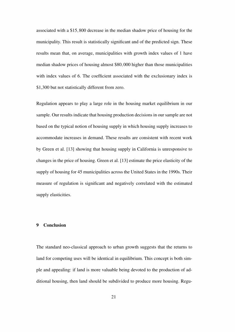
Figure 1. Overview of the Study Area
� ��
�
�
����������
�������
� ���
���������
��������������
�� ����
���������
�����
������
�����
���� ��
�����
���� ��
����
�����
�
���������
����������������� ���������������������
����������������
����������������
�������������
� �� �����
��������������� ���
������������
������� ����������������
3 Southern California Housing Data
Our empirical analysis is performed using housing market data from 18,697 newly
built home sales transactions between 1993 and 2002 in Southern California, in-
cluding parts of Los Angeles, San Bernardino and Riverside Counties (see Figure
1). This region is characterized by high rates of recent growth and represents a
substantial portion of Los Angeles’ exurban growth.
Each observation consists of basic sales characteristics and the physical attributes
of the home, including its exact latitude and longitude allowing for the use of Ge-
ographic Information Systems. A “median house” for the entire region would have
8

four bedrooms, two-and-a-half bathrooms, 2,144 square feet of living space, a lot
size of 7,405 square feet, and sell for approximately $275,000 in year 2003 dollars.
The data are commercially available through DataQuick. com, a company that ag-
gregates and distributes real estate data. Table 1 summarizes the relevant variables
within the study region.
All analysis is in year 2003 US Dollars; sales prices are converted using the Con-
ventional Mortgage Home Price Index (CMHPI) by Freddie Mac. 4 This index uses
repeat home sales to establish a price index for Metropolitan Statistical Areas (de-
fined by the Office of Management and Budget) over time in order to compare home
prices across time. The indices for Los Angeles and San Bernardino/Riverside
are used for this analysis. The mean (median) adjusted sale price is $301,000
($275,000) with a standard deviation of $118,000.
The median lot size for the study region is 7,405 ft2, with a mean of roughly 8,200
ft2. 5 The mean (median) living space across the study region is just over 2,200
(2,144) square feet, with a standard deviation of approximately 700. The mean
(median) number of bedrooms is 3.8 (4) with a standard deviation of .9. The mean
(median) number of bathrooms is 2.6 (2.5) with a standard deviation of .6.
4 The CMHPI data are published quarterly and are available athttp://www.freddiemac.com/finance/cmhpi/.5 The data are censored to include only observations with lots less than an acre (this re-moves fewer than .9% of the observations).
9
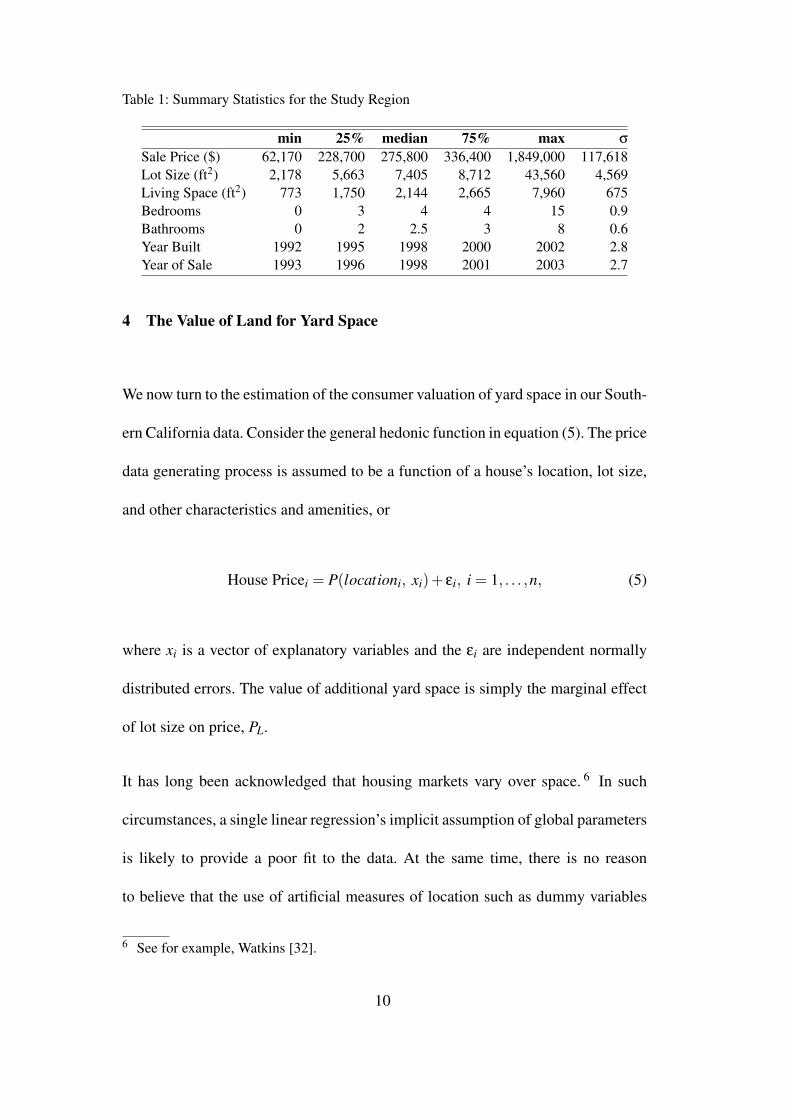
Table 1: Summary Statistics for the Study Region
min 25% median 75% max σ
Sale Price ($) 62,170 228,700 275,800 336,400 1,849,000 117,618Lot Size (ft2) 2,178 5,663 7,405 8,712 43,560 4,569Living Space (ft2) 773 1,750 2,144 2,665 7,960 675Bedrooms 0 3 4 4 15 0.9Bathrooms 0 2 2.5 3 8 0.6Year Built 1992 1995 1998 2000 2002 2.8Year of Sale 1993 1996 1998 2001 2003 2.7
4 The Value of Land for Yard Space
We now turn to the estimation of the consumer valuation of yard space in our South-
ern California data. Consider the general hedonic function in equation (5). The price
data generating process is assumed to be a function of a house’s location, lot size,
and other characteristics and amenities, or
House Pricei = P(locationi, xi)+ εi, i = 1, . . . ,n, (5)
where xi is a vector of explanatory variables and the εi are independent normally
distributed errors. The value of additional yard space is simply the marginal effect
of lot size on price, PL.
It has long been acknowledged that housing markets vary over space. 6 In such
circumstances, a single linear regression’s implicit assumption of global parameters
is likely to provide a poor fit to the data. At the same time, there is no reason
to believe that the use of artificial measures of location such as dummy variables
6 See for example, Watkins [32].
10
for zip code, census tract, or Federal Information Processing Standard (FIPS) will
capture the appropriate spatial variation of PL and other factors.
We take advantage of our geo-referenced data and use a geographically weighted
regression (GWR) model to estimate the marginal value of yard space across our
study region. 7 This technique employs weighted least squares regression to es-
timate location-specific regression parameters using a weights matrix, W , where
element wi j is a function of the distance between observation i and j. GWR al-
lows continuous variation in the regression parameters irrespective of artificially
imposed boundaries and represents a natural extension to “spatial expansion” meth-
ods in which space is parameterized using polynomials. 8
We allow the regression coefficients to vary over space by estimating βi according
to equation (6) for each location within the dataset, i = 1, . . . ,n.
βi = (X ′WiX)−1X ′WiP, ∀ i = 1, . . . , n (6)
X is an n×k matrix of explanatory variables, Wi is an n×n weighting matrix, where
W [i, j] is 1/k if observation j is one of the k geographically nearest neighbors to
observation i, and 0 otherwise, and P is the vector of observed house prices. For
each observation, we perform a weighted linear regression and assign the resulting
βi vector to the location of observation i. In this manner, the regression coefficients
7 Examples of this regression technique are Cleveland and Devlin [5], McMillen [20],Fotheringham et al. [8], Pavlov [24] and is summarized in Fotheringham et al. [9].8 See, for example, Casetti [4].
11
are allowed to vary across space as the data suggest. 9
Table 2 shows how the predictive power of GWR compares to other regression
models for our data sample. In particular, we compare the root mean square cross-
validation error (RMSCVE) generated from a single linear regression (no spatial
variation in any parameters), linear regression with municipality dummies (limited
spatial variation of intercept), linear regression with municipality interactions (pa-
rameterized spatial variation of all regressors by FIPS code), and geographically
weighted regression with varying k parameters (non-parameterized spatial variabil-
ity in all regressors). We use drop-one cross-validation to calculate the RMSCVE
for the GWR models as in equation (7), which compares the true value yi to the
estimated value when observation i is omitted from the calibration, y6=i. Dropping
observation i prevents the observation from having undue influence in the estima-
tion process as k decreases.
RMSCV E =
[n
∑i=1
(yi − y6=i)2
n
].5
(7)
The RMSCVE is smallest ($35,329) when k = 50, approximately half the size of
the $69,468 associated with a single global linear regression, and nearly 20 percent
lower than the value associated with municipality interaction variables. Comparing
the RMSCVE across models of varying k allows us to choose the k value that bal-
ances the tradeoff between biased estimates from not incorporating enough spatial
9 Note: when k = n the model is equal to Ordinary Least Squares.
12

Table 2: Root Mean Square Cross Validation Error (RMSCVE) for Alternative Models
Model RMSCVESingle linear regression $69,468Linear regression with municipality dummies $49,496Linear regression with municipality interactions $43,163Geographically weighted regression, k= 500 $39,641Geographically weighted regression, k= 300 $38,329Geographically weighted regression, k= 200 $37,228Geographically weighted regression, k= 100 $35,723Geographically weighted regression, k= 75 $35,458Geographically weighted regression, k= 50 $35,329Geographically weighted regression, k= 25 $38,146Note: The mean distance to the kth nearest observation is 3.0,2.0, 1.4, .79, .63, .43, and .24 miles.
variation, k too large, and sample error from k too small. For the remainder of the
paper, we use the estimates associated with k = 50, although the results are robust
to other modeling choices. Table 3 displays the mean and standard deviation of
the parameter estimates from three representative geographically weighted regres-
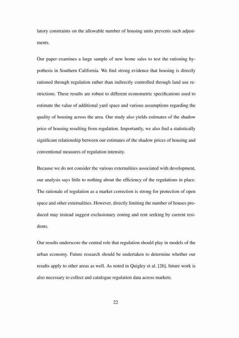
sions. Figure 2 displays the spatial distribution of the estimated marginal effect of
lot size on the price of housing across our study area. The estimates are also plotted
in Figure 3.
Table 3: Mean and St. Dev. of Geographically Weighted Regression Coefficients
k = 50 k = 100 k = 300mean σ mean σ mean σ
Lot Size ( f t2) 2.1 4.5 2.4 3.2 2.7 2.7Living Space ( f t2) 79 41 82 37 88 39Bathrooms 2,700 29,000 3,600 22,000 5,900 17,000Bedrooms -1,000 15,000 -2,200 12,000 -5,000 8,400Time 170 8,500 -24 6,100 -290 4,600(Intercept) 100,000 90,000 91,000 68,000 79,000 51,000
13
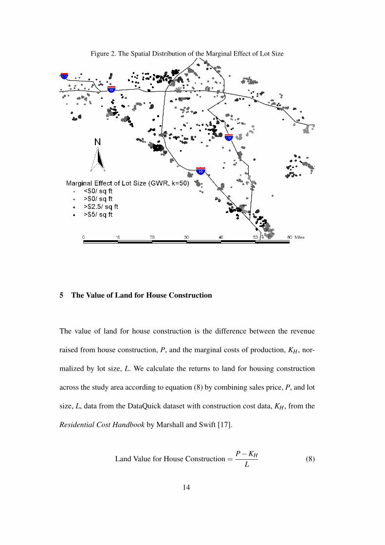
Figure 2. The Spatial Distribution of the Marginal Effect of Lot Size
5 The Value of Land for House Construction
The value of land for house construction is the difference between the revenue
raised from house construction, P, and the marginal costs of production, KH , nor-
malized by lot size, L. We calculate the returns to land for housing construction
across the study area according to equation (8) by combining sales price, P, and lot
size, L, data from the DataQuick dataset with construction cost data, KH , from the
Residential Cost Handbook by Marshall and Swift [17].
Land Value for House Construction =P−KH
L(8)
14

The Residential Cost Handbook provides cost data as a function of the county and
city, construction materials used, and overall quality level. We make the simplify-
ing assumption that all houses are of average quality. 10 11 We also include other
housing production costs, including site preparation, design, regulatory fees, and
marketing costs. We use an estimate of $35 per square foot of living space for
average quality homes, which is consistent with other work done in the area by
Economic and Planning Systems [7]. Under these assumptions the mean structural
costs are roughly $100 per square foot of living space with a standard deviation of
$4.30. Our estimates of the value of land for new housing construction have a mean
(median) of $10.70 ($8.10) per square foot, with a standard deviation of $9.8. The
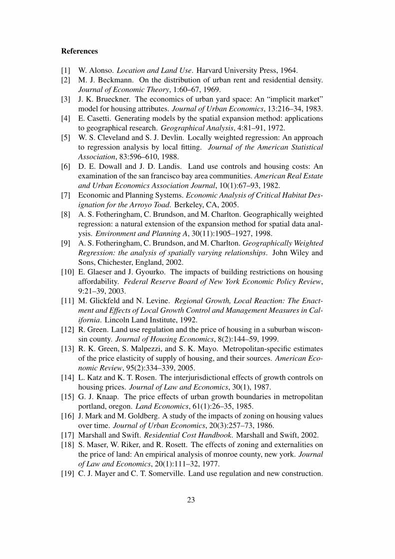
estimates are also plotted in Figure 3.
6 The Value of Land for New Construction vs. Yard Space
Under the standard model, the value of land for housing production minus con-
sumers’ valuation of additional yard space should be equal to zero. In our data,
the mean (median) difference is $8.58 ($6.37) per square foot of land, with a stan-
10 Marshall & Swift describe “average quality” homes as the most frequently encounteredresidence type. They are often mass produced and exceed the minimum construction re-quirements of lending institutions, mortgage insuring agencies and building codes. Work-manship is acceptable, but does not reflect custom craftsmanship. Cabinets, doors, hard-ware and plumbing are usually stock items. Architectural design includes ample fenestra-tion and some ornamentation. Carpet, hardwood, vinyl composition tile or sheet vinyl floorcover is used. Interior walls are taped and painted drywall with some inexpensive wallpa-per or paneling. Kitchen and bath have enamel painted walls and ceilings. Countertops arelaminated plastic or ceramic tile. Adequate number of electrical outlets with some luminousfixtures in kitchen and bath areas. Eight average-quality plumbing fixtures.11 We relax the assumption of average quality housing construction in a later section.
15
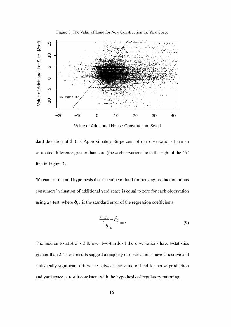
Figure 3. The Value of Land for New Construction vs. Yard Space
−20 −10 0 10 20 30 40
−10
−5
05
1015
Value of Additional House Construction, $/sqft
Val
ue o
f Add
ition
al L
ot S
ize,
$/s
qft
45 Degree Line
dard deviation of $10.5. Approximately 86 percent of our observations have an
estimated difference greater than zero (these observations lie to the right of the 45◦
line in Figure 3).
We can test the null hypothesis that the value of land for housing production minus
consumers’ valuation of additional yard space is equal to zero for each observation
using a t-test, where σPL is the standard error of the regression coefficients.
P−KHL − PL
σPL
= t (9)
The median t-statistic is 3.8; over two-thirds of the observations have t-statistics
greater than 2. These results suggest a majority of observations have a positive and
statistically significant difference between the value of land for house production
and yard space, a result consistent with the hypothesis of regulatory rationing.
16
7 The Shadow Price of Housing
We now give our results some context by estimating the shadow price of housing.
We use our estimates of the value of land for new house construction and addi-
tional yard space to calculate the shadow price of housing by rearranging equation
(4), λ = P−KH −PLL. The mean (median) estimated shadow price of new hous-
ing is approximately $63,000 ($49,000) with a standard deviation of approximately
$83,000. Almost one quarter of our observations have an estimated shadow price
greater than $85,000, and 68% of the estimates are statistically greater than zero.
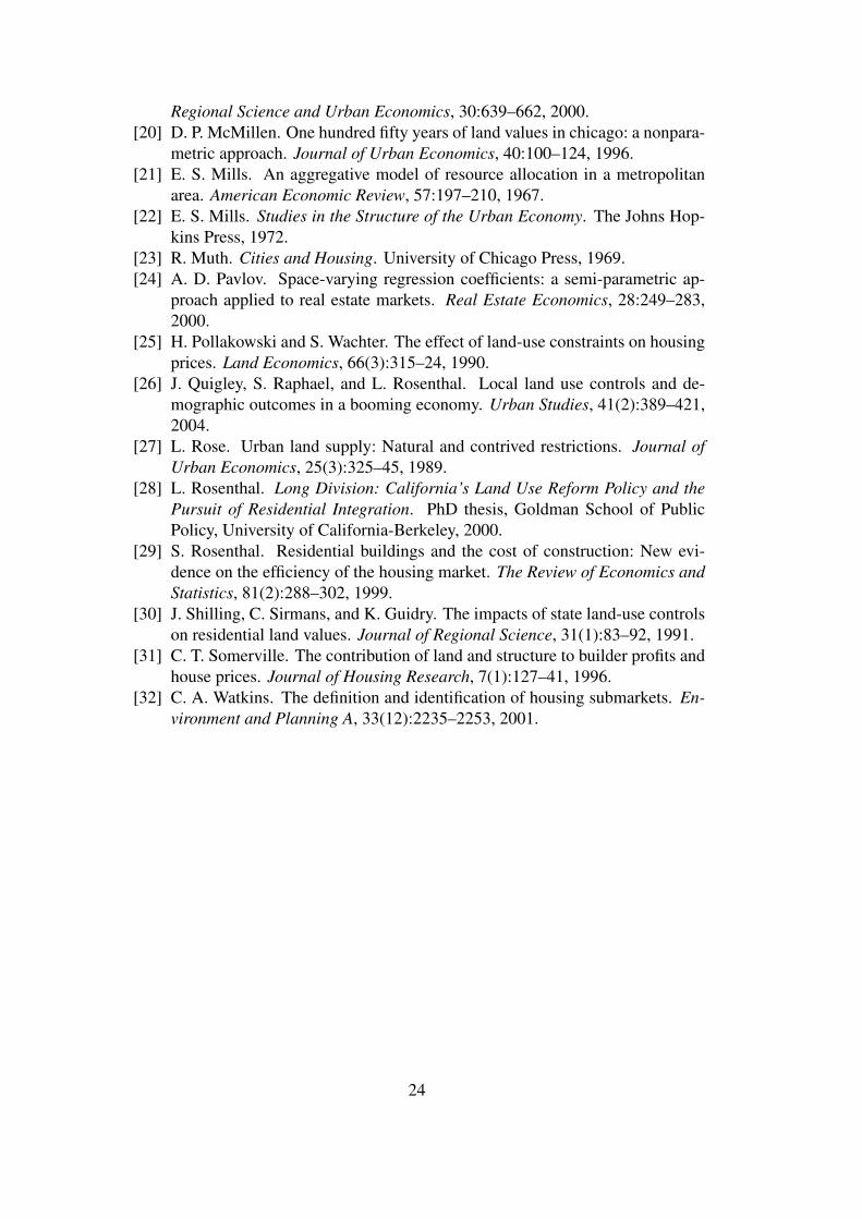
Figure 4 displays the spatial distribution of the median estimated shadow price of
new housing by municipality (as defined by Federal Information Processing Stan-
dards).
7.1 Result Robustness
Table 4 displays the robustness of our estimates under differing model assumptions.
The first three columns display the median estimated shadow price of housing by
municipality. The first column was calculated using the optimized geographically
weighted regression parameter, k = 50. The second column calculates the shadow
price of housing using the results from geographically weighted regression with
k = 300. The mean (median) estimates of the shadow price of housing are $57,000
($42,000), and 79% are statistically greater than zero. The third column estimates
the shadow rice of housing using a single Ordinary Least Squares regression. The
17
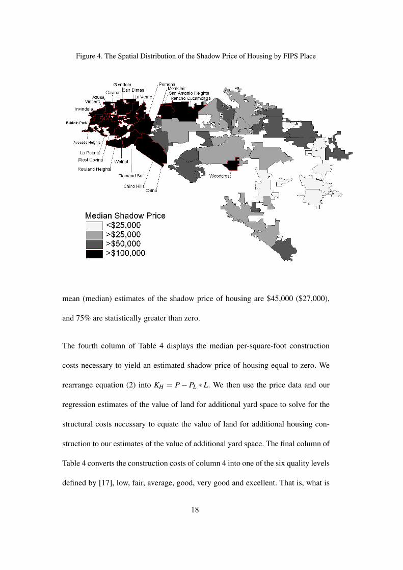
Figure 4. The Spatial Distribution of the Shadow Price of Housing by FIPS Place
mean (median) estimates of the shadow price of housing are $45,000 ($27,000),
and 75% are statistically greater than zero.
The fourth column of Table 4 displays the median per-square-foot construction
costs necessary to yield an estimated shadow price of housing equal to zero. We
rearrange equation (2) into KH = P−PL ∗ L. We then use the price data and our
regression estimates of the value of land for additional yard space to solve for the
structural costs necessary to equate the value of land for additional housing con-
struction to our estimates of the value of additional yard space. The final column of
Table 4 converts the construction costs of column 4 into one of the six quality levels
defined by [17], low, fair, average, good, very good and excellent. That is, what is
18
the median housing construction quality necessary to obtain the construction costs
in column 4? Of 61 total, in two municipalities the median construction quality is
fair, 13 municipalities remain average quality, 25 municipalities require good qual-
ity construction, 13 require very good quality, and 8 require excellent quality. We
find it implausible that in so many municipalities the median house qualities are
very good or above. 12
8 Regulation and the Shadow Price of Housing
We now explore the link between our estimates of the shadow price of housing and
local land use regulations. Glickfeld and Levine [11] conducted surveys of local
officials in the early 1990s to obtain land use regulation data. Quigley et al. [26]
and Rosenthal [28] use these data to construct regulatory measures by FIPS place.
In particular, a regulatory index was created for each municipality measuring the
extent to which the regulatory regime is “pro-growth” and “exclusionary”. Regu-
12 Marshall & Swift define very good quality as typical of those built-in high-quality tractsor developments and are frequently individually designed. Attention has been given to in-terior refinement and detail. Exteriors have good fenestration with custom ornamentationand trim. High-quality carpet, hardwood, sheet vinyl and ceramic tile. Vaulted or cathedralceilings in master bedrooms and entries. Spacious walk-in closets or wardrobes and largelinen closets.Marshall & Swift define excellent quality as individually designed and characterized by thehigh-quality of workmanship throughout, finishes and appointments and the considerableattention to detail. Excellent quality homes have high-quality carpet, hardwood (parquetor plank), terrazzo, and vinyl, ceramic, or quarry tile. Built-in bookshelves are commonlypresent as well as ample cabinetry, including cooking island, bar, desk, etc. Ceramic marbleor highest quality countertops. Ceilings include molding and coving with intricate detail,vaulted or cathedral ceilings found in family, dining room, bed rooms, etc. Raised panelhardwood doors. Spacious walk-in closets or wardrobes with many built-in features.
19

lations that determine the measure include restrictions on the number of building
permits issued, population growth restrictions, density restrictions, growth manage-
ment plans, and urban growth boundaries.
These data include regulation indices for 40 municipalities within our study region,
encompassing 14,694 of our 18,697 observations. The pro-growth index ranges
from 0 to 7 with higher values representing local government attitudes and reg-
ulations encouraging growth. The mean value for our data is 3.3 with a standard
deviation of 1.9. The exclusionary index ranges from 0 to 19, with larger values
representing local government attitudes and regulations preventing certain types of
growth. The mean value for our data is 9.7 with a standard deviation of 4.7. Table
5 displays the median shadow price of housing and the local regulatory indices by
FIPS place.
We perform a simple linear regression of median shadow price of housing on the
two regulatory indices. We use the median shadow price of housing since the mean
shadow price of housing is subject to skew from extreme values. We a priori as-
sume the pro-growth index to have a negative relationship with our estimate of the
shadow price of housing, as governments become more “pro-growth” it seems less
likely that housing is rationed in their municipality. We also predict that local gov-
ernments with “exclusionary” regulatory regimes are more likely to enact policies
that ration housing and increase the estimated shadow price of housing.
Table 6 displays the results of our regression. An increase in the pro-growth index is
20
associated with a $15,800 decrease in the median shadow price of housing for the
municipality. This result is statistically significant and of the predicted sign. These
results mean that, on average, municipalities with growth index values of 1 have
median shadow prices of housing almost $80,000 higher than those municipalities
with index values of 6. The coefficient associated with the exclusionary index is
$1,300 but not statistically different from zero.
Regulation appears to play a large role in the housing market equilibrium in our
sample. Our results indicate that housing production decisions in our sample are not
based on the typical notion of housing supply in which housing supply increases to
accommodate increases in demand. These results are consistent with recent work
by Green et al. [13] showing that housing supply in California is unresponsive to
changes in the price of housing. Green et al. [13] estimate the price elasticity of the
supply of housing for 45 municipalities across the United States in the 1990s. Their
measure of regulation is significant and negatively correlated with the estimated
supply elasticities.
9 Conclusion
The standard neo-classical approach to urban growth suggests that the returns to
land for competing uses will be identical in equilibrium. This concept is both sim-
ple and appealing: if land is more valuable being devoted to the production of ad-
ditional housing, then land should be subdivided to produce more housing. Regu-
21
latory constraints on the allowable number of housing units prevents such adjust-
ments.
Our paper examines a large sample of new home sales to test the rationing hy-
pothesis in Southern California. We find strong evidence that housing is directly
rationed through regulation rather than indirectly controlled through land use re-
strictions. These results are robust to different econometric specifications used to
estimate the value of additional yard space and various assumptions regarding the
quality of housing across the area. Our study also yields estimates of the shadow
price of housing resulting from regulation. Importantly, we also find a statistically
significant relationship between our estimates of the shadow prices of housing and
conventional measures of regulation intensity.
Because we do not consider the various externalities associated with development,
our analysis says little to nothing about the efficiency of the regulations in place.
The rationale of regulation as a market correction is strong for protection of open
space and other externalities. However, directly limiting the number of houses pro-
duced may instead suggest exclusionary zoning and rent seeking by current resi-
dents.
Our results underscore the central role that regulation should play in models of the
urban economy. Future research should be undertaken to determine whether our
results apply to other areas as well. As noted in Quigley et al. [26], future work is
also necessary to collect and catalogue regulation data across markets.
22
References
[1] W. Alonso. Location and Land Use. Harvard University Press, 1964.[2] M. J. Beckmann. On the distribution of urban rent and residential density.
Journal of Economic Theory, 1:60–67, 1969.[3] J. K. Brueckner. The economics of urban yard space: An “implicit market”
model for housing attributes. Journal of Urban Economics, 13:216–34, 1983.[4] E. Casetti. Generating models by the spatial expansion method: applications
to geographical research. Geographical Analysis, 4:81–91, 1972.[5] W. S. Cleveland and S. J. Devlin. Locally weighted regression: An approach
to regression analysis by local fitting. Journal of the American StatisticalAssociation, 83:596–610, 1988.
[6] D. E. Dowall and J. D. Landis. Land use controls and housing costs: Anexamination of the san francisco bay area communities. American Real Estateand Urban Economics Association Journal, 10(1):67–93, 1982.
[7] Economic and Planning Systems. Economic Analysis of Critical Habitat Des-ignation for the Arroyo Toad. Berkeley, CA, 2005.
[8] A. S. Fotheringham, C. Brundson, and M. Charlton. Geographically weightedregression: a natural extension of the expansion method for spatial data anal-ysis. Environment and Planning A, 30(11):1905–1927, 1998.
[9] A. S. Fotheringham, C. Brundson, and M. Charlton. Geographically WeightedRegression: the analysis of spatially varying relationships. John Wiley andSons, Chichester, England, 2002.
[10] E. Glaeser and J. Gyourko. The impacts of building restrictions on housingaffordability. Federal Reserve Board of New York Economic Policy Review,9:21–39, 2003.
[11] M. Glickfeld and N. Levine. Regional Growth, Local Reaction: The Enact-ment and Effects of Local Growth Control and Management Measures in Cal-ifornia. Lincoln Land Institute, 1992.
[12] R. Green. Land use regulation and the price of housing in a suburban wiscon-sin county. Journal of Housing Economics, 8(2):144–59, 1999.
[13] R. K. Green, S. Malpezzi, and S. K. Mayo. Metropolitan-specific estimatesof the price elasticity of supply of housing, and their sources. American Eco-nomic Review, 95(2):334–339, 2005.
[14] L. Katz and K. T. Rosen. The interjurisdictional effects of growth controls onhousing prices. Journal of Law and Economics, 30(1), 1987.
[15] G. J. Knaap. The price effects of urban growth boundaries in metropolitanportland, oregon. Land Economics, 61(1):26–35, 1985.
[16] J. Mark and M. Goldberg. A study of the impacts of zoning on housing valuesover time. Journal of Urban Economics, 20(3):257–73, 1986.
[17] Marshall and Swift. Residential Cost Handbook. Marshall and Swift, 2002.[18] S. Maser, W. Riker, and R. Rosett. The effects of zoning and externalities on
the price of land: An empirical analysis of monroe county, new york. Journalof Law and Economics, 20(1):111–32, 1977.
[19] C. J. Mayer and C. T. Somerville. Land use regulation and new construction.
23
Regional Science and Urban Economics, 30:639–662, 2000.[20] D. P. McMillen. One hundred fifty years of land values in chicago: a nonpara-
metric approach. Journal of Urban Economics, 40:100–124, 1996.[21] E. S. Mills. An aggregative model of resource allocation in a metropolitan
area. American Economic Review, 57:197–210, 1967.[22] E. S. Mills. Studies in the Structure of the Urban Economy. The Johns Hop-
kins Press, 1972.[23] R. Muth. Cities and Housing. University of Chicago Press, 1969.[24] A. D. Pavlov. Space-varying regression coefficients: a semi-parametric ap-
proach applied to real estate markets. Real Estate Economics, 28:249–283,2000.
[25] H. Pollakowski and S. Wachter. The effect of land-use constraints on housingprices. Land Economics, 66(3):315–24, 1990.
[26] J. Quigley, S. Raphael, and L. Rosenthal. Local land use controls and de-mographic outcomes in a booming economy. Urban Studies, 41(2):389–421,2004.
[27] L. Rose. Urban land supply: Natural and contrived restrictions. Journal ofUrban Economics, 25(3):325–45, 1989.
[28] L. Rosenthal. Long Division: California’s Land Use Reform Policy and thePursuit of Residential Integration. PhD thesis, Goldman School of PublicPolicy, University of California-Berkeley, 2000.
[29] S. Rosenthal. Residential buildings and the cost of construction: New evi-dence on the efficiency of the housing market. The Review of Economics andStatistics, 81(2):288–302, 1999.
[30] J. Shilling, C. Sirmans, and K. Guidry. The impacts of state land-use controlson residential land values. Journal of Regional Science, 31(1):83–92, 1991.
[31] C. T. Somerville. The contribution of land and structure to builder profits andhouse prices. Journal of Housing Research, 7(1):127–41, 1996.
[32] C. A. Watkins. The definition and identification of housing submarkets. En-vironment and Planning A, 33(12):2235–2253, 2001.
24
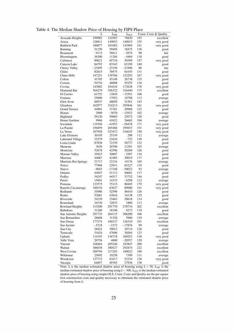
Table 4: The Median Shadow Price of Housing by FIPS Placeλ λ300 λOLS Const. Costs & Quality
Avocado Heights 199982 124583 78830 193 excellentAzusa 128811 149853 140915 155 very goodBaldwin Park 100877 161082 143994 141 very goodBanning 51250 59456 18475 136 goodBeaumont −9115 30411 −2974 98 fairBloomington 36300 11284 −4404 118 goodCalimesa 89621 65716 50389 157 very goodCanyon Lake 84793 83343 63199 140 goodCherry Valley −23495 −23156 −23496 88 fairChino 82615 76975 64193 131 goodChino Hills 147251 139766 132293 167 very goodColton 41705 45148 26738 135 goodCorona 54754 46098 45255 118 goodCovina 143002 181634 172628 178 very goodDiamond Bar 364279 356322 316440 175 excellentEl Cerrito 61752 12845 −33391 108 goodFontana 25090 17952 10798 112 averageGlen Avon 66937 48050 31561 143 goodGlendora 162977 324213 295846 161 very goodGrand Terrace 44901 37181 20968 122 goodHemet 2909 −5070 −12923 102 averageHighland 59120 59885 25072 129 goodHome Gardens 9966 41032 36665 104 averageIrwindale 119394 −41953 −58478 171 very goodLa Puente 156859 265466 195653 151 very goodLa Verne 187958 323472 316635 150 very goodLake Elsinore 30195 25339 298 112 averageLakeland Village 35279 23416 −723 130 goodLoma Linda 87038 72339 58737 132 goodMentone 3039 20700 12391 103 averageMontclair 52678 42596 50269 126 goodMoreno Valley 35823 30807 −2507 116 goodMurrieta 44067 42485 30019 117 goodMurrieta Hot Springs 21717 22154 19176 105 averageNorco 77968 23931 65227 119 goodNuevo −9043 −17348 −50023 93 averageOntario 44947 51113 40601 117 goodPedley 54247 44517 33752 144 goodPerris 15691 14333 −6298 112 averagePomona 123575 75115 80485 179 very goodRancho Cucamonga 100154 63627 80980 141 very goodRedlands 55086 52598 48410 126 goodRialto 52081 43816 16138 135 goodRiverside 34239 23463 20618 114 goodRomoland 24330 32833 1800 113 averageRowland Heights 315200 291770 278734 202 excellentRubidoux 31289 18196 8273 119 goodSan Antonio Heights 293735 264115 306200 168 excellentSan Bernardino 28608 31328 5960 119 averageSan Dimas 177574 160137 126319 191 excellentSan Jacinto −5218 −2372 −17876 99 averageSun City 28422 39013 10714 126 goodTemecula 51624 47696 30564 123 goodUpland 114193 136718 160253 138 very goodValle Vista 20756 4880 −20557 120 averageVincent 168464 205246 183847 200 excellentWalnut 386038 380527 292874 222 excellentWest Covina 209794 217203 189022 190 excellentWildomar 25692 19258 7399 111 averageWoodcrest 127715 63417 52234 136 very goodYucaipa 64857 49765 27936 138 goodNote: λ is the median estimated shadow price of housing using k = 50, λ300 is themedian estimated shadow price of housing using k = 300, λOLS is the median estimatedshadow price of housing using simple OLS, Const. Costs and Quality are the per squarefoot construction costs and quality necessary to eliminate the estimated shadow priceof housing from λ.
25
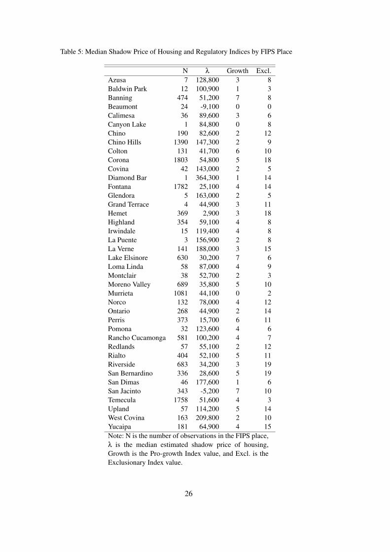
Table 5: Median Shadow Price of Housing and Regulatory Indices by FIPS Place
N λ Growth Excl.Azusa 7 128,800 3 8Baldwin Park 12 100,900 1 3Banning 474 51,200 7 8Beaumont 24 -9,100 0 0Calimesa 36 89,600 3 6Canyon Lake 1 84,800 0 8Chino 190 82,600 2 12Chino Hills 1390 147,300 2 9Colton 131 41,700 6 10Corona 1803 54,800 5 18Covina 42 143,000 2 5Diamond Bar 1 364,300 1 14Fontana 1782 25,100 4 14Glendora 5 163,000 2 5Grand Terrace 4 44,900 3 11Hemet 369 2,900 3 18Highland 354 59,100 4 8Irwindale 15 119,400 4 8La Puente 3 156,900 2 8La Verne 141 188,000 3 15Lake Elsinore 630 30,200 7 6Loma Linda 58 87,000 4 9Montclair 38 52,700 2 3Moreno Valley 689 35,800 5 10Murrieta 1081 44,100 0 2Norco 132 78,000 4 12Ontario 268 44,900 2 14Perris 373 15,700 6 11Pomona 32 123,600 4 6Rancho Cucamonga 581 100,200 4 7Redlands 57 55,100 2 12Rialto 404 52,100 5 11Riverside 683 34,200 3 19San Bernardino 336 28,600 5 19San Dimas 46 177,600 1 6San Jacinto 343 -5,200 7 10Temecula 1758 51,600 4 3Upland 57 114,200 5 14West Covina 163 209,800 2 10Yucaipa 181 64,900 4 15Note: N is the number of observations in the FIPS place,λ is the median estimated shadow price of housing,Growth is the Pro-growth Index value, and Excl. is theExclusionary Index value.
26
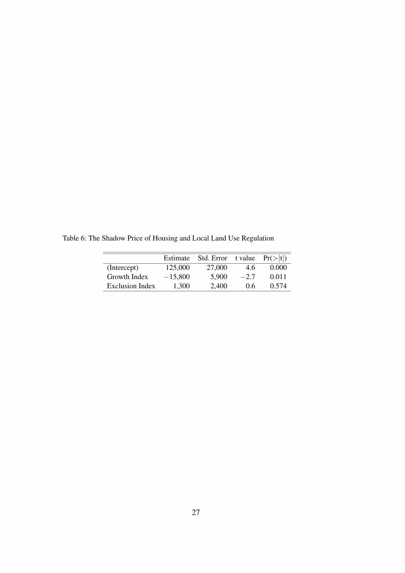
Table 6: The Shadow Price of Housing and Local Land Use Regulation
Estimate Std. Error t value Pr(>|t|)(Intercept) 125,000 27,000 4.6 0.000Growth Index −15,800 5,900 −2.7 0.011Exclusion Index 1,300 2,400 0.6 0.574
27