raven 3 examples - convergent · raven examples march 6, 2013 page 11 the resulting plot is shown...

Convergent Manufacturing Technologies Inc.

6190 Agronomy Road, Suite 403, Vancouver, British Columbia, Canada, V6T 1Z3 Tel: 604-822-9682, Fax: 604-822-9659, [email protected], www.convergent.ca

2013

RAVEN 3 Examples

Convergent Manufacturing Technologies Inc.

6190 Agronomy Road, Suite 403, Vancouver, British Columbia, Canada, V6T 1Z3 Tel: 604-822-9682, Fax: 604-822-9659, [email protected], www.convergent.ca

RAVEN Examples

March 6, 2013 Page 1

Contents

RAVEN EXAMPLES ....................................................................................................... 2

Example 1a: Create a basic Virtual Material Module simulation ............................................2

Example 1b: Create a plot from a basic Virtual Material Model simulation ...........................7

Example 1c: Modifying an existing simulation and using the cycle editor .........................14

Example 1d: Basic simulation the easy way .........................................................................19

Example 2: Compare 1 material with two cycles ..................................................................21

Example 3: Compare two materials with a single cure cycle ...............................................31

Example 4: Create a thermal profile of a thin laminate.........................................................36

Example 5: Create a thermal profile of a thick laminate .......................................................47

Example 6: Import Data ..........................................................................................................51

Example 7: Create a thermal profile of a 2D flat laminate ....................................................61

Example 8: Compare 2D and 1D thermal profile studies ......................................................67

Example 9: Process Maps ......................................................................................................75

RAVEN Examples


RAVEN Examples The following examples have been created to expose users to the features of RAVEN Virtual Material Module and the RAVEN Thermal Profile Module. The examples are intended to be performed in order, as the each builds on the skills and familiarity of the previous.

Syntax note: When referring to a menu item, the convention is “Main Menu Item”|”Sub Menu Item”. For example, the menu item found under the “File” main menu called “Save” is referred to as File|Save.

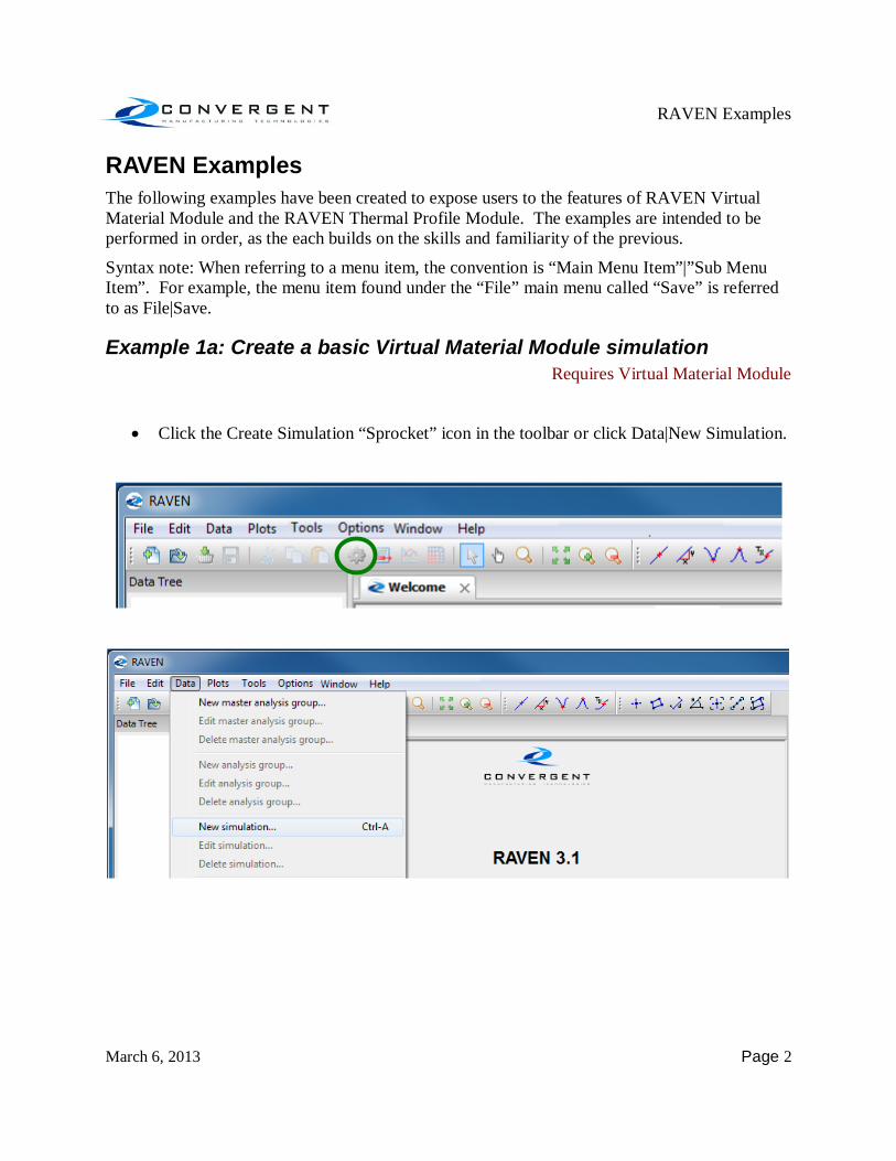
Example 1a: Create a basic Virtual Material Module simulation Requires Virtual Material Module

Click the Create Simulation “Sprocket” icon in the toolbar or click Data|New Simulation.

RAVEN Examples


The “Select Simulation Type” dialog pops up. Select “Virtual Material Simulation”.

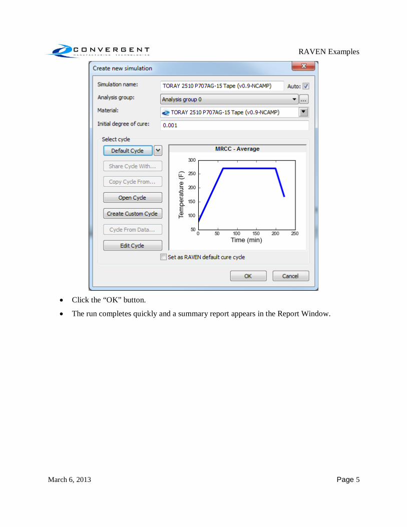
The Create new simulation dialog box pops up.

RAVEN Examples


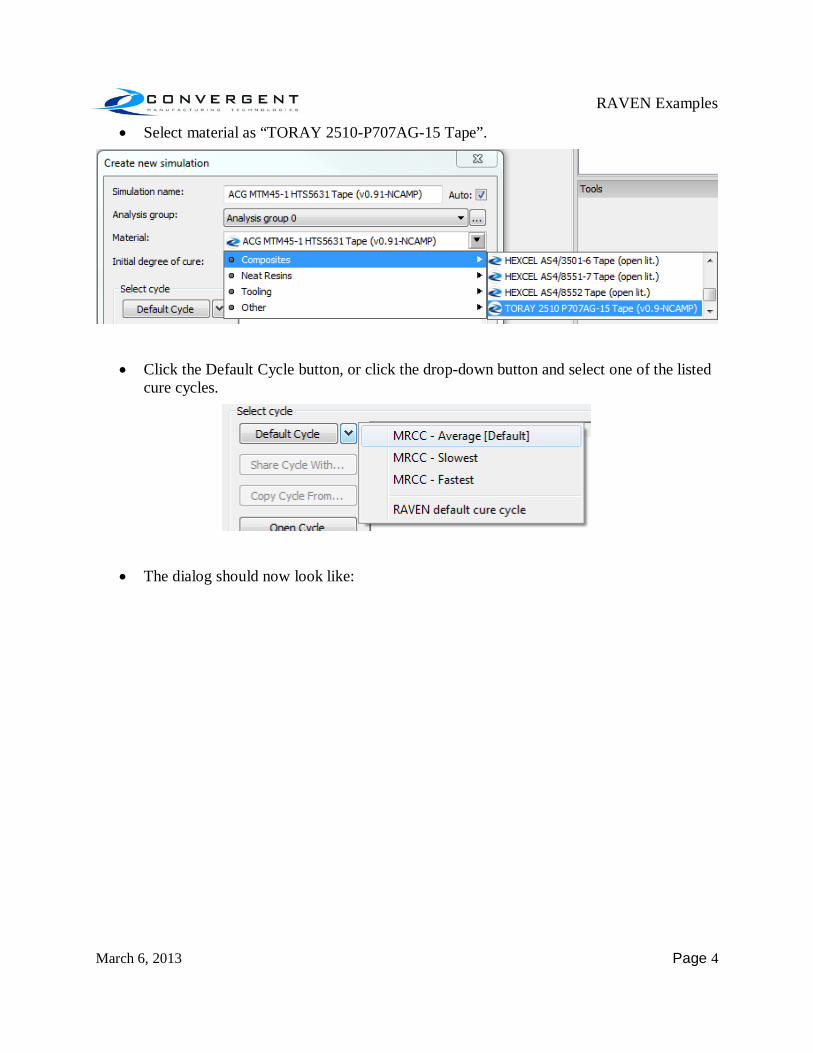
Select material as “TORAY 2510-P707AG-15 Tape”.

Click the Default Cycle button, or click the drop-down button and select one of the listed cure cycles.

The dialog should now look like:

RAVEN Examples


Click the “OK” button.

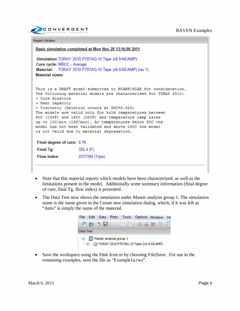
The run completes quickly and a summary report appears in the Report Window.

RAVEN Examples


Note that this material reports which models have been characterized, as well as the

limitations present in the model. Additionally some summary information (final degree of cure, final Tg, flow index) is presented.

The Data Tree now shows the simulation under Master analysis group 1. The simulation name is the name given in the Create new simulation dialog, which, if it was left as “Auto” is simply the name of the material.

Save the workspace using the Disk Icon or by choosing File|Save. For use in the

remaining examples, save the file as “Example1a.rws”.

RAVEN Examples


Example 1b: Create a plot from a basic Virtual Material Model simulation

Requires Virtual Material Module

Open the “Example1a.rws” file created in Example 1a.

Click the Create Plot button, or select Plots|New Plot...

RAVEN Examples


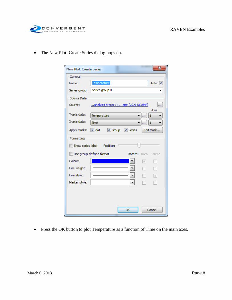
The New Plot: Create Series dialog pops up.

Press the OK button to plot Temperature as a function of Time on the main axes.

RAVEN Examples


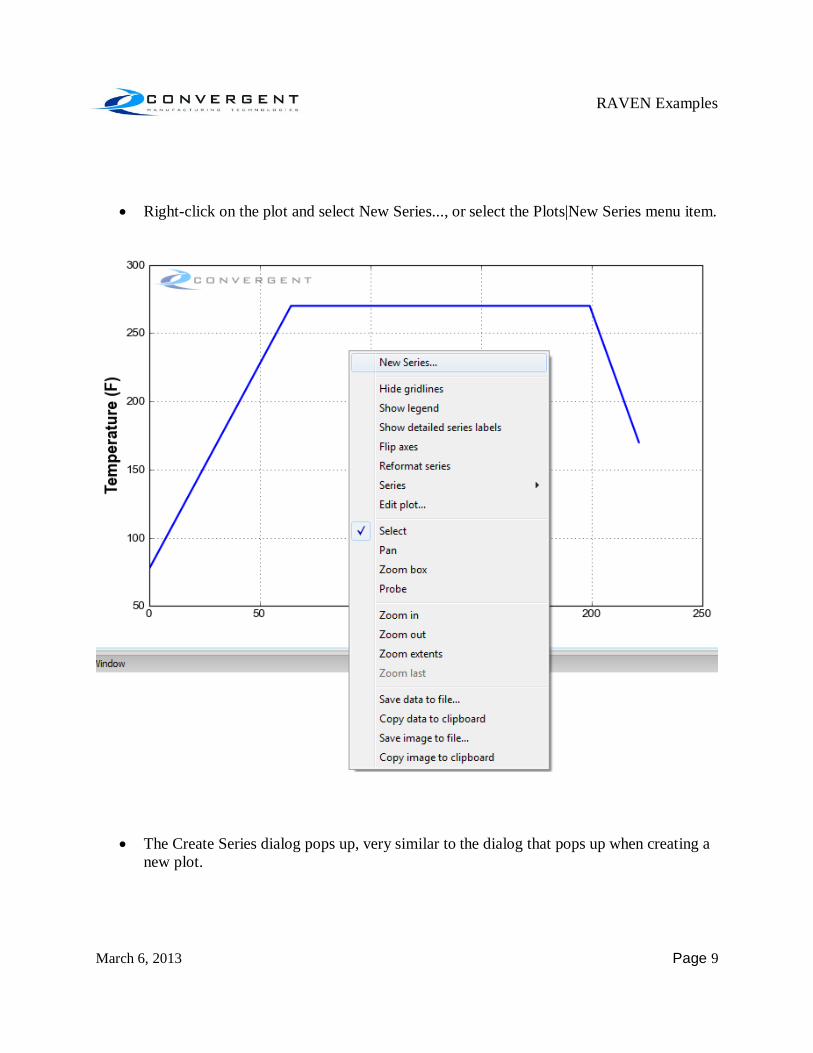
Right-click on the plot and select New Series..., or select the Plots|New Series menu item.

The Create Series dialog pops up, very similar to the dialog that pops up when creating a new plot.

RAVEN Examples


Choose “Degree of Cure” from the Y-axis data drop-down and make sure that it is plotted on Y-axis 2.

RAVEN Examples


The resulting plot is shown below:

You can access a number of plot manipulation tools from the toolbar including: Pan,

Zoom, and Probe

The pan tool can be used to drag the plot around.

The zoom tool allows you to draw a window around portions of the plot to zoom in

The zoom can also be reset with the zoom extents button.

The zoom can be increased or decreased stepwise using the increase/decrease zoom buttons.

RAVEN Examples


The probe tool allows you to determine the value at a point beneath the probe. The value is reported in the report window.

You can also probe for a slope , local maximum or local minimum

These tools are also available by right-clicking the plot. Further, you can show/hide the gridlines, show/hide the legend, show/hide detailed series labels, and export the plot image and data in various ways.

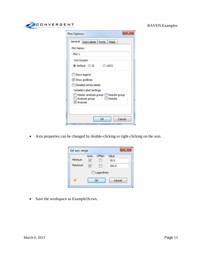
Various plot parameters can be adjusted by selecting the “Edit plot...” item (which is also

available via right-clicking the plot, right-clicking the plot name in the plot tree or by selecting Plots|Edit Plot.

RAVEN Examples


Axis properties can be changed by double-clicking or right-clicking on the axis.

Save the workspace as Example1b.rws.

RAVEN Examples


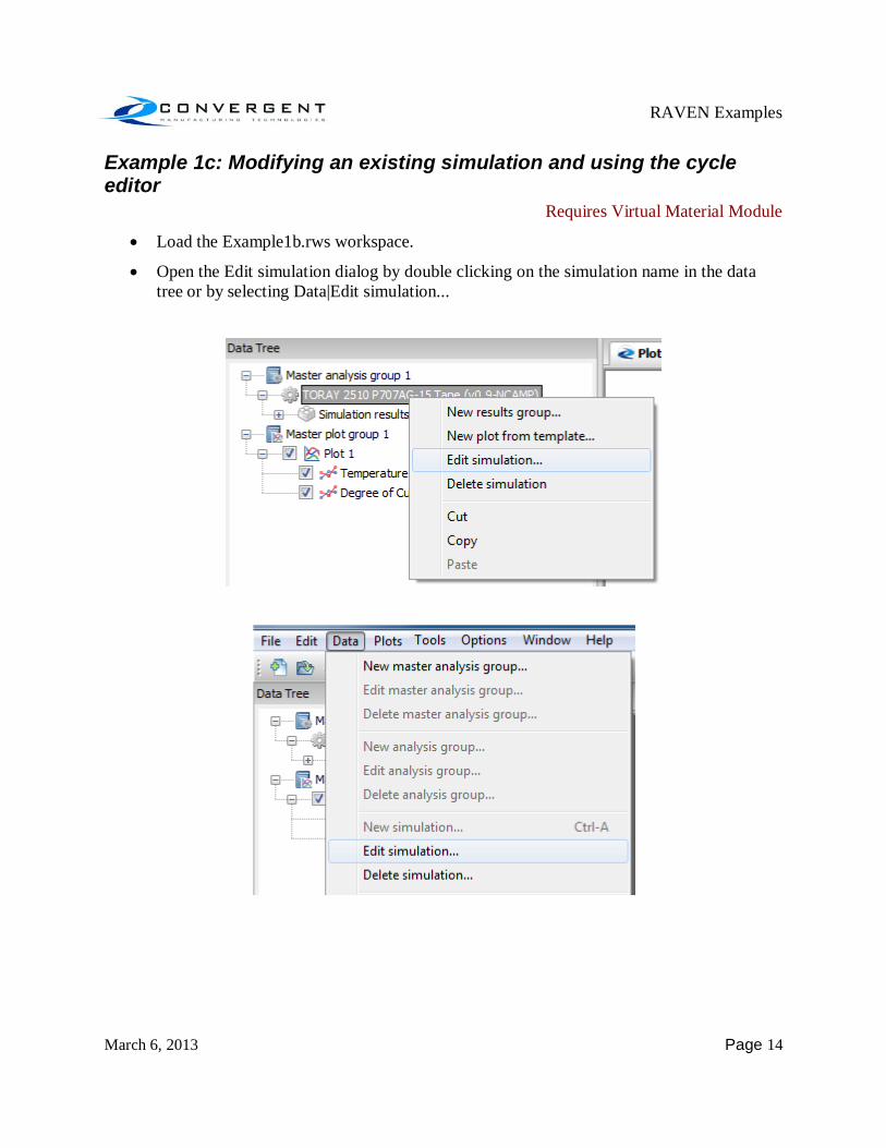
Example 1c: Modifying an existing simulation and using the cycle editor

Requires Virtual Material Module

Load the Example1b.rws workspace.

Open the Edit simulation dialog by double clicking on the simulation name in the data tree or by selecting Data|Edit simulation...

RAVEN Examples


In the Edit simulation dialog, you can change the simulation name, the material involved, or the cycle.

Click the edit cycle button.

RAVEN Examples


The Cure Cycle Editor dialog pops up:

Change the initial ramp temperature target to 175 F and the initial ramp rate to 2.0 F/min

by double clicking the numbers in the list, typing in the new numbers, then pressing the Enter key.

In a similar manner, change the hold time to 60 minutes.

With the 60 minute hold selected, click the “<<Ramp” button to add a second ramp to the cure cycle.

Change its ramp target and rate to 270 F at 3.0 F/min.

Add a 60 minute hold by clicking the “<<Hold” button.

RAVEN Examples


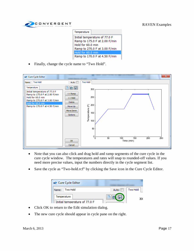
Finally, change the cycle name to “Two Hold”.

Note that you can also click and drag hold and ramp segments of the cure cycle in the

cure cycle window. The temperatures and rates will snap to rounded-off values. If you need more precise values, input the numbers directly in the cycle segment list.

Save the cycle as “Two-hold.rcf” by clicking the Save icon in the Cure Cycle Editor.

Click OK to return to the Edit simulation dialog.

The new cure cycle should appear in cycle pane on the right.

RAVEN Examples


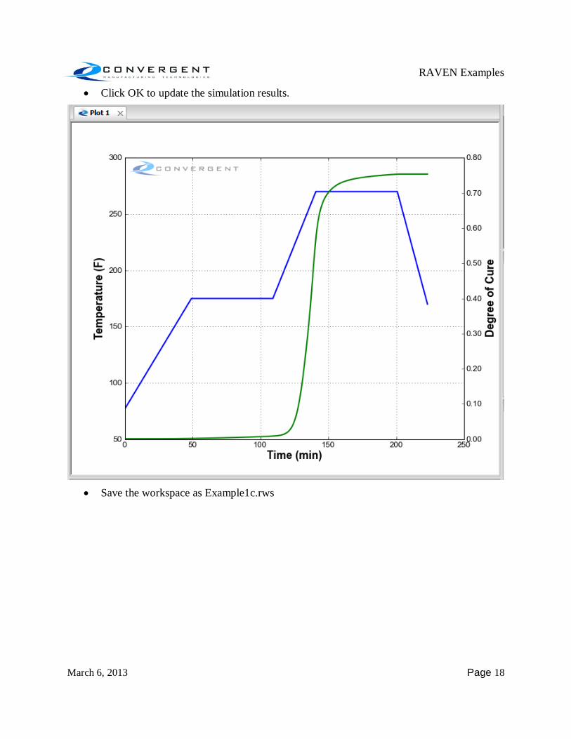
Click OK to update the simulation results.

Save the workspace as Example1c.rws

RAVEN Examples


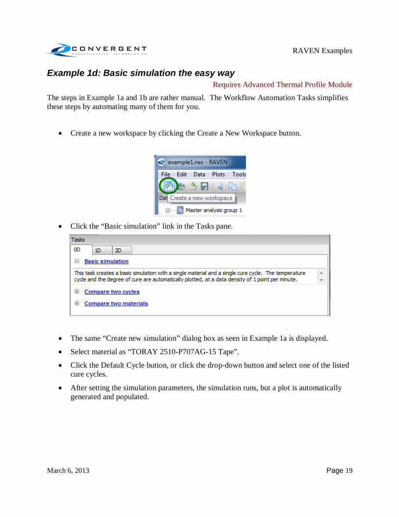
Example 1d: Basic simulation the easy way Requires Advanced Thermal Profile Module

The steps in Example 1a and 1b are rather manual. The Workflow Automation Tasks simplifies these steps by automating many of them for you.

Create a new workspace by clicking the Create a New Workspace button.

Click the “Basic simulation” link in the Tasks pane.

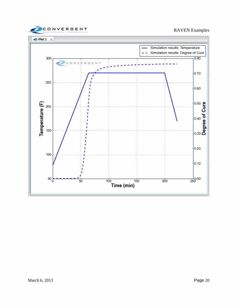
The same “Create new simulation” dialog box as seen in Example 1a is displayed.

Select material as “TORAY 2510-P707AG-15 Tape”.

Click the Default Cycle button, or click the drop-down button and select one of the listed cure cycles.

After setting the simulation parameters, the simulation runs, but a plot is automatically generated and populated.

RAVEN Examples


RAVEN Examples


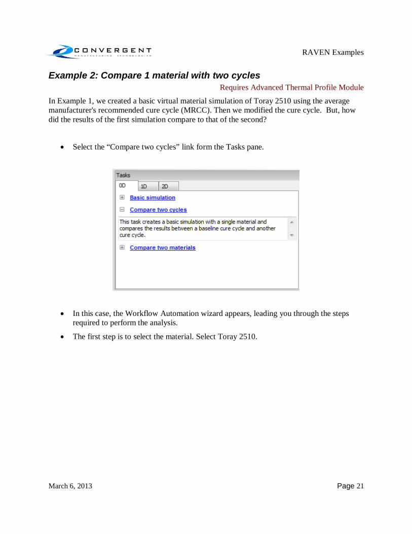
Example 2: Compare 1 material with two cycles Requires Advanced Thermal Profile Module

In Example 1, we created a basic virtual material simulation of Toray 2510 using the average manufacturer's recommended cure cycle (MRCC). Then we modified the cure cycle. But, how did the results of the first simulation compare to that of the second?

Select the “Compare two cycles” link form the Tasks pane.

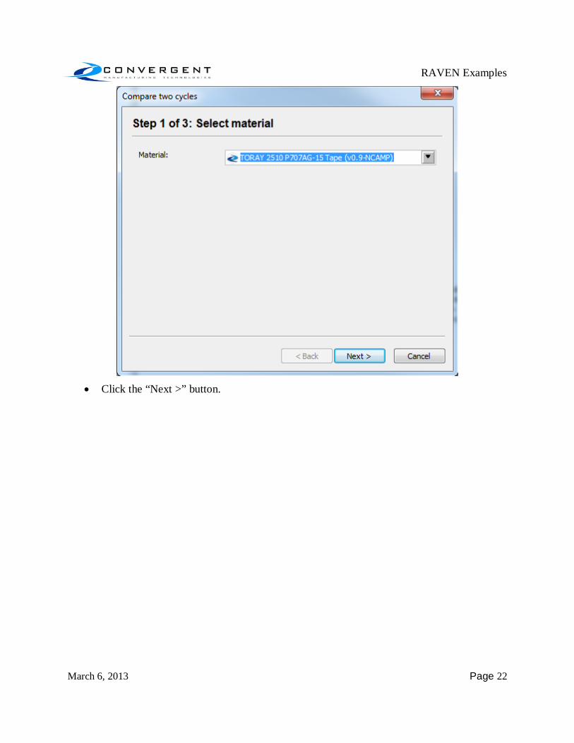
In this case, the Workflow Automation wizard appears, leading you through the steps required to perform the analysis.

The first step is to select the material. Select Toray 2510.

RAVEN Examples


Click the “Next >” button.

RAVEN Examples


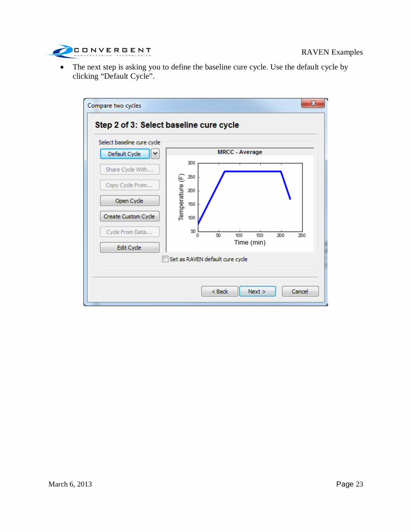
The next step is asking you to define the baseline cure cycle. Use the default cycle by clicking “Default Cycle”.

RAVEN Examples


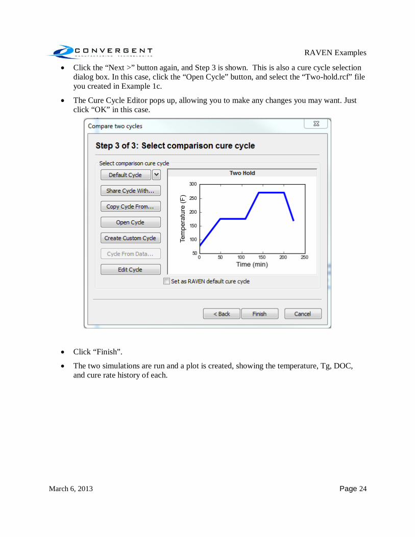
Click the “Next >” button again, and Step 3 is shown. This is also a cure cycle selection dialog box. In this case, click the “Open Cycle” button, and select the “Two-hold.rcf” file you created in Example 1c.

The Cure Cycle Editor pops up, allowing you to make any changes you may want. Just click “OK” in this case.

Click “Finish”.

The two simulations are run and a plot is created, showing the temperature, Tg, DOC, and cure rate history of each.

RAVEN Examples


The plot is a little cluttered. Turn off the legend by right-clicking on an empty area of the

plot, and selecting “Hide Legend”.

Individual series or groups of series can be turned on or off by checking or unchecking the appropriate checkboxes in the plot tree. Turn the Tg group off by unchecking it.

RAVEN Examples


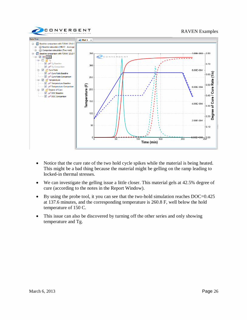
Notice that the cure rate of the two hold cycle spikes while the material is being heated. This might be a bad thing because the material might be gelling on the ramp leading to locked-in thermal stresses.

We can investigate the gelling issue a little closer. This material gels at 42.5% degree of cure (according to the notes in the Report Window).

By using the probe tool, it you can see that the two-hold simulation reaches DOC=0.425 at 137.6 minutes, and the corresponding temperature is 260.8 F, well below the hold temperature of 150 C.

This issue can also be discovered by turning off the other series and only showing temperature and Tg.

RAVEN Examples


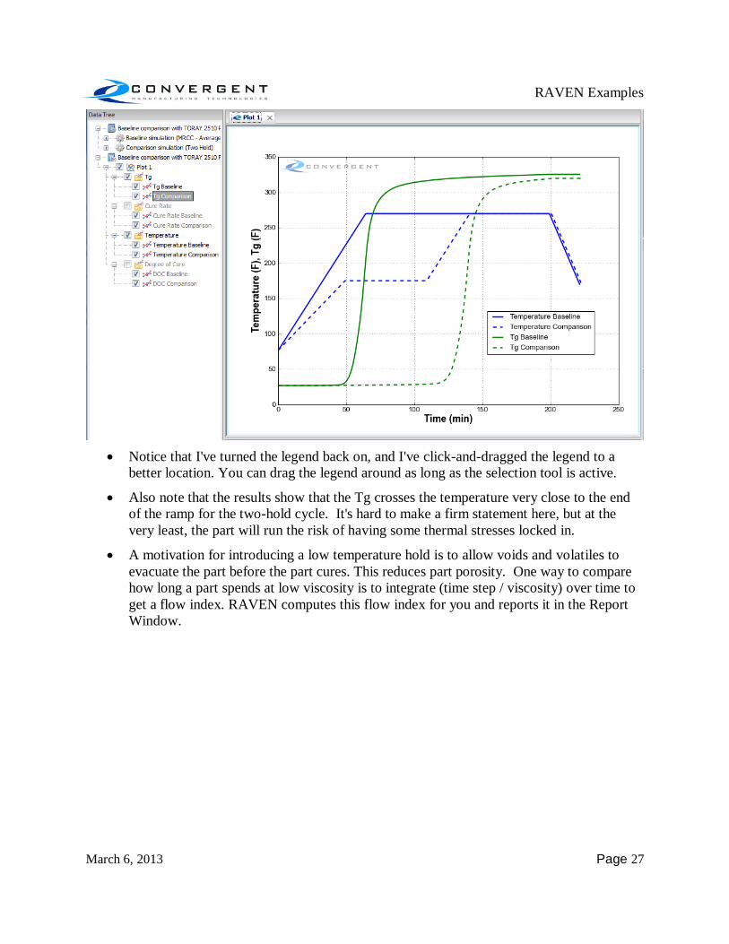
Notice that I've turned the legend back on, and I've click-and-dragged the legend to a

better location. You can drag the legend around as long as the selection tool is active.

Also note that the results show that the Tg crosses the temperature very close to the end of the ramp for the two-hold cycle. It's hard to make a firm statement here, but at the very least, the part will run the risk of having some thermal stresses locked in.

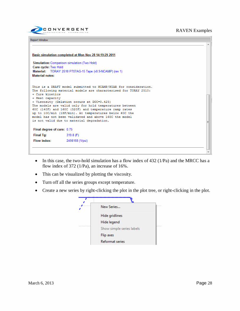
A motivation for introducing a low temperature hold is to allow voids and volatiles to evacuate the part before the part cures. This reduces part porosity. One way to compare how long a part spends at low viscosity is to integrate (time step / viscosity) over time to get a flow index. RAVEN computes this flow index for you and reports it in the Report Window.

RAVEN Examples


In this case, the two-hold simulation has a flow index of 432 (1/Pa) and the MRCC has a

flow index of 372 (1/Pa), an increase of 16%.

This can be visualized by plotting the viscosity.

Turn off all the series groups except temperature.

Create a new series by right-clicking the plot in the plot tree, or right-clicking in the plot.

RAVEN Examples


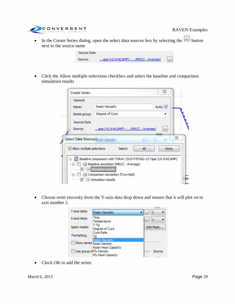
In the Create Series dialog, open the select data sources box by selecting the button next to the source name

Click the Allow multiple selections checkbox and select the baseline and comparison simulation results

Choose resin viscosity from the Y-axis data drop down and ensure that it will plot on to axis number 2.

Clock OK to add the series

RAVEN Examples


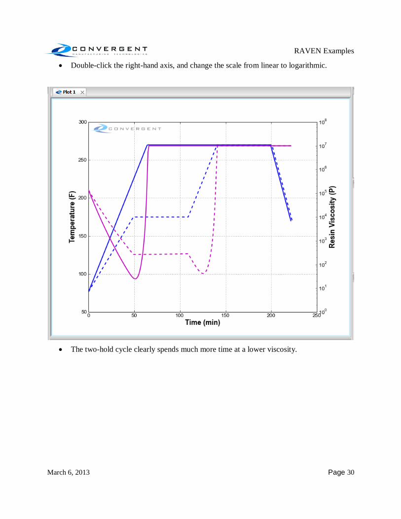
Double-click the right-hand axis, and change the scale from linear to logarithmic.

The two-hold cycle clearly spends much more time at a lower viscosity.

RAVEN Examples


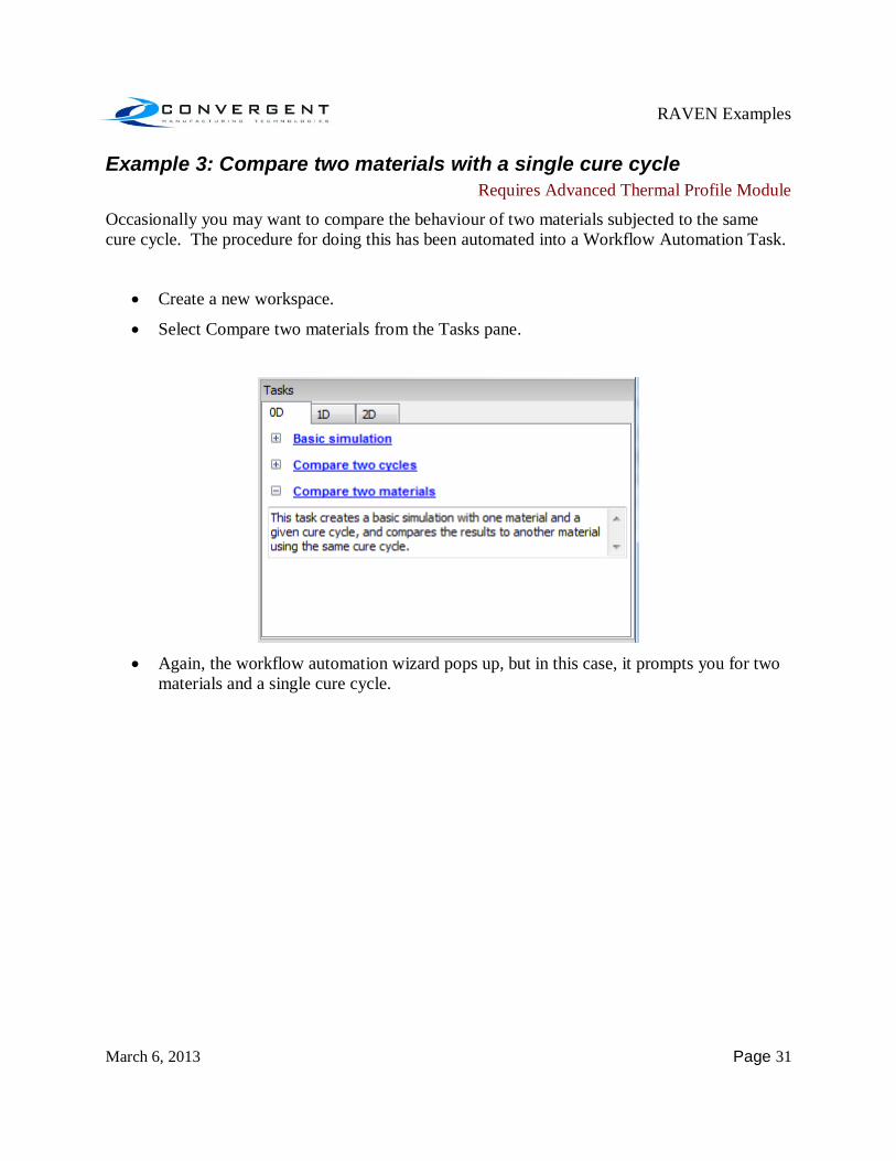
Example 3: Compare two materials with a single cure cycle Requires Advanced Thermal Profile Module

Occasionally you may want to compare the behaviour of two materials subjected to the same cure cycle. The procedure for doing this has been automated into a Workflow Automation Task.

Create a new workspace.

Select Compare two materials from the Tasks pane.

Again, the workflow automation wizard pops up, but in this case, it prompts you for two

materials and a single cure cycle.

RAVEN Examples


Select Toray 2510 as the first material.

RAVEN Examples


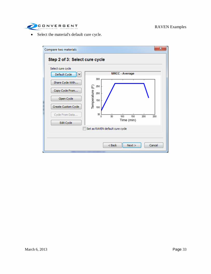
Select the material's default cure cycle.

RAVEN Examples


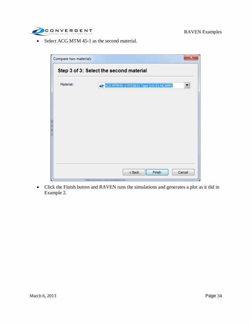
Select ACG MTM 45-1 as the second material.

Click the Finish button and RAVEN runs the simulations and generates a plot as it did in

Example 2.

RAVEN Examples


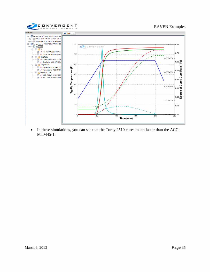
In these simulations, you can see that the Toray 2510 cures much faster than the ACG

MTM45-1.

RAVEN Examples


Example 4: Create a thermal profile of a thin laminate Requires Advanced Thermal Profile Module

Open a new workspace by clicking the New button.

The easiest way to perform thermal analyses of laminates is to use the “Thermal Profile Study” workflow automation task. It is located under the 1D tab in the task pane

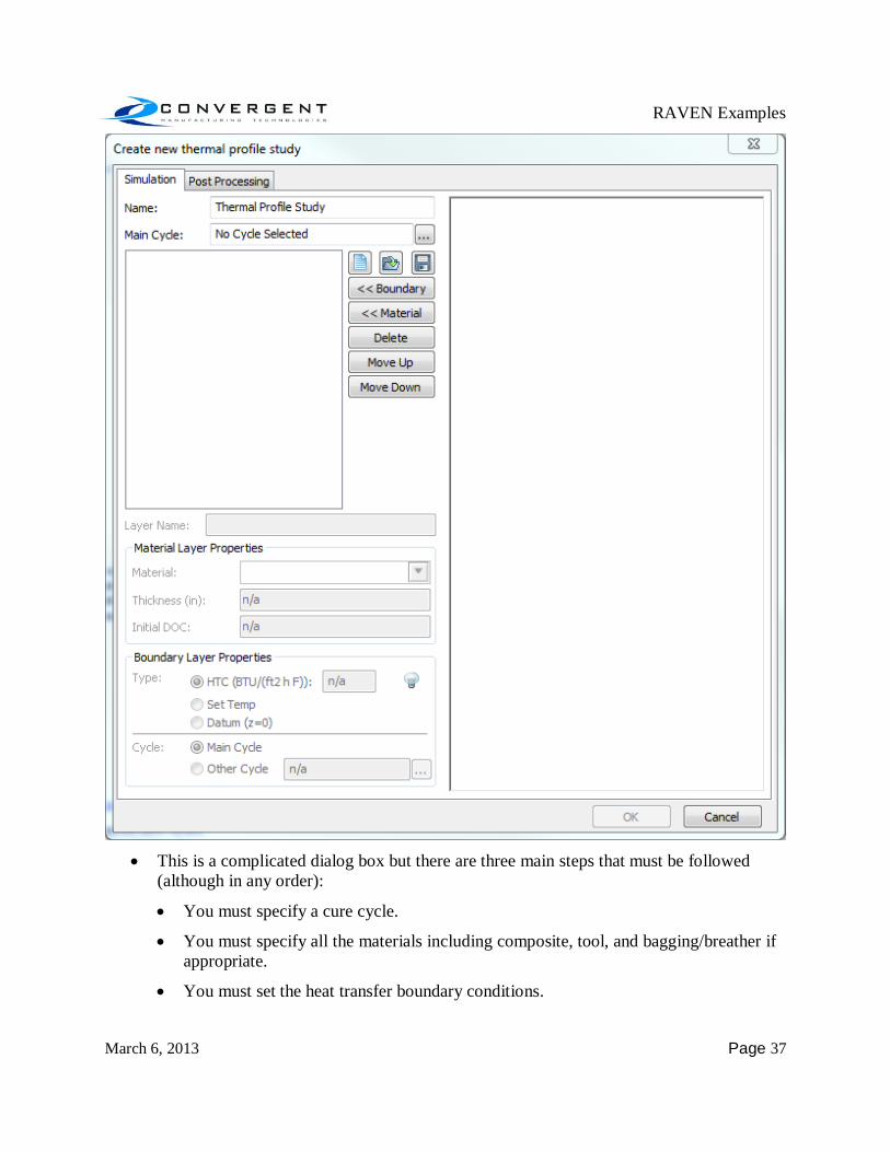
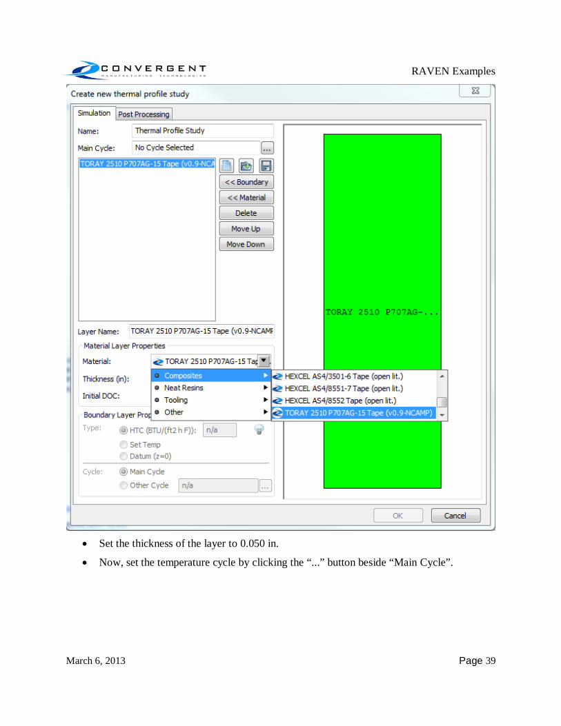
The Create new thermal profile study dialog is raised.

RAVEN Examples


This is a complicated dialog box but there are three main steps that must be followed

(although in any order):

You must specify a cure cycle.

You must specify all the materials including composite, tool, and bagging/breather if appropriate.

You must set the heat transfer boundary conditions.

RAVEN Examples


Following these three steps is the minimum required, everything beyond that is refinement.

First, specify the material. In this case we will use 8 plies of Toray 2510 (at 0.006” = 0.152mm per ply). For a 1D analysis, RAVEN only accepts total thickness as an input, not the number of plies.

Click the “<< Material” button to add a material layer.

Change the material to Toray 2510.

RAVEN Examples


Set the thickness of the layer to 0.050 in.

Now, set the temperature cycle by clicking the “...” button beside “Main Cycle”.

RAVEN Examples


Select the default MRCC from the Create new cycle dialog.

Add a steel tool (0.5 in. thick) and some breather cloth (1 ply @ 0.03 in per ply) to the analysis too using the “<< Material” button, and the “Move Up” and “Move Down” buttons as necessary.

Next we need to establish some boundary conditions.

First, we'll put a datum (the location of z=0) between the part and the tool so that everything is correctly plotted with respect to the tool-part interface.

Insert a boundary with the “<< Boundary” button, use the “Move Up” and “Move Down” buttons to position the boundary between the part and the tool.

Change the boundary type to Datum (z=0).

RAVEN Examples


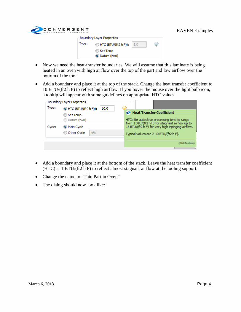
Now we need the heat-transfer boundaries. We will assume that this laminate is being

heated in an oven with high airflow over the top of the part and low airflow over the bottom of the tool.

Add a boundary and place it at the top of the stack. Change the heat transfer coefficient to 10 BTU/(ft2 h F) to reflect high airflow. If you hover the mouse over the light bulb icon, a tooltip will appear with some guidelines on appropriate HTC values.

Add a boundary and place it at the bottom of the stack. Leave the heat transfer coefficient (HTC) at 1 BTU/(ft2 h F) to reflect almost stagnant airflow at the tooling support.

Change the name to “Thin Part in Oven”.

The dialog should now look like:

RAVEN Examples


Click the OK button, and wait a little bit.

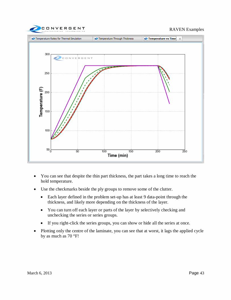
The temperature vs time plot generated.

RAVEN Examples


You can see that despite the thin part thickness, the part takes a long time to reach the hold temperature.

Use the checkmarks beside the ply groups to remove some of the clutter.

Each layer defined in the problem set-up has at least 9 data-point through the thickness, and likely more depending on the thickness of the layer.

You can turn off each layer or parts of the layer by selectively checking and unchecking the series or series groups.

If you right-click the series groups, you can show or hide all the series at once.

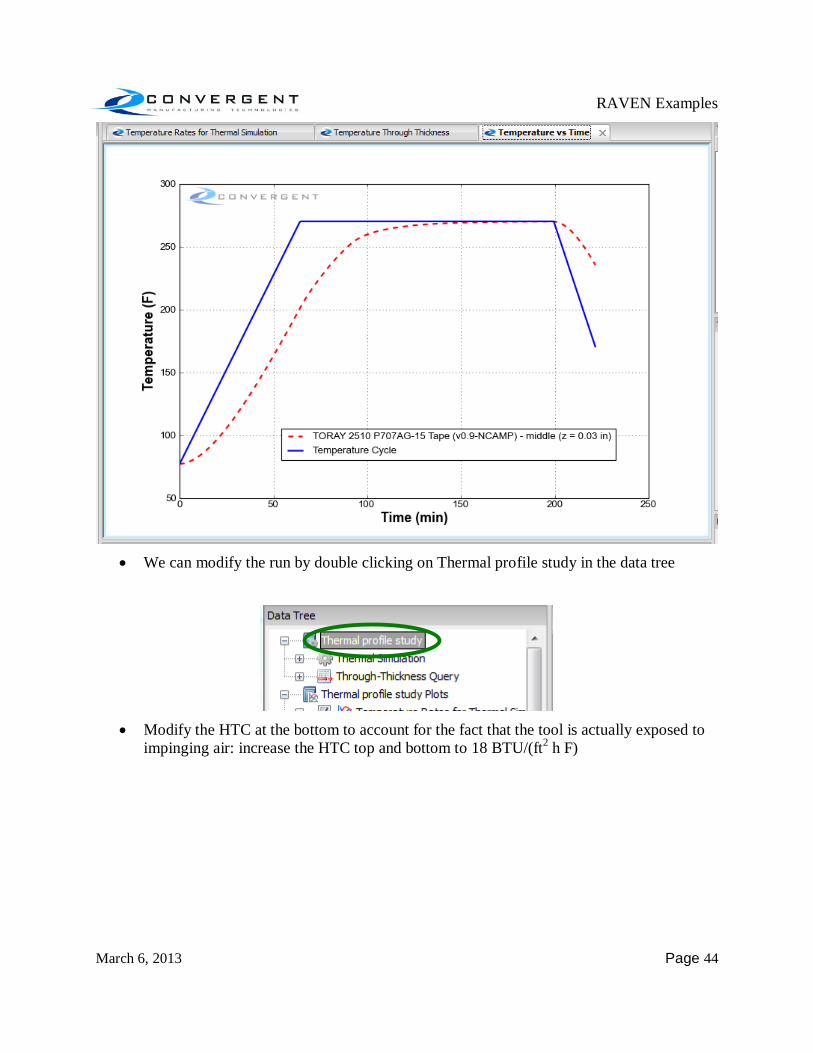
Plotting only the centre of the laminate, you can see that at worst, it lags the applied cycle by as much as 70 °F!

RAVEN Examples


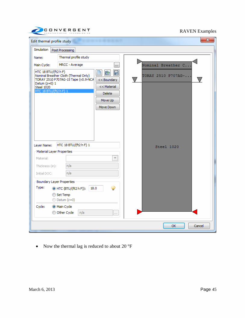
We can modify the run by double clicking on Thermal profile study in the data tree

Modify the HTC at the bottom to account for the fact that the tool is actually exposed to

impinging air: increase the HTC top and bottom to 18 BTU/(ft2 h F)

RAVEN Examples


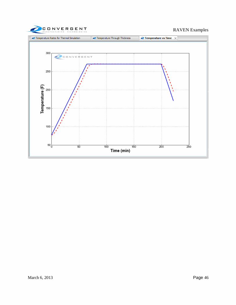
Now the thermal lag is reduced to about 20 °F

RAVEN Examples


RAVEN Examples


Example 5: Create a thermal profile of a thick laminate Requires Advanced Thermal Profile module

Create a new workspace by clicking the “New” button.

This time, create a thick laminate with the following stack sequence and boundary conditions: 10 BTU/(ft2 h F)HTC on the top surface 0.03 in thick breather cloth 30 plies Toray 2510 (0.18 in.) 0.375 in. steel tooling 3.5 BTU/(ft2 h F)on the bottom

RAVEN Examples


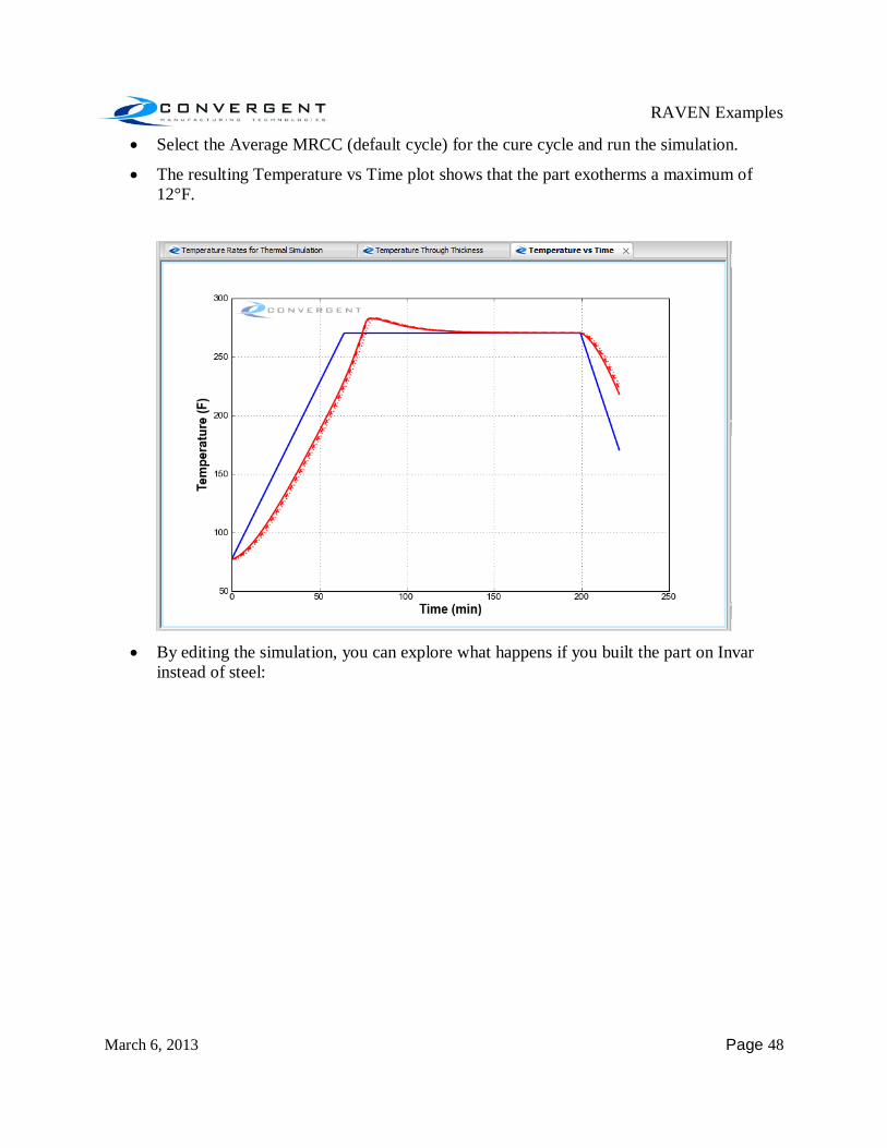
Select the Average MRCC (default cycle) for the cure cycle and run the simulation.

The resulting Temperature vs Time plot shows that the part exotherms a maximum of 12°F.

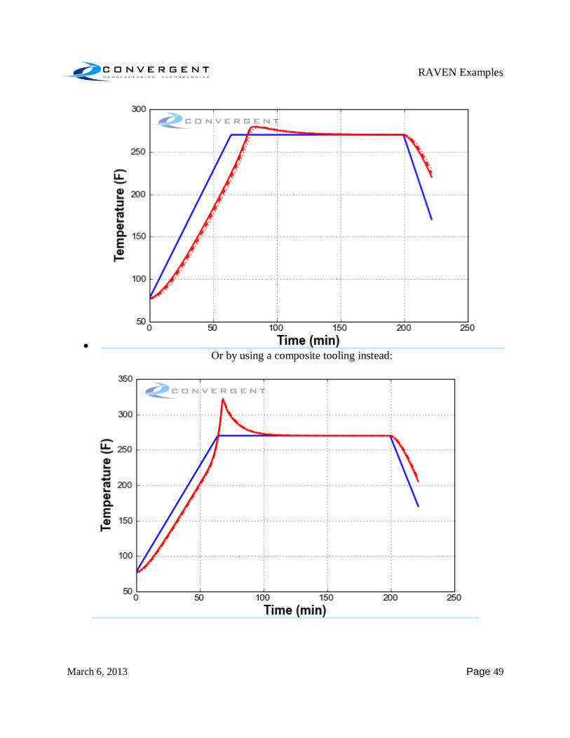
By editing the simulation, you can explore what happens if you built the part on Invar

instead of steel:

RAVEN Examples


Or by using a composite tooling instead:

RAVEN Examples


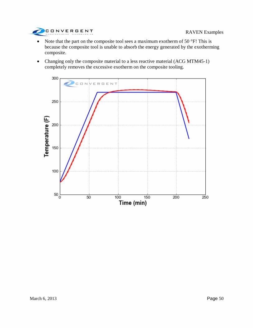
Note that the part on the composite tool sees a maximum exotherm of 50 °F! This is because the composite tool is unable to absorb the energy generated by the exotherming composite.

Changing only the composite material to a less reactive material (ACG MTM45-1) completely removes the excessive exotherm on the composite tooling.

RAVEN Examples


Example 6: Import Data Requires Advanced Thermal Profile module

Create a new workspace using the “New” button.

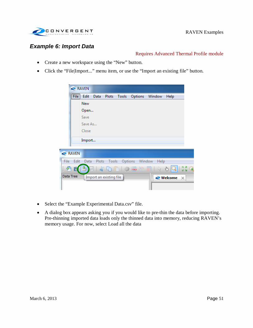
Click the “File|Import...” menu item, or use the “Import an existing file” button.

Select the “Example Experimental Data.csv” file.

A dialog box appears asking you if you would like to pre-thin the data before importing. Pre-thinning imported data loads only the thinned data into memory, reducing RAVEN’s memory usage. For now, select Load all the data

RAVEN Examples


Once the data is loaded, the Manage Imported Data dialog box will appear. In this dialog, RAVEN will attempt to assign a data type and unit to each imported column of data based on the column heading. Confirm that the first column is time in minutes and all the others are thermocouple temperature data at various positions, in ˚F. Click OK

RAVEN will then ask if you would like to thin the imported data. In contrast to Pre-thinning, thinning the data at this stage does not destroy the original data, but filters what is visible to the user. One immediate benefit of thinning the data is that the plots redraw, pan, and zoom much faster. Click “Yes”.

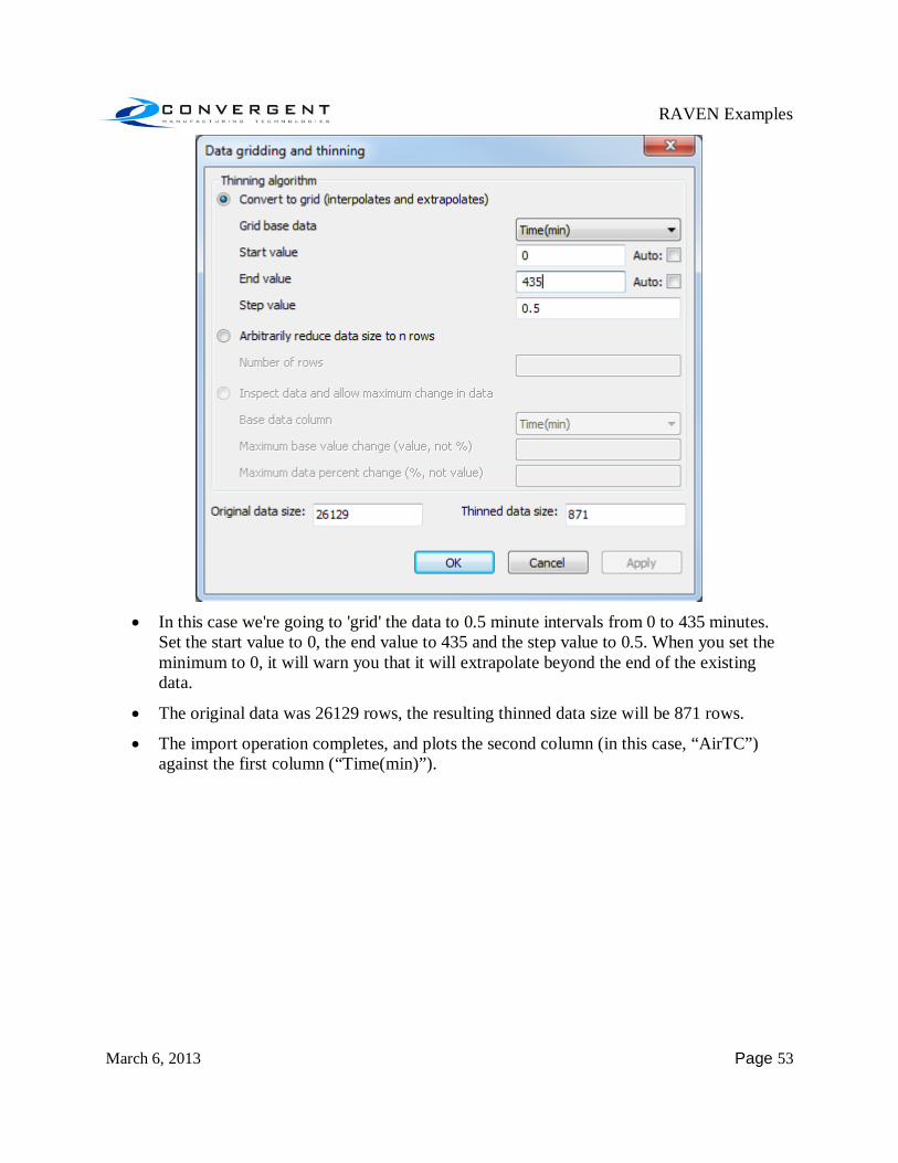
The Data gridding and thinning dialog appears.

RAVEN Examples


In this case we're going to 'grid' the data to 0.5 minute intervals from 0 to 435 minutes.

Set the start value to 0, the end value to 435 and the step value to 0.5. When you set the minimum to 0, it will warn you that it will extrapolate beyond the end of the existing data.

The original data was 26129 rows, the resulting thinned data size will be 871 rows.

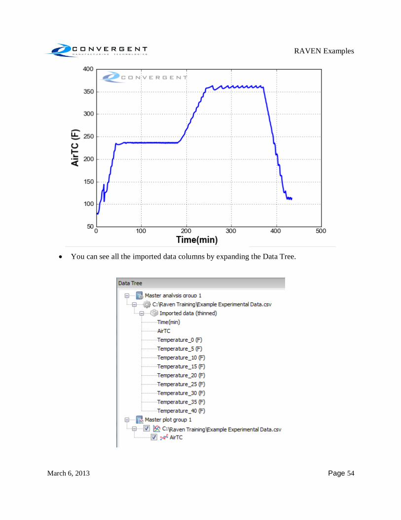
The import operation completes, and plots the second column (in this case, “AirTC”) against the first column (“Time(min)”).

RAVEN Examples


You can see all the imported data columns by expanding the Data Tree.

RAVEN Examples


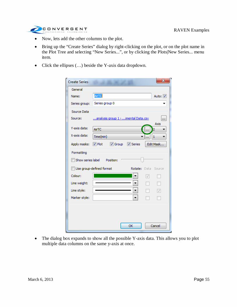
Now, lets add the other columns to the plot.

Bring up the “Create Series” dialog by right-clicking on the plot, or on the plot name in the Plot Tree and selecting “New Series...”, or by clicking the Plots|New Series... menu item.

Click the ellipses (…) beside the Y-axis data dropdown.

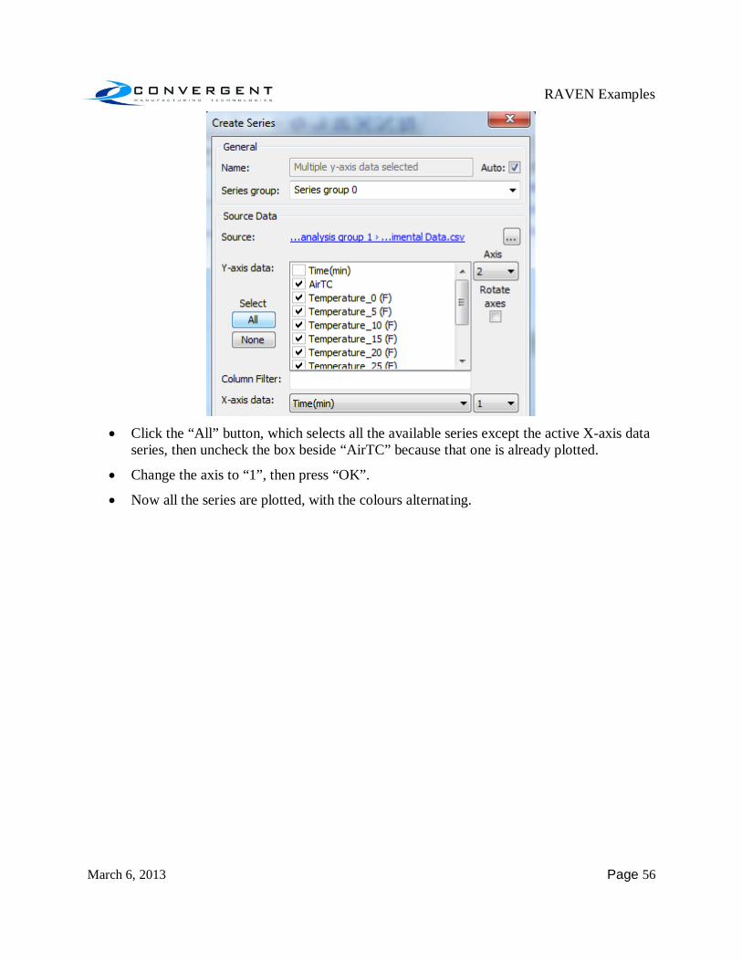
The dialog box expands to show all the possible Y-axis data. This allows you to plot

multiple data columns on the same y-axis at once.

RAVEN Examples


Click the “All” button, which selects all the available series except the active X-axis data

series, then uncheck the box beside “AirTC” because that one is already plotted.

Change the axis to “1”, then press “OK”.

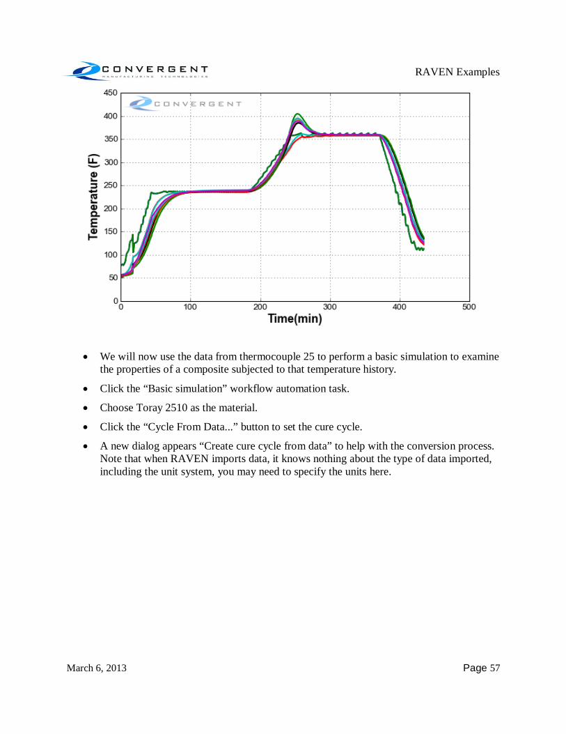
Now all the series are plotted, with the colours alternating.

RAVEN Examples


We will now use the data from thermocouple 25 to perform a basic simulation to examine the properties of a composite subjected to that temperature history.

Click the “Basic simulation” workflow automation task.

Choose Toray 2510 as the material.

Click the “Cycle From Data...” button to set the cure cycle.

A new dialog appears “Create cure cycle from data” to help with the conversion process. Note that when RAVEN imports data, it knows nothing about the type of data imported, including the unit system, you may need to specify the units here.

RAVEN Examples


Change the temperature source to “Temperature_25 (F)” and click OK.

The imported cure cycle is shown in the “Create new simulation” dialog.

Click “OK”.

RAVEN Examples


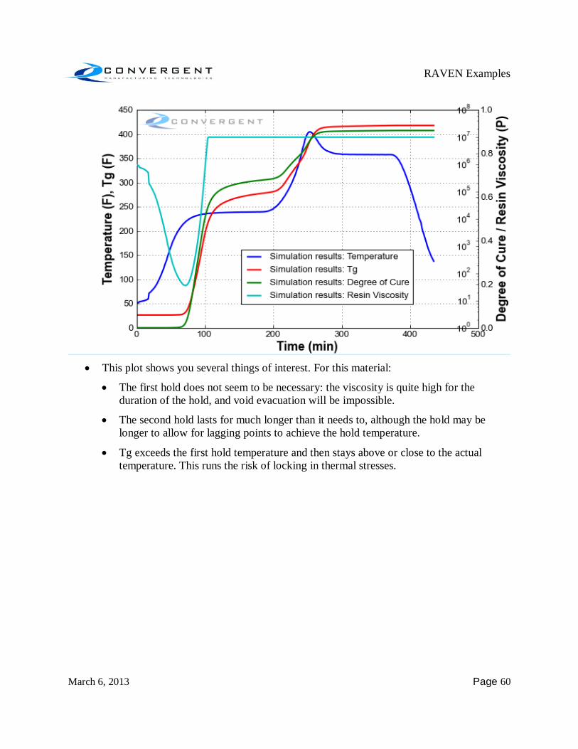
Add Tg and viscosity to the plot, changing colours and linetypes as needed.

RAVEN Examples


This plot shows you several things of interest. For this material:

The first hold does not seem to be necessary: the viscosity is quite high for the duration of the hold, and void evacuation will be impossible.

The second hold lasts for much longer than it needs to, although the hold may be longer to allow for lagging points to achieve the hold temperature.

Tg exceeds the first hold temperature and then stays above or close to the actual temperature. This runs the risk of locking in thermal stresses.

RAVEN Examples


Example 7: Create a thermal profile of a 2D flat laminate Create a new workspace using the “New” button.

Switch to SI units by going to Options | Preferences… | Units

To create a 2D thermal profile, select “2D dynamic template” under the 2D tab in the Tasks pane.

Dynamic templates are a set of pre-generated geometries which are representative of

typical features found in composite parts. RAVEN generates a 2D finite element mesh of the part geometry once the dimensions of the dynamic templates are specified. By contrast, static templates have pre-defined, fixed meshes where their geometry cannot be changed. Static templates are typically generated by a customer’s request and can include custom 2D features of the part.

By selecting “2D dynamic template”, the 2D dynamic template dialog is raised.

RAVEN Examples


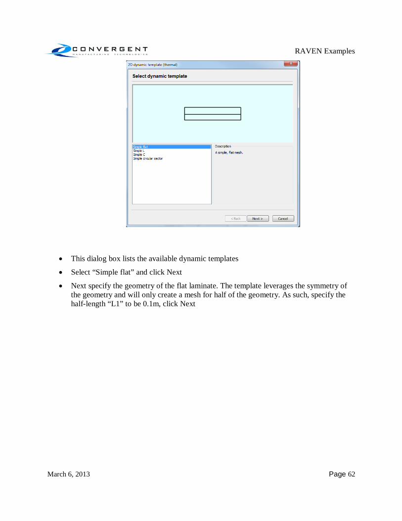
This dialog box lists the available dynamic templates

Select “Simple flat” and click Next

Next specify the geometry of the flat laminate. The template leverages the symmetry of the geometry and will only create a mesh for half of the geometry. As such, specify the half-length “L1” to be 0.1m, click Next

RAVEN Examples


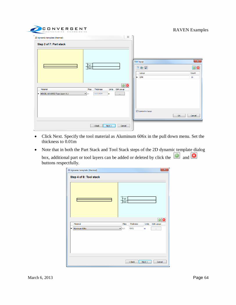
The part stack is defined next. Select the material HEXCEL AS4/8552 Tape from the drop down menu. Note that the thickness of the part is automatically calculated based on the number of plies and the ply thickness.

To adjust the number of plies, click the “…” button under the “Edit Layup” column heading.

The Edit Layup dialog box pops up.

Confirm that the layup is [0/90] symmetric and change the count to 16, click OK

RAVEN Examples


Click Next. Specify the tool material as Aluminum 606x in the pull down menu. Set the

thickness to 0.01m

Note that in both the Part Stack and Tool Stack steps of the 2D dynamic template dialog

box, additional part or tool layers can be added or deleted by click the and buttons respectfully.

RAVEN Examples


In the next step, select the MRCC average as the autoclave cycle. Click Next

Finally, define the boundary conditions all around the part. For the current 2D template, the envelope of the part is segmented in to the following regions:

Bag Side (BS) 60 W/(m2K)

Inside Tool (IS) 10 W/(m2K)

Left Side Part (LHSP) 50 W/(m2K)

Left Side Tool (LHST) 50 W/(m2K)

Right Side Part (RHSP) 50 W/(m2K)

Right Side Tool (RHST) 50 W/(m2K)

Change the Bag Side and Inside Tool heat transfer coefficients to 60 and 10 W/(m2K) respectively and click Next.

In the Post Processing step, accept the default plots to be generated.

Click Finish to run the analysis, it may take a few minutes

RAVEN Examples


By default, two plot tabs are created. The first shows the part thermal envelope. This is a plot of the maximum and minimum part temperature at any node in the model. The second tab shows the overall 2D temperature distribution at a given point in time. Use the slider under the Tools pane to move through the analysis time.

At a time of 160 min (which corresponds to the time of maximum exotherm, the thermal distribution should look like this:

RAVEN Examples


Example 8: Compare 2D and 1D thermal profile studies


Under the 2D tab in the Tasks pane, select “2D static template”

Raven will read the static templates stored on your local machine and open the 2D static

template dialog box

Select the template “Spar Section 30”

RAVEN Examples


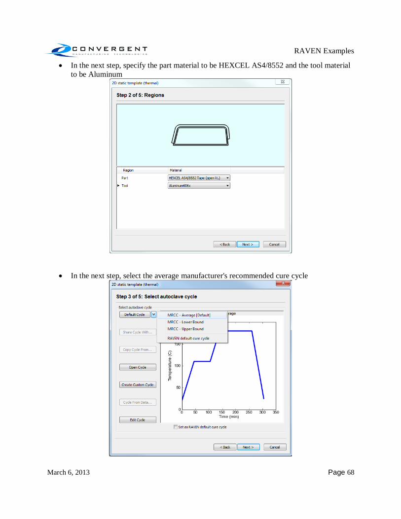
In the next step, specify the part material to be HEXCEL AS4/8552 and the tool material to be Aluminum

In the next step, select the average manufacturer's recommended cure cycle

RAVEN Examples


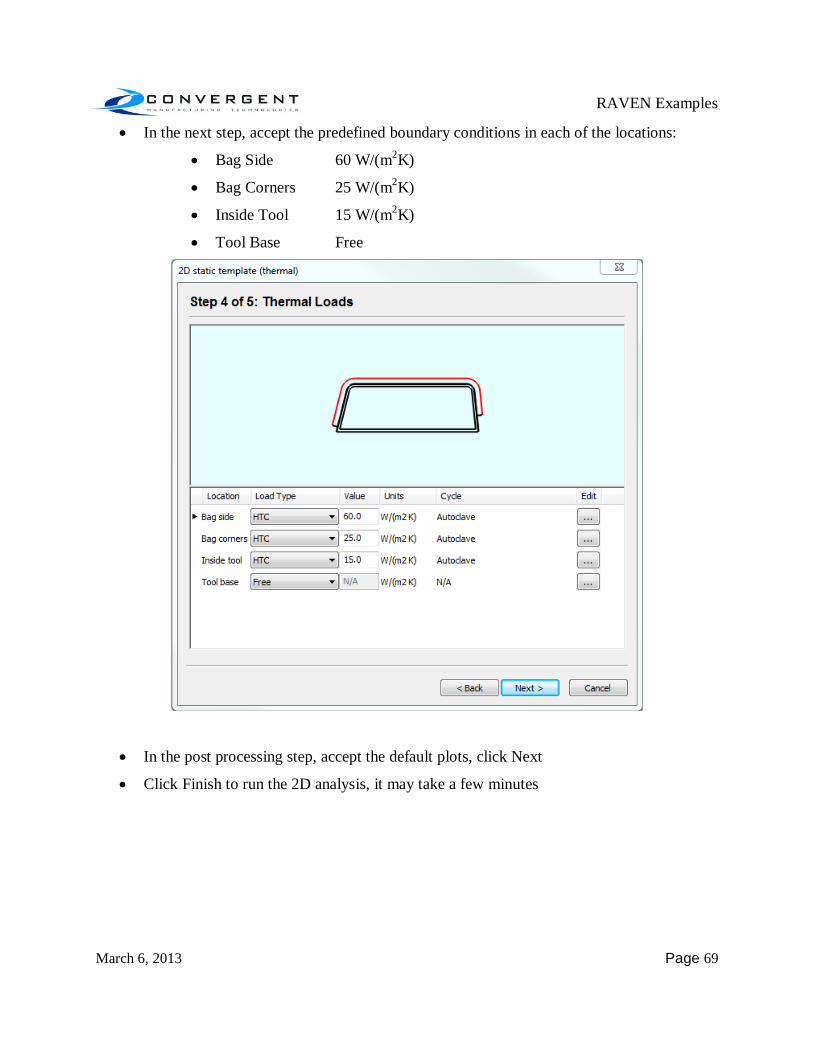
In the next step, accept the predefined boundary conditions in each of the locations:

Bag Side 60 W/(m2K)

Bag Corners 25 W/(m2K)

Inside Tool 15 W/(m2K)

Tool Base Free

In the post processing step, accept the default plots, click Next

Click Finish to run the 2D analysis, it may take a few minutes

RAVEN Examples


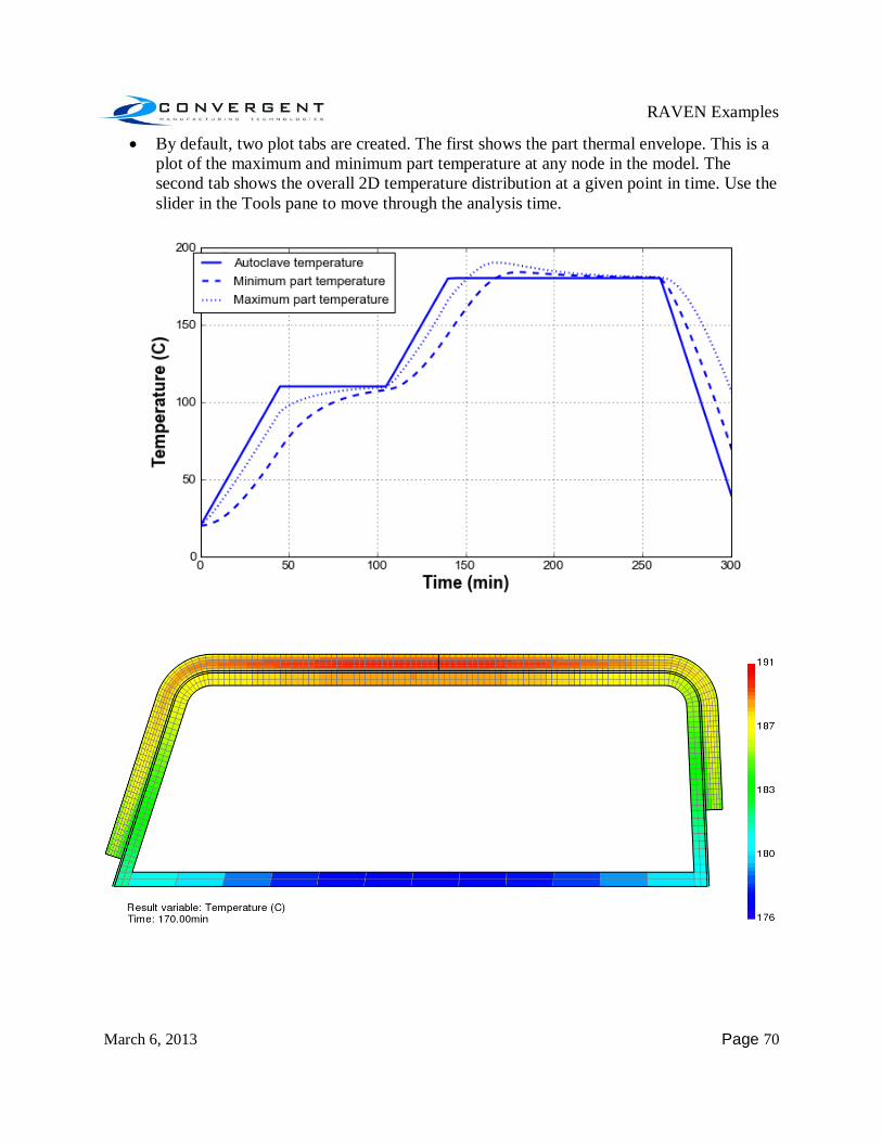
By default, two plot tabs are created. The first shows the part thermal envelope. This is a plot of the maximum and minimum part temperature at any node in the model. The second tab shows the overall 2D temperature distribution at a given point in time. Use the slider in the Tools pane to move through the analysis time.

RAVEN Examples


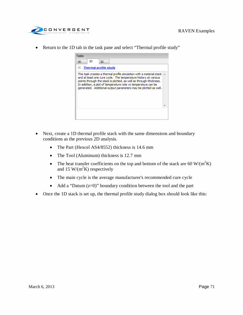
Return to the 1D tab in the task pane and select “Thermal profile study”

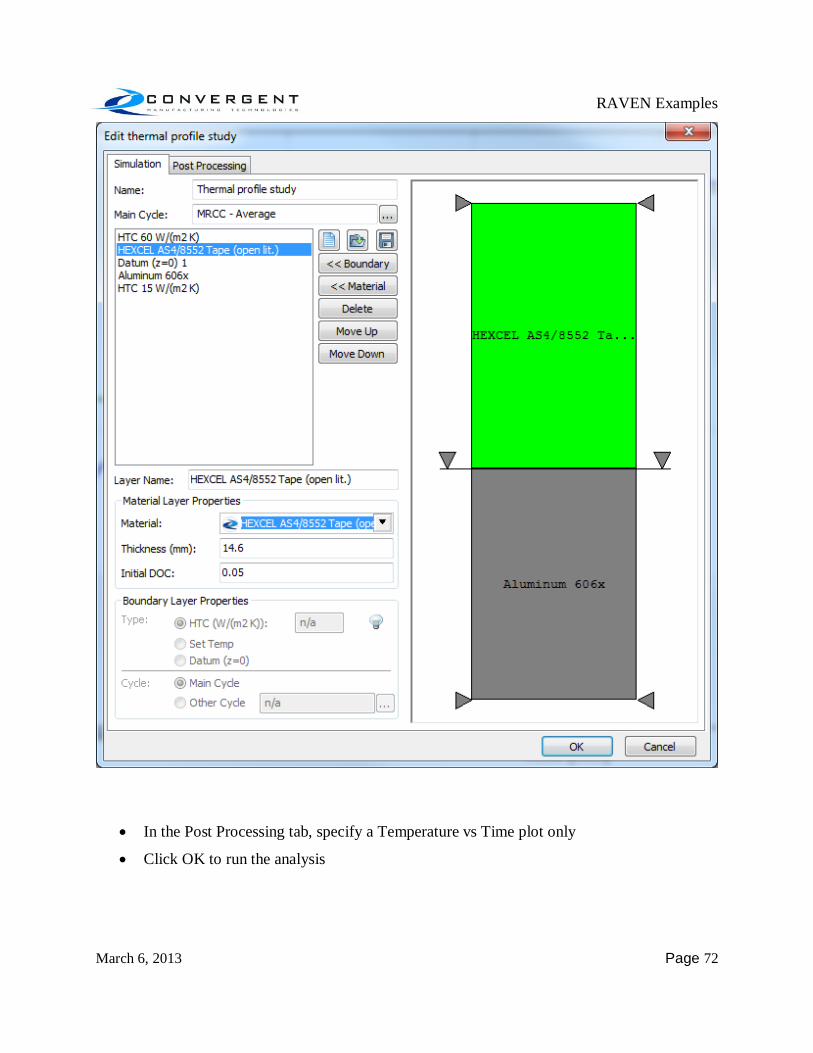
Next, create a 1D thermal profile stack with the same dimensions and boundary conditions as the previous 2D analysis.

The Part (Hexcel AS4/8552) thickness is 14.6 mm

The Tool (Aluminum) thickness is 12.7 mm

The heat transfer coefficients on the top and bottom of the stack are 60 W/(m2K) and 15 W/(m2K) respectively

The main cycle is the average manufacturer's recommended cure cycle

Add a “Datum (z=0)” boundary condition between the tool and the part

Once the 1D stack is set up, the thermal profile study dialog box should look like this:

RAVEN Examples


In the Post Processing tab, specify a Temperature vs Time plot only

Click OK to run the analysis

RAVEN Examples


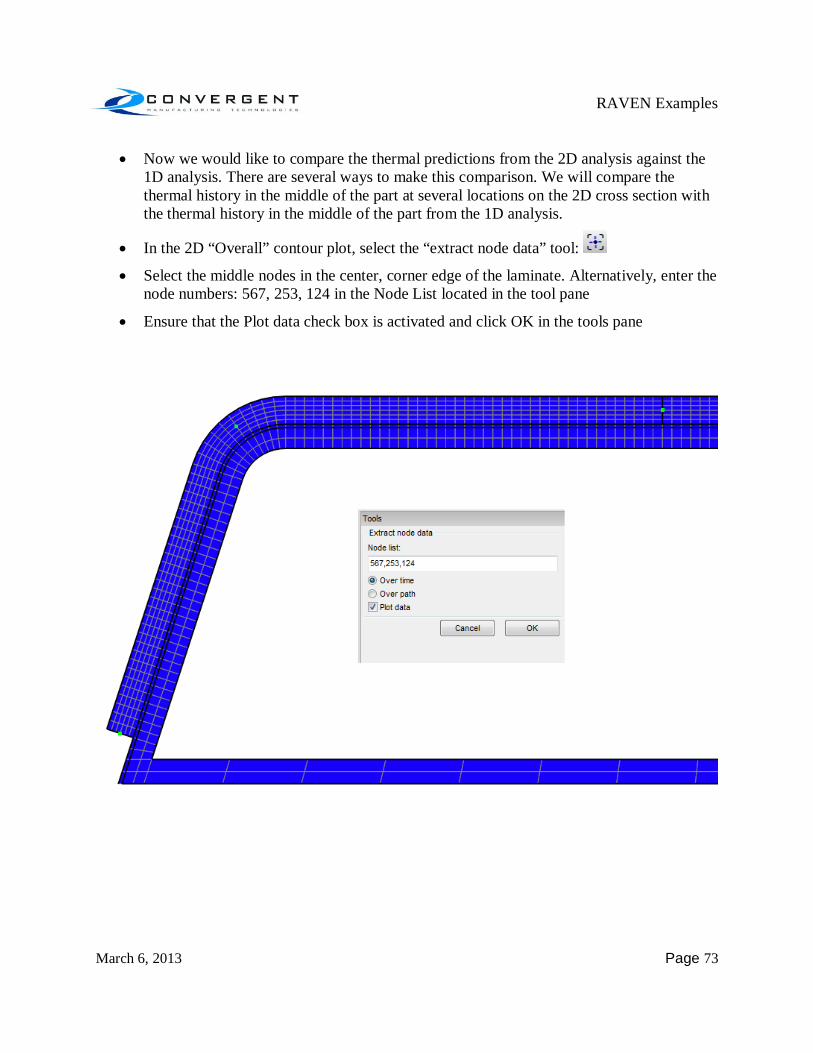
Now we would like to compare the thermal predictions from the 2D analysis against the 1D analysis. There are several ways to make this comparison. We will compare the thermal history in the middle of the part at several locations on the 2D cross section with the thermal history in the middle of the part from the 1D analysis.

In the 2D “Overall” contour plot, select the “extract node data” tool:

Select the middle nodes in the center, corner edge of the laminate. Alternatively, enter the node numbers: 567, 253, 124 in the Node List located in the tool pane

Ensure that the Plot data check box is activated and click OK in the tools pane

RAVEN Examples


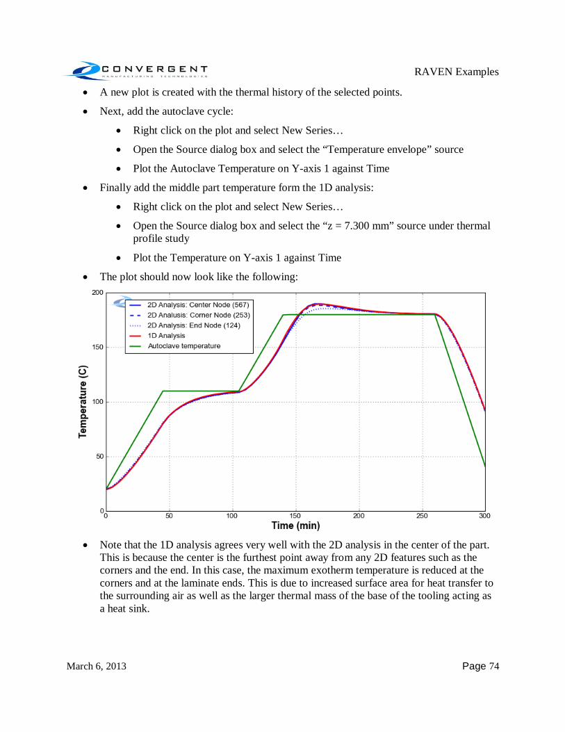
A new plot is created with the thermal history of the selected points.

Next, add the autoclave cycle:

Right click on the plot and select New Series…

Open the Source dialog box and select the “Temperature envelope” source

Plot the Autoclave Temperature on Y-axis 1 against Time

Finally add the middle part temperature form the 1D analysis:

Right click on the plot and select New Series…

Open the Source dialog box and select the “z = 7.300 mm” source under thermal profile study

Plot the Temperature on Y-axis 1 against Time

The plot should now look like the following:

Note that the 1D analysis agrees very well with the 2D analysis in the center of the part.

This is because the center is the furthest point away from any 2D features such as the corners and the end. In this case, the maximum exotherm temperature is reduced at the corners and at the laminate ends. This is due to increased surface area for heat transfer to the surrounding air as well as the larger thermal mass of the base of the tooling acting as a heat sink.

RAVEN Examples


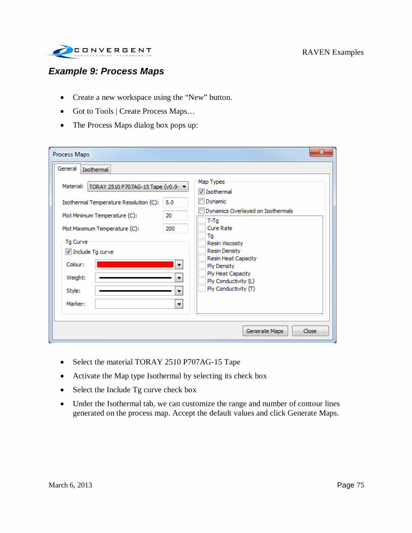
Example 9: Process Maps


Got to Tools | Create Process Maps…

The Process Maps dialog box pops up:

Select the material TORAY 2510 P707AG-15 Tape

Activate the Map type Isothermal by selecting its check box

Select the Include Tg curve check box

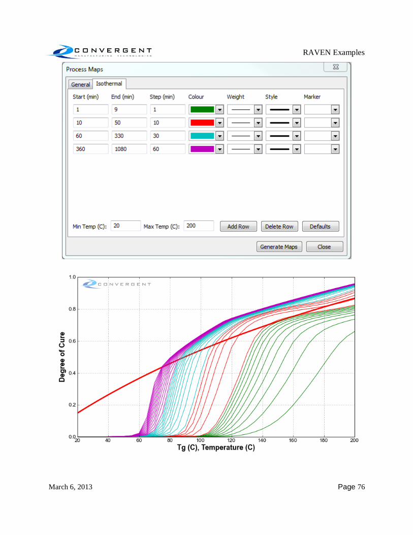
Under the Isothermal tab, we can customize the range and number of contour lines generated on the process map. Accept the default values and click Generate Maps.

RAVEN Examples


RAVEN Examples


The process map includes time contours in degree of cure versus temperature space.

Next we will plot the manufacturer's recommended fastest and slowest cure cycles on top of the process map to investigate how they differ.

Create a new Virtual Material Simulation by selecting the “sprocket” in the tool bar or click Data|New Simulation

In the Create new simulation dialog box, select the material TORAY 2510 P707AG-15

Tape

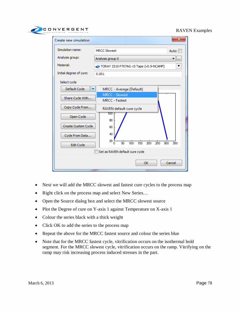
Name the simulation “MRCC Slowest”

Under the Default Cycle pull down menu, select the MRCC slowest cycle

Click Okay to run the analysis

Repeat the Virtual Material Simulation described above, however for this simulation, select the MRCC fastest cycle and name the simulation “MRCC fastest”

RAVEN Examples


Next we will add the MRCC slowest and fastest cure cycles to the process map

Right click on the process map and select New Series…

Open the Source dialog box and select the MRCC slowest source

Plot the Degree of cure on Y-axis 1 against Temperature on X-axis 1

Colour the series black with a thick weight

Click OK to add the series to the process map

Repeat the above for the MRCC fastest source and colour the series blue

Note that for the MRCC fastest cycle, vitrification occurs on the isothermal hold segment. For the MRCC slowest cycle, vitrification occurs on the ramp. Vitrifying on the ramp may risk increasing process induced stresses in the part.

RAVEN Examples


raven 3 examples - convergent · raven examples march 6, 2013 page 11 the resulting plot is shown...

Documents